Long-Term Profile Variability in Active Galactic Nuclei with Double-Peaked Balmer Emission Lines

Abstract

An increasing number of Active Galactic Nuclei (AGNs) exhibit broad, double-peaked Balmer emission lines,which represent some of the best evidence for the existence of relatively large-scale accretion disks in AGNs. A set of 20 double-peaked emitters have been monitored for nearly a decade in order to observe long-term variations in the profiles of the double-peaked Balmer lines. Variations generally occur on timescales of years, and are attributed to physical changes in the accretion disk. Here we characterize the variability of a subset of seven double-peaked emitters in a model independent way. We find that variability is caused primarily by the presence of one or more discrete “lumps” of excess emission; over a timescale of a year (and sometimes less) these lumps change in amplitude and shape, but the projected velocity of these lumps changes over much longer timescales (several years). We also find that all of the objects exhibit red peaks that are stronger than the blue peak at some epochs and/or blueshifts in the overall profile, contrary to the expectations for a simple, circular accretion disk model, thus emphasizing the need for asymmetries in the accretion disk. Comparisons with two simple models, an elliptical accretion disk and a circular disk with a spiral arm, are unable to reproduce all aspects of the observed variability, although both account for some of the observed behaviors. Three of the seven objects have robust estimates of the black hole masses. For these objects the observed variability timescale is consistent with the expected precession timescale for a spiral arm, but incompatible with that of an elliptical accretion disk. We suggest that with the simple modification of allowing the spiral arm to be fragmented, many of the observed variability patterns could be reproduced.

1 INTRODUCTION

It is now generally accepted that at the heart of an Active Galactic Nucleus (AGN) lies a supermassive black hole with a mass in excess of $10^{6}\;{\rm M_{\odot}}$ that is accreting matter from its host galaxy (see, e.g., Salpeter, 1964; Rees, 1984; Peterson, 1997). As matter spirals inward, it forms an equatorial accretion disk around the black hole (such as that described by Shakura & Sunyaev 1973), whose inner portions are heated to UV-emitting temperatures by “viscous” stresses which tap into the potential energy of the accreting gas.

The most direct kinematic evidence for large-scale accretion disks in AGNs comes from the broad, double-peaked Balmer emission lines detected in some AGNs. Double-peaked emission lines were first observed in the broad-line radio galaxies (BLRGs) Arp 102B (Stauffer, Schild, & Keel, 1983; Chen & Halpern, 1989; Chen, Halpern, & Filippenko, 1989), 3C 390.3 (Oke, 1987; Perez et al., 1988), and 3C 332 (Halpern, 1990). Given the similarity between these lines and those observed in cataclysmic variables (CVs), these authors suggested that the lines originated in an accretion disk surrounding the black hole at distances of hundreds to thousands of gravitational radii ($r_{g}$ = $G\;m_{\rm BH}/c^{2}$, where $m_{\rm BH}$ is the mass of the black hole). As discussed in great detail in Eracleous & Halpern (2003) and Gezari et al. (2007), alternative scenarios for the origin of the double-peaked lines are not consistent with the observed variability and multi-wavelength properties of double-peaked emitters. Thus we adopt this interpretation hereafter. A later survey of (mostly broad-lined) radio-loud AGN showed that $\sim$ 20% of the observed objects exhibited double-peaked Balmer emission lines (Eracleous & Halpern, 1994, 2003). Strateva et al. (2003) found 116 double-peaked emitters in the Sloan Digital Sky Survey (SDSS; York, 2000), representing 3% of the $z<0.332$ AGN population. In addition, several Low Ionization Nuclear Emission-line Regions (LINERs, Heckman, 1980) were found to have double-peaked Balmer lines, including NGC 1097 (Storchi-Bergmann, Baldwin, & Wilson, 1993), M81 (Bower et al., 1996), NGC 4203 (Shields et al., 2000), NGC 4450 (Ho et al., 2000), and NGC 4579 (Barth et al., 2001). Most recently, Moran et al. (2007) discovered that the obscured AGN NGC 2110 shows a double-peaked H$\alpha$ emission line in polarized light.

The prototypical double-peaked emitters (Arp 102B, 3C 390.3, and 3C 332) exhibited variations in their line profiles that took place on timescales of years (for examples, see Veilleux & Zheng, 1991; Zheng, Veilleux, & Grandi, 1991; Gilbert et al., 1999; Shapovalova et al., 2001; Sergeev, Pronik, & Sergeeva, 2000, 2002; Gezari, Halpern, & Eracleous, 2007), with the most striking variability being occasional reversals in the relative strength of the red and blue peaks. This long-term variability is intriguing because it is un-related to more rapid changes in luminosity but might be related to physical changes in the accretion disk. This profile variability can be exploited to test various models for physical phenomena in the outer accretion disk.

The observed long-term variability of the double-peaked line profiles (on time scales of several months to a few years) and the fact that in many objects the red peak is occasionally stronger than the blue peak (in contrast to the expectations from relativistic Doppler boosting) mandates that the accretion disk is non-axisymmetric. A few of the best-monitored objects (Arp 102B, 3C 390.3, 3C 332, and NGC 1097) have been studied in detail using models that are simple extensions to a circular accretion disk. These include circular disks with orbiting bright spots or “patches” (Arp 102B and 3C 390.3, Newman et al., 1997; Sergeev, Pronik, & Sergeeva, 2000; Zheng, Veilleux, & Grandi, 1991), a disk which is composed of randomly distributed clouds that rotate in the same plane (Arp 102B, Sergeev et al., 2000), spiral emissivity perturbations (3C 390.3, 3C 332, and NGC 1097, Gilbert et al., 1999; Storchi-Bergmann et al., 2003) and precessing elliptical disks (NGC 1097, Eracleous et al., 1995; Storchi-Bergmann et al., 1995, 1997, 2003). All of these non-axisymmetric models naturally lead to modulations in the ratio of the red to blue peak flux; in the case of the first two models, modulations occur on the dynamical timescale whereas for the latter two, the variations occur on the longer precession timescale of the spiral density wave or the elliptical disk. However, in all cases, these simple models do not reproduce the fine details of the profile variability.

It is extremely important to determine whether the profile variability observed in the small number of well-monitored objects is common to all double-peaked emitters. With a larger sample, one can determine if there are universal variability patterns that point to a global phenomenon that occurs in AGN accretion disks. Thus, a campaign was undertaken to observe a larger sample of $\sim$20 radio-loud double-peaked emitters from the Eracleous & Halpern (1994) sample, in addition to a few more recently discovered objects. This campaign spanned nearly a decade and many objects were observed 2–3 times per year, although some objects, particularly those in the southern hemisphere, were only observed once per year. In this paper we present results for seven objects whose long-term variability has not been studied in any detail: 3C 59, 1E 0450.3–1817, Pictor A, CBS 74, PKS 0921–213, PKS 1020–103, and PKS 1739+18C. The properties of these objects are given in Table 1 and a plot of the temporal coverage of the observing campaign is provided in Figure 1. Gezari et al. (2007) present results for Arp 102B, 3C 390.3, 3C 332, PKS 0235+023, Mkn 668, 3C 227, and 3C 382. The most recent profile variability results for NGC 1097 are presented by Storchi-Bergmann et al. (2003), while the remaining objects from this monitoring program will be presented in Flohic et al. (2010, in preparation).

The primary goal of this paper is to characterize the observed variability patterns in these seven objects in a model-independent way. Currently, the models which have been used to fit the line profiles represent the most simple extensions to a circular disk. As mentioned above, these models fail to reproduce the fine details of the profile variability. A detailed characterization of the variability will help guide the refinement of these models and more importantly inspire ideas for new families of models. In essence, these results will serve as benchmark that models can be easily tested against.

This paper is organized as follows. In §2, the observations and data reductions are described. §3 is devoted to describing the methods for characterizing the profile variability in a model-independent way and noting the common trends in the data. In §4 we detail the two simple models we will compare with the observations, including their physical motivation, the model profile calculation, and the common variability trends. In §5 we assess the viability of these two models through a comparison of the observed and predicted variability trends and timescales. We also suggest refinements to the models which might afford a better description of the observed variability trends. Finally, in §6 we summarize the primary findings.

2 OBSERVATIONS AND DATA REDUCTIONS

The majority of the spectra were obtained over the period from 1991–2004 using the 2.1m and 4m telescopes at Kitt Peak National Observatory (KPNO), the 1.5m and 4m telescopes at Cerro-Tololo Inter-American Observatory (CTIO), the 3m Shane Telescope at Lick Observatory, the 1.3m and 2.4m telescopes at the MDM Observatory, and the 9.2m Hobby-Eberly Telescope (HET) at the McDonald Observatory. A complete list of the spectrographs and gratings used is provided in Table 2 and a journal of the observations is given in Table 3. The spectra were taken through a narrow slit (1.$\!\!{}^{\prime\prime}$25 – 2.$\!\!{}^{\prime\prime}$0) and the seeing varied from 1$\arcsec$–3$\arcsec$. The spectra were extracted from a 4$\arcsec$-8$\arcsec$ wide region along the slit and the resulting spectral resolution ranged from 3$\arcsec$–8$\arcsec$; the resolution for each instrumental configuration is listed in Table 2. Most of the data reductions were carried out by us, although some spectra were provided in reduced form by A. V. Filippenko (see also the notes to Table 3.) The primary data reductions—the bias level correction, flat fielding, sky subtraction, removal of bad columns and cosmic rays, extraction of the spectra, and wavelength calibration—were performed with the Image Reduction and Analysis Facility (IRAF). Flux calibration was performed using spectrophotometric standard stars drawn from Oke & Gunn (1983), Stone & Baldwin (1983) or Baldwin & Stone (1984) that were observed at the beginning and end of each night. Although the relative flux scale is accurate to better than 5%, the absolute flux scale is uncertain by up a factor of 2 due to the small slit used and the occasional non-photometric sky conditions. There are several atmospheric features that contaminate the spectra, namely the ${\rm O_{2}}$ bands near 6890Å  and 7600Å  (the B- and A- bands, respectively) and the water-vapor bands near 7200Å  and 8200Å. These were corrected using templates constructed from the (featureless) spectra of the standard stars.

3 PROFILE ANALYSIS

Before analyzing the spectra, they were shifted into the rest frame of the source and corrected for Galactic reddening, using the redshifts and color excesses given in Table 1. Then the underlying continuum (from both stellar and non-stellar sources) was modeled, using the combination of a spectrum of an inactive elliptical galaxy and a powerlaw continuum, and subtracted. There was often residual curvature in the continuum around the broad H$\alpha$ profile that was removed using a low (1^st or 2^nd) order polynomial. These processes of continuum subtraction, particularly that of the local continuum, introduce some uncertainty which will be discussed and quantified below as necessary. In addition, small wavelength shifts were applied based on the measured wavelength of the narrow H$\alpha$ emission line and the spectra were re-sampled to have a uniform wavelength scale. The profiles after continuum subtraction are displayed in Figures 2–8. The spectra have been scaled such that the narrow emission line fluxes are identical in each observation, as described in §3.1. These profiles, and their variations with time, will be characterized in the following sections.

3.1 Measurement of Narrow and Broad-Line Fluxes

We use the narrow emission lines to provide a relative flux calibration between spectra, since these lines are thought to originate in a very extended region around the AGN and they are not expected to respond to rapid variations in continuum flux (see, e.g., Peterson, 1993). The narrow emission lines covered by these spectra include [O i]$\lambda\lambda$6300,6363, [N ii]$\lambda\lambda$6548,6583, [S ii]$\lambda\lambda$6716,6730, and the narrow component of H$\alpha$.

The narrow emission lines of interest lie on top of the broad double-peaked H$\alpha$ line, which must be removed prior to measuring the flux of the narrow lines. The [O i]$\lambda$6300,[O i]$\lambda$6363 and [S ii]$\lambda\lambda$6716,6730 lines lie on the wings of the double-peaked ${\rm H\alpha}$ emission line. Repeated subtraction of the underlying broad wings, fitted with a 3^rd order polynomial, indicates that the flux of the [O i]$\lambda$6300 and the [S ii]$\lambda\lambda$6716,6730 can be measured robustly (with $\lesssim$ 10% variation). The weak [O i]$\lambda$6363 has a larger uncertainty (20%).

The [N ii] and narrow H$\alpha$ emission lines are often blended, at least at the base. The blend is decomposed by first fitting the [N ii]$\lambda$6583 and [N ii]$\lambda$6548 emission lines in a 3:1 flux ratio and then fitting the residual narrow H$\alpha$ line. For any given fit to the underlying broad-line, the line fluxes of the [N ii] and narrow H$\alpha$ line can be measured with an accuracy similar to the other narrow emission lines ($\sim$ 10%–15%). However, the process of subtracting the underlying broad-line is more ambiguous because these lines lie on the trough of the double-peaked profile. We found that the process of removing the underlying broad component can introduce a systematic uncertainty of up to 30%.

It is possible to guard against the systematic uncertainty by considering the ratios of the narrow line fluxes (i.e. [O i]/[S ii], [S ii]/H$\alpha$, [O i]/H$\alpha$, and [N ii]/H$\alpha$) which should not change significantly with time. It is still possible that the H$\alpha$+[N ii] flux are systematically uncertain, but no significant variations in the narrow line fluxes will be introduced, because all spectra are affected in the same manner.

To determine the broad-line flux (${\rm F_{broad\;H\alpha}}$) the total narrow line flux determined above was simply subtracted from flux of the entire profile (narrow + broad). The estimated errors on the total flux and narrow line flux were added in quadrature to obtain an approximate error in the broad-line flux. The narrow lines in PKS 1739+18C, with the exception of [O i]$\lambda 6300$, could not be measured because the profile is dominated by the broad double-peaked component. Because the narrow lines probably contribute only 5–10% of the total flux in this object, we simply used the total measured flux in lieu of the broad-line flux. We also consider absolute changes in the broad-line flux by normalizing each broad-line flux by the [O i]$\lambda 6300$ line flux. The reported error on the normalized broad-line flux include those from both the broad-line and [O i]$\lambda 6300$ fluxes.

In the next three sub-sections, we present three different methods for characterizing the variations in double-peaked line profiles in a model-independent way. After the results for each method are presented, we first describe general trends and then highlight results from specific objects.

3.2 RMS and Correlation Plots

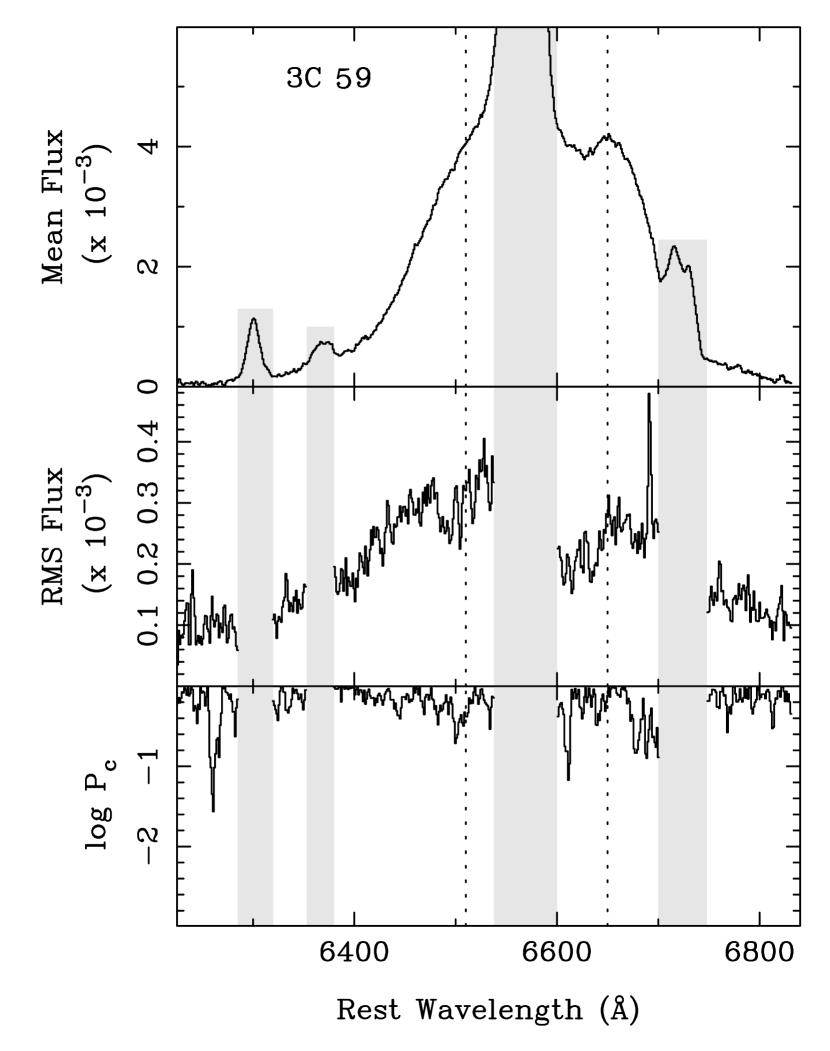
Figure 9: Top: the mean profile of 3C 59, constructed from profiles normalized by their total broad H$\alpha$ flux. Middle: the rms variability, as a function of wavelength. Bottom: the log of the chance probability that there is a spurious correlation between the total broad-line flux and the broad-line normalized profile flux, determined with a Spearman’s rank-order correlation test. A small chance probability indicates that there may be a correlation. The vertical dashed lines indicate the position of the peaks in the mean profile and the vertical gray stripes indicate the positions of the narrow emission lines, which were not removed. See §3.2 for more details.

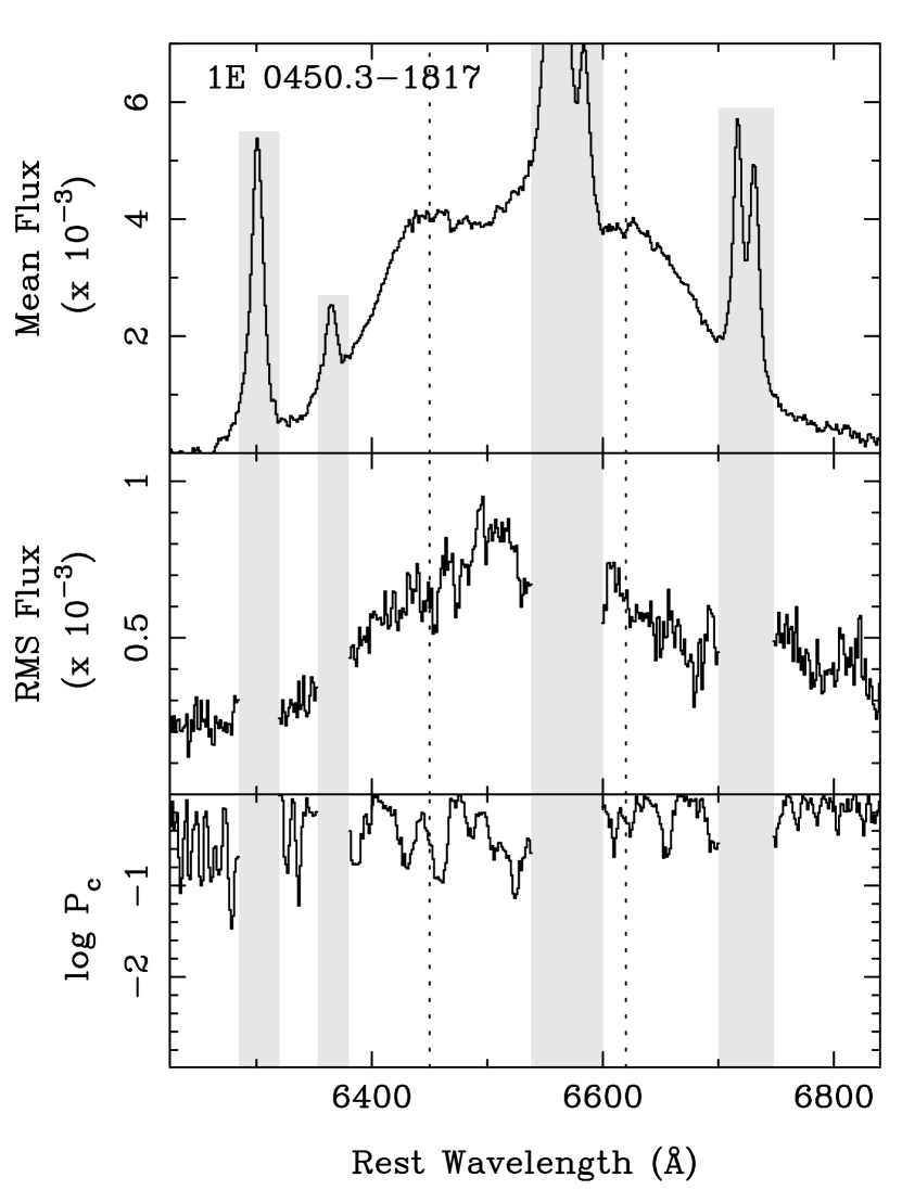
Figure 10: Same as Figure 9, but for 1E 0450.3–1817.

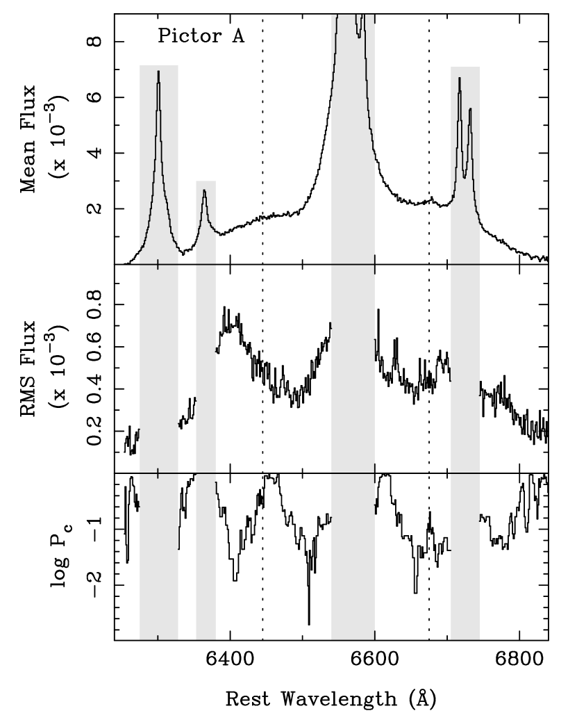
Figure 11: Same as Figure 9, but for Pictor A.

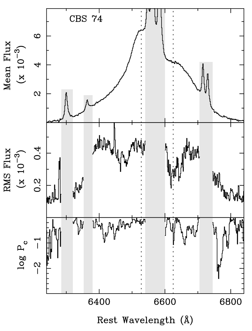
Figure 12: Same as Figure 9, but for CBS 74.

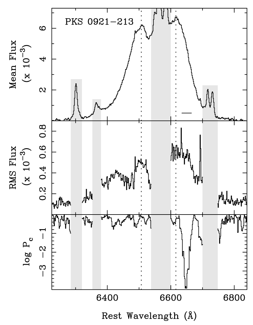
Figure 13: Same as Figure 9, but for PKS 0921–213. The plot of the chance probability indicates that there may be a correlation between the broad-line normalized flux integrated over the 6635–6665Å wavelength interval (indicated by the horizontal bar in the top panel) and ${\rm F_{broad\;H\alpha}}/{\rm F_{[O\;I]}}$ is explored further in Figure 14.

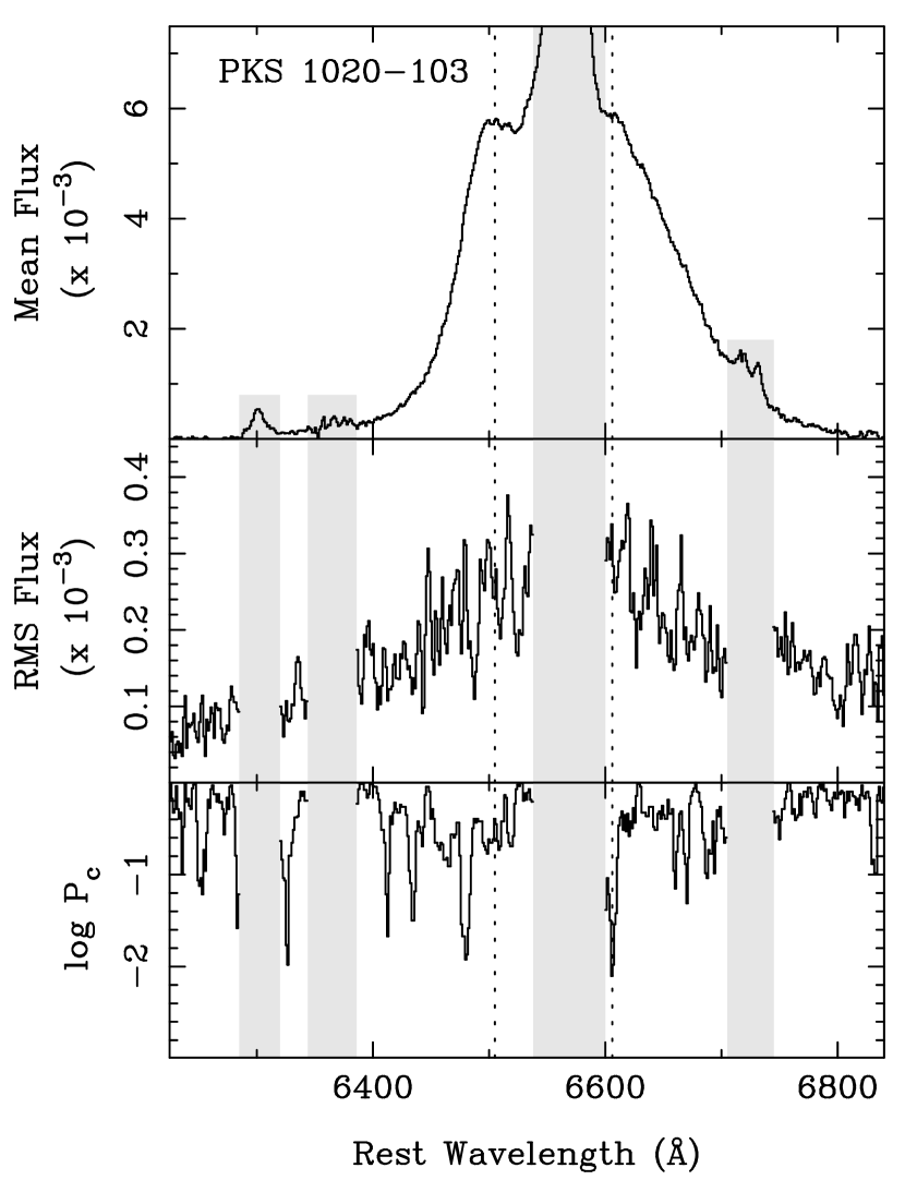
Figure 15: Same as Figure 9, but for PKS 1020–103.

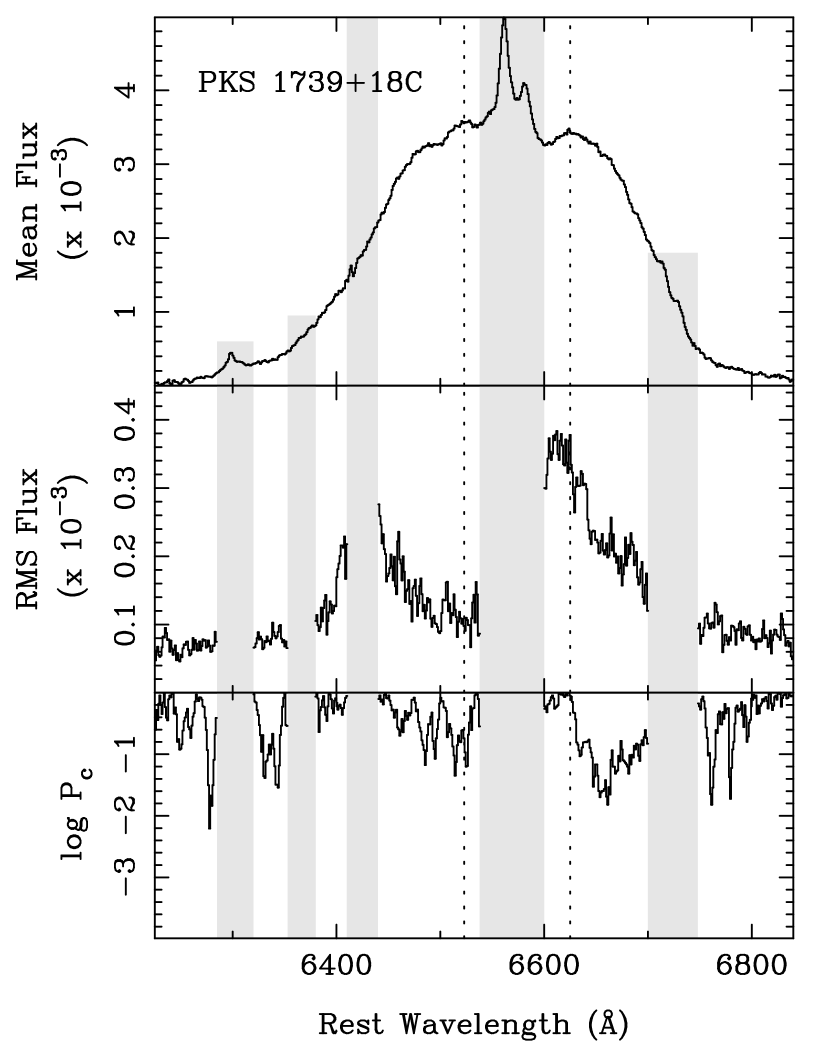
Figure 16: Same as Figure 9, but for PKS 1739+18C. An additional gray stripe indicates the region of the spectrum affected by telluric A-band ($\sim$7400–7440$\AA$ at the redshift of this object.) Imperfect removal of the telluric features may result in spurious rms variability. Imperfect removal of the telluric features may result in spurious features in the difference spectra.

As shown in Figures 2–8, the broad H$\alpha$ profiles clearly change with time. We first investigate whether some portions of the profile are more variable than others by plotting the root mean square (rms) flux variations as a function of wavelength. Short-term fluctuations in the illumination will cause the total broad-line flux to change (i.e. through light reverberation), as observed in 3C 390.3 (Dietrich, 1998; Shapovalova et al., 2001). Because we are primarily concerned with changes in the shape of the profile rather than changes in the overall flux, the spectra were normalized by the broad line flux (i.e.we convert $f_{\lambda}$ to $f_{\lambda}\;\Delta\lambda/{\rm F_{broad\;H\alpha}}$, where $\Delta\lambda$ is the resolution element) before constructing the mean and rms profiles. In Figures 9–16, we show the mean profile in the top panel, and the rms profile in the middle panel.

The rms profile for most objects is quite different from the mean profile, indicating that the profile is not uniformly variable. Many objects do show considerable variability at wavelengths that roughly coincide with a peak in the mean profile (e.g. both peaks of 3C 59, PKS 0921–213, and the red peaks of Pictor A and PKS 1739+18C, and the blue peak of CBS 74). In some objects however, there are minima in the rms profiles at locations of the peaks (the red peak of CBS 74 and the blue peak of PKS 1739+18C) indicating that the flux of these peak regions are unusually stable compared with the rest of the profile.

For some objects, there are distinct features in the rms profile that are at significantly larger projected velocity than the peaks in the mean profile (e.g. 3C 59, Pictor A, CBS 74, PKS 0921–213, PKS 1739+18C). Increased variability at large projected velocity is consistent with the idea that the inner portions of the line-emitting disk (which give rise to the wings of the profile) could vary on a shorter timescale than the outer regions of the disk. For 1E 0450.3–1817 and PKS 1020–103, the rms profiles do not show many distinct features. We do note that 1E 1E 0450.3–1817 is slightly more variable at negative projected velocities, with a maximum at $\sim 6500$ Å (see Figure 10).

One could also expect to find a narrower, single-peaked variable component in the middle of the profile between the two peaks. However, because the narrow H$\alpha$+[N ii] lines were not subtracted, it is difficult to detect a single-peaked component unless it has ${\rm FWHM}\gtrsim 2000\;{\rm km\;s^{-1}}$ or the line is significantly blue- or redshifted with respect to the narrow H$\alpha$ line. In Pictor A there is a central peak in the rms variability profile that is slightly blue-shifted with respect to narrow H$\alpha$; this is most likely due to the single-peaked, broad H$\alpha$ component (${\rm FWHM}\sim 3000\;{\rm km\;s^{-1}}$) which is very obvious in this object. Three other objects (3C 59, CBS 74, and 1E 0450.3–1817) show features in the central regions of the rms profile ($\lambda\sim 6500-6530{\rm\AA}$).In all three objects, there is a blue peak or shoulder at a similar wavelength. If related to a single-peaked H$\alpha$ line, the line would be blue-shifted by $\sim 1000-3000{\rm km\;s^{-1}}$ relative to the narrow H$\alpha$ line; although such blue-shifts are observed in high-ionization lines (such as C IV), they are not common in the low-ionization Balmer lines (Sulentic et al., 2000). Thus these features are more likely to be associated with the blue peak or shoulder seen in the mean profile, rather than a single-peaked broad H$\alpha$ component.

We note that Gezari et al. (2007) also find that structure in the rms profile often occurs at larger projected velocity than the peaks in the mean profile. These authors were able to perform narrow-line subtraction and, as a result, were able to detect central peaks in the rms profiles of Arp 102B and 3C 332 with velocity widths of $\sim 1000\;{\rm km\;s^{-1}}$. This suggests that a “standard” single-peaked component may be present in those objects.

It is possible that the double-peaked line profile might vary in response to long-term, secular variations in the illuminating flux which could alter the physical properties of the disk (such as the ionization state). Such long-term effects have been noticed in NGC 1097 (Storchi-Bergmann et al., 2003) and 3C 332 (Gezari et al., 2007). To investigate whether the profile varies in response to long-term changes in the broad-line flux, we looked for correlations between ${\rm F_{broad\;H\alpha}}/{\rm F_{[O\;I]}}$ and the flux in the normalized line profile ($f_{\lambda}\;\Delta\lambda/{\rm F_{broad\;H\alpha}}$) integrated over five-pixel bins centered on $\lambda$. We used the non-parametric Spearman’s rank-order correlation test (see, e.g. Press et al., 1992), since we do not know what functional form any potential correlation will take. In the bottom panel of Figures 9–16, the log of the chance probability ($P_{c}$) is plotted as a function of wavelength, where $P_{c}$ is the chance probability that the correlation is spurious.

We plotted the broad H$\alpha$ flux (relative to [O i]) versus the integrated normalized profile flux for any region in which $P_{c}<0.1$, but in most instances there was either little obvious correlation or the correlation was driven by a few data points. A wavelength interval redward of the red peak ($\lambda$=6635–6665${\rm\AA}$ in PKS 0921-0213 does show a possible negative correlation (see Figure 14). It must be noted that the broad-line flux in PKS 0921–213 decreases nearly monotonically; thus it is impossible to ascertain whether the flux in this wavelength interval is decreasing in response to a decrease in the total broad H$\alpha$ flux (and presumably the illuminating flux) or some other, perhaps dynamical, effect which is also steadily varying with time. We come back the issue of long-term correlations between the broad-line profile and the illuminating flux in §3.4.

3.3 Difference Spectra

In order to better visualize the profile variability, we present here difference spectra that result from subtracting either the mean or the “minimum” profile. The latter is constructed by selecting, at each wavelength, the minimum flux density from among all the spectra of the same object. This minimum spectrum represents a base profile which is common to all the profiles. As an idealized example, if the emission arises from a circular accretion disk with an emissivity enhancement (such as a hot spot or spiral arm), then the minimum profile would be that of the underlying circular accretion disk. The difference spectra from the minimum would clearly reveal the (positive) emissivity enhancement as it travels through the disk and affects different portions of the emission line profile. However, even in this idealized scenario, one must use caution in interpreting the minimum profile. In the simple additive models mentioned above, the variability is expected to be cyclical. The minimum profile will not be equivalent to the profile of the underlying disk if only a portion of the cycle has been observed (see §5.1).

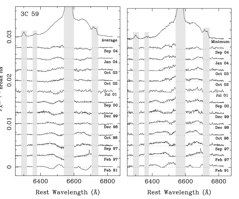
Figure 17: Difference spectra for 3C 59. In the left panel, the average spectrum and the difference between each spectrum and the average are shown, whereas the minimum and the differences from it are shown in the right panel. Arbitrary vertical offsets were applied for clarity. The vertical gray stripes indicate the positions of the narrow emission lines. See §3.3 for a description of how these spectra were constructed.

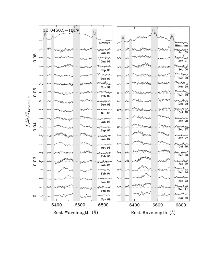
Figure 18: Same as Figure 17, but for 1E 0450.3–1817.

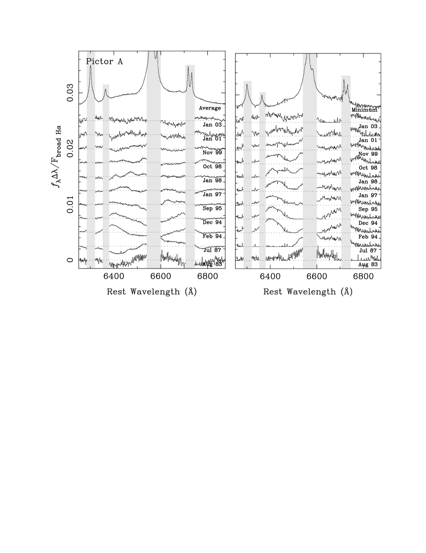
Figure 19: Same as Figure 17, but for Pictor A.

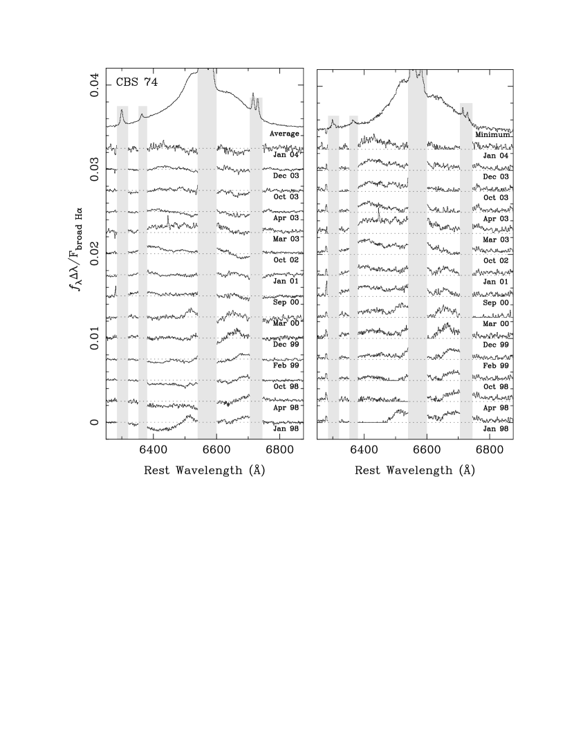
Figure 20: Same as Figure 17, but for CBS 74.

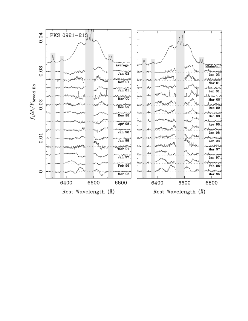
Figure 21: Same as Figure 17, but for PKS 0921–213.

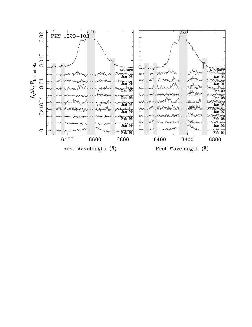
Figure 22: Same as Figure 17, but for PKS 1020–103.

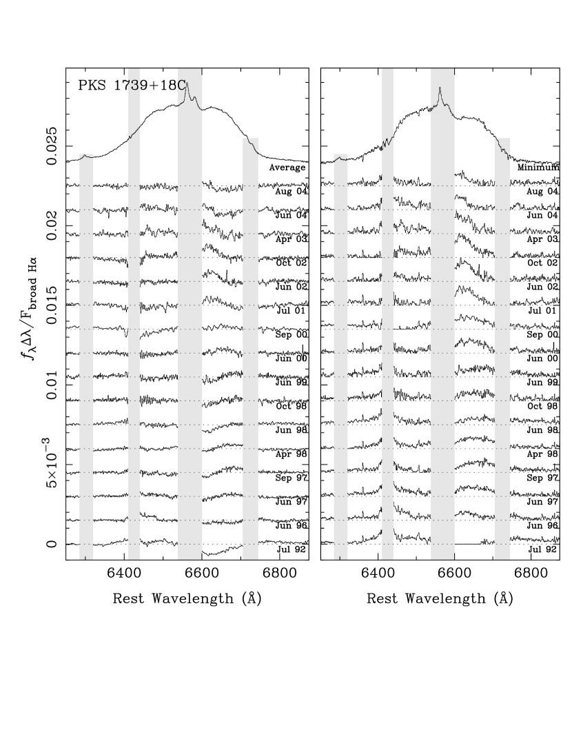
Figure 23: Same as Figure 17, but for PKS 1739+18C. An additional gray stripe indicates the region of the spectrum affected by telluric A-band ($\sim$7400–7440$\AA$ at the redshift of this object.)

The mean and minimum comparison spectra were subtracted from each individual spectrum and the resulting difference spectra are shown in Figures 17–23. As with the rms profiles, we are not concerned with the variations in the broad-line flux, thus the profiles were normalized as described above. Because the spectra were renormalized by their broad-line flux, the narrow emission lines will vary from one observation to the next. Rather than remove the narrow lines, which would require assumptions about the shape of the underlying profile, these regions were simply not plotted in the difference spectra and the omitted regions are indicated by vertical gray stripes. As can be seen in Figures 17–23, the prominent features in the difference spectra are generally broader than the omitted spectral regions, thus these gaps do not greatly impair the interpretation of the difference spectra.

There are several trends commonly seen in the difference spectra of most objects. In general, trends are best illustrated by the differences from the minimum spectrum.

1. The difference spectra suggest the presence of distinct “lumps” of emission, and typically there are multiple lumps, sometimes at both negative and positive projected velocities, at any given time. The amplitude of these lumps, relative to the flux in the minimum spectrum at the position of the lump, is typically 20–30% although when the lump is located at the wings of the profile, the relative flux is much larger ($\sim$ 50%). The lumps typically represent 5–10% of the total broad H$\alpha$ flux. An exception is Pictor A, in which the spectrum has undergone significant changes in profile shape; the flux in the “lumps” of emission is several times larger than in either the minimum or the average spectrum, and the lumps are as much as 20% of the total broad-line flux. The changes in these distinct “lumps” of excess emission, either in shape, amplitude, or projected velocity, are primarily responsible for the variability in the line profiles.

2. Neither the average nor, more importantly, the minimum spectra are consistent with the expected profile from a circular accretion disk, because the red peak is often as strong as, or stronger than, the blue peak. This may be due to the fact that if only a partial variability cycle has been observed, the minimum profile will not be that of the underlying disk; we explore this further in §5.1. However, another possibility is that if the profile variability can indeed be explained as an underlying disk with extra, transient lumps of emission, the underlying disk itself may not be axisymmetric and thus the “base” (i.e. minimum) profile would vary on long timescales (e.g. if the underlying disk is elliptical, then the base profile will precess as described in §5.2). One should be cautious in associating the minimum spectrum with the profile of an underlying “static” disk to which all other features are added.

3. The less luminous systems (1E 0450.3–1817, Pictor A, and PKS 0921–213) vary on shorter timescales than the more luminous systems. The black hole masses ($M_{BH}\sim 4\times 10^{7}{\rm M_{\odot}}$) for these three objects have been estimated from the stellar velocity dispersion (Lewis & Eracleous, 2006), and the physical timescales for the variability in these objects will be discussed in more detail in §5.

4. If one assumes that lumps from one observation epoch can be tracked in following observations, several general conclusions can be drawn.

   1. The lumps can persist for several years; in a few objects, some lumps appear to persist throughout the duration of the monitoring observations such as the red lumps in 3C 59 and PKS 1739+18C. These lumps still do vary slightly in amplitude and shape, but they do not dissipate completely.

   2. When the lumps do disappear over time, they typically arise on rather short timescales ($\lesssim$ one year) and dissipate more slowly (over several years), generally becoming broader in the process of decaying.

   3. Lumps can drift across the profile in either direction. We note that it is more common for lumps to drift from positive to negative, reminiscent of Arp 102B (Sergeev et al., 2000). However Gezari et al. (2007) do not observe such a trend in the longer-baseline observations of Arp 102B, nor in any of the other objects in their sample.

1E 0450.3–1817, Pictor A, CBS 74 and PKS 0921–213 all show striking variability which we describe in more detail here.

1E 0450.3–1817. – This object is unique in the large number of distinct lumps which have appeared, drifted across the profile, and dissipated; during some observation epochs there are up to three different lumps present at once. The lumps emerged at both small and large (as well as negative and positive) projected velocities. Some of the lumps are long-lived and do not vary significantly in strength, shape, or position over a period of $\sim$ 8 years, whereas other lumps emerge, drift, and dissipate over four years.

Pictor A. – This object shows the most dramatic variability, in the sense that the line was not observed to be double-peaked prior to 1994 (Halpern & Eracleous, 1994; Sulentic et al., 1995). The blue lump originated at a projected velocity of $v_{p}\sim 7500\;{\rm km\;s^{-1}}$, suggesting that the emitting gas is located at characteristic radius ($r_{c}$) of less than $1500\;r_{g}\;\sin^{2}i$, where $i$ is the angle between the line of sight and the axis of the disk. Eracleous & Halpern (2003) find that $i\sim 30{\rm{}^{\circ}}$ when an elliptical disk model is used, and $i>65^{\rm{\circ}}$ for a circular disk. This lump steadily drifted to less negative projected velocity ($\Delta v_{p}\sim 3000\;{\rm km\;s^{-1}}$) over a period of approximately 4 years and has been dissipating slowly throughout the campaign. The red lump originated at an earlier time and also drifted towards smaller projected velocity, however it significantly decreased in intensity over the first several years.

CBS 74. – The blue side of the profile as a whole is quite variable after 1998 October, and it is difficult to describe in terms of individual lumps of emission. A lump on the red side of the profile steadily increased strength and then began to decrease again over a 5 year period. This lump of emission drifted blueward at first and then drifted slightly redward before dissipating.

PKS 0921–213. – The profile of this object in the early observations is very unusual and appears to have two double-peaked components, one with closely separated peaks overlying another with more widely separated shoulders. Within a year, the closely-spaced component appears to dimish, leaving a double-peaked profile that has peaks with an intermediate spacing. After this, the most prominent feature is a red lump, at a projected velocity of $\sim 4500\;{\rm km\;s^{-1}}$, suggesting a characteristic radius of less than $4000\;r_{g}\;\sin^{2}i$ ($i>40^{\circ}$; Eracleous & Halpern, 2003) that strengthened over two years then drifted towards lower projected velocity by $\sim 2000\;{\rm km\;s^{-1}}$ and was still quite strong during the last observation.

In the above descriptions, we have assumed that one can track a lump from one epoch in subsequent observations. This does not necessarily imply that the same parcel of gas is responsible for the emissivity enhancement. Indeed this cannot be the case, at least for PKS 0921–213 and 1E 0450.3–1817, if these gas parcels are part of a Keplerian disk. The dynamical timescales for these objects are known to be only a few months (Lewis & Eracleous, 2006) and each of these objects was closely monitored at times (with gaps of only 1–2 months between observations); there was clearly no orbital motion. Thus, these lumps of emission should not be likened to the bright spot postulated by Newman et al. (1997) in the context of Arp 102B. The fact that the properties of the lumps (i.e. the width, amplitude, and especially projected velocity) are not randomly distributed from one observation to the next strongly suggests some kind of physical connection between them, but the lumps are likely to be associated with a location in the disk, rather than any particular parcel of matter within the disk. We offer a possible interpretation of this phenomenon in §5.3

3.4 Variations in Profile Parameters

Although the profiles are extremely complex, to first order they can be reduced to a small set of easily measurable quantities: the velocity shifts of the red and blue peaks, the ratio of the red to blue peak flux, the full-width of the profile at half-maximum and quarter-maximum (HM and QM), the velocity separation of the two peaks, the velocity shifts of the profile centroid at HM and QM, and the average velocity shift of the peaks. The maximum is defined to be the flux density of the higher peak and all velocities are measured with respect to the narrow H$\alpha$ emission line. The location and flux density of the two peaks were measured by fitting a Gaussian to the region around each peak. The resulting measurements of profile parameters are included in Table 4 and are plotted as a function of time in Figures 24–30.

In determining the profile parameters for a given spectrum, there are three major sources of uncertainty. First and foremost is the error in measuring the various parameters. The velocity shifts of the red and blue peaks and the shifts of the profile at HM and QM can be quite uncertain. For example, when a peak is flat-topped, such as the blue peak of PKS 1739+18C, there is considerable ambiguity in the location of the peak. In objects where the peak fluxes are relatively low or the profile is very broad, the profile at the HM or QM is contaminated by the narrow lines, making it difficult to determine the width and especially the shifts. To take into account this uncertainty, each profile property was measured three times, the values were averaged and the standard deviation in the measurements was assigned as an approximate error bar. In some objects (1E 0450.3–1817, CBS 74, and PKS 0921–213,), there appear to be multiple peaks in a small number of spectra and in all cases the stronger peak (which also had the less extreme projected velocity) was adopted rather than measuring the positions of both peaks and assigning extremely large errors to the peak position and flux ratio.

In addition, continuum subtraction introduces additional uncertainty in the measured profile properties, particularly in the HM and QM. It was not practical to explore the effect of continuum subtraction for each spectrum individually. Instead, the effects of continuum subtraction were explored in great detail for two representative spectra, one from PKS 0921–213, which has a large starlight fraction, and one from PKS 1739+18C, which has a negligible contribution from starlight. For both objects, several different template galaxies, powerlaw indices, and fitting intervals were used. For each individual global continuum subtraction, several different local continuum subtractions were performed as well. Over 100 sets of measurements to the broad-line profile were made for each representative spectrum, which allowed us to separately estimate the additional uncertainty introduced by the global and local continuum fitting processes. For both PKS 0921–213 and PKS 1739+18C, the fractional uncertainty introduced by the global continuum subtraction was very similar; although PKS 0921–213 had a larger contribution from starlight, the continuum fit was constrained by the many stellar absorption features. The fractional error resulting from the global continuum fit was adopted for all objects.

For both PKS 0921–213 and PKS 1739+18C, the uncertainty introduced due to the local continuum subtraction were also similar. Fitting the local continuum is a much simpler process and we were able to use several spectra for each of our objects to estimate the uncertainties from the local continuum subtraction. If the error for a particular object was larger than that found for PKS 0921–213 or PKS 1739+18C, the error bars were increased accordingly.

Additionally, a few objects were observed multiple times within a few days, thus it was also possible to estimate the errors that are induced by different observing conditions. This error is relatively small compared to those from continuum subtraction and the measurement process, but not negligible. When multiple spectra were obtained within one month of each other, the results were averaged together, and in these instances it was not necessary to factor in this final error.

The variability plots reveal a few additional trends, which were not readily apparent from the difference spectra presented in §3.3.

1. Blueshifts in the profile at HM, QM and of the average peak velocity are quite common and the blueshifts can be as large as $2000\;{\rm km\;s^{-1}}$, although they are more typically $\sim 500\;{\rm km\;s^{-1}}$. This is in contrast to the expectations of a simple axisymmetric disk, in which the profile, as a whole, should be redshifted due to general relativistic effects. There is also considerable variability in these shifts. However, the errors on the shifts can be large at times.

2. With the exception of the profile widths at HM and QM, the various parameters rarely vary in concert. In some objects the peak separation varies in a similar way as the profile widths, but not in all instances.

3. It is not uncommon for the red peak to be stronger than the blue peak, again in contradiction with the expectations for a simple axisymmetric disk. With the exception of CBS 74, all of the objects in this sample have a red peak that is stronger than the blue in at least 50% of the observations. We note that due to the non-uniform sampling, this does not imply that the red peak is stronger than the blue 50% of the time. More puzzling is that in some cases the peak reversal is extreme, with the red peak being 20-30% stronger than the blue. The most striking instances of a peak reversal are in PKS 0921-213 and Pictor A, in which the blue peak has at best achieved a flux equal to that of the red peak. In the context of a disk model, a rather dramatic asymmetry is required to produce such a strong peak reversal. If this asymmetry is persistent, then objects which exhibit these strong red peaks should, at some epoch, exhibit extremely large ratios of the blue to red peak flux, especially considering that any asymmetry in the emissivity will be Doppler boosted on the blue side. These objects may simply have not been observed over a long enough time period to observe large blue peak fluxes yet, however the lack of strong blue peaks is very curious.

The objects studied by Gezari et al. (2007) do not show this high incidence of strong red peaks. Two objects show a stronger red peak in just one observation but Mkn 668, similar to PKS 0921–213 and Pictor A, has a strong red peak throughout the monitoring campaign. There were also very few objects in that study which exhibited blueshifts at the QM, but for 3C 227 and Mkn 668 the blueshifts were extreme ($\sim 1500\;{\rm km\;s^{-1}}$). In the SDSS sample of double-peaked emitters, Strateva et al. (2003) finds that it is also not uncommon for the red peak to be stronger than the blue peak or for the profile to have an overall blue-shift of 1000 ${\rm km\;s^{-1}}$ or more.

We also searched for correlations between the broad H$\alpha$ flux and the other profile parameters. A negative correlation between the broad-line flux and peak separation was observed in NGC 1097 (Storchi-Bergmann et al., 2003) and 3C 332 (Gezari et al., 2007). Such an anti-correlation can be easily explained in the context of the disk model. As the illuminating flux increases, the portion of the disk that has the proper ionization state to produce the Balmer lines will drift towards larger radii. As a result, lower velocity gas makes a greater contribution to the profile and the peaks will move closer together. Additionally, one would expect that the line profile becomes narrower for the same reason, as is observed in 3C 332.

A few objects (1E 0450.3–1817, CBS 74, and PKS 0921–213) show negative correlations between the peak separation and the broad H$\alpha$ flux for a portion of the observations, but never for the entire set of data. Additionally, a corresponding negative correlation between the line width (either FWHM or FWQM) and the broad H$\alpha$ flux is not observed. Any efforts to investigate correlations between the broad H$\alpha$ flux and other properties of the profile are hampered by the fact that during the course of these observations, the flux varies nearly monotonically for all objects and the overall changes in the flux are not large. We note that if the line emitting region is quite large, a small change in the flux will not significantly change the inner and outer radius of the line emitting region. Indeed NGC 1097 and 3C 332 have rather small disks Eracleous & Halpern (1994, 2003) compared to many studied in this sample. It is certainly plausible that the ionizing flux can affect the structure of the disk on long timescales, but we do not find any evidence in these data for a simple relationship between the ionizing flux and the profile properties.

4 Model Profile Characterization

In this section we characterize the profile variability of two families of models—an elliptical disk and a circular disk with a spiral emissivity perturbation—which have been used in the past to model the profile variations in some double-peaked emitters (see §1.) Although these models are simple, there is strong motivation for each as we explain further below; they are not simply convenient ways to “parameterize” the observed profile variability.

4.1 Physical Motivation

Elliptical Disk – An elliptical accretion disk could form due to the presence of a second supermassive black hole, analogous to the formation of an elliptical disk in some CVs due to perturbations from the companion star (see the discussion of Eracleous et al., 1995). Because galaxies (and in particular the massive early-type galaxies that typically host radio galaxies) are thought to form through mergers, it is likely that some galaxies contain binary black holes pairs (Begelman, Blandford, & Rees, 1980) and a few close pairs have been observed in NGC 6240 (Komossa et al., 2003) and the radio galaxy 0402+379 (Rodriguez et al., 2006). Due to the continuous perturbation by the second black hole, the accretion disk around the primary can attain a uniform eccentricity and maintain that eccentricity for some time. Alternatively, if the accretion disk is only perturbed temporarily by a massive body, the inner regions of the disk will begin to circularize due to differential precession, while the outer regions can retain their eccentricity for $\sim 10^{4}$ years.

A second formation mechanism for an elliptical disk suggested by Eracleous et al. (1995), inspired by the sudden appearance of double-peaked emission lines in the LINER NGC 1097, is the tidal disruption of a star by a black hole. For a black hole with a $M_{BH}\lesssim 10^{8}{\rm M_{\odot}}$, a solar-mass star will be tidally disrupted before it is accreted. This tidal debris initially has very eccentric orbits, and Syer & Clarke (1992) find that the debris will form an eccentric accretion disk within a viscous timescale.

Spiral Arms. – The second model we consider is that of a circular disk with a spiral emissivity perturbation. They are a mechanism of angular momentum transport (see, e.g, Livio & Spruit, 1991; Matsuda et al., 1989) thus they are an attractive process in the outer disk where other proposed mechanisms (such as “viscosity” and hydromagnetic winds) may be ineffective. Spiral arms are directly observed in galactic disks and indirectly CVs (see, e.g., Steeghs, Harlaftis, & Horne, 1997; Baptista et al., 2005; Papadimitriou et al., 2005). Spiral waves are thought to form in CVs due to tidal interactions with the binary companion whereas in self-gravitating galaxy disks they form due to gravitational instabilities.

The outer portions ($r\geq 1000\;r_{g}$) of an AGN accretion disk are self-gravitating (e.g. Eracleous & Halpern, 1994), thus spiral arms could be launched from the outer regions of the disk and propagate inwards (Adams, Ruden, & Shu, 1989). The passage of a massive star cluster or a second supermassive black hole could also trigger the formation of spiral arms in the disk (e.g. Chakrabarti & Wiita, 1993). Chakrabarti & Wiita (1993) and Chakrabarti & Wiita (1994) first suggested that spiral shocks might be a major contributor to the profile variability of double-peaked emission lines in CVs and AGNs (Arp 102B and 3C 390.3), respectively.

In the scenarios presented above, either the eccentric disk or the spiral arm will precess on long timescales, leading to variability in the observed line profile. The timescales over which the variability is expected are discussed further in §5.2. The line profiles were calculated following the weak-field formalism laid out by Chen et al. (1989) and Chen & Halpern (1989), which takes into account several relativistic effects, namely: Doppler boosting, gravitational redshifting, and light bending. It is important to note that the weak-field approximations made in this calculation are invalid for $r\lesssim 100r_{g}$ (see, e.g., Fabian et al., 1989). The codes used to implement both the elliptical and spiral-arm models for the line profiles are the same as those used by Storchi-Bergmann et al. (2003).

4.2 Model Profile Calculation

A circular accretion disk is described by the inner and outer radii of its line-emitting region ($\xi_{1}$ and $\xi_{2}$) in units of the gravitational radius ($r_{g}$), the inclination angle $i$ ($i\equiv 0$ for a face-on disk), the powerlaw emissivity index ($q$, $\epsilon(\xi)\propto\xi^{-q}$), and a broadening parameter $\sigma$, which accounts for local broadening due to turbulent motions in the disk. The value of $q$ lies between 1 and 3 (see, e.g. Chen & Halpern, 1989; Dumont & Collin-Souffrin, 1990; Strateva et al., 2003; Eracleous & Halpern, 2003).

We use the elliptical disk model presented by Eracleous et al. (1995), where the disk is described by the same parameters as the circular disk, except that $\xi_{1}$ and $\xi_{2}$ represent the inner and outer pericenter distances. The eccentricity is described with three parameters—$e_{1}$, $e_{2}$, and $\xi_{e}$. The disk has an eccentricity $e_{1}$ from $\xi_{1}$ to $\xi_{e}$ and increases linearly from $e_{1}$ to $e_{2}$ over the distance $\xi_{e}$ to $\xi_{2}$. Thus a wide range of disks can be described, from disks with constant eccentricity to those in which the inner regions have circularized. Time evolution of the profiles via precession of the elliptical disk is simulated by varying the angle that the major axis makes to the line of sight ($\phi_{0}$).

The spiral-arm model was implemented by introducing an emissivity perturbation with the shape of a spiral arm, as described by Gilbert et al. (1999) and Storchi-Bergmann et al. (2003). In addition to the five circular disk parameters, the spiral arm is described by a “contrast” ($A$) relative to the underlying disk, a pitch angle ($p$), angular width ($\delta$), and inner termination radius $\xi_{sp}$ (the arm is launched from the outer edge of the disk). Again time variability is simulated by varying the viewing angle $\phi_{0}$.

A one-armed spiral is preferred in a self-gravitating disk that has a Keplerian rotation curve (Adams et al., 1989). Laughlin & Korchagin (1996) find that even if a disk is linearly stable to the growth of an $m=1$ mode, the formation of a single-armed spiral can be triggered by coupling between higher mode perturbations (e.g. the $m=3$ and $m=4$ modes). Thus from a theoretical standpoint, a single-armed spiral seems to be preferred in the absence of an external perturbation. Furthermore, Gilbert et al. (1999) found that the presence of multiple spiral arms leads to a disk that is too symmetric to reproduce the peak reversals observed in 3C 332 and 3C 390.3.

4.3 Model Characterization

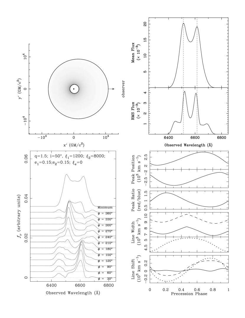
Figure 31: Elliptical disk results for a disk based on the circular disk to PKS 0921–213 ($q$=1.5, $i$=$50^{\rm\circ}$, $\xi=1200$–8000, $\sigma$=600$\;{\rm km\;s^{-1}}$) from Eracleous & Halpern (2003). For illustration, a constant eccentricity of 0.15 was used. Top left: grayscale image of the disk emissivity. Top right: mean and rms profiles. Bottom left: differences from the minimum spectrum at various precession phases. Bottom right: variations in profile parameters with precession phase. In the lower two panels, the velocity width and shift of the half-maximum are represented by solid lines, those at the quarter-maximum by dahsed lines, and the peak separation and the average peak velocity by dotted lines. See §4.2 for a description of the model parameters.

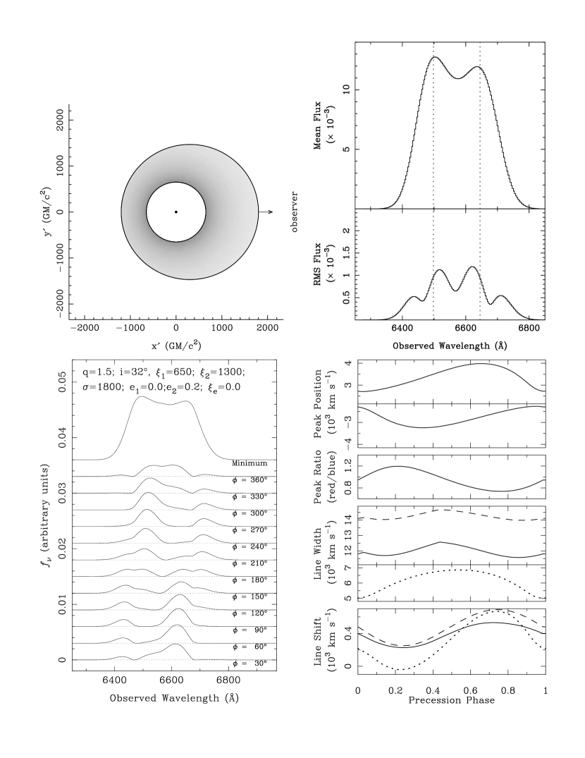
Figure 32: Similar to Figure 31, but for an elliptical disk model based on the circular disk fit to PKS 1739+18C ($q$=1.5,$i$=$32^{\rm\circ}$, $\xi$=650–1300, $\sigma$=1800$\;{\rm km\;s^{-1}}$) from Eracleous & Halpern (1994). For illustration a eccentricity which increases linearly from $e=0$ at $\xi$=650 to $e=0.2$ at $\xi_{e}$=1300 was used.

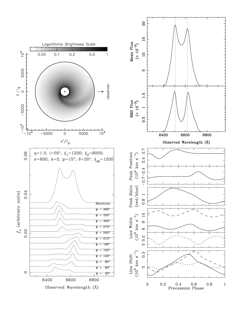
Figure 33: Similar to Figure 31, but for a model with a single, spiral arm. As with Figure 31, the circular disk parameters are based on those that best-fit PKS 0921–213. For illustration, a spiral arm with $A$=2, $p$=15^∘, $\delta$=35^∘, and $\xi_{sp}$=1200 was used.

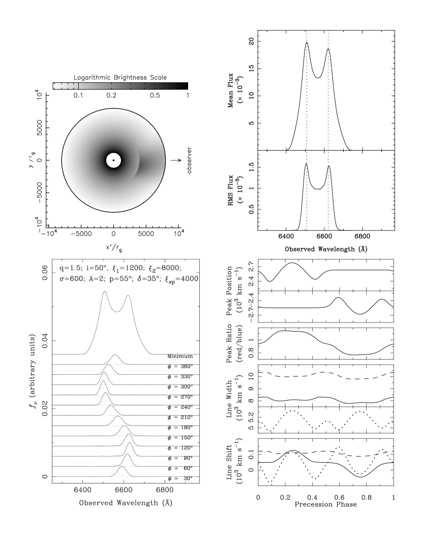
Figure 34: Similar to Figure 33 but for a spiral arm with $A$=2, $p$=55^∘, $\delta$=35^∘, and $\xi_{sp}$=4000.

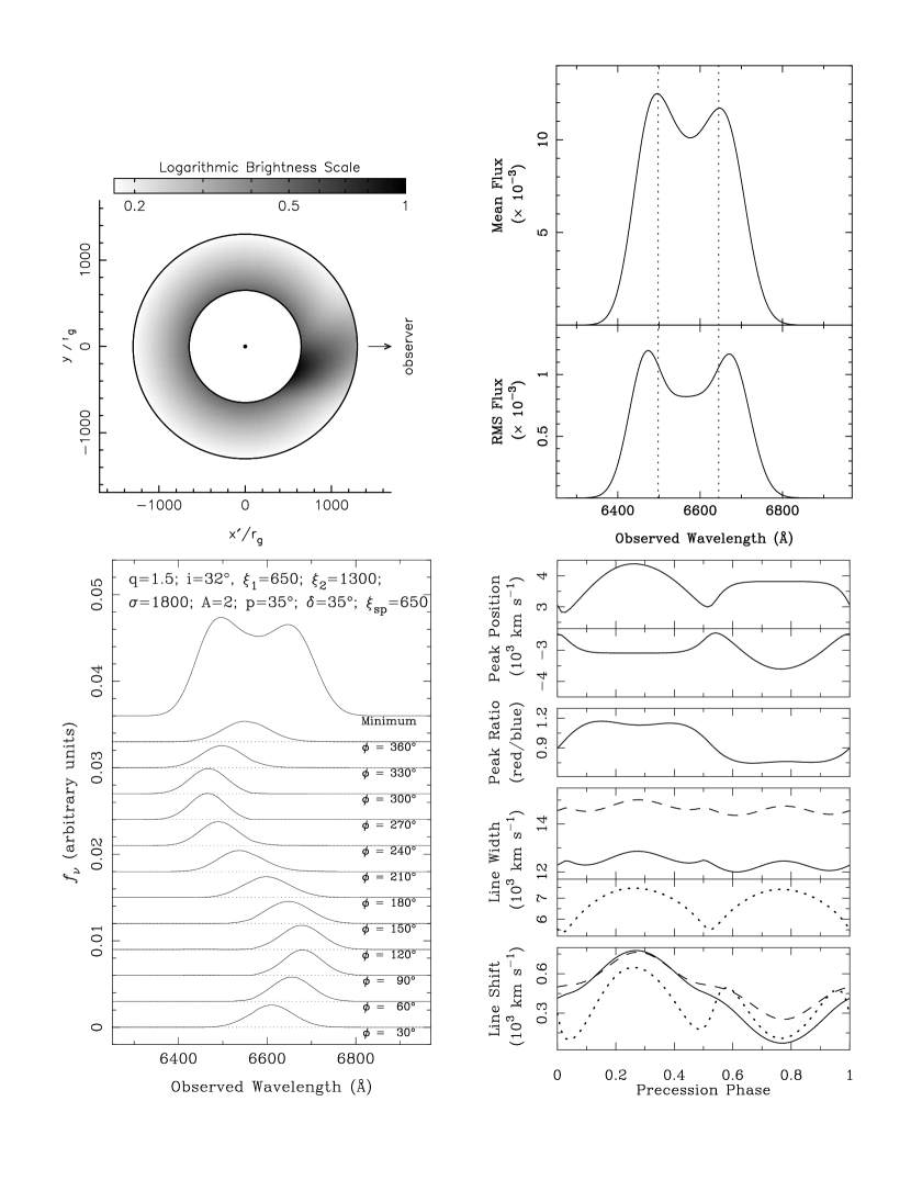
Figure 35: Similar to Figure 33 but for a circular disk based on the best-fit model for PKS 1739+18C (see Figure 32) and a spiral arm with $A$=2, $p$=35^∘, $\delta$=35^∘, and $\xi_{sp}$=650.

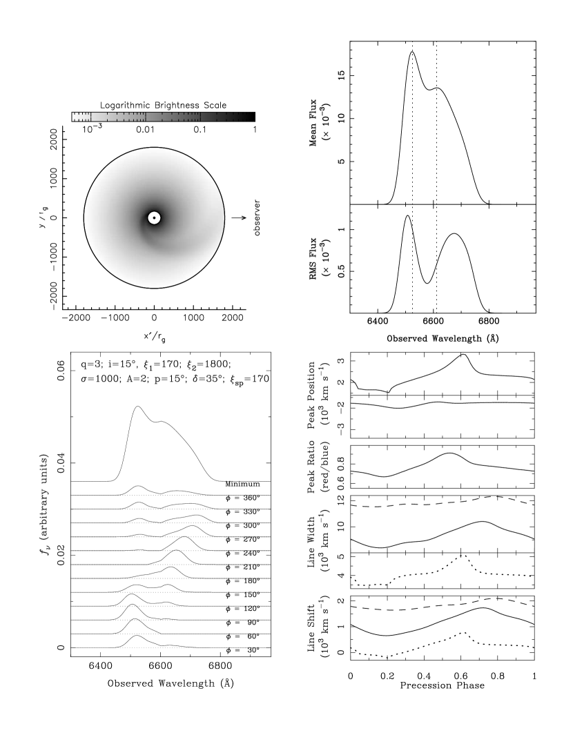
Figure 36: Similar to Figure 33 but for a circular disk based on the best-fit model for CBS 74 ($q$=3, $i$=$15^{\rm\circ}$, $\xi$=170–1800, $\sigma$=1000$\;{\rm km\;s^{-1}}$) from Eracleous & Halpern (2003) and a spiral arm with $A$=2, $p$=15^∘, $\delta$=35^∘, and $\xi_{sp}$=170.

We have characterized extensive libraries of these model profiles in exactly the same way as for the data, namely by constructing rms and difference spectra and plots of the profile parameters as a function of time. For each set of model profiles, the primary disk parameters ($\xi_{1},\xi_{2},i,q,\sigma$) were chosen to specifically match some of the objects being studied here to facilitate a comparison. In Figures 31–36 we show a few representative examples for models based on PKS 0921–213, PKS 1739+18C, and CBS 74 whose best-fit circular disk models span a range of ratios of inner to outer disk radii and inclination (Eracleous & Halpern, 1994, 2003). The other model properties were chosen simply for illustration. In each of these figures, the emissivity of the disk is shown in the top left panel. The elliptical disk model leads to qualitatively similar variability properties over a wide range of model parameters, although the amplitude of the variations is certainly dependent on specific model parameters. The spiral-arm model exhibits more diverse variability patterns thus, a larger number of examples are shown. We note that CBS 74, due to its skewed profile, does not always exhibit the same trends as the other objects.

rms spectra – see the top right panel in Figures 31–36. There is a striking difference between the rms spectra for the elliptical and spiral arm models. The elliptical disk models show two sets of peaks, with primary peaks occurring at projected velocities slightly smaller than those in the mean and a secondary set at larger projected velocities. The overall amplitude of the rms profile increases with the eccentricity, but the shape of the profile is primarily determined by the eccentricity prescription (constant versus linearly increasing) with larger primary/secondary peak ratios and more widely separated secondary peaks for constant eccentricity disks. It is also not uncommon for the red peaks of the rms profile to be stronger than the blue. The models based on CBS 74 show behavior that is fundamentally the same as the other objects, but the peak shifts are so extreme that that the red peak in the mean usually corresponds to a minimum in the rms profile.

On the other hand, the spiral-arm model produces rms profiles that are more similar to the mean profile, with just one set of peaks that are always at larger projected velocities than in the mean. The amplitude of the rms variability does not depend on any one parameter. As would be expected, the FWHM of the rms profile is larger when the spiral arm extends to small radii, however the peaks of the profile remain constant over a wide range of model parameters. The low projected velocity portion of the profile is the most sensitive to the changes in the model parameters (see Figures 33–34). However, this region is contaminated by the narrow ${\rm H\alpha}$+[N ii] lines so this is not a useful diagnostic. Again, models based on CBS 74 are somewhat different; the projected velocity of the red peak of the rms profile decreases quite dramatically as the inner radius of the spiral arm increases. Also, as with the elliptical models, the red peak in the mean usually corresponds to a minimum in the rms profile.

Difference spectra – see the bottom left panel Figures 31–36. The difference spectra for the spiral-arm models, as expected, reveal a lump of excess emission that travels across the profile. When the arm has a small pitch angle, at certain phase angles the line of sight passes through the arm at two different locations, leading to two lumps of emission at different velocities (e.g. Fig 33. However, there is typically a single lump of emission and the difference spectra are quite simple. This lump of emission changes shape (broadening and sharpening) depending on whether the line of sight passes across or along the spiral arm. The difference spectra for the elliptical disk models are comparatively complex. There are always two main lumps of emission, one blue-shifted and another red-shifted, which alternate in strength, and the stronger lump is generally narrower than the weaker lump.

Variability plots –see the bottom right panel Figures 31–36. When considering the variability plots, it is the elliptical disk model which yields extremely simple variability patterns. All of the profile parameters, with the exception of the peak separation, vary nearly in concert (i.e. the minima and maxima co-incide). Every parameter, except the profile width at HM and QM, has exactly one minimum and one maximum per precession cycle, and the profile variations occur smoothly and symmetrically. The profile widths and shifts at HM and QM often undergo very little change in comparison to the peak separation and the shift in the average velocity of the peaks. When the eccentricity is increased, or made constant throughout the disk, the only effect is to increase the amplitude of the variations.

On the other hand, the profile properties of the spiral-arm model vary in a non-uniform manner. A parameter can remain nearly constant and then undergo a significant change over a small fraction of the precession period; this is best exemplified by the velocities of the red and blue peaks. This is because the spiral arm is localized in projected velocity space. The FWHM and FWQM are the only parameters that vary at similar times and by the same magnitude. Although the shifts in the profile centroids at HM and QM tend to vary at roughly the same time, they can vary by different magnitudes. All of the models shown are for spiral arms with $A=2$ to facilitate comparison; when the amplitude is increased, the variability patterns are not qualitatively different, but the amplitude of the variations increases.

It must be noted that there are certainly instances, particularly when the pitch angle and/or arm width is large, that the spiral-arm model predicts smoothly varying profile parameters that resemble those seen from the elliptical disk models; smooth variability does not preclude a spiral arm but non-uniform variability does eliminate an elliptical disk unless additional perturbations are added.

This characterization has shown that the spiral arm and elliptical disk models are (in most instances) clearly distinguishable. Furthermore, in the case of the spiral-arm model, the variability plots are very sensitive to the input model parameters; therefore plots of this type could be extremely useful in quickly pinpointing which spiral arm parameters are most likely to reproduce a sequence of observed profiles.

5 DISCUSSION AND INTERPRETATION

5.1 Comparison of Observed Profile Variability With Models

The greatest difficulty in comparing the observed variability patterns with those predicted by the models is that the observed data need not correspond to a full precession cycle. Although this has no impact on the variability plots, it does affect the characterization of the rms and difference spectra. Therefore, for a subset of the models in our library, we constructed the rms profiles and the two comparison profiles (minimum and average) used for the difference spectra using only a quarter or half of the cycle, starting at various initial phase angles.

For the elliptical disk model, we find that the rms profile has the same basic characteristics (two sets of peaks) even when just a quarter cycle is used. On the other hand the minimum and average profiles are very different; even when using a half cycle and the difference spectra are greatly affected. However, we note that the difference spectra still have lumps of emission at both negative and positive projected velocity. For the spiral-arm model, the minimum spectrum is very robust. The minimum profile for a half-cycle is indistinguishable from that for the full cycle, and when a quarter cycle is used, the relative heights of the two peaks are affected slightly but the profile is still quite similar. The average profile is affected more than the minimum by partial cycles, but again the profiles are still quite similar to those from a full cycle. Thus for the spiral-arm model, the difference spectra presented in Figure 33–36 remain qualitatively the same even if a fraction of a cycle is used. However, the rms plot changes considerably with one of the two peaks often disappearing. Thus for the elliptical model, comparisons between the observed and predicted difference spectra should be made with extreme caution, whereas for the spiral-arm model it is the rms profiles that are subject to the greatest uncertainty. With this in mind, we now compare the most prominent observed variability trends with those predicted by the models.

rms Variability. – Neither model is very successful in reproducing the rms profiles observed, which often have three distinct features. The observed rms profiles do not have four peaks, as predicted by the elliptical disk model even for partial cycles. In some objects with peaks close to the narrow H$\alpha$+[N ii]  the inner pair of peaks could be masked by the narrow lines, but this is not the case for most objects. The spiral arm model, on the other hand, leads to rms profiles with at most two peaks (depending on what fraction of the cycle is used). Both models can account for the unusual rms profile of CBS 74, which has a red peak in the rms profile that is at a significantly larger projected velocity than the peak in the mean profile as well as a minimum in the rms profile at the velocity of the red peak in the mean profile. The behavior of PKS 1739+18C (which has a minimum in the rms profile coinciding with a peak in the mean profile) is not reproduced by either model.

Difference spectra. – The observed difference spectra show multiple lumps of excess emission, both at positive and negative projected velocity, which is consistent with the elliptical disk but disfavors a simple spiral-arm model. The spiral-arm model can only produce multiple lumps that are both red- and blueshifted at specific lines of sight through the spiral arm. However, the lumps exhibit large variations in projected velocity which is not seen in the elliptical disk models, where the two primary lumps of emission simply trade off in amplitude without the lumps drifting significantly in projected velocity. Considering that the difference spectra for the elliptical disk models are sensitive to partial cycles, the observed difference spectra could be qualitatively consistent with those predicted by the elliptical disk model.

Profile parameter variability. – Both models naturally lead to reversals in the peak flux ratio without fine-tuning, however the elliptical disk model can lead to more dramatic peak reversal than the spiral-arm model. Neither model can reproduce the large number of spectra where the red peak is stronger than the blue, and the red peak is never stronger than the blue for more than half of the cycle. Unless all of the objects were preferentially observed at a time when the red peak was stronger, neither model can explain the large fraction of observations with the red peak stronger than the blue. Both models can produce profiles that are blueshifted at times but blueshifts are more easily produced by the elliptical disk model because the variations are always symmetric. Within the parameter space explored here, extreme blue shifts (on the order of 1000 ${\rm km\;s^{-1}}$) are not easily produced. Strateva et al. (2003) explored a much wider range of parameter space for the elliptical disk model and find that such blue-shifts are completely consistent with the elliptical disk model at least. The spiral-arm model has a much larger parameter space and it has not been explored as extensively. The most distinctive characteristic of the observed profile parameter plots is the fact that the parameters do not vary in concert and the variations, although systematic, are not smooth. This disfavors the elliptical disk model, but is consistent with the spiral-arm model.

5.2 Variability Timescales

Besides the various differences in profile variability, another significant difference between these two models is the pattern precession timescale. If a spiral perturbation is triggered by the self-gravity of the disk, the resulting pattern can be expected to roughly co-rotate with the disk. Thus the variability would occur on nearly the dynamical timescale.

$$\tau_{\rm dyn}=6\;M_{8}\;\xi_{3}^{3/2}~{}{\rm months}$$ (1)

where $M_{8}$ is the mass of the black hole in units of $10^{8}\;{\rm M_{\odot}}$, $\xi_{3}$ is the radius from the center of the black hole, in units of $10^{3}\;r_{g}$.

Simulations indicate that when the disk is less massive than the central object, the disk is stable to the development of a single-armed ($m$=1) mode, however a single-armed spiral can result from the interaction between higher order perturbations.Laughlin & Korchagin (1996, and references therein). These authors find that the pattern speed will be similar to the beating frequency of these two modes; in the case of an interaction between the m=3 and m=4 modes, the expected pattern speed is about an order of magnitude longer than the dynamical timescale. Finally, a spiral arm that is externally triggered (e.g. by a binary companion) will precess on characteristic time scale associated with the perturbing object.

As described in Eracleous et al. (1995), an elliptical disk can precess due to two effects, the precession of the pericenter due to relativistic effects, which occurs on a timescale of

$$P_{\rm GR}\sim 10^{3}\;M_{8}\;\tilde{\xi}_{3}^{5/2}~{}{\rm yr}$$ (2)

or in the case of a binary, also due to the tidal forces of the secondary

$$\tau_{\rm tidal}\sim 500\left(\frac{q_{4}^{3}}{1+q_{4}}\right)\;a_{17}^{3/2}\;M_{8}^{-1/2}~{}{\rm yr}$$ (3)

where $\tilde{\xi}_{3}$ is the pericenter distance in units of $10^{3}r_{g}$, $q_{4}$ is the mass ratio divided by four, and $a_{17}$ is the binary separation in units of $10^{17}$ cm. Equation 2 is only applicable to an accretion ring (i.e. when the ratio of the outer to inner radius is small). In a large disk (and in the absence of a constant perturbing force) the inner disk will circularize before the outer disk has had an opportunity to precess significantly.

For three objects in this study, Pictor A, PKS 0921-213, and 1E 0450.3-1817, the black hole masses are known ($M_{BH}\sim 4\times 10^{7}{\rm M_{\odot}}$; Lewis & Eracleous, 2006), giving dynamical timescales of $\sim$ 1–4 months at r=1000 $r_{g}$ (where the spread is the result of a 50% uncertainty in the black hole mass). If the disk is unstable to the formation of a single-armed mode, the precession timescale could be as small as a few months. However in the more likely case of interactions between higher order modes or external perturbation, the precession timescale for a spiral arm is several years or longer. On the other hand, the expected precession timescale for the elliptical disk is 400 years! The fact that clear variability is observed within one decade in these objects strongly suggests that the elliptical disk model is untenable. Although black hole masses have not been obtained for the other objects in this study, these objects are unlikely to have black hole masses that are significantly smaller than these. The X-ray luminosities of the remaining objects are all on the order of $10^{44}\;{\rm erg\;s^{-1}}$; if the black hole masses were less than $10^{7}\;{\rm M_{\odot}}$, the X-ray luminosity alone would exceed the Eddington luminosity ($1.3\times 10^{38}\;M_{BH}/{\rm M_{\odot}}\;{\rm erg\;s^{-1}}$). Thus it appears that the elliptical disk model may not be tenable for any objects in this sample.

5.3 Refinements to the Spiral-Arm Model

Like Gezari et al. (2007) we find that neither of these simple disk models can explain the observed profile variability behavior in detail, although both account for some of the common trends. However, we must keep in mind that these models are the simplest extensions to the circular disk. There is much room for improvement and it is possible that alternatives or modifications to the above models might yield better agreement with the observed profile variability. Here, we focus on the spiral-arm model, which at least based on the variability timescale, is a viable scenario. One simple modification which has already been used successfully in NGC 1097 (Storchi-Bergmann et al., 2003) is to allow the emissivity power-law index to vary with both radius and time. However, as noted in §3.2 and §3.4, no unambiguous trends between the profile properties and broad H$\alpha$ flux were found thus, such a scenario is not justified for the objects studied here.

In the detailed descriptions of the observed difference spectra, we noted that while it was implausible that the lumps of emission were due to persistent bright spots orbiting in the disk, the non-random distribution of lumps in projected velocity strongly suggested that the various lumps were somehow physically associated with each other. There appear to be two aspects of the variability; the projected velocity of the lumps changes on long timescales, whereas the properties of the lumps can change on much shorter timescales. These two aspects of the variability might be naturally explained if the spiral arm is fragmented.

Chakrabarti & Wiita (1993) modeled spiral arms in AGN disks triggered by the close passage of another body and find that the arm does fragment and reform. Their primary motivation was to explore whether such a mechanism could explain the flux variability of AGN, and indeed they found that as an arm forms, the flux increases on timescales of a year to several years and then small 1% variations in the flux occur on timescales of several months as the arm fragments and reforms. However the simulations were limited to mass ratios of $>10^{-3}$ and it is unclear what effect the close passage of a more common stellar mass object would have or how long-lived the induced spiral arm would be. However, a molecular cloud or star cluster may be massive enough to trigger an instability.

Alternatively, the disk itself might be non-uniform with the sub-structure of the disk changing on short timescales, comparable to the dynamical timescale. For example, if the emissivity of the arm is dominated by isolated clumps that happen to be passing through the arm, this could lead to the observed variability in the amplitude and shape of the lumps while preserving the slow changes in the projected velocity of the lumps.

Flohic & Eracleous (2008) performed simulations to investigate the applicability of disks with stochastically changing bright regions to the variability of Arp 102B and 3C 390.3. They consider several mechanisms to create emissivity enhancements in the disk: self-gravitating clumps (e.g. Rice et al., 2005), hot spots generated in a collision between the disk and stars (Zurek et al., 1994), or baroclinic vortices (Petersen et al., 2007) that result from the combined effects of the temperature gradients in the disk and the differential rotation.

Goodman & Tan (2004) present estimates for the radius at which an AGN accretion disk will become marginally stable to self-gravity. Using these results, and the range of Eddington luminosities and black hole mass for Pictor A, 1E 0450.3–1817, and PKS 0921–213 presented in Lewis & Eracleous (2006), we calculate the range of radii at which the disks in these objects might become unstable, with the large range resulting primarily from uncertainty in the black hole mass. The disk of 1E 0450.3–1817 is marginally stable at radii larger than 1700–3300 $r_{g}$ whereas the disks of Pictor A and PKS 0921–213 are maringally stable at radii larger than 3100–4400 $r_{g}$. For both 1E 0450.3–1817 and PKS 0921–213 the best-fit disk parameters (Eracleous & Halpern, 1994, 2003) indicate that the region of instability is well within the line-emitting portion of the disk, thus the formation of self-gravitating clumps is a possibility for these objects. However, Pictor A has a much smaller disk and based on these estimates, the disk should be stable to self-gravity.

In all of the scenarios considered by Flohic & Eracleous (2008), the emissivity enhancements are fairly long-lived, thus one would expect such emissivity enhancements to rotate through the disk on a dynamical timescale. We do not observe such behavior in the few objects that were closely monitored. This suggests that the decay time of bright spots is shorter than the dynamical time. Alternatively, the bright spots are generated when pre-existing clumps are compressed further as they pass through the spiral arm.

With these considerations, a model in which the arm itself is undergoing fragmentation seems much more attractive as the changing emissivity pattern would naturally travel with the arm as it precesses through the disk.

The situation of having more than one lump of emission, on both sides of the profile might also be accommodated with more complex spiral arm models. Although Gilbert et al. (1999) found that multiple spiral arms led to a disk that was too axisymmetric to reproduce the observed peak reversals, this was for a uniform spiral perturbation, not one in which isolated clumps or fragments dominated the emissivity. In this scenario, there may be no observational obstacle to the presence of multiple spiral arms. There are some significant problems that this clumpy spiral-arm model does not remedy, namely the large blueshifts that are observed at times and the fact that most objects have red peaks stronger than the blue in at least 50% of the spectra.

5.4 Mass in the Lumps of Emission

A final consideration is how much mass is involved in the excess lumps of emission identified in the difference spectra. The lumps are typically 5%–10% of the total broad H$\alpha$ flux and the luminosity of the lumps ranges from $4\times 10^{40}$ to $\;2\times 10^{42}{\rm erg\;s^{-1}}$, with an average luminosity of $5\times 10^{41}{\rm erg\;s^{-1}}$, although as noted previously, the absolute luminosities are uncertain by up to a factor of 2. Assuming that the excess luminosity is due to Hydrogen recombination, one can roughly estimate the mass of Hydrogen involved, assuming constant density and temperature:

$$\frac{L_{\rm H\alpha}}{M_{\rm H\alpha}}=\frac{n_{e}\;{\rm h\nu_{H\alpha}}\;\alpha_{\rm eff,H\alpha}}{\rm m_{H}}$$ (4)

where $L_{\rm H\alpha}$ is the H$\alpha$ luminosity, $M_{\rm H\alpha}$ is the mass of hydrogen gas participating in the emission, $n_{e}$ is the electron density in ${\rm cm^{-3}}$, $\rm{m_{{\rm H}}}$ is the mass of the hydrogen atom, and $\alpha_{\rm eff,H\alpha}$ is the recombination coefficient, which we assume to be $\sim 10^{-13}\;{\rm cm^{3}s^{-1}}$, appropriate for gas with temperatures between 5000-10,000 K Osterbrock (1989, Table 2.1). We note that $M_{\rm H\alpha}$ is a lower limit to the total mass of the gas, since it is expected that only a photo-ionized skin of the matter involved will emit H$\alpha$. For an electron density of $10^{11}\;{\rm cm^{-3}}$, typical for the broad-line region (BLR; e.g., Peterson, 1997), $M_{\rm H\alpha}$ in the average lump is $\sim 0.05\;\rm{M_{\odot}}$, but the electron densities inferred for the accretion disk is $10^{13-15}\;{\rm cm^{-3}}$ (e.g., Collin-Souffrin, 1987), so the emitting mass is probably of order $10^{-4}\;{\rm M_{\odot}}$ or less. Based on comparison with the model profiles, the amplitude of the spiral emissivity pattern is probably $A\lower 2.0pt\hbox{$\;\scriptscriptstyle\buildrel<\over{\sim}\;$}1.5$ and only a 20% perturbation in density would be required. In general, we expect that very little mass is needed to produce the observed lumps of excess emission in the H$\alpha$ line profiles.

6 Summary and Conclusions

In this paper we have characterized, in a model-independent way, the variability of the broad, double-peaked H$\alpha$ emission lines in seven objects (Pictor A, PKS 0921–213, 1E 0450.3–1817, CBS 74, 3C 59, PKS 1739+18, and PKS 1020–103) which have been monitored over the past decade. As indicated by the rms profiles, the greatest variability occurs at larger projected velocities, and in particular many objects show a peak in the rms profile at large negative projected velocities. Difference spectra showed that the variability is caused primarily by discrete lumps of excess emission that change in morphology and amplitude on timescales of a few years and drift in projected velocity on longer timescales. There are often multiple lumps of emission observed at a single epoch and they are generally located at both positive and negative projected velocities. For some objects the dynamical timescale is known to be only a few months, thus these lumps cannot be orbiting bright spots such as those used to model Arp 102B (Newman et al., 1997; Sergeev et al., 2000).

The most striking profile variations observed are changes in the ratio of the red to blue peak flux, thus this trend which has long been observed in some of the better-studied double-peaked emitters is very common indeed. In fact, with the exception of CBS 74, all of the objects in this study have a red peak that is stronger than the blue in at least 50% of the observations. Some objects in this sample are very extreme, most notably PKS 0921–213 and Pictor A, in that the blue peaks, which are supposed to be boosted due to relativistic effects, are rarely observed to be stronger than the red peak. We also noted that many objects had profiles that were blue-shifted by up to 1000$\;{\rm km\;s^{-1}}$, again contrary to the expectations of the simple circular disk model. Further observation of these objects is important; should they continue to show strong red peaks and overall blueshifts this will place important constraints upon models for the broad-line region in these objects.

We compared these variability trends with those expected from two simple models, an elliptical accretion disk and a circular disk with a single-armed spiral emissivity perturbation. In general, neither of these models reproduces the observed variability trends in detail; most importantly spiral-arm models do not predict the presence of multiple lumps of emission at a single epoch and the elliptical disk model predicts profile parameters variations that are extremely smooth, uniform, and symmetric and also rms profiles with four peaks, neither of which is observed. From a consideration of physical timescales, at least for the three objects with a known black hole mass (Pictor A, PKS 0921–213, and 1E 0450.3–1817), the spiral arm models is able to produce variability on a reasonable timescale, while the eccentric disk model appears to be untenable.

Thus we propose an extension to the spiral-arm model in which one or more fragmented spiral arms are present in the accretion disk. This model retains many of the general theoretical characteristics of the simple, uniform spiral arm but is likely to produce the observed variability more successfully. This model is inherently stochastic and it will be necessary to perform simulations to determine whether, statistically, such a model can reproduce the types of behavior observed. Such work is already being undertaken, in the context of a clumpy disk by Flohic & Eracleous (2008), but has not yet been extended to the scenario proposed here. We reiterate that the models considered here are the simplest extensions to a circular disk and more sophisticated models will be required. In particular it may be important to consider an accretion disk wind or other outflow to explain the full range of behaviors that are observed.

Finally, we note that significant variability appears to be occurring on timescales of less than a year in some objects. In particular lumps of emission were observed to change significantly in shape and/or amplitude within one year, and it is quite possible that some rapid variations are being missed by the current observing strategy. It would be very useful to monitor all objects at least twice per year, and to intersperse periods of intense monitoring (perhaps as often as every few weeks) for a few of the more variable objects such as 1E 0450.3–1817 or PKS 0921–213. In particular, to test the fragmented spiral-arm model, it is necessary to determine the lower limit for the timescale over which the individual lumps of emission change in amplitude and morphology, which would provide an estimate of the fragmentation timescale.

Table 1: Galaxy Properties

Object				Starlight	$L_{X}{\rm(erg\;s^{-1})}$	X-ray
Name	$m_{V}$	$z$	E(B-V)	Fraction	(0.1–2.4 keV obs.)	Ref.
3C 59	16.0	0.1096	0.064	20%–30%	$1.6\times 10^{44}$	1
1E 0450.3-1817	17.8	0.0616	0.043	40%–50%	$5.4\times 10^{42}$	2
Pictor A	16.2	0.0350	0.043	10%	$3.9\times 10^{43}$	3
CBS 74	16.0	0.0919	0.036	10%	$2.6\times 10^{44}$	4
PKS 0921–213	16.5	0.0531	0.060	30%–40%	$3.3\times 10^{43}$	5
PKS 1020–103	16.1	0.1965	0.046	10%	$8.4\times 10^{44}$	3
PKS 1739+18C	17.5	0.1859	0.062	10%	$5.7\times 10^{44}$	3

Table 2: Instrumental Configurations

Code	Telescope	Spectrograph	Grating	Slit Width ($\arcsec$)	Spec. Res. (Å)
1a	KPNO 2.1m	GoldCam	240	1.8–1.9	4.5–5.5
1b	KPNO 2.1m	GoldCam	35	1.8–2.0	3.5–4.4
2a	KPNO 4m	RC	BL 181	1.7	6.0
3a	CTIO 1.5m	Cass	35	1.8	3.0–4.0
3b	CTIO 1.5m	Cass	26	1.8	3.5–4.0
3c	CTIO 1.5m	Cass	9	1.3	8.0
3d	CTIO 1.5m	Cass	32	1.8	6.0–7.0
4a	CTIO 4m	RC	G510	1.5–2.0	6.0–8.0
4b	CTIO 4m	RC	KPGL2	1.5	7.0–8.0
4c	CTIO 4m	RC	BL 181	1.5	1.0–2.0
4d	CTIO 4m	RC	G250	1.5	8.0
5a	Lick 3m	Kast	2	2.0	6.3
6a	MDM 1.3m	MK III	600 l/mm	1.5–2.0	5.0–6.0
7a	MDM 2.4m	Modspec	600 l/mm	1.25–1.5	4–5
7b	MDM 2.4m	Modspec	830 l/mm	1.25	2.9
8a	HET 9.2m	LRS	Grism 3	1.5	4.8
8b	HET 9.2m	LRS	Grism 1	1.0	9.3
9a	du Pont 2.5m	Boller & Chivens	BL 1200 l/mm	2.0	5.0

Table 3: Observation Log

	Exposure	Instr.
UT Date	Time (s)	Code
3C 59
1991 Feb 04	1800	2a
1991 Feb 05	1500	3a
1997 Feb 07	3000	1a
1997 Sep 28	3600	3a
1998 Oct 13	3600	3a
1998 Oct 15	3600	1a
1998 Dec 20	2400	7a
1999 Dec 04	3600	1b
2000 Sep 24	3600	1b
2001 Jul 21	2700	1b
2002 Oct 11	3600	1b
2003 Oct 21	600	8a
2004 Jan 19	600	8a
2004 Sep 09	600	8a
1E 0450.3–1817
1989 Nov 06	3600	6a
1989 Nov 07	5400	6a
1991 Feb 05	1800	2a
1992 Jan 16	7200	4a
1994 Feb 16	6000	4a
1995 Jan 23	5447	1b
1996 Feb 15	3600	1a
1996 Feb 16	5400	1b
1996 Oct 10	5400	5a
1997 Jan 02	3600	3a
1997 Jan 04	3600	3a
1997 Sep 27	5700	1a
1998 Jan 02	7200	3a
1998 Oct 15	7200	1a
1998 Dec 19	6000	7a
1999 Feb 09	3600	7a
1999 Nov 01	6600	3a
1999 Dec 02	3000	1a
1999 Dec 03	3000	1a
1999 Dec 04	3600	1b
2000 Sep 23	3600	1a
2000 Sep 24	3000	1a
2001 Jan 24	8100	3c
2003 Jan 02	7200	3a
Pictor A
1983 Aug 11	4200	9
1987 Jul 21	140000	4c
1994 Feb 18	3000	4b
1994 Dec 08	300	4
1995 Sep 29	1800	4a
1997 Jan 02	3600	3a
1998 Jan 02	3600	3a
1998 Oct 20	5400	3a
1999 Nov 01	3000	3a
1999 Nov 03	1800	3c
2001 Jan 21	3600	3a
2003 Jan 04	3600	3a
CBS 74
1998 Jan 30	3600	1b
1998 Apr 09	1200	6a
1998 Oct 14	3600	1a
1999 Feb 11	3600	6a
1999 Dec 02	3000	1a
1999 Dec 04	3000	1b
2000 Mar 14	6000	6a
2000 Sep 24	3000	1b
2001 Jan 24	1800	7a
2002 Oct 11	3600	1b
2003 Mar 25	300	8a
2003 Apr 05	300	8a
2003 Oct 24	1800	7a
2003 Dec 24	1200	8a
2004 Jan 13	300	8a
PKS 0921–213
1995 Mar 24	3000	1a
1995 Mar 25	3600	1a
1996 Feb 15	7200	1a
1996 Feb 16	3600	1b
1997 Jan 02	3600	3a
1997 Jan 04	3000	3a
1997 Mar 24	1700	6a
1998 Jan 02	4800	3a
1998 Jan 28	3600	1a
1998 Apr 07	1800	7a
1998 Apr 08	1800	7a
1998 Dec 20	3000	7a
1999 Dec 02	3000	1a
1999 Dec 03	3000	1a
2000 Mar 16	6000	6a
2001 Jan 21	6000	3a
2001 Oct 24	2000	1a
2003 Jan 02	7200	3a
PKS 1020–103
1991 Feb 04	600	2a
1991 Feb 05	2400	2a
1992 Jan 16	1800	4a
1996 Feb 16	3600	1a
1997 Jan 04	3600	3a
1998 Jan 05	3600	3a
1998 Dec 20	2400	7a
1999 Dec 04	3600	1a
2001 Jan 22	7200	3d
2003 Jan 03	6000	3d
PKS 1739+18C
1992 Jul 09	1800	2a
1996 Jun 15	3600	1b
1997 Jun 09	3600	1b
1997 Sep 28	3600	1b
1998 Apr 09	3000	7b
1998 Jun 27	3000	7a
1998 Oct 13	3600	1b
1999 Jun 15	3000	1b
2000 Jun 04	2400	1b
2000 Sep 24	2400	1b
2001 Jul 21	3000	1b
2002 Jun 14	2700	1b
2002 Oct 11	3600	1b
2003 Apr 02	300	8a
2004 Jun 22	300	8a
2004 Aug 05	300	8a

Table 4: Measured Profile Parameters

Date	Flux	V(R)	V(B)	F(R)	F(B)	F(R)/F(B)	FWHM	FWQM	V(FWHM)	V(FWQM)
(1)	(2)	(3)	(4)	(5)	(6)	(7)	(8)	(9)	(10)	(11)
3C 59
1991 Feb 04	69$\;\pm\;$ 8	2.9$\;\pm\;$0.1	–1.7$\;\pm\;$0.2	0.35$\;\pm\;$0.03	0.42$\;\pm\;$0.04	0.83$\;\pm\;$0.02	10.0$\;\pm\;$0.1	13.4$\;\pm\;$0.2	01.1$\;\pm\;$0.8	00.8$\;\pm\;$1.0
1997 Feb 07	70$\;\pm\;$20	4.0$\;\pm\;$0.1	–2.9$\;\pm\;$0.3	0.36$\;\pm\;$0.09	0.29$\;\pm\;$0.07	1.21$\;\pm\;$0.03	11.6$\;\pm\;$0.1	14.0$\;\pm\;$0.2	00.6$\;\pm\;$0.8	00.5$\;\pm\;$1.0
1997 Sep 28	65$\;\pm\;$ 8	4.1$\;\pm\;$0.1	–3.1$\;\pm\;$0.2	0.37$\;\pm\;$0.04	0.29$\;\pm\;$0.03	1.26$\;\pm\;$0.02	11.3$\;\pm\;$0.1	13.2$\;\pm\;$0.2	00.5$\;\pm\;$0.8	00.2$\;\pm\;$1.0
1998 Oct 14	70$\;\pm\;$10	4.1$\;\pm\;$0.1	–2.8$\;\pm\;$0.2	0.43$\;\pm\;$0.07	0.32$\;\pm\;$0.06	1.34$\;\pm\;$0.02	10.8$\;\pm\;$0.1	13.1$\;\pm\;$0.2	00.6$\;\pm\;$0.8	00.4$\;\pm\;$1.0
1998 Dec 20	80$\;\pm\;$10	4.0$\;\pm\;$0.1	–2.3$\;\pm\;$0.2	0.42$\;\pm\;$0.06	0.36$\;\pm\;$0.05	1.16$\;\pm\;$0.02	11.1$\;\pm\;$0.1	12.8$\;\pm\;$0.2	00.5$\;\pm\;$0.8	00.2$\;\pm\;$1.0
1999 Dec 04	90$\;\pm\;$20	4.0$\;\pm\;$0.1	–2.7$\;\pm\;$0.8	0.48$\;\pm\;$0.08	0.35$\;\pm\;$0.09	1.40$\;\pm\;$0.30	10.2$\;\pm\;$0.1	13.1$\;\pm\;$0.2	00.9$\;\pm\;$0.8	00.2$\;\pm\;$1.0
2000 Sep 24	67$\;\pm\;$ 9	4.0$\;\pm\;$0.1	–1.9$\;\pm\;$0.1	0.36$\;\pm\;$0.04	0.37$\;\pm\;$0.04	0.98$\;\pm\;$0.01	10.3$\;\pm\;$0.1	13.2$\;\pm\;$0.2	01.0$\;\pm\;$0.8	00.3$\;\pm\;$1.0
2001 Jul 21	80$\;\pm\;$10	4.0$\;\pm\;$0.1	–2.0$\;\pm\;$0.2	0.42$\;\pm\;$0.08	0.35$\;\pm\;$0.07	1.22$\;\pm\;$0.08	10.6$\;\pm\;$0.1	12.6$\;\pm\;$0.2	01.0$\;\pm\;$0.8	00.6$\;\pm\;$1.0
2002 Oct 11	90$\;\pm\;$20	3.9$\;\pm\;$0.1	–2.5$\;\pm\;$0.2	0.50$\;\pm\;$0.10	0.45$\;\pm\;$0.10	1.19$\;\pm\;$0.04	10.7$\;\pm\;$0.1	12.4$\;\pm\;$0.2	00.8$\;\pm\;$0.8	00.7$\;\pm\;$1.0
2003 Oct 21	64$\;\pm\;$ 9	4.3$\;\pm\;$0.2	–1.7$\;\pm\;$0.3	0.33$\;\pm\;$0.04	0.37$\;\pm\;$0.05	0.90$\;\pm\;$0.05	10.5$\;\pm\;$0.1	12.8$\;\pm\;$0.3	00.9$\;\pm\;$0.8	01.0$\;\pm\;$1.0
2004 Jan 19	76$\;\pm\;$ 8	4.4$\;\pm\;$0.2	–1.7$\;\pm\;$0.1	0.38$\;\pm\;$0.04	0.44$\;\pm\;$0.04	0.88$\;\pm\;$0.02	10.6$\;\pm\;$0.1	12.8$\;\pm\;$0.2	00.9$\;\pm\;$0.8	00.8$\;\pm\;$1.0
2004 Sep 09	90$\;\pm\;$10	4.1$\;\pm\;$0.2	–1.9$\;\pm\;$0.1	0.48$\;\pm\;$0.06	0.51$\;\pm\;$0.06	0.95$\;\pm\;$0.03	10.6$\;\pm\;$0.1	12.6$\;\pm\;$0.2	00.7$\;\pm\;$0.8	00.5$\;\pm\;$1.0
1E 0450.3–1817
1989 Nov 06	15$\;\pm\;$ 1	3.40$\;\pm\;$0.10	–1.80$\;\pm\;$0.30	0.050$\;\pm\;$0.020	0.070$\;\pm\;$0.030	0.67$\;\pm\;$0.04	12.9$\;\pm\;$0.3	16.7$\;\pm\;$0.5	–1.1$\;\pm\;$0.2	–0.6$\;\pm\;$0.3
1991 Feb 05	12$\;\pm\;$ 1	2.93$\;\pm\;$0.08	–1.47$\;\pm\;$0.09	0.050$\;\pm\;$0.020	0.070$\;\pm\;$0.020	0.62$\;\pm\;$0.04	11.3$\;\pm\;$0.2	14.1$\;\pm\;$0.2	–1.4$\;\pm\;$0.3	–1.2$\;\pm\;$0.2
1992 Jan 16	16$\;\pm\;$ 2	3.06$\;\pm\;$0.08	–2.37$\;\pm\;$0.07	0.070$\;\pm\;$0.010	0.090$\;\pm\;$0.020	0.76$\;\pm\;$0.04	11.2$\;\pm\;$0.1	14.1$\;\pm\;$0.2	–1.2$\;\pm\;$0.3	–0.8$\;\pm\;$0.2
1994 Feb 16	21$\;\pm\;$ 2	4.10$\;\pm\;$0.30	–4.18$\;\pm\;$0.09	0.070$\;\pm\;$0.010	0.120$\;\pm\;$0.010	0.58$\;\pm\;$0.04	12.5$\;\pm\;$0.2	15.9$\;\pm\;$0.4	–0.3$\;\pm\;$0.3	00.5$\;\pm\;$0.3
1995 Jan 23	19$\;\pm\;$ 2	4.50$\;\pm\;$1.20	–4.10$\;\pm\;$0.20	0.060$\;\pm\;$0.020	0.110$\;\pm\;$0.020	0.59$\;\pm\;$0.05	13.1$\;\pm\;$0.1	15.0$\;\pm\;$0.2	00.0$\;\pm\;$0.3	00.0$\;\pm\;$0.2
1996 Feb 15	16$\;\pm\;$ 1	3.80$\;\pm\;$0.30	–5.00$\;\pm\;$0.10	0.080$\;\pm\;$0.030	0.080$\;\pm\;$0.030	0.98$\;\pm\;$0.05	13.6$\;\pm\;$0.2	15.7$\;\pm\;$0.4	–0.7$\;\pm\;$0.2	–0.8$\;\pm\;$0.1
1996 Oct 11	17$\;\pm\;$ 3	2.80$\;\pm\;$0.10	–5.67$\;\pm\;$0.06	0.090$\;\pm\;$0.020	0.080$\;\pm\;$0.020	1.05$\;\pm\;$0.04	13.3$\;\pm\;$0.1	15.2$\;\pm\;$0.2	–1.0$\;\pm\;$0.3	–1.0$\;\pm\;$0.2
1997 Jan 03	17$\;\pm\;$ 1	2.60$\;\pm\;$0.10	–5.54$\;\pm\;$0.08	0.099$\;\pm\;$0.007	0.096$\;\pm\;$0.005	1.03$\;\pm\;$0.03	13.1$\;\pm\;$0.2	14.9$\;\pm\;$0.3	–1.2$\;\pm\;$0.2	–1.1$\;\pm\;$0.1
1997 Sep 27	27$\;\pm\;$ 2	1.50$\;\pm\;$0.40	–5.80$\;\pm\;$0.30	0.140$\;\pm\;$0.010	0.110$\;\pm\;$0.010	1.23$\;\pm\;$0.05	13.2$\;\pm\;$0.1	15.5$\;\pm\;$0.2	–1.1$\;\pm\;$0.3	–0.7$\;\pm\;$0.2
1998 Jan 02	26$\;\pm\;$ 2	2.20$\;\pm\;$0.08	–6.00$\;\pm\;$0.10	0.140$\;\pm\;$0.020	0.110$\;\pm\;$0.020	1.30$\;\pm\;$0.05	13.1$\;\pm\;$0.1	15.1$\;\pm\;$0.2	–1.0$\;\pm\;$0.3	–0.9$\;\pm\;$0.2
1998 Oct 15	23$\;\pm\;$ 2	2.90$\;\pm\;$0.30	–5.90$\;\pm\;$0.30	0.080$\;\pm\;$0.020	0.070$\;\pm\;$0.020	1.16$\;\pm\;$0.05	14.5$\;\pm\;$0.1	17.1$\;\pm\;$0.4	–0.7$\;\pm\;$0.3	–0.4$\;\pm\;$0.3
1998 Dec 19	15$\;\pm\;$ 2	3.60$\;\pm\;$0.40	–5.36$\;\pm\;$0.07	0.080$\;\pm\;$0.020	0.060$\;\pm\;$0.020	1.21$\;\pm\;$0.05	14.9$\;\pm\;$0.2	17.7$\;\pm\;$0.2	–0.6$\;\pm\;$0.3	–1.0$\;\pm\;$0.2
1999 Feb 09	22$\;\pm\;$ 4	3.50$\;\pm\;$0.10	–5.16$\;\pm\;$0.09	0.080$\;\pm\;$0.020	0.070$\;\pm\;$0.020	1.15$\;\pm\;$0.04	14.8$\;\pm\;$0.2	20.2$\;\pm\;$0.4	–0.5$\;\pm\;$0.3	00.2$\;\pm\;$0.3
1999 Nov 01	24$\;\pm\;$ 5	2.90$\;\pm\;$0.20	–4.55$\;\pm\;$0.07	0.110$\;\pm\;$0.030	0.110$\;\pm\;$0.030	0.98$\;\pm\;$0.04	15.3$\;\pm\;$0.1	20.0$\;\pm\;$0.2	–0.4$\;\pm\;$0.3	–0.2$\;\pm\;$0.2
1999 Dec 03	23$\;\pm\;$ 6	2.80$\;\pm\;$0.50	–4.40$\;\pm\;$0.30	0.110$\;\pm\;$0.040	0.120$\;\pm\;$0.040	0.93$\;\pm\;$0.04	15.5$\;\pm\;$0.5	19.4$\;\pm\;$1.0	–0.2$\;\pm\;$0.2	00.2$\;\pm\;$0.3
2000 Sep 24	26$\;\pm\;$ 5	2.60$\;\pm\;$0.30	–3.10$\;\pm\;$0.80	0.100$\;\pm\;$0.020	0.130$\;\pm\;$0.030	0.77$\;\pm\;$0.04	12.6$\;\pm\;$0.2	16.6$\;\pm\;$0.2	–0.8$\;\pm\;$0.2	–0.5$\;\pm\;$0.3
2001 Jan 24	24$\;\pm\;$ 5	2.80$\;\pm\;$0.20	–4.40$\;\pm\;$0.90	0.080$\;\pm\;$0.020	0.110$\;\pm\;$0.020	0.73$\;\pm\;$0.04	12.6$\;\pm\;$0.1	16.2$\;\pm\;$0.2	–1.1$\;\pm\;$0.3	–0.6$\;\pm\;$0.3
2003 Jan 02	26$\;\pm\;$ 6	2.50$\;\pm\;$0.10	–3.60$\;\pm\;$0.20	0.110$\;\pm\;$0.030	0.100$\;\pm\;$0.030	1.06$\;\pm\;$0.04	14.2$\;\pm\;$0.1	16.5$\;\pm\;$0.3	00.0$\;\pm\;$0.3	–0.3$\;\pm\;$0.2
Pictor A
1987 Jul 21	11$\;\pm\;$ 2	5.1$\;\pm\;$0.2	–4.14$\;\pm\;$0.08	0.041$\;\pm\;$0.008	0.017$\;\pm\;$0.004	2.44$\;\pm\;$0.06	10.88$\;\pm\;$0.09	14.06$\;\pm\;$0.09	02.5$\;\pm\;$0.1	02.0$\;\pm\;$0.2
1994 Feb 18	15$\;\pm\;$ 2	5.5$\;\pm\;$0.1	–7.36$\;\pm\;$0.07	0.048$\;\pm\;$0.007	0.043$\;\pm\;$0.007	1.11$\;\pm\;$0.04	18.10$\;\pm\;$0.40	19.84$\;\pm\;$0.09	00.0$\;\pm\;$0.2	–0.1$\;\pm\;$0.2
1994 Dec 08	14$\;\pm\;$ 2	5.9$\;\pm\;$0.2	–6.80$\;\pm\;$0.20	0.056$\;\pm\;$0.006	0.037$\;\pm\;$0.004	1.53$\;\pm\;$0.04	16.20$\;\pm\;$0.20	19.00$\;\pm\;$0.20	00.0$\;\pm\;$0.2	00.0$\;\pm\;$0.2
1995 Sep 29	14$\;\pm\;$ 2	5.1$\;\pm\;$0.2	–5.76$\;\pm\;$0.06	0.049$\;\pm\;$0.005	0.029$\;\pm\;$0.003	1.72$\;\pm\;$0.04	15.50$\;\pm\;$0.10	19.10$\;\pm\;$0.08	00.1$\;\pm\;$0.1	00.2$\;\pm\;$0.2
1997 Jan 02	14$\;\pm\;$ 2	3.7$\;\pm\;$0.3	–5.09$\;\pm\;$0.05	0.039$\;\pm\;$0.005	0.038$\;\pm\;$0.005	1.04$\;\pm\;$0.04	15.20$\;\pm\;$0.20	19.30$\;\pm\;$0.20	00.0$\;\pm\;$0.1	00.9$\;\pm\;$0.2
1998 Jan 02	14$\;\pm\;$ 1	4.8$\;\pm\;$0.6	–4.10$\;\pm\;$0.06	0.039$\;\pm\;$0.004	0.042$\;\pm\;$0.004	0.92$\;\pm\;$0.05	16.20$\;\pm\;$0.20	18.47$\;\pm\;$0.08	00.7$\;\pm\;$0.2	01.1$\;\pm\;$0.2
1998 Oct 20	10$\;\pm\;$ 1	5.5$\;\pm\;$0.1	–5.05$\;\pm\;$0.06	0.027$\;\pm\;$0.002	0.025$\;\pm\;$0.001	1.10$\;\pm\;$0.04	18.15$\;\pm\;$0.08	20.47$\;\pm\;$0.04	01.3$\;\pm\;$0.1	01.1$\;\pm\;$0.2
1999 Nov 03	08$\;\pm\;$ 1	5.2$\;\pm\;$0.2	–2.87$\;\pm\;$0.09	0.019$\;\pm\;$0.002	0.022$\;\pm\;$0.002	0.86$\;\pm\;$0.04	15.90$\;\pm\;$0.20	18.60$\;\pm\;$0.20	01.7$\;\pm\;$0.2	01.6$\;\pm\;$0.2
2001 Jan 21	06$\;\pm\;$ 1	4.9$\;\pm\;$0.3	–4.22$\;\pm\;$0.05	0.015$\;\pm\;$0.003	0.015$\;\pm\;$0.003	1.01$\;\pm\;$0.04	15.80$\;\pm\;$0.50	17.60$\;\pm\;$0.50	01.2$\;\pm\;$0.3	01.3$\;\pm\;$0.3
2003 Jan 02	06$\;\pm\;$ 1	6.8$\;\pm\;$0.2	–5string00$\;\pm\;$1string00	0.014$\;\pm\;$0.002	0.012$\;\pm\;$0.002	1.10$\;\pm\;$0.08	19string00$\;\pm\;$1string00	22.50$\;\pm\;$0.50	01.3$\;\pm\;$0.4	01.4$\;\pm\;$0.3
CBS 74
1998 Jan 30	080$\;\pm\;$20	4.0$\;\pm\;$0.1	–1.81$\;\pm\;$0.05	0.33$\;\pm\;$0.06	0.54$\;\pm\;$0.09	0.61$\;\pm\;$0.02	9.43$\;\pm\;$0.09	12.4$\;\pm\;$0.2	01.1$\;\pm\;$0.2	01.3$\;\pm\;$0.4
1998 Apr 09	090$\;\pm\;$20	3.6$\;\pm\;$0.4	–1.68$\;\pm\;$0.06	0.34$\;\pm\;$0.05	0.51$\;\pm\;$0.08	0.67$\;\pm\;$0.02	9.90$\;\pm\;$0.20	13.3$\;\pm\;$0.2	01.2$\;\pm\;$0.2	01.2$\;\pm\;$0.4
1998 Oct 14	090$\;\pm\;$10	3.7$\;\pm\;$0.2	–1.60$\;\pm\;$0.20	0.35$\;\pm\;$0.01	0.54$\;\pm\;$0.02	0.66$\;\pm\;$0.03	9.70$\;\pm\;$0.20	13.3$\;\pm\;$0.2	01.2$\;\pm\;$0.2	00.9$\;\pm\;$0.4
1999 Feb 11	072$\;\pm\;$ 9	4.3$\;\pm\;$0.4	–1.21$\;\pm\;$0.07	0.30$\;\pm\;$0.01	0.48$\;\pm\;$0.02	0.63$\;\pm\;$0.02	9.82$\;\pm\;$0.07	13.3$\;\pm\;$0.2	01.1$\;\pm\;$0.2	00.9$\;\pm\;$0.5
1999 Dec 03	090$\;\pm\;$20	3.8$\;\pm\;$0.1	–1.25$\;\pm\;$0.09	0.50$\;\pm\;$0.10	0.70$\;\pm\;$0.20	0.71$\;\pm\;$0.03	9.10$\;\pm\;$0.20	13.1$\;\pm\;$0.3	01.0$\;\pm\;$0.1	00.3$\;\pm\;$0.4
2000 Mar 16	080$\;\pm\;$10	3.7$\;\pm\;$0.1	–1.68$\;\pm\;$0.07	0.37$\;\pm\;$0.02	0.57$\;\pm\;$0.04	0.65$\;\pm\;$0.02	8.70$\;\pm\;$0.10	12.8$\;\pm\;$0.2	00.9$\;\pm\;$0.2	00.2$\;\pm\;$0.4
2000 Sep 24	080$\;\pm\;$10	3.4$\;\pm\;$0.1	–1.38$\;\pm\;$0.10	0.35$\;\pm\;$0.03	0.54$\;\pm\;$0.04	0.65$\;\pm\;$0.02	9.00$\;\pm\;$0.20	14.0$\;\pm\;$0.2	00.6$\;\pm\;$0.2	–0.5$\;\pm\;$0.4
2001 Jan 24	080$\;\pm\;$10	3.4$\;\pm\;$0.2	–1.35$\;\pm\;$0.08	0.36$\;\pm\;$0.05	0.53$\;\pm\;$0.08	0.68$\;\pm\;$0.02	9.20$\;\pm\;$0.10	13.2$\;\pm\;$0.2	00.5$\;\pm\;$0.2	00.2$\;\pm\;$0.4
2002 Oct 11	090$\;\pm\;$10	2.9$\;\pm\;$0.1	–1.41$\;\pm\;$0.09	0.43$\;\pm\;$0.03	0.61$\;\pm\;$0.04	0.69$\;\pm\;$0.02	8.70$\;\pm\;$0.10	15.2$\;\pm\;$0.2	00.3$\;\pm\;$0.2	–1.0$\;\pm\;$0.4
2003 Mar 25	100$\;\pm\;$10	2.5$\;\pm\;$0.2	–1.70$\;\pm\;$0.40	0.43$\;\pm\;$0.04	0.60$\;\pm\;$0.07	0.71$\;\pm\;$0.05	9.20$\;\pm\;$0.30	14.4$\;\pm\;$0.5	00.1$\;\pm\;$0.2	–0.1$\;\pm\;$0.5
2003 Apr 05	110$\;\pm\;$20	2.3$\;\pm\;$0.1	–1.50$\;\pm\;$0.30	0.47$\;\pm\;$0.06	0.66$\;\pm\;$0.08	0.72$\;\pm\;$0.03	9.20$\;\pm\;$0.30	14.8$\;\pm\;$0.2	00.3$\;\pm\;$0.2	–0.3$\;\pm\;$0.5
2003 Oct 24	120$\;\pm\;$20	2.7$\;\pm\;$0.2	–1.38$\;\pm\;$0.09	0.52$\;\pm\;$0.04	0.76$\;\pm\;$0.06	0.68$\;\pm\;$0.02	8.70$\;\pm\;$0.20	13.7$\;\pm\;$0.2	00.5$\;\pm\;$0.3	00.1$\;\pm\;$0.5
2003 Dec 24	090$\;\pm\;$20	2.8$\;\pm\;$0.2	–1.40$\;\pm\;$0.10	0.40$\;\pm\;$0.07	0.60$\;\pm\;$0.10	0.73$\;\pm\;$0.02	9.20$\;\pm\;$0.10	14.3$\;\pm\;$0.2	00.4$\;\pm\;$0.2	00.1$\;\pm\;$0.4
2004 Jan 13	069$\;\pm\;$ 9	2.0$\;\pm\;$0.1	–1.60$\;\pm\;$0.10	0.32$\;\pm\;$0.02	0.44$\;\pm\;$0.02	0.73$\;\pm\;$0.02	9.20$\;\pm\;$0.10	14.4$\;\pm\;$0.2	00.2$\;\pm\;$0.2	00.0$\;\pm\;$0.5
PKS 0921–213
1995 Mar 24	93$\;\pm\;$ 6	2.52$\;\pm\;$0.09	–2.69$\;\pm\;$0.05	0.69$\;\pm\;$0.03	0.68$\;\pm\;$0.03	1.03$\;\pm\;$0.02	8.26$\;\pm\;$0.05	10.95$\;\pm\;$0.06	–0.1$\;\pm\;$0.1	–0.6$\;\pm\;$0.1
1996 Feb 15	76$\;\pm\;$ 8	2.45$\;\pm\;$0.08	–2.56$\;\pm\;$0.05	0.52$\;\pm\;$0.05	0.45$\;\pm\;$0.04	1.17$\;\pm\;$0.01	9.64$\;\pm\;$0.05	12.18$\;\pm\;$0.08	–0.1$\;\pm\;$0.1	–0.4$\;\pm\;$0.1
1997 Jan 02	65$\;\pm\;$ 7	2.20$\;\pm\;$0.10	–2.70$\;\pm\;$0.20	0.46$\;\pm\;$0.04	0.37$\;\pm\;$0.03	1.26$\;\pm\;$0.04	9.15$\;\pm\;$0.08	11.50$\;\pm\;$0.07	–0.2$\;\pm\;$0.1	–0.4$\;\pm\;$0.1
1997 Mar 24	56$\;\pm\;$ 5	2.00$\;\pm\;$0.20	–2.55$\;\pm\;$0.08	0.46$\;\pm\;$0.03	0.35$\;\pm\;$0.02	1.31$\;\pm\;$0.01	8.21$\;\pm\;$0.07	10.29$\;\pm\;$0.06	–0.1$\;\pm\;$0.1	–0.2$\;\pm\;$0.1
1998 Jan 02	61$\;\pm\;$ 5	1.87$\;\pm\;$0.09	–2.27$\;\pm\;$0.04	0.43$\;\pm\;$0.03	0.41$\;\pm\;$0.03	1.06$\;\pm\;$0.01	9.23$\;\pm\;$0.04	11.49$\;\pm\;$0.04	00.0$\;\pm\;$0.1	00.2$\;\pm\;$0.1
1998 Jan 28	76$\;\pm\;$ 6	2.12$\;\pm\;$0.08	–2.12$\;\pm\;$0.07	0.50$\;\pm\;$0.03	0.46$\;\pm\;$0.03	1.09$\;\pm\;$0.02	9.18$\;\pm\;$0.05	11.67$\;\pm\;$0.04	00.1$\;\pm\;$0.1	00.2$\;\pm\;$0.1
1998 Apr 07	65$\;\pm\;$ 6	2.40$\;\pm\;$0.10	–2.58$\;\pm\;$0.10	0.41$\;\pm\;$0.03	0.37$\;\pm\;$0.03	1.11$\;\pm\;$0.02	9.77$\;\pm\;$0.06	12.20$\;\pm\;$0.08	00.0$\;\pm\;$0.1	00.0$\;\pm\;$0.1
1998 Dec 20	56$\;\pm\;$ 4	2.67$\;\pm\;$0.10	–2.39$\;\pm\;$0.05	0.35$\;\pm\;$0.02	0.35$\;\pm\;$0.02	1.00$\;\pm\;$0.02	9.63$\;\pm\;$0.04	11.90$\;\pm\;$0.04	–0.1$\;\pm\;$0.1	–0.4$\;\pm\;$0.1
1999 Dec 02	47$\;\pm\;$ 3	2.80$\;\pm\;$0.20	–2.64$\;\pm\;$0.05	0.31$\;\pm\;$0.01	0.31$\;\pm\;$0.01	1.00$\;\pm\;$0.01	9.53$\;\pm\;$0.07	11.49$\;\pm\;$0.07	00.2$\;\pm\;$0.1	–0.1$\;\pm\;$0.1
2000 Mar 16	53$\;\pm\;$ 4	2.60$\;\pm\;$0.20	–2.10$\;\pm\;$0.10	0.32$\;\pm\;$0.02	0.29$\;\pm\;$0.01	1.10$\;\pm\;$0.03	9.84$\;\pm\;$0.05	12.45$\;\pm\;$0.05	00.0$\;\pm\;$0.1	–0.4$\;\pm\;$0.1
2001 Jan 21	44$\;\pm\;$ 3	2.90$\;\pm\;$0.20	–2.65$\;\pm\;$0.07	0.30$\;\pm\;$0.02	0.27$\;\pm\;$0.01	1.08$\;\pm\;$0.02	9.64$\;\pm\;$0.05	11.81$\;\pm\;$0.04	00.0$\;\pm\;$0.1	–0.3$\;\pm\;$0.1
2001 Oct 24	51$\;\pm\;$ 6	2.88$\;\pm\;$0.08	–2.50$\;\pm\;$0.10	0.39$\;\pm\;$0.04	0.35$\;\pm\;$0.04	1.11$\;\pm\;$0.02	9.01$\;\pm\;$0.04	10.90$\;\pm\;$0.04	–0.1$\;\pm\;$0.1	–0.3$\;\pm\;$0.1
2003 Jan 02	47$\;\pm\;$ 4	2.78$\;\pm\;$0.08	–2.60$\;\pm\;$0.08	0.36$\;\pm\;$0.02	0.28$\;\pm\;$0.02	1.30$\;\pm\;$0.02	8.86$\;\pm\;$0.08	10.52$\;\pm\;$0.04	00.2$\;\pm\;$0.1	00.1$\;\pm\;$0.1
PKS 1020–103
1991 Feb 05	230$\;\pm\;$30	2.00$\;\pm\;$0.10	–2.20$\;\pm\;$0.10	1.8$\;\pm\;$0.3	1.6$\;\pm\;$0.2	1.13$\;\pm\;$0.01	8.60$\;\pm\;$0.10	10.8$\;\pm\;$0.2	00.3$\;\pm\;$0.1	00.6$\;\pm\;$0.6
1992 Jan 16	320$\;\pm\;$50	1.57$\;\pm\;$0.07	–2.94$\;\pm\;$0.06	2.3$\;\pm\;$0.3	2.1$\;\pm\;$0.3	1.12$\;\pm\;$0.01	8.52$\;\pm\;$0.04	11.0$\;\pm\;$0.1	00.3$\;\pm\;$0.1	00.7$\;\pm\;$0.6
1996 Feb 16	260$\;\pm\;$30	1.83$\;\pm\;$0.08	–2.71$\;\pm\;$0.05	1.8$\;\pm\;$0.2	1.7$\;\pm\;$0.2	1.09$\;\pm\;$0.01	8.81$\;\pm\;$0.04	11.3$\;\pm\;$0.1	00.4$\;\pm\;$0.1	00.8$\;\pm\;$0.6
1997 Jan 04	200$\;\pm\;$30	1.85$\;\pm\;$0.07	–2.74$\;\pm\;$0.05	1.4$\;\pm\;$0.2	1.3$\;\pm\;$0.2	1.02$\;\pm\;$0.02	9.31$\;\pm\;$0.04	11.0$\;\pm\;$0.1	00.6$\;\pm\;$0.1	00.6$\;\pm\;$0.6
1998 Jan 05	190$\;\pm\;$30	1.90$\;\pm\;$0.07	–2.20$\;\pm\;$0.10	1.3$\;\pm\;$0.2	1.2$\;\pm\;$0.1	1.05$\;\pm\;$0.02	9.10$\;\pm\;$0.20	11.7$\;\pm\;$0.1	00.3$\;\pm\;$0.2	00.5$\;\pm\;$0.6
1998 Dec 20	250$\;\pm\;$30	2.00$\;\pm\;$0.10	–2.84$\;\pm\;$0.06	1.7$\;\pm\;$0.2	1.6$\;\pm\;$0.2	1.05$\;\pm\;$0.01	9.22$\;\pm\;$0.04	11.3$\;\pm\;$0.1	00.5$\;\pm\;$0.1	00.7$\;\pm\;$0.6
1999 Dec 04	190$\;\pm\;$40	2.00$\;\pm\;$0.10	–2.50$\;\pm\;$0.05	1.3$\;\pm\;$0.3	1.4$\;\pm\;$0.3	0.96$\;\pm\;$0.02	8.51$\;\pm\;$0.04	11.2$\;\pm\;$0.1	00.4$\;\pm\;$0.1	00.9$\;\pm\;$0.6
2001 Jan 22	210$\;\pm\;$30	2.17$\;\pm\;$0.10	–2.62$\;\pm\;$0.07	1.4$\;\pm\;$0.2	1.4$\;\pm\;$0.2	0.96$\;\pm\;$0.02	9.03$\;\pm\;$0.04	11.4$\;\pm\;$0.1	00.5$\;\pm\;$0.1	00.8$\;\pm\;$0.6
2003 Jan 03	180$\;\pm\;$20	2.20$\;\pm\;$0.30	–2.64$\;\pm\;$0.07	1.1$\;\pm\;$0.1	1.2$\;\pm\;$0.1	0.95$\;\pm\;$0.03	9.37$\;\pm\;$0.05	11.8$\;\pm\;$0.1	00.2$\;\pm\;$0.1	00.7$\;\pm\;$0.6
PKS 1739+18C
1992 Jul 09	240$\;\pm\;$020	3.45$\;\pm\;$0.08	–2.17$\;\pm\;$0.09	0.91$\;\pm\;$0.05	1.14$\;\pm\;$0.07	0.80$\;\pm\;$0.01	12.81$\;\pm\;$0.06	15.84$\;\pm\;$0.07	–0.1$\;\pm\;$0.1	–0.4$\;\pm\;$0.1
1996 Jun 15	450$\;\pm\;$040	3.22$\;\pm\;$0.07	–3.60$\;\pm\;$0.10	2.00$\;\pm\;$0.10	2.00$\;\pm\;$0.10	1.02$\;\pm\;$0.01	13.26$\;\pm\;$0.07	15.95$\;\pm\;$0.05	00.1$\;\pm\;$0.1	–0.1$\;\pm\;$0.1
1997 Jun 09	590$\;\pm\;$050	3.50$\;\pm\;$0.06	–2.70$\;\pm\;$0.20	2.70$\;\pm\;$0.20	2.60$\;\pm\;$0.20	1.03$\;\pm\;$0.02	13.50$\;\pm\;$0.10	15.82$\;\pm\;$0.07	00.2$\;\pm\;$0.1	–0.2$\;\pm\;$0.1
1997 Sep 28	580$\;\pm\;$050	3.74$\;\pm\;$0.08	–2.40$\;\pm\;$0.70	2.70$\;\pm\;$0.20	2.50$\;\pm\;$0.20	1.07$\;\pm\;$0.04	12.93$\;\pm\;$0.06	15.63$\;\pm\;$0.08	00.2$\;\pm\;$0.1	–0.3$\;\pm\;$0.1
1998 Apr 09	450$\;\pm\;$050	3.66$\;\pm\;$0.06	–2.10$\;\pm\;$0.70	2.20$\;\pm\;$0.20	2.10$\;\pm\;$0.20	1.06$\;\pm\;$0.06	13.18$\;\pm\;$0.08	15.68$\;\pm\;$0.07	00.3$\;\pm\;$0.1	–0.2$\;\pm\;$0.1
1998 Jun 27	440$\;\pm\;$070	3.65$\;\pm\;$0.07	–2.40$\;\pm\;$0.60	1.90$\;\pm\;$0.30	2.00$\;\pm\;$0.30	0.99$\;\pm\;$0.05	13.30$\;\pm\;$0.20	16.30$\;\pm\;$0.10	00.1$\;\pm\;$0.1	–0.3$\;\pm\;$0.1
1998 Oct 13	410$\;\pm\;$080	3.51$\;\pm\;$0.07	–2.40$\;\pm\;$0.50	1.90$\;\pm\;$0.30	1.90$\;\pm\;$0.40	1.00$\;\pm\;$0.04	12.90$\;\pm\;$0.30	15.70$\;\pm\;$0.10	00.3$\;\pm\;$0.2	–0.4$\;\pm\;$0.1
1999 Jun 15	360$\;\pm\;$090	3.69$\;\pm\;$0.09	–1.40$\;\pm\;$0.20	1.60$\;\pm\;$0.40	1.70$\;\pm\;$0.40	0.96$\;\pm\;$0.01	13.09$\;\pm\;$0.07	16.34$\;\pm\;$0.05	00.3$\;\pm\;$0.2	00.0$\;\pm\;$0.1
2000 Jun 04	420$\;\pm\;$090	3.50$\;\pm\;$0.10	–3string00$\;\pm\;$1string00	2.10$\;\pm\;$0.40	1.80$\;\pm\;$0.40	1.13$\;\pm\;$0.08	12.00$\;\pm\;$0.20	15.40$\;\pm\;$0.09	00.2$\;\pm\;$0.1	–0.2$\;\pm\;$0.2
2000 Sep 24	600$\;\pm\;$100	3.22$\;\pm\;$0.07	–1.70$\;\pm\;$0.10	2.90$\;\pm\;$0.50	2.80$\;\pm\;$0.50	1.04$\;\pm\;$0.02	11.90$\;\pm\;$0.20	15.70$\;\pm\;$0.20	00.4$\;\pm\;$0.1	00.0$\;\pm\;$0.1
2001 Jul 21	520$\;\pm\;$100	2.91$\;\pm\;$0.06	–2.50$\;\pm\;$0.60	2.70$\;\pm\;$0.70	2.30$\;\pm\;$0.60	1.19$\;\pm\;$0.06	11.60$\;\pm\;$0.10	14.60$\;\pm\;$0.30	00.2$\;\pm\;$0.1	00.0$\;\pm\;$0.2
2002 Jun 14	430$\;\pm\;$050	2.92$\;\pm\;$0.08	–3string00$\;\pm\;$1string00	2.40$\;\pm\;$0.20	1.90$\;\pm\;$0.20	1.30$\;\pm\;$0.10	11.50$\;\pm\;$0.10	14.38$\;\pm\;$0.08	00.3$\;\pm\;$0.2	00.1$\;\pm\;$0.2
2002 Oct 11	380$\;\pm\;$100	2.63$\;\pm\;$0.06	–2.60$\;\pm\;$0.70	2.20$\;\pm\;$0.60	1.80$\;\pm\;$0.50	1.23$\;\pm\;$0.07	11.50$\;\pm\;$0.10	14.38$\;\pm\;$0.06	00.4$\;\pm\;$0.1	00.1$\;\pm\;$0.1
2003 Apr 02	370$\;\pm\;$040	2.70$\;\pm\;$0.40	–3string00$\;\pm\;$1string00	1.90$\;\pm\;$0.20	1.70$\;\pm\;$0.20	1.12$\;\pm\;$0.07	12.19$\;\pm\;$0.07	15.10$\;\pm\;$0.10	00.2$\;\pm\;$0.2	–0.1$\;\pm\;$0.2
2004 Jun 22	250$\;\pm\;$050	3.30$\;\pm\;$0.40	–2.80$\;\pm\;$0.70	1.10$\;\pm\;$0.20	1.20$\;\pm\;$0.20	0.96$\;\pm\;$0.02	13.00$\;\pm\;$0.30	15.70$\;\pm\;$0.20	00.2$\;\pm\;$0.1	–0.3$\;\pm\;$0.1
2004 Aug 05	320$\;\pm\;$050	2.80$\;\pm\;$0.40	–2.50$\;\pm\;$0.30	1.50$\;\pm\;$0.20	1.40$\;\pm\;$0.20	1.01$\;\pm\;$0.03	12.80$\;\pm\;$0.10	15.90$\;\pm\;$0.20	00.2$\;\pm\;$0.1	00.0$\;\pm\;$0.1

Note. — Col. (1): UT Date of Observation. When multiple spectra from one observing run are averaged, the average date is listed. Col. (2): Total broad line flux divided by the [O i]$\lambda 6300$ line flux. Col. (3): Velocity of the red peak in units $10^{3}\;{\rm km\;s^{-1}}$ with respect to the narrow H$\alpha$ line. Col. (4): Velocity of the blue peak in units of $10^{3}\;{\rm km\;s^{-1}}$ with respect to the narrow H$\alpha$ line. Col. (5): Flux density ($f_{\nu}$ in mJy) at the red peak, relative to the [O i] flux. Col. (6): Flux density ($f_{\nu}$ in mJy) at the blue peak, relative to the [O i] flux. Col. (7) Ratio of the flux density of the red and blue peaks. Note that the fractional error on the ratio is much smaller than the fractional errors on the peak fluxes, because the error in the [O i] flux does not contribute. Col. (8): Full Width and Half-Maximum (defined by higher of the peaks) in units of $10^{3}\;{\rm km\;s^{-1}}$. Col. (9): Full Width and Quarter-Maximum (defined by higher of the peaks) in units of $10^{3}\;{\rm km\;s^{-1}}$. Col. (10): Velocity shift of the profile at the Half-Maximum in units $10^{3}\;{\rm km\;s^{-1}}$ with respect to the narrow H$\alpha$ line. Col. (11): Velocity shift of the profile at the Quarter-Maximum in units $10^{3}\;{\rm km\;s^{-1}}$ with respect to the narrow H$\alpha$ line. Please see §3.4 for a decsription of the measurement method and errors.

Figure 1: Plot of temporal coverage for the seven objects in this study. Each vertical bar indicates an observation described in Table 3.

Figure 2: Observed double-peaked Balmer line profiles of 3C 59, after continuum subtraction. The spectra have been scaled such that the narrow line flux is constant, so as to show the relative changes in the total broad-line flux. Arbitrary vertical offsets have been applied for clarity.

Figure 3: Same as Figure 2, but for 1E 0450.3–1817.

Figure 4: Same as Figure 2, but for Pictor A.

Figure 5: Same as Figure 2, but for CBS 74.

Figure 6: Same as Figure 2, but for PKS 0921–213.

Figure 7: Same as Figure 2, but for PKS 1020-103.

Figure 8: Same as Figure 2, but for PKS 1739+18C. The vertical dotted line indicates the position of the telluric B-band whose correction is sometimes imperfect.

Figure 14: Plot of ${\rm F_{broad\;H\alpha}}/{\rm F_{[O\;I]}}$ versus the normalized continuum flux integrated over the wavelength interval of 6635–6655Å (i.e. $\int f_{\lambda}\;d\lambda/{\rm F_{broad\;H\alpha}}$).

Figure 24: Variations in the profile properties or 3C 59: (1) the total broad-line flux, relative to [O i]$\lambda 6300$; (2) the velocity shift of the red and blue peaks, (3) the ratio of the red to blue peak flux; (4) the full-widths at half and quarter maximum and the peak separation (denoted by open triangles, filled circles, and filled black stars, respectively); (5) and the velocity shift of the profile at the HM, QM and the offset of the average peak velocity with the same symbols as for the widths. All velocities are relative to the narrow H$\alpha$ emission line. The measurement procedure is described in §3.4.

Figure 25: Same as Figure 26, but for 1E 0450.3–1817.

Figure 26: Same as Figure 24, but for Pictor A.

Figure 27: Same as Figure 24, but for CBS 74.

Figure 28: Same as Figure 24, but for PKS 0921–213.

Figure 29: Same as Figure 24, but for PKS 1020–103.

Figure 30: Same as Figure 24, but for PKS 1739+18C.

References

- Adams et al. (1989) Adams, F. C., Ruden, S. P., & Shu, F. H. 1989, ApJ, 347, 959
- Bade (1998) Bade, N. et. al. 1998, A&AS, 127, 145
- Baldwin & Stone (1984) Baldwin, J. A., & Stone, R. P. S. 1984, MNRAS, 206, 241
- Baptista et al. (2005) Baptista, L., R. Morales-Rueda, Harlaftis, E. T., Marsch, T. R., & Steeghs, D. 2005, A&A, 444, 201
- Barth et al. (2001) Barth, A. J., Ho, L. C., Filippenko, A. V., Rix, H., & Sargent, W. L. W. 2001, ApJ, 546, 205
- Begelman et al. (1980) Begelman, M. C., Blandford, R. D., & Rees, M. J. 1980, Nature, 287, 307
- Bower et al. (1996) Bower, G. A., Wilson, A. S., Heckman, T. M., & Richstone, D. O. 1996, AJ, 111, 1901
- Brinkmann et al. (1994) Brinkmann, W., Siebert, J., & Boller, T. 1994, A&A, 281, 355
- Brinkmann et al. (1995) Brinkmann, W., Siebert, J., Reich, W., Fuerst, E., Reich, P., Voges, W., Truemper, J., & Wielebinski, R. 1995, A&AS, 109, 147