An Iteratively Decodable Tensor Product Code with Application to Data Storage

Abstract

The error pattern correcting code (EPCC) can be constructed to provide a syndrome decoding table targeting the dominant error events of an inter-symbol interference channel at the output of the Viterbi detector. For the size of the syndrome table to be manageable and the list of possible error events to be reasonable in size, the codeword length of EPCC needs to be short enough. However, the rate of such a short length code will be too low for hard drive applications. To accommodate the required large redundancy, it is possible to record only a highly compressed function of the parity bits of EPCC’s tensor product with a symbol correcting code. In this paper, we show that the proposed tensor error-pattern correcting code (T-EPCC) is linear time encodable and also devise a low-complexity soft iterative decoding algorithm for EPCC’s tensor product with $q$-ary LDPC (T-EPCC-$q$LDPC). Simulation results show that T-EPCC-$q$LDPC achieves almost similar performance to single-level $q$LDPC with a $1/2$ KB sector at $50\%$ reduction in decoding complexity. Moreover, $1$ KB T-EPCC-$q$LDPC surpasses the performance of $1/2$ KB single-level $q$LDPC at the same decoder complexity.

I Introduction

The advent of high recording density enabling technologies, pioneered by galloping improvements in head and media design and manufacturing processes, has pushed for similar advances in read channel design and error correction coding, driving research efforts into developing channel-capacity-approaching coding schemes based on soft iterative decoding that are also implementation friendly [1, 2]. Soft decodable error correction codes (ECC), mainly low density parity check (LDPC) codes, would eventually replace conventional Reed-Solomon (RS) outer ECC, which despite its large minimum distance, possesses a dense parity check matrix that does not lend itself easily to powerful belief propagation (BP) decoding. There exists vast literature on the various design aspects of LDPC coded systems for magnetic recording applications. This includes code construction [3, 4, 5, 6], efficient encoding [7, 8], decoder optimization [9, 10, 11], and performance evaluation [12, 14, 13]. In this work, we propose an LDPC coded system optimized for the magnetic recording channel that spans contributions in most of these areas.

The error-pattern correcting code (EPCC) is proposed in [15, 16, 17] motivated by the well-known observation that the error rate at the channel detector output of an ISI channel is dominated by a few specific known error cluster patterns. This is due to the fact that the channel output energies associated with these error patterns are smaller than those of other patterns. A multiparity cyclic EPCC was first described in[16], with an RS outer ECC, possessing distinct syndrome sets for all such dominant error patterns. To reduce the code rate penalty, which is a severe SNR degradation in recording applications, a method to increase the code rate was introduced in [17] that also improved EPCC’s algebraic single and multiple error-pattern correction capability. In this method, the generator polynomial of the short base EPCC is multiplied by a primitive polynomial that is not already a factor of the generator polynomial. Also, the primitive polynomial degree is chosen so as to achieve a certain desired codeword length. Moreover, [17] describes a Viterbi detection postprocessor that provides error-event-reliability information aiding syndrome-mapping of EPCC to improve its correction accuracy. However, improving the EPCC code rate by extending its codeword length increases the probability of multiple dominant error patterns within the codeword, and this requires increasing the size of the syndrome table considerably to maintain the same correction power, which eventually results in prohibitive decoding complexity. To maintain correction power with a manageable size syndrome decoding table, [18] discusses a more efficient method based on a list decoding strategy that delivers satisfactory sector error rate (SER) gain with an outer RS ECC. Later, this list decoding scheme was formulated as a soft-input soft-output block in [19] and utilized to enhance the performance of turbo equalization based on convolutional codes (CC). Nevertheless, the serial concatenation scheme that proved successful with RS hard decoding and CC-based turbo equalization does not work as well in serial concatenation of long-EPCC and LDPC. The reason is that when the LDPC decoder fails, especially in the water-fall region, the sector contains a large number of multiple error occurrences. When many such error events occur in a given EPCC codeword, decoding by any reasonable size list decoder is formidable. Thus, an inner EPCC cannot in any capacity reduce the SER of a serially concatenated outer LDPC. On the other hand, if the EPCC codeword length is decreased substantially, then the number of errors per codeword is reasonable, as long as the overall code rate is somehow kept high. Here, the concept of tensor product construction comes into play.

Tensor product parity codes (TPPC) were first proposed in [21] as the null-space of the parity check matrix resulting from the tensor product of two other parity check matrices corresponding to a variety of code families. As a result, based on the choice of the concatenated codes, TPPC would be classified as an error correction code if constructed from two ECCs, an error detection code (EDC) if constructed from two EDCs, and an error location code (ELC) if constructed from an EDC and an ECC in a special order. As a matter of fact, ELCs were introduced earlier in [24] and their algebraic properties studied in detail, but later incorporated in the unified theme of TPPCs in [21]. Furthermore, a generalized class of hard-decodable ELCs was later suggested for application in the magnetic recording channel in [25]. In addition, TPPCs can be generalized by combining a number of codes on various extension fields with shorter binary codes. For this more general case, a decoding algorithm was developed in [26]. An ECC-type TPPC was applied to longitudinal magnetic recording in [22], and to perpendicular magnetic recording in [23]. In [22], a hard decodable tensor product code based on a single parity code and a BCH code is proposed as an inner code for RS. This code is suitable for low density longitudinal recording channels for which dominant errors have odd weights, such as $\{+\}$ and $\{+,-,+\}$. Also, [22] proposes that the hard decoder passes the corrected parity bits to a Viterbi detector reflecting channel states and parity code states in order to compute the decoder output. Later, [23] presented two methods for combining a tensor-product single parity code with a distance-enhancing constrained code. This code combination achieved more satisfactory performance with RS as an outer code in high density perpendicular recording channels.

Our goal in this work is to utilize the concept of tensor product concatenation to construct high rate soft-decodable EPCCs on the symbol-level of the outer ECC. The EPCC target error list is matched to the dominant error events normally observed in high density perpendicular recording channels. Since dominant error events in perpendicular recording are not only of odd weight [12], this requires that our EPCC be a multiparity code. However, in this case, a Viterbi detector matching the channel and parity will have prohibitive complexity. In spite of this, the performance of the optimal decoder of the baseline parity-coded channel can be approached by the low complexity detection postprocessing technique in [18]. We also present in detail a low complexity highly parallel soft decoder for T-EPCC and show that it achieves a better performance-complexity tradeoff compared to conventional iterative decoding schemes.

I-A Notations and Definitions

• For a linear code $C:(n,k,p)$, $n$ denotes the codeword length, $k$ denotes the user data length, and $p=n-k$ denotes the number of code parity bits.

• For a certain parity check matrix $H$ corresponding to a linear code $\{C:Hc^{t}=0,\ \forall c\in C\}$, a syndrome $s$ is the range of a perturbation of a codeword $H(c+e)^{t}=s$. A signature refers to the range under $H$ for any bit block, not necessarily a codeword formed of data and parity bits.

• The multilevel log-likelihood ratio (mlLLR) of a random variable $\beta\in GF(q)$ corresponding to the p.m.f. (probability mass function) $p_{i}(\beta)=\mathrm{Pr}(\beta=i),\sum_{i=0}^{q-1}p_{i}(\beta)=1$, can be defined as: $\gamma(\beta=i)=\log(\frac{p_{i}(\beta)}{p_{0}(\beta)}),\gamma(\beta=0)=0$.

• $[\textbf{x}]_{i}^{j}$ denotes a local segment $[x_{i},x_{i+1},...,x_{j}]$ of the sequence $x_{k}$.

• The period of a generator polynomial on $GF(2)$ corresponding to a linear code is equal to the order of that polynomial, as defined in [36]. Also, for a syndrome set $\{s^{(i)}\}_{i=0}^{L-1}$ that corresponds to all the $L$ possible starting positions of an error event, the period $P$ is defined as the smallest integer such that $s^{(\rho+P)}=s^{(\rho)}$ [18].

• Assume $\alpha_{L}=\log(\alpha)$ and $\beta_{L}=\log(\beta)$, then $(\alpha+\beta)_{L}=\log(e^{\alpha_{L}}+e^{\beta_{L}})$. Define $max^{*}\left(\begin{array}[]{*{1}c}\alpha_{L}\\ \beta_{L}\end{array}\right)=(\alpha+\beta)_{L}=\max(\alpha_{L},\beta_{L})+\log(1+e^{-|\alpha_{L}-\beta_{L}|})$. Also, $max^{*}\left(\left\{\gamma_{k}\right\}_{k=a}^{b}\right)$ and $\mathop{max^{*}}\limits_{k=a}^{b}\left(\gamma_{k}\right)$ are two different representations of the recursive implementation of $max^{*}$ acting on the elements of the set $\{\gamma_{k}\}_{k=a}^{b}$.

I-B Acronyms

• TPPC: Tensor Product Parity Code.

• $q$LDPC: $q$-ary Low Density Parity Check code.

• RS: Reed Solomon code.

• BCJR: Bahl-Cocke-Jelinek-Raviv .

• T-EPCC: Tensor product Error Pattern Correction Code.

• T-EPCC-$q$LDPC and T-EPCC-RS: Tensor product of EPCC and $q$LDPC or RS, respectively.

• LLR: Log-Likelihood Ratio.

• mlLLR: multi-level Log-Likelihood Ratio.

• ML: Maximum Likelihood.

• MAP: Maximum A Posteriori.

• QC: Quasi-Cyclic.

• SPA: Sum-Product Algorithm.

II Review of EPCC and the Tensor Product Coding Paradigm

In this section we give a brief review on the concept of EPCC, including the design of two example codes that will be utilized later in the simulation study. Also, we review the tensor product coding paradigm and present an encoding method that allows for EPCC-based linear-time-encodable TPPCs.

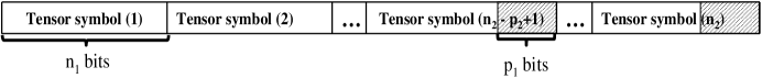
Figure 1: TPPC $C_{1}(n_{1},k_{1},p_{1})\otimes C_{2}(n_{2},k_{2},p_{2})$ codeword structure

II-A EPCC Review and Examples

We review constructing a cyclic code targeting the set of $l_{max}$ dominant error events

$$\{e^{(1)}_{k}(x),e^{(2)}_{k}(x),...,e^{(l_{max})}_{k}(x)\}$$

represented as polynomials on $GF(2)$ that can occur at any starting position $k$ in a codeword of length $l_{T}$. A syndrome of error type $e^{(i)}(x)$ at position $k$ is defined as $s^{(i)}_{k}(x)\equiv e^{(i)}_{k}(x)\ \mathbf{mod}\ g(x)$, where $g(x)$ is the generator polynomial of the code and $\mathbf{mod}$ is the polynomial modulus operation.

A syndrome set $\mathbf{S}^{(i)}$ for error type $e^{(i)}(x)$ contains elements corresponding to all cyclic shifts of polynomial $e^{(i)}(x)$; elements of $\mathbf{S}^{(i)}$ are thus related by $s_{k+j}^{(i)}=x^{j}s_{k}^{(i)}\ \mathbf{mod}\ g(x)$.

For unambiguous decoding of $e^{(i)}(x)$ and $e^{(j)}(x)$, $\forall\{i,j\}$, we must have $\mathbf{S}^{(i)}\cap\mathbf{S}^{(j)}=\oslash$. This design requirement constrains $g(x)$ to have distinct greatest common divisors with $e^{(i)}(x)$, for all targeted $i$ [16]. However, even if this constraint is satisfied, an element in $\mathbf{S}^{(i)}$ can still map to more than one error position, i.e., the period of the syndrome set- and period of $g(x)$- can be less than $l_{T}$. Moreover, this constraint is only sufficient but not necessary. As shown in [16], there may exist a lower degree $g(x)$ that can yield distinct syndrome sets for the targeted error polynomials, resulting in a higher rate EPCC. A search method to find this $g(x)$ is already discussed in detail in  [16] and [18]. We next give two example EPCC constructions that will be used throughout the paper. We target the dominant error events of the “ideal” equalized monic channel $1+0.85D$ in AWGN, which is suitable as a partial response target in perpendicular magnetic recording read channels. For this channel, the dominant errors are given by: $e^{(1)}(x)=1$, $e^{(2)}(x)=1+x$, $e^{(3)}(x)=1+x+x^{2}$, etc., i.e. they can be represented as polynomials on $GF(2)$ for which all powers of $x$ have nonzero coefficients. The two EPCCs are:

• Example 1: Targeting error polynomials up to degree $4$, we get the generator polynomial $g(x)=1+x+x^{3}+x^{5}+x^{6}$ of period $12$ via the search procedure of [16]. Choosing a codeword length of $12$, $5$ distinct, non-overlapping syndrome sets are utilized to distinguish the $5$ target errors. Then, syndrome set $\mathbf{S}^{(3)}$ will have period $6$, while all other sets have period $12$. A syndrome set of period $6$ means that each syndrome decodes to one of $2$ possible error positions within the $12$-bit codeword. Nonetheless, $e^{(3)}(x)$ can be decoded reliably via channel reliability information and the polarity of data support. The low code rate of $0.5$ makes this code unattractive as an inner code in a serial concatenation setup for recording channel applications. However, as we will see later, a tensor code setup makes it practical to use such powerful codes for recording applications.

• Example 2: Targeting error polynomials up to degree $9$, we have to record more redundancy. To accomplish this feat, a cyclic code with $8$ parity bits, code rate $0.56$, and a generator polynomial $g(x)=1+x^{2}+x^{3}+x^{5}+x^{6}+x^{8}$ of period $18$ is found by the search procedure in [16]. Then, syndrome sets $\mathbf{S}^{(1)}$, $\mathbf{S}^{(3)}$, $\mathbf{S}^{(5)}$, and $\mathbf{S}^{(7)}$ each have period $18$ and thus can be decoded without ambiguity. While syndrome sets $\mathbf{S}^{(2)}$, $\mathbf{S}^{(4)}$, $\mathbf{S}^{(6)}$, $\mathbf{S}^{(8)}$, and $\mathbf{S}^{(10)}$ each have period $9$, decoding to one of two positions. The worst is $\mathbf{S}^{(9)}$ of period $2$, which would decode to one of $9$ possible positions. Still, the algebraic decoder can quickly shrink this number to few positions by checking the data support, and then would choose the one position with highest local reliability.

II-B Tensor Product Parity Codes

II-B1 Construction and Properties of the TPPC Parity Check Matrix

Consider a binary linear code $C_{1}:(n_{1},k_{1},p_{1})$ derived from the null space of parity check matrix $H_{c_{1}}$, and assume $C_{1}$ corrects any error event that belongs to class $\varepsilon_{1}$. Also, consider a non-binary linear code $C_{2}:(n_{2},k_{2},p_{2})$ derived from the null space of parity check matrix $H_{c_{2}}$ and defined over elements of $GF(2^{p_{1}})$. Moreover, assume this code corrects any symbol error type that belongs to class $\varepsilon_{2}$. As a preliminary step, convert the binary $p_{1}\times n_{1}$ matrix $H_{c_{1}}$, column by column, into a string of $GF(2^{p_{1}})$ elements of dimension $1\times n_{1}$. Then, construct the matrix

$$H_{c_{3}}=H_{c_{1}}\otimes H_{c_{2}}$$

as a $p_{2}\times n_{1}n_{2}$ array of $GF(2^{p_{1}})$ elements. Finally, convert the elements of $H_{c_{3}}$ into $p_{1}$-bit columns, based on the same primitive polynomial of degree $p_{1}$ used all over in the construction method. The null space of the $p_{1}p_{2}\times n_{1}n_{2}$ binary $H_{c_{3}}$ corresponds to a linear binary code $C_{3}:(n_{1}n_{2},k_{3},p_{1}p_{2})$. As shown in Fig. 1, a $C_{3}$ codeword is composed of $n_{2}$ blocks termed “tensor-symbols”, each having $n_{1}$ bits. Also, it can be shown that $C_{3}$ can correct any collection of tensor symbol errors belonging to class $\varepsilon_{2}$, provided that all errors within each tensor symbol belong to class $\varepsilon_{1}$ [21]. Note that a tensor symbol is not an actual $C_{1}$ codeword, and as such, using the terms “inner” and “outer” codes would not be completely accurate. In addition, the tensor symbols are not codewords themselves, as can be seen in Fig. 1, the first $k_{2}$ tensor symbols are all data bits to start with, and even the last $p_{2}$ tensor symbols, which are composed of data and parity bits, have non-zero syndromes under $H_{c_{1}}$. Thus, a TPPC codeword does not correspond directly to either $H_{c_{1}}$ or $H_{c_{2}}$, and as a result, the component codebooks they describe are not recorded directly on the channel. Another interesting property of the resulting TPPC is that the symbol-mapping of the sequence of tensor-symbol signatures under $H_{c_{1}}$ forms a codeword of $C_{2}$, which we refer to as the “signature-correcting component code”.

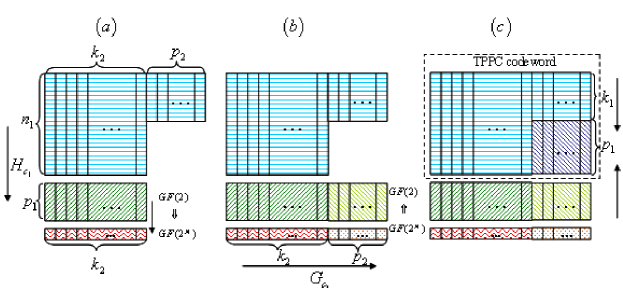
Figure 2: TPPC encoder of $C_{1}(n_{1},k_{1},p_{1})\otimes C_{2}(n_{2},k_{2},p_{2})$:(a) signatures calculated under $H_{c_{1}}$, then the $p_{1}$-bit signatures are mapped to $GF(2^{p_{1}})$ symbols, (b) $k_{2}$ signatures encoded by generator matrix $G_{c_{2}}$ into a $C_{2}$ codeword, then parity symbols are mapped back to $GF(2)$, (c) $p_{1}\times p_{2}$ TPPC parity bits are calculated by back substitution.

II-B2 Encoding of Tensor Product Parity Codes

The encoding of a TPPC can be performed using its binary parity check matrix, but the corresponding binary generator matrix is not guaranteed to possess algebraic properties that enable linear time encodability. Thus, an implementation-friendly approach would be to utilize the encoders of the constituent codes, which can be chosen to be linear time encodable.

Consider a binary code $C_{1}:(n_{1},k_{1},p_{1})$ that is the null space of parity check matrix $H_{c_{1}}$, and a non-binary code $C_{2}:(n_{2},k_{2},p_{2})$ defined on $GF(2^{p_{1}})$, the tensor-product concatenation is a binary $C_{3}:(n_{3},k_{3},p_{3})$, where:

$$n_{3}=n_{2}\times n_{1},k_{3}=n_{1}\times n_{2}-p_{1}\times p_{2},p_{3}=p_{1}\times p_{2}$$

Assume that $C_{1}$ is a cyclic code, and $C_{2}$ is any of the linear time encodable codes, where we choose a quasi-cyclic (QC) component code for the purpose of this study. Then, the encoders of $C_{1}$ and $C_{2}$ communicate via the following algorithm to generate a codeword of $C_{3}$, see Fig. 2:

1. Receive a block of $n_{1}\times k_{2}+k_{1}\times n_{2}-k_{1}\times k_{2}$ bits from the data source, call it major block $\alpha$.

2. Divide major block $\alpha$ into minor block $\beta$ of $n_{1}\times k_{2}$ bits, and minor block $\gamma$ of $k_{1}\times n_{2}-k_{1}\times k_{2}$ bits (i.e. $k_{1}\times p_{2}$ bits).

3. Divide block $\beta$ into $k_{2}$ columns each of $n_{1}$ bits. Then, for each column, calculate the intermediate $p_{1}$-bit signature under the parity check matrix of $C_{1}$. Using a feedback shift register (FSR) to calculate the signatures, the computational cost is $\propto n_{1}$ operations per signature, and $\propto n_{1}\times k_{2}$ for this entire step.

4. Convert intermediate signatures from $p_{1}$-bit strings into $GF(2^{p_{1}})$ symbols.

5. Encode the $k_{2}$ non-binary signatures into a $C_{2}$ codeword of length $n_{2}$. Using FSRs to encode the quasi-cyclic $C_{2}$, the computational complexity of this step is $\propto n_{2}$.

6. Convert computed signatures back into $p_{1}$-bit strings.

7. Divide block $\gamma$ into $p_{2}$ columns each of $k_{1}$ bits. Add $p_{1}$ blanks in each column to be filled with the parity bits of $C_{3}$. Then, align each column with the $p_{2}$ signatures computed in the previous step, leaving $p_{1}$ blanks in each column.

8. Fill blanks in the previous step such that the signature of data plus parity blanks under $C_{1}$ equals the corresponding aligned signature from step (vi). The parity can be calculated using the systematic $H_{c_{1}}$ and the method of back substitution which requires a computational complexity $\propto n_{1}$ per column.

The total computational complexity of this encoding algorithm is $\propto n_{1}\times k_{2}+n_{2}+n_{1}\times p_{2}$, i.e. it is $\propto n_{1}\times n_{2}=n_{3}$, which is the TPPC codeword length. Thus, we have shown- with some constraints- that if $C_{1}$ and $C_{2}$ are linear time encodable, then $C_{3}=C_{1}\otimes C_{2}$ is linear time encodable.

III T-EPCC-RS Codes

To demonstrate the algebraic properties of TPPC codes, we present an example code suitable for recording applications with $1/2$ KB sector size. Consider two component codes:

• A binary cyclic $(18,10)$ EPCC of example 2 above with rate $0.556$, $8$ parity bits, and parity check matrix in $GF(2^{8})$:

  $$H_{epcc}={\begin{array}[]{*{20}c}[1&\alpha&{\alpha^{2}}&{\alpha^{3}}&{\alpha^{4}}&{\alpha^{5}}&\ldots\\ {\alpha^{6}}&{\alpha^{7}}&{\alpha^{133}}&{\alpha^{134}}&{\alpha^{96}}&{\alpha^{90}}&\ldots\\ {\alpha^{82}}&{\alpha^{236}}&{\alpha^{234}}&{\alpha^{217}}&{\alpha^{92}}&{\alpha^{93}}&]_{1\times 18}.\\ \end{array}}$$ (1)

• A $(255,195)$ RS over $GF(2^{8})$, of rate $0.765$, $t=30$, and $60$ parity symbols.

The resulting TPPC is a binary $(4590,4110)$ code, of rate $0.896$, and redundancy of $480$ parity bits. For this code, a codeword is made of $255$ $18$-bit tensor symbols, of which, any combination of $30$ or less tensor symbol errors are correctable, provided that each $18$-bit tensor symbol has a single or multiple occurrence of a dominant error that is correctable by EPCC, those being combinations of error polynomials up to degree $9$. Furthermore, although the EPCC constituent code has a very low rate of $0.556$, the resulting T-EPCC has a high rate of $0.895$. Notably, in the view of the $18$-bit EPCC, this $61\%$ reduction in recorded redundancy corresponds to an SNR improvement of $2$ dB in a channel with rate penalty $\sim 10\log_{10}(1/R)$, and $4.1$ dB in a channel with rate penalty $\sim 10\log_{10}(1/R^{2})$.

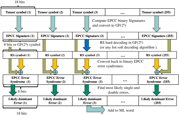
Figure 3: Hard decoder of $(18,10,8)$ EPCC $\otimes$ $(255,195,2t)$ RS of $t=30$ over $GF(2^{8})$.

III-A Hard Decoding of T-EPCC-RS Codes

Hard decoding of T-EPCC-RS directly reflects the code’s algebraic properties, and thus, serves to further clarify the concept of tensor product codes. Hence, we discuss the hard decoding approach before going into the design of soft decoding of T-EPCC codes. The decoding algorithm is summarized by the following procedure, see Fig. 3:

1. After hard slicing the output of the Viterbi channel detector, the signature of each tensor symbol is calculated under $H_{epcc}$. Each signature is then mapped into a Galois field symbol, where the sequence of non-binary signatures constitute an RS codeword - that is if the channel detector did not suffer any errors.

2. Any hard-input RS decoder, such as the Berlekamp-Massey decoder, acts to find a legitimate RS codeword based on the observed signature-sequence.

3. If the number of signature-symbols in error is larger than the RS correction power, RS decoding fails and the tensor product decoder halts.

4. Otherwise, if RS decoding is deemed successful, the corrected signature-symbol sequence is added to the original observed signature-symbol sequence to generate the “error syndrome-symbol” sequence.

5. Each error syndrome-symbol is mapped into an EPCC bit-syndrome of the corresponding tensor symbol.

6. Finally, EPCC decodes each tensor symbol to satisfy the error-syndrome generated by the component RS, in which it faces two scenarios:

   • A zero “error-syndrome” at the output of RS decoding indicates either no error occurred or a multiple error occurrence that has a zero EPCC-syndrome, which goes undetected. In this case, the EPCC decoder is turned off to save power.

   • A non zero “error-syndrome” will turn EPCC correction on. If the error-syndrome indicates a single error occurrence in the target set, then, the EPCC single error algebraic decoder is turned on. On the other hand, if the error-syndrome is not recognized, then EPCC list decoding is turned on with a reasonable-size list of test words.

   Note that although the number of EPCC codewords (tensor symbols) is huge, the decoder complexity is reasonable since EPCC decoding is turned on only for nonzero error-syndromes.

IV T-EPCC-$q$LDPC Codes

We learned from the design of T-EPCC-RS that the component signature-correcting codeword length can be substantially shorter than the competing single level code. Although the minimum distance is bound to be hurt if the increased redundancy does not compensate for the shorter codeword length, employing iterative soft decoding of the component signature-correcting code can recover performance if designed properly. While LDPC codes have strictly lower minimum distances compared to comparable rate and code length RS codes, the sparsity of its parity check matrix allows for effective belief propagation (BP) decoding. BP decoding of LDPC codes consistently performs better than the best known soft decoding algorithm for RS codes. Since the TPPC expansion enables the use of $2$ to $4$ times shorter component LDPC compared to a competing single level LDPC, a class of LDPC codes efficient at such short lengths are critical. LDPC codes on high order fields represent such good candidates. In that respect, [29] showed that the performance of binary LDPC codes in AWGN can be significantly enhanced by a move to fields of higher orders (extensions of $GF(2)$ being an example). Moreover, [29] established that for a monotonic improvement in waterfall performance with field order, the parity check matrix for very short blocks has to be very sparse. Specifically, column weight $3$ codes over $GF(q)$ exhibit worse bit-error-rate (BER) as $q$ increases, whereas column weight $2$ codes over $GF(q)$ exhibit monotonically lower BER as $q$ increases. These results were later confirmed in [30], where they also showed through a density evolution study of large $q$ codes that optimum degree sequences favor a regular graph of degree $2$ in all symbol nodes. On the other hand, for satisfactory error floor performance, we found that using a column weight higher than $2$ was necessary. This becomes more important as the minimum distance decreases for lower $q$. For instance, we found that a column weight of $3$ improved the error floor behavior of $GF(2^{6})$-LDPC at the expense of performance degradation in the waterfall region.

IV-A Design and Construction of $q$LDPC

The low rate and relatively low column weight design of $q$LDPC in a TPPC results in a very sparse parity check matrix, allowing the usage of high girth component $q$LDPC codes. To optimize the girth for a given rate, we employ the progressive edge growth (PEG) algorithm [30] in $q$LDPC code design. PEG optimizes the placement of a new edge connecting a particular symbol node to a check node on the Tanner graph, such that the largest possible local girth is achieved. Furthermore, PEG construction is very flexible, allowing arbitrary code rates, Galois field sizes, and column weights. In addition, modified PEG-construction with linear-time encoding can be achieved without noticeable performance degradation, facilitating the design of linear time encodable tensor product codes. Of the two approaches to achieve linear time encodability, namely, the upper triangular parity check matrix construction [30] and PEG construction with a QC constraint [31], we choose the latter approach, for which the designed codes have better error floor behavior. T-EPCC-$q$LDPC lends itself to iterative soft decoding quite naturally. Next, we present a low complexity soft decoder utilizing this important feature.

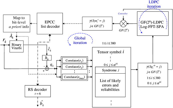
Figure 4: T-EPCC-$q$LDPC soft decoder of $(12,6,6)$ EPCC $\otimes$ $(380,\ 323)$ $GF(2^{6})$-LDPC.

IV-B Soft Decoding of T-EPCC-$q$LDPC

To fully utilize the power of the component codes in T-EPCC-$q$LDPC, we need to develop a soft iterative version of the hard decoder of T-EPCC-RS. To limit the complexity of the proposed soft decoder, sub-optimal detection post-processing is adopted instead of the maximum a posteriori (MAP) detector to evaluate tensor symbol signature reliabilities. The complexity of the optimal MAP detector matched to both the channel of memory length $L$ and $H_{epcc}$ of row length $p$ is exponential in $p+L-1$. We present a practical soft detection scheme that separates soft channel detection from tensor symbol signature detection, though, through a component signature-correcting LDPC in a TPPC setup, approaches the joint MAP performance through channel iterations. The main stages of the decoder are, see Fig. 4:

1. Detection postprocessing:

   • Utilizing a priori information from the previous decoding iteration, binary Viterbi generates the hard ML word based on channel observations, for which the error sequence is calculated and passed to the correlator bank.

   • A bank of local correlators estimates the probability of dominant error type/location pairs for all positions inside each tensor symbol.

2. Signature p.m.f. calculation:

   • For each tensor symbol, the list of most likely error patterns is constructed. This list includes single occurrences and a predetermined set of their combinations. The list is then divided into sublists, each under the signature value it satisfies.

   • For each tensor symbol, using each signature value’s error likelihood list, we find the signature p.m.f. of that symbol.

3. $q$-ary LDPC decoding:

   • Using the observed sequence of signature p.m.f.’s, we decode the component $q$-ary LDPC via FFT-based SPA.

   • For each tensor symbol, the LDPC-corrected signature p.m.f. is convolved with the observed signature p.m.f. at its input to generate the error-syndrome p.m.f..

4. EPCC decoding:

   • For each tensor symbol, we find the list of most probable error-syndromes and generate a list of test error words to satisfy each syndrome in the list.

   • A bank of parallel EPCC single-error correcting decoders generates a list of most probable codewords along with their reliabilities.

5. Bit-LLR feedback:

   • Using the codeword reliabilities we generate bit-level reliabilities that are fed back to the Viterbi detector and the detection postprocessing stage. Those bit-level reliabilities, serving as a priori information, favor paths which satisfy both the ISI and parity constraints.

We explain each of these steps in the following sections, but we replace any occurrence in the text of syndrome (signature) p.m.f. by syndrome (signature) multi-level log-likelihood ratios (mlLLR), as decoding will be entirely in the log domain for reasons explained below.

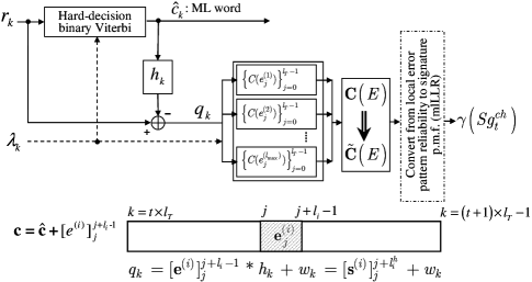
Figure 5: Bank of parallel error-matched correlators to find error pattern type/position reliabilities.

IV-B1 Detection Postprocessing

At this decoder stage we prepare a reliability matrix ${\bf{C}}\left(E\right)$ for error type/position pairs - captured in a tensor symbol of length $l_{T}$- that is usable by the next stage to calculate the tensor symbol’s signature mlLLR:

$$\begin{array}[]{*{21}c}{\bf{C}}\left(E\right)=&&&&&&&&&&&&&&&&&&&&\end{array}$$ (3)

$$\begin{array}[]{*{20}c}{}\hfil&\begin{array}[]{*{20}c}0&&&&1&&&&\cdots&&&l_{T}\\ \end{array}\\ \begin{array}[]{*{20}c}1\\ 2\\ \vdots\\ l_{max}\\ \end{array}&\left[{\begin{array}[]{*{20}c}{C(e_{0}^{(1)})}&{C(e_{1}^{(1)})}&\cdots&{C(e_{l_{T}-1}^{(1)})}\\ {C(e_{0}^{(2)})}&{C(e_{1}^{(2)})}&\cdots&{C(e_{l_{T}-1}^{(2)})}\\ \vdots&\vdots&\ddots&\vdots\\ {C(e_{0}^{(l_{max})})}&{C(e_{1}^{(l_{max})})}&\cdots&{C(e_{l_{T}-1}^{(l_{max})})}\\ \end{array}}\right]\par\\ \end{array}$$ (15)

where $C(e_{k}^{(i)})$ is the error pattern (type $i$/ position $k$) reliability measure computed by the maximum a posteriori (MAP)-based error-pattern correlator shown in Fig. 5. The bank of local correlators discussed here was also employed in [18] for AWGN channels, and in [19] for data-dependent noise environments. We now discuss how to generate these local metrics. Let $r_{k}$ be the channel detector input sequence $r_{k}={c}_{k}*h_{k}+w_{k}$, where ${c}_{k}$ is the bipolar representation of the recorded codeword sequence, $h_{k}$ is the partial response channel of length $l_{h}$, and $w_{k}$ is zero-mean AWGN noise with variance $\sigma^{2}$. Also, let ${q}_{k}=r_{k}-(\hat{c}_{k}*h_{k})=(c_{k}-\hat{c}_{k})*h_{k}+w_{k}$ be the channel detector’s output error sequence. If a target error pattern sequence $e_{k}^{(i)}$ occurs at positions from $k=j$ to $k=j+l_{i}-1$, then $q_{k}$ can be written as

$$\begin{split}q_{k}&=[\textbf{c}-\hat{\textbf{c}}^{(i)}]_{j}^{j+l_{i}-1}*h_{k}+w_{k}\\ &=[\textbf{e}^{(i)}]_{j}^{j+l_{i}-1}*h_{k}+w_{k}\\ &=[\textbf{s}^{(i)}]_{j}^{j+l_{i}^{h}}+w_{k}\end{split}$$ (16)

where $s_{k}^{(i)}$ is the channel response of the error sequence, and is given by $s_{k}^{(i)}=e_{k}^{(i)}*h_{k}$, and $l_{i}^{h}=l_{i}+l_{h}-2$. Note that we define the start of the tensor symbol at $j=0$. So, if $j<0$, then the error pattern starting position is in a preceding tensor symbol.

The reliability for each error pattern with starting position, $j$, can be computed by the local a posteriori probabilities (ignoring tensor symbol boundaries for now):

$$\Pr\left({\left.{[\textbf{e}^{(i)}]_{j}^{j+l_{i}-1}}\right|[\textbf{r}]_{j}^{j+l_{i}^{h}},[{\bf{\hat{c}}}]_{j-l_{h}+1}^{j+l_{i}^{h}}}\right)$$

$$=\Pr\left({\left.{[\textbf{s}^{(i)}]_{j}^{j+l_{i}^{h}}}\right|[\textbf{q}]_{j}^{j+l_{i}^{h}},[{\bf{\hat{c}}}]_{j-l_{h}+1}^{j+l_{i}^{h}}}\right).$$ (17)

The most likely assumed error type/position pair in a tensor symbol maximizes the a posteriori probability ratio of its reliability to the reliability of the most probable error event (the competing event in this case would be the ML word itself, with no error occurrence assumed at the output of Viterbi detection). Hence, utilizing (IV-B1) and Bayes rule, the ratio to maximize becomes

$$\displaystyle\begin{array}[]{*{1}l}\displaystyle\frac{{\Pr\left({\left.{\textbf{e}_{j}^{(i)}}\right|{\bf{\hat{c}}},[\textbf{q}]_{j}^{j+l_{i}^{h}}}\right)}}{{\Pr\left({\left.{\left[{{\rm{\textbf{ML word}}}}\right]_{j}^{j+l_{i}-1}}\right|{\bf{\hat{c}}},[\textbf{q}]_{j}^{j+l_{i}^{h}}}\right)}}=\\ \displaystyle\frac{{\Pr\left({\left.{[{\bf{q}}]_{j}^{j+l_{i}^{h}}}\right|[{\bf{\hat{c}}}]_{j-l_{h}+1}^{j+l_{i}^{h}},[{\bf{s}}^{(i)}]_{j}^{j+l_{i}^{h}}}\right)\Pr\left({[{\bf{s}}^{(i)}]_{j}^{j+l_{i}^{h}}}\right)}}{{\Pr\left({\left.{[{\bf{q}}]_{j}^{j+l_{i}^{h}}}\right|[{\bf{\hat{c}}}]_{j-l_{h}+1}^{j+l_{i}^{h}},[{\bf{\tilde{s}}}^{(i)}]_{j}^{j+l_{i}^{h}}}\right)\Pr\left({[{\bf{\tilde{s}}}^{(i)}]_{j}^{j+l_{i}^{h}}}\right)}}\end{array}$$ (20)

where $[{\bf{\tilde{s}}}^{(i)}]_{j}^{j+l_{i}^{h}}$ is the ML word’s noiseless channel response. Given the noise model, $[{\bf{q}}]_{j}^{j+l_{i}^{h}}$ is a sequence of independent Gaussian random variables with variance $\sigma^{2}$. Therefore, maximizing (20) can be shown to be equivalent to maximizing the log-likelihood local measure [18]:

$$C(e_{j}^{(i)})=\sum\limits_{k=j}^{j+l_{i}^{h}}\frac{1}{{2\sigma^{2}}}\left({q_{k}^{2}-(q_{k}-s_{k}^{(i)})^{2}}\right)-\log\frac{{\Pr([{\bf{\tilde{s}}}^{(i)}]_{j}^{j+l_{i}^{h}})}}{{\Pr([{\bf{s}}^{(i)}]_{j}^{j+l_{i}^{h}})}}$$ (21)

where the a priori bias in (21) is evaluated as:

$$\log\frac{{\Pr([{\bf{\tilde{s}}}^{(i)}]_{j}^{j+l_{i}^{h}})}}{{\Pr([{\bf{s}}^{(i)}]_{j}^{j+l_{i}^{h}})}}=\sum\limits_{k=j,\hat{c}_{k}=+1}^{j+l_{i}^{h}}{\lambda_{k}}-\sum\limits_{k=j,\hat{c}_{k}=-1}^{j+l_{i}^{h}}{\lambda_{k}}$$ (22)

where $\lambda_{k}$ is the a priori LLR of the error-event bit at position $k$ as received from the outer soft decoder, and we are assuming here that error event sequences do not include $0$ bits, i.e., the ML sequence and error sequence do not agree for the entire duration of the error event. Equation (21) represents the “local” error-pattern correlator output in the sense that it essentially describes the correlator operation between $q_{k}$ and the channel output version of the dominant error pattern $e_{j}^{(i)}$ within the local region $[j,j+l_{i}^{h}]$. However, equation (21) ignores that errors can span tensor symbol boundaries when $j<0$ or $j+l_{i}-1>l_{T}-1$. For instance, an error in the first bit of the tensor symbol can result from a single error event in that bit, a double error event in the last bit of the preceding tensor symbol, a triple error event occurring two bits into the previous symbol, and so on. Hence, the probability of an error in the first bit is the sum of all these parent error event probabilities. Moreover, this can be easily generalized to boundary errors extending beyond the first bit. In a similar manner, an error in the last bit of a tensor symbol can result from a single error event in that bit, a double error event starting in that bit and continuing into the next tensor symbol, a triple error starting at the last bit and continuing into the next tensor symbol, and so on. Again, the probability of an error event in that bit is the sum of the probabilities of all these parent events. Moreover, we have to nullify the probability of the parent error events in the modified reliability matrix since they are already accounted for in the last bit’s reliability calculation. Furthermore, this can also be generalized to error events starting earlier than the last bit and extending into the next tensor symbol. In summary, to calculate a modified metric relevant to the current tensor symbol, we utilize the following procedure:

• $\forall i$ at $j=0$, modify $C(e_{0}^{(i)})$

  $$\tilde{C}(e_{0}^{(i)})=\mathop{max^{*}}\limits_{k=i}^{l_{max}}\left({C(e_{-k+i}^{(k)})}\right),$$

  independently for each $i$, where $l_{max}$ is the maximum length of a targeted error pattern.

• Starting at $i=1$ and $j=l_{T}-1$, do:

  1. $\tilde{C}(e_{j}^{(i)})=\mathop{max^{*}}\limits_{k=i}^{l_{max}}\left({C(e_{j}^{(k)})}\right)$.

  2. $\forall k>i$, set $\tilde{C}(e_{j}^{(k)})=-\infty$.

  3. Set $i=i+1$, $j=j-1$.

  4. If $i<l_{max}$ go back to (i).

We assume here that dominant error events span only two tensor symbols at a time and that they do not include error free gaps, which is certainly true for the case study of this paper. Following this procedure we obtain the modified reliability matrix ${\bf{\tilde{C}}}\left(E\right)$.

IV-B2 Signature mlLLR Calculation

For each tensor symbol $i$, utilizing ${\bf{\tilde{C}}}\left(E\right)$, we need to find the p.m.f. or the log domain mlLLR of its signature $Sg_{i}\in GF(2^{p_{epcc}})$, for EPCC with $p_{epcc}$ parity bits. To limit the computational complexity of this calculation, we construct a signature only from the dominant errors and a subset of their multiple occurrences. Denote $\hat{Pr}(Sg_{i}=\alpha^{j-1})$ as the running estimate of the p.m.f. at $\alpha^{j-1}$, and $\hat{\gamma}(Sg_{i}=\alpha^{j-1})=\log(\hat{Pr}(Sg_{i}=\alpha^{j-1}))$ as the running estimate of mlLLR. Denote a one dimensional index of ${\bf{\tilde{C}}}\left(E\right)$ as $p^{rc}=(p_{c}\times l_{max})+p_{r}$ corresponding to the $p_{r}$-th row and $p_{c}$-th column of ${\bf{\tilde{C}}}\left(E\right)$ and error $E(p^{rc})$. We choose the dominant list as the $L$ patterns with the largest corresponding elements of ${\bf{\tilde{C}}}\left(E\right)$ having indexes $\{p_{i}^{rc}\}^{i=L}_{i=1}$. Based on this list, we developed the following procedure to compute $\hat{\gamma}(Sg_{i}=\alpha^{j-1})$:

• Step $1$ (Single occurrences):

  $$\begin{array}[]{*{10}c}\hat{\gamma}(Sg_{i}=\alpha^{j-1})=\mathop{max^{*}}\limits_{k=p_{1}^{rc}}^{p_{L}^{rc}}\left({\tilde{C}\left(k\right)}\right),&&&&&&\end{array}$$ (24)

  $$\forall k:\mathop{G_{f}}\limits_{q_{epcc}}(H_{epcc}\times[\hat{c}_{i\times l_{T}}^{(i+1)\times l_{T}-1}\oplus E(k)]^{t})=\alpha^{j-1}$$

  where $q_{epcc}=2^{p_{epcc}}$, and $G_{f}(.)$ is an operator that maps $p_{epcc}$-bit vectors into $GF(q_{epcc})$ symbols.

• Step $2$ (Double occurrences):

  $$\begin{array}[]{*{13}c}\hat{\gamma}(Sg_{i}=\alpha^{j-1})=&&&&&&&&&&&&\end{array}$$ (27)

  $$max^{*}\left(\begin{array}[]{*{1}c}\hat{\gamma}\left(Sg_{i}=\alpha^{j-1}\right)\\ \left\{{\tilde{C}\left(k\right)+\tilde{C}\left(m\right)}\right\}_{k=p_{1}^{rc},m=p_{1}^{rc}}^{p_{L}^{rc},p_{L}^{rc}}\end{array}\right),$$ (30)

  $$\forall\{k,m\}:\mathop{\mathbb{missing}}{D}\limits_{k\neq m}(E(k),E(m))>E_{free},$$

  $$\mathop{G_{f}}\limits_{q_{epcc}}(H_{epcc}\times[\hat{c}_{i\times l_{T}}^{(i+1)\times l_{T}-1}\oplus E(k)\oplus E(m)]^{t})=\alpha^{j-1}$$

  where $\mathbb{D}$ is the error free distance between the two errors, $E_{free}=l_{h}-1$ is the error free distance of the channel beyond which the errors are independent.

• …

• Step $M$ ($M$ occurrences):

  $$\begin{array}[]{*{13}c}\hat{\gamma}(Sg_{i}=\alpha^{j-1})=&&&&&&&&&&&&\end{array}$$ (33)

  $$max^{*}\left(\begin{array}[]{*{1}c}\hat{\gamma}\left(Sg_{i}=\alpha^{j-1}\right)\\ \left\{{\sum_{\xi=1}^{M}\tilde{C}\left(q_{\xi}\right)}\right\}_{q_{\xi}=p_{1}^{rc},\xi=1,...,M}^{p_{L}^{rc}}\end{array}\right),$$ (36)

  $$\forall\{q_{1},q_{2},...,q_{M}\}:\mathop{\mathbb{missing}}{D}\limits_{s,t,s\neq t}(E(q_{s}),E(q_{t}))>E_{free},$$

  $$\mathop{G_{f}}\limits_{q_{epcc}}(H_{epcc}\times[\mathop{\bigoplus}\limits_{\xi=1}^{\xi=M}E(q_{\xi})\oplus\hat{c}_{i\times l_{T}}^{(i+1)\times l_{T}-1}]^{t})=\alpha^{j-1}$$

• Step $M+1$ (ML-signature reliability; computed so that the resulting signature p.m.f. sums to $1$):

  $$\begin{array}[]{*{16}l}\breve{\gamma}\left(Sg_{i}=\alpha^{\beta_{ML}}\right)=&&&&&&&&&&&&\end{array}$$ (39)

  $$-max^{*}\left(\begin{array}[]{*{1}c}0\\ \mathop{max^{*}}\limits_{j=-\infty,j\neq\beta_{ML}+1}^{q_{epcc}-1}\hat{\gamma}\left(Sg_{i}=\alpha^{j-1}\right)\end{array}\right)$$ (42)

  $$\hat{\gamma}\left(Sg_{i}=\alpha^{\beta_{ML}}\right)=max^{*}\left(\begin{array}[]{*{1}c}\breve{\gamma}\left(Sg_{i}=\alpha^{\beta_{ML}}\right)\\ \hat{\gamma}\left(Sg_{i}=\alpha^{\beta_{ML}}\right)\end{array}\right)$$ (45)

  $$\hat{\gamma}(Sg_{i}=\alpha^{j-1})=\hat{\gamma}(Sg_{i}=\alpha^{j-1})+\hat{\gamma}(Sg_{i}=\alpha^{\beta_{ML}}),$$

  $$j=-\infty,1,...,q_{epcc}-1;j\neq\beta_{ML}+1.$$

• Step $M+2$ (Normalization):

  $$\gamma(Sg_{i}=\alpha^{j-1})=\hat{\gamma}(Sg_{i}=\alpha^{j-1})-\hat{\gamma}(Sg_{i}=\alpha^{-\infty}).$$ (47)

In steps $1$ through $M$, to calculate the log-likelihood of signature $i$ assuming value $\alpha^{j-1}$, we sum the probabilities of all presumed single and multiple errors in the ML word whose signatures equal $\alpha^{j-1}$. This is equivalent to performing the $max^{*}$ operation in the log domain on error reliabilities dictated by ${\bf{\tilde{C}}}\left(E\right)$. However, to limit the complexity of this stage, we only use a truncated set of possible error combinations, in all steps from $1$ to $M$. Also, for signature values that do not correspond to any of the combinations, we set their reliability to $-\infty$, or more precisely, a reasonably large negative value in practical decoder implementation. Since there are many such signature values, the corresponding constructed p.m.f. will be sparse.

In step $M+1$, the likelihood of the ML signature value is computed so that the p.m.f. of the tensor symbol signature sums to $1$. In this step, the $max^{*}$ operation in (45) is a reflection of the fact that in previous steps, $1$ through $M$, some multiple error occurrences have the same signature as the ML tensor symbol value. So, we have to account for such error instances in the running estimate of the ML signature reliability. These events correspond to cases where error events are not detectable by $H_{epcc}$, i.e., they belong to the null space of $H_{epcc}$. In step $M+2$, the mlLLR of the tensor symbol is centered around $\hat{\gamma}(Sg_{i}=0)$ to prevent the $q$LDPC SPA messages from saturating after a few BP iterations.

IV-B3 $q$-ary LDPC Decoding

Now, the sequence of signature mlLLRs is passed as multi-level channel observations to the $q$LDPC decoder. We choose to implement the log-domain $q$-ary fast Fourier transform-based SPA (FFT-SPA) decoder in [35] for this purpose. The choice of log-domain decoding is essential, since if we use the signature p.m.f. as input, the SPA would run into numerical instability resulting from the sparse p.m.f. generated by the preceding stage.

The LDPC output posteriori mlLLRs correspond to the signatures of tensor symbols, rather than the syndromes of errors expected by EPCC decoding. Similar to the decoder of T-EPCC-RS, error-syndrome $Syn_{i}^{e}$ is the finite field sum of the LDPC’s input channel observation of signature $i$, $Sg_{i}^{ch}$, and output posteriori signature reliability, $Sg_{i}^{p}$. Moreover, the addition of hard signatures corresponds to the convolution of their p.m.f.’s, and this convolution in probability domain corresponds to the following operation in log-domain:

$$\begin{array}[]{*{13}c}\hat{\gamma}(Syn_{i}^{e}=\alpha^{\beta_{e}})=&&&&&&&&&&&&\end{array}$$ (49)

$${max^{*}}\left(\begin{array}[]{*{1}c}\hat{\gamma}(Syn_{i}^{e}=\alpha^{\beta_{e}})\\ \gamma(Sg_{i}^{ch}=\alpha^{\beta_{ch}})+\gamma(Sg_{i}^{p}=\alpha^{\beta_{p}})\end{array}\right),$$ (52)

$$\forall\{\beta_{ch},\beta_{p}\}:\alpha^{\beta_{e}}=\alpha^{\beta_{ch}}\mathop{\oplus}\limits_{GF(q_{epcc})}\alpha^{\beta_{p}},$$

$$\beta_{ch}=-\infty,0,...,q_{epcc}-2;$$

$$\beta_{p}=-\infty,0,...,q_{epcc}-2.$$

The error-syndrome mlLLR is later normalized, similar to LDPC BP mlLLR message normalization, according to:

$$\gamma(Syn_{i}^{e}=\alpha^{\beta_{e}})=\hat{\gamma}(Syn_{i}^{e}=\alpha^{\beta_{e}})-\hat{\gamma}(Syn_{i}^{e}=\alpha^{-\infty}),$$

$$\forall\beta_{e}=-\infty,0,...,q_{epcc}-2.$$ (54)

IV-B4 EPCC Decoding

An error-syndrome will decode to many possible error events due to the low minimum distance of single-error correcting EPCC. However, EPCC relies on local channel side information to implement a list-decoding-like procedure that enhances its multiple error correction capability. Moreover, the short codeword length of EPCC reduces the probability of such multiple error occurrences considerably. To minimize power consumption, EPCC is turned on for a tensor symbol $i$ only if the most likely value of the error-syndrome mlLLR is nonzero, i.e., $\mathop{\arg\max}\limits_{\alpha^{\beta}\in GF(q_{epcc})}\gamma(Syn_{i}^{e}=\alpha^{\beta})\neq\alpha^{-\infty}$, indicating that a resolvable error has occurred. After this, a few syndrome values, $3$ in our case, most likely according to the mlLLR, are decoded in parallel. For each of these syndromes, the list decoding algorithm goes as [18, 19]:

• A test error word list is generated by inserting the most probable combination of local error patterns into the ML tensor symbol.

• An array of parallel EPCC single-pattern correcting decoders decodes the test words to produce a list of valid codewords that satisfy the current error-syndrome.

• The probability of a candidate codeword is computed as the sum of likelihoods of its parent test-word and the error pattern separating the two.

• Each candidate codeword probability is biased by the likelihood of the error-syndrome it is supposed to satisfy.

In addition, when generating test words, we only combine independent error patterns that are separated by the error free distance of the ISI channel.

IV-B5 Soft Bit-level Feedback LLR Calculation

The list of candidate codewords and probabilities are used to generate bit level-probabilities in a similar manner to  [27, 19]. The conversion of word-level reliability into bit-level reliability for a given bit position can be done by grouping the candidate codewords into two groups, according to the binary value of the hard decision bit in that bit position, and then performing group-wise summing of the word-level probabilities. Three scenarios are possible for this calculation:

1. The candidate codewords do not all agree on the bit decision for location $k$; then, given the list of codewords and their accompanying a posteriori probabilities, the reliability $\lambda_{k}$ of the coded bit $c_{k}$ is evaluated as

   $$\lambda_{k}=\log\frac{\sum_{\mathbf{c}\in\textbf{S}_{k}^{+}}Pr(\mathbf{c}|\mathbf{\hat{c}},\mathbf{r})}{\sum_{\mathbf{c}\in\textbf{S}_{k}^{-}}Pr(\mathbf{c}|\mathbf{\hat{c}},\mathbf{r})}$$ (55)

   where $\textbf{S}_{k}^{+}$ is the set of candidate codewords where $c_{k}=+1$, and $\textbf{S}_{k}^{-}$ is the set of candidate codewords where $c_{k}=-1$

2. Although rare for such short codeword lengths, in the event that all codewords do agree on the decision for $c_{k}$, a method inspired by [27] is adopted for generating soft information as follows

   $$\lambda_{k}=\beta^{iter}\times\lambda_{max}\times\hat{d}_{k}$$ (56)

   where $\hat{d}_{k}$ is the bipolar representation of the agreed-upon decision, $\lambda_{max}$ is a preset value for the maximum reliability at convergence of turbo performance, and the multiplier $\beta^{iter}<1$ is a scaling factor. $\beta^{iter}\ll 1$ in the first global iterations and is increased to $1$ as more global iterations are performed and the confidence in bit decisions improved. Thus, this back-off control process reduces the risk of error propagation.

3. The heuristic scaling in (56) is again useful when EPCC is turned off for a tensor symbol, in case the most likely error-syndrome being $0$. Then, the base hard value of the tensor symbol corresponds to the most likely error event found as a side product in stage $2$ of the T-EPCC-$q$LDPC decoder.

IV-C Stopping Criterion for T-EPCC-$q$LDPC and RS Erasure Decoding

Due to the ambiguity in mapping tensor symbols to signatures and syndromes to errors in stages $2$ and $4$ of the decoder, respectively, the possibility of non-targeted error patterns, or errors that have zero error-syndromes that are transparent to $H_{epcc}$, a second line of defense is essential to take care of undetected errors. Therefore, an outer RS code of small correction power $t_{out}$ is concatenated to T-EPCC-$q$LDPC to take care of the imperfections of the component EPCC. Several concurrent functions are offered by this code, including:

• Stopping Flag: If the RS syndrome is zero, then, global iterations are halted and decisions are released.

• Outer ECC: Attempt to correct residual errors at the output of EPCC after each global iteration.

• Erasure Decoding: If the RS syndrome is nonzero, then, for those tensor symbols that EPCC was turned on, declare their bits as erasures. Next, find the corresponding RS symbol erasures, and attempt RS erasure decoding which is capable of correcting up to $2\times t_{out}$ such erasures. In this case, T-EPCC acts as an error locating code.

V Simulation Results and Discussion

We compare three coding systems based on LDPC: conventional binary LDPC, $q$-ary LDPC, and T-EPCC-$q$LDPC, where all the component LDPC codes are regular and constructed by PEG with a QC constraint. We study their sector error rate (SER) performance on the ideal equalized partial response target $1+0.85D$ corrupted by AWGN, and with coding rate penalty $10\log_{10}(1/R)$. The nominal systems run at a coding rate of $0.9$. The minimum SNR required to achieve reliable recording at this rate is $3.9$ dB, estimated by following the same approach as in [28].

V-A Single-level BLDPC & $q$LDPC Simulation Results

In Fig. 6, we compare SER of the following LDPC codes, each constructed by PEG with a QC constraint:

• A $(4550,4095)$ $GF(2)$-LDPC, of column weight $5$, and circulant size $91$ bits. The channel detector is a $2$ state binary BCJR.

• A $(570,510)$ $GF(2^{8})$-LDPC, of codeword length $4560$ bits, column weight $2$, and circulant size of $15$ symbols. The channel detector is a symbol-BCJR with $256$ branches emanating from each of $2$ states.

• A $(760,684)$ $GF(2^{6})$-LDPC, of codeword length $4560$ bits, column weight $2$, and circulant size of $19$ symbols. The channel detector is a symbol-BCJR with $64$ branches emanating from each of $2$ states.

• A $(775,700)$ $GF(2^{6})$-LDPC, of codeword length $4650$ bits, column weight $3$, and circulant size of $25$ symbols. The channel detector is a symbol-BCJR with $64$ branches emanating from each of $2$ states.

For the binary LDPC turbo equalizer, we run a maximum of $10\times 50$ iterations, $10$ global, and $50$ LDPC BP iterations. For the $q$-ary turbo equalizers, on the other hand, we run a maximum of $3\times 50$ iterations. A column weight of $2$ gives the best waterfall performance of $q$-ary LDPC. However, $GF(2^{6})$-LDPC exhibits an error floor as early as at SER $6\times 10^{-4}$, whereas a higher order field of $GF(2^{8})$ does not show such a tendency down to $1\times 10^{-5}$. Nevertheless, the prohibitive complexity of $GF(2^{8})$ symbol-BCJR makes $GF(2^{6})$-LDPC a more attractive choice. Still, we need to sacrifice $GF(2^{6})$-LDPC’s waterfall performance gains to guarantee a lower error floor. For that purpose, we move to a column weight $3$ $GF(2^{6})$-LDPC that is $1.37$ dB away at $1\times 10^{-5}$ from the independent uniformly-distributed capacity $C_{I.U.D.}$ of the channel [28], and $0.37$ dB away from $GF(2^{8})$-LDPC a the same SER. In this simulation study, we have observed that while binary LDPC can gain up to $0.4$ dB through $10$ channel iterations before gain saturates, $GF(2^{8})$-LDPC and $GF(2^{6})$-LDPC achieve very little iterative gain by going back to the channel, between $0.09$ to $0.12$ dB through $3$ channel iterations. One way to explain this phenomenon, is that symbol-level LDPC decoding divides the bit stream into LDPC symbols that capture the error events introduced by the channel detector, rendering the binary inter-symbol interference limited channel into a memoryless multi-level AWGN limited channel. Nonetheless, error events spanning symbol boundaries reintroduce correlations between LDPC symbols that are broken only by going back to the channel. In other words, if it was not due to such boundary effects, a $q$-ary LDPC equalizer would not exhibit any iterative turbo gain whatsoever. Nonetheless, full-blown symbol BCJR is still too complex to justify salvaging the small iterative gain by performing extra channel iterations [33]. This is where error event matched decoding comes into the picture, which leads us to the results of the next section.

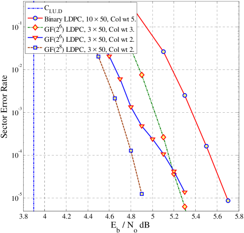
Figure 6: Comparing SER of: $10\times 50$ iterations of binary LDPC, $3\times 50$ iterations of $GF(2^{8})$-LDPC of column weight $2$, and $3\times 50$ iterations of $GF(2^{6})$-LDPC of column weights $2$ and $3$. Minimum SNR to achieve reliable recording at coding rate $0.9$ is $3.9$ dB for $1+0.85D$.

V-B T-EPCC-$q$LDPC Simulation Results

We first construct two T-EPCC-$q$LDPC codes of rate $0.9$, the same rate as the competing single-level $q$LDPC. These TPPC’s are based on EPCC $(12,6)$ of example 1. The codes constructed are:

• TPPC-A: A $1/2$ KB sector, binary $(4680,4212)$ TPPC, of rate $0.9$, and $468$ parity bits, based on a component $(390,312)$ PEG-optimized QC $GF(2^{6})$-LDPC, of rate $0.8$, column weight $3$, and circulant size $26$.

• TPPC-B: A $1$ KB sector, binary $(9360,8424)$ TPPC, of rate $0.9$, and $936$ parity bits, based on a component $(780,624)$ PEG-optimized QC $GF(2^{6})$-LDPC, of rate $0.8$, column weight $3$, and circulant size $52$.

First, we study the SER of T-EPCC-$q$LDPC just up to the component $GF(2^{6})$ LDPC decoder, and only at the first channel pass. This SER is function of the Viterbi symbol error rate, and the accuracy of generating signature mlLLRs, in addition to the component LDPC employed. This SER represents the best that the TPPC code can do, under the assumption of perfect component EPCC, i.e., as long as $q$LDPC generates a clean codeword of signature-symbols, then EPCC generates a clean codeword of data-symbols. Fig. 7 shows the ideal SER of these two TPPC codes, assuming perfect EPCC, compared to single-level $GF(2^{6})$-LDPC and $GF(2^{8})$-LDPC. Ideal $1/2$ KB TPPC has about the same SER as single level $GF(2^{6})$-LDPC at $3\times 10^{-5}$ SER. In $1/2$ KB TPPC, the component $GF(2^{6})$-LDPC has half the codeword length of the single level counterpart, saving $50\%$ of the decoder complexity, while delivering similar SER performance. The TPPC component $q$LDPC faces a harsher channel than single-level $q$LDPC, because the symbol error probability of $6$-bit data symbols is strictly less than the symbol error probability of $6$-bit signature symbols, where signature symbols are compressed down from $12$-bit data symbols. Also, the shorter codeword length of component $q$LDPC hurts its minimum distance. Still, these impairments are effectively compensated for by an $11.4\%$ increase in the redundancy of the TPPC component LDPC. On the other hand, if we match the codeword length of TPPC’s component LDPC to single-level LDPC, as part of constructing $1$ KB TPPC, then, $1$ KB TPPC will have similar decoder complexity to $1/2$ KB single-level LDPC with about $0.2$ dB SNR advantage for $1$ KB ideal TPPC at $3\times 10^{-5}$ SER.

Due to the imperfections of EPCC design, including mis-correction due to one-to-many syndrome to error position mapping, and undetected errors due to EPCC’s small minimum distance, achieving the ideal performance in Fig. 7 is not possible in one channel pass. In addition, an outer code is necessary to protect against undetected errors and provide a stopping flag for the iterative decoder. Hence, one can think of an implementation of the full T-EPCC-$GF(2^{6})$LDPC decoder that includes an outer $t=6$ $(421,409)$ RS for the $1/2$ KB case, and an outer $t=12$ $(842,818)$ RS for the $1$ KB case, so as to protect against EPCC residual errors. These outer RS codes are defined on $GF(2^{10})$ and have rate $0.972$. However, this concatenation setup will run at a lower code rate of $0.875$, which can incur an SNR degradation larger than $0.25$ dB for a noise environment characterized by the rate penalty $10\log_{10}(1/R^{\delta}),\ \delta\geq 2$. In a more thoughtful approach, one can preserve the nominal code rate of $0.9$ and redistribute the redundancy between the inner TPPC and outer RS to achieve an improved tradeoff between miscorrection probability and the inner TPPC’s component LDPC code strength. In that spirit, we construct the following concatenated codes:

• TPPC-C: A $1/2$ KB sector, binary $(4560,4218)$ TPPC, of rate $0.925$, and $342$ parity bits, based on a component $(380,323)$ PEG-optimized QC $GF(2^{6})$-LDPC, of rate $0.85$, column weight $3$, and circulant size $19$. An outer $t=6$ $(422,410)$ RS code of rate $0.972$ is included, resulting in a total system rate of $0.9$.

• TPPC-D: A $1$ KB sector, binary $(9120,8436)$ TPPC, of rate $0.925$, and $684$ parity bits, based on a component $(760,646)$ PEG-optimized QC $GF(2^{6})$-LDPC, of rate $0.85$, column weight $3$, and circulant size $38$. An outer $t=12$ $(844,820)$ RS code of rate $0.972$ is included, resulting in a total system rate of $0.9$.

The control mechanism of iterative decoding for these codes is as follows: if EPCC results in less than $6$ RS symbol errors for the $1/2$ KB design or less than $12$ for the $1$ KB design, or if EPCC generates more errors than this, but declares less than $12$ erasures for $1/2$ KB or $24$ erasures for $1$ KB, then, decoding halts and decisions are released. Otherwise, one more channel iteration is done by passing EPCC soft bit-level LLR’s to Viterbi detection and the bank of error-matched correlators.

Simulation results in Fig. 8, for a noise environment of rate penalty $10\log_{10}1/R$, demonstrate that after $3$ channel iterations, the ideal and practical performances of the new TPPC codes almost lock, while incurring minimal SNR degradation. Also, $1/2$ KB TPPC saves $50\%$ of decoder complexity while achieving the same SER performance as single level LDPC for an additional SNR cost of $0.04$ dB at SER $1\times 10^{-5}$. Hence, TPPC-C represents a tradeoff between the lower complexity of $GF(2)$-LDPC and performance advantage of $GF(2^{6})$-LDPC, whereas $1$ KB TPPC has the same decoding complexity as single-level LDPC while furnishing $0.18$ dB gain at $5\times 10^{-6}$ SER. In terms of channel detector implementation complexity, the complexity and latency of $GF(2^{6})$-BCJR in the single level code far exceeds the overall complexity of the non-LDPC parts of two level T-EPCC-$GF(2^{6})$LDPC including Viterbi detection. At the same time, signature mlLLR generation, EPCC decoding, and bit-LLR generation are all implemented tensor-symbol by tensor-symbol, achieving full parallelism on the tensor-symbol level. Furthermore, it is only when $q$LDPC finds a syndrome error that EPCC decoding is turned on for each tensor symbol. To eliminate redundant computations in the iterative decoder, branch metric computation in Viterbi and (21) is only required at the first pass. For all subsequent iterations, however, only the a priori bias is updated in the second term of (21), and the branch update of Viterbi [34].

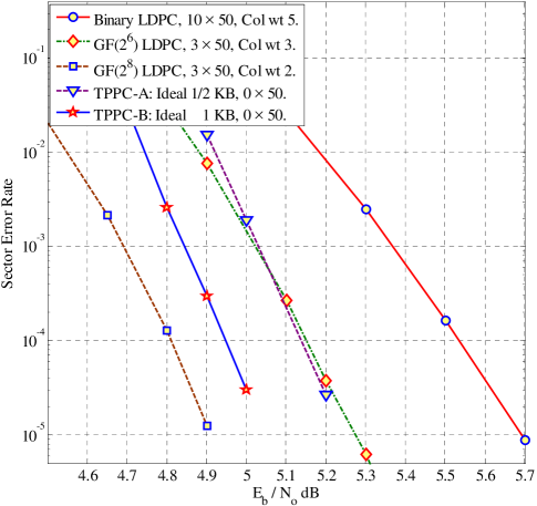
Figure 7: Comparing SER of: $10\times 50$ iterations of binary LDPC, $3\times 50$ iterations of $GF(2^{8})$-LDPC of column weight $2$, $3\times 50$ iterations of $GF(2^{6})$-LDPC of column weight $3$, and $0\times 50$ iterations of ideal $1/2$ KB and $1$ KB T-EPCC-$GF(2^{6})$LDPC based on column weight $3$ LDPC.

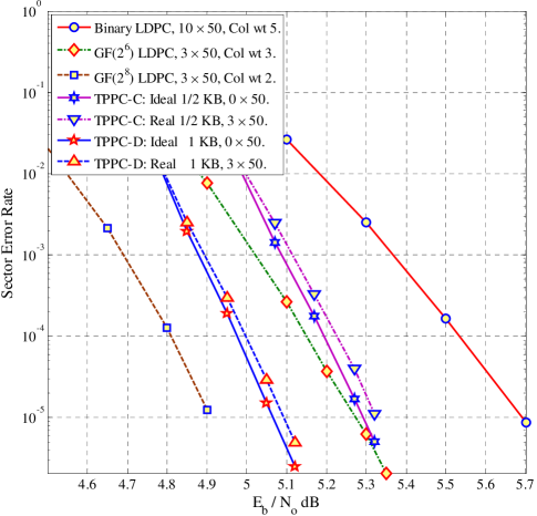
Figure 8: Comparing SER in environment of rate penalty$10\log_{10}1/R$: $10\times 50$ iterations of binary LDPC, $3\times 50$ iterations of $GF(2^{8})$-LDPC of column weight $2$, $3\times 50$ iterations of $GF(2^{6})$-LDPC of column weight $3$, and $3\times 50$ iterations of practical $1/2$ KB T-EPCC-$GF(2^{6})$LDPC+RS($t=6$), and $1$ KB T-EPCC-$GF(2^{6})$LDPC+RS($t=12$), both based on column weight $3$ LDPC.

One very important feature of the TPPC setup, that single-level LDPC lacks, is its robustness to boundary error events. The presence of a syndrome-constraint means that errors spanning boundaries are broken by EPCC when attempting to independently satisfy the adjacent tensor symbol syndromes, then, in the next turbo iteration, adjacent tensor-symbols are decorrelated. This mechanism enables TPPC to recover from these errors by iterative decoding. However, for errors with a zero error-syndrome which go undetected by EPCC, outer RS protection becomes handy.

Based on the fact that TPPC enables an increase in the redundancy of its component LDPC, in addition to simulation results demonstrating the utility of such lowered rate in combating the harsher compressed channel, we conjecture that as the sector length of both TPPC and single-level LDPC is driven to infinity, TPPC will achieve strict error rate SNR gains. This is mainly because of its surplus of redundancy compared to the single level code at the same rate penalty, whereas channel conditions and EPCC correction power do not change with replication of tensor symbols, and the error rate performance of LDPC asymptotically approaches the noise threshold in the limit of infinite codeword length. Therefore, within a channel-capacity achieving argument, in the limit of infinite codeword length, we take the view that TPPC will bridge the gap to capacity further than any single level system could. Moreover, the advantage of TPPC for larger sector sizes is more timely than ever as the industry moves to the larger $4$ KB sector format [33].

VI Conclusions

In a tensor product setup, codes of short codeword length and low rate can be combined into high rate codes of nice algebraic properties. We showed that encoding of tensor product codes is linear time if the component codes are linear time encodable. We also demonstrated how the codeword length and rate of channel matched EPCC can be substantially increased by combining with a strong RS or LDPC of short codeword length. We also incorporated an outer RS code of low correction power to clean out the residual errors of T-EPCC-RS or T-EPCC-LDPC TPPCs. In conclusion, this work established T-EPCC-$q$LDPC as a reasonable complexity approach to introducing non-binary LDPC to the perpendicular recording read channel architecture, paving the way to reliable higher recording densities.

Hakim Alhussien received the B.S. and M.S. degrees in electrical engineering with high honors from Jordan University of Science and Technology (JUST), Irbid, in 2001 and 2003, respectively, and the MSEE and Ph.D. degrees in electrical engineering from the University of Minnesota Twin-Cities, Minneapolis, in 2008 and 2009, respectively. From 2003 to 2004, he was an Instructor with the Department of Electrical Engineering at the University of Yarmouk, Jordan. From 2004 to 2008, he held Research and Teaching Assistant positions with the Department of Electrical and Computer Engineering, the University of Minnesota. Since September 2008, he has been a Systems Design Engineer with Link-A-Media Devices, Santa Clara. His main research interest are in the applications of coding, signal processing, and information theory to data storage systems.

Jaekyun Moon is a Professor of Electrical Engineering at KAIST. Prof. Moon received a BSEE degree with high honor from SUNY Stony Brook and then M.S. and Ph.D. degrees in Electrical and Computer Engineering at Carnegie Mellon University. From 1990 through early 2009, he was with the faculty of the Department of Electrical and Computer Engineering at the University of Minnesota, Twin Cities. Prof. Moon’s research interests are in the area of channel characterization, signal processing and coding for data storage and digital communication. He received the 1994-1996 McKnight Land-Grant Professorship from the University of Minnesota. He also received the IBM Faculty Development Awards as well as the IBM Partnership Awards. He was awarded the National Storage Industry Consortium (NSIC) Technical Achievement Award for the invention of the maximum transition run (MTR) code, a widely-used error-control/modulation code in commercial storage systems. He served as Program Chair for the 1997 IEEE Magnetic Recording Conference. He is also Past Chair of the Signal Processing for Storage Technical Committee of the IEEE Communications Society. In 2001, he co-founded Bermai, Inc., a fabless semiconductor start-up, and served as founding President and CTO. He served as a guest Editor for the 2001 IEEE J-SAC issue on Signal Processing for High Density Recording. He also served as an Editor for IEEE Transactions on Magnetics in the area of signal processing and coding for 2001-2006. He worked as consulting Chief Scientist at DSPG, Inc. from 2004 to 2007. He also worked as Chief Technology Officer at Link-A-Media Devices Corp. in 2008. He is an IEEE Fellow.

References

- [1] Hao Zhong, Wei Xu, Ningde Xie, and Tong Zhang, “Area-efficient min-sum decoder design for high-rate quasi-cyclic low-density parity-check codes in magnetic recording,” IEEE Transactions on Magnetics, vol. 43, no. 12, pp. 4117-4122, Dec. 2007.
- [2] Hao Zhong, Tong Zhong, and Erich F. Haratsch, “Quasi-cyclic LDPC codes for the magnetic recording channel: Code design and VLSI implementation,” IEEE Transactions on Magnetics, vol. 43, no. 3, pp. 1118-1123, Mar. 2007.
- [3] N. Varnica, and A. Kavcic, “Optimized low-density parity-check codes for partial response channels,” IEEE Communications Letters, vol. 7, no. 4, pp. 168-170, Apr. 2003.
- [4] S. Sankaranarayanan, B. Vasic, and E. M.Kurtas, “Irregular low-density parity-check codes: Construction and performance on perpendicular magnetic recording channels,” IEEE Transactions on Magnetics, vol. 39, no. 5, pp. 2567-2569, Sept. 2003.
- [5] B. Vasic, and O. Milenkovic, “Combinatorial constructions of low-density parity-check codes for iterative decoding,” IEEE Transactions on Information Theory, vol. 50, no. 6, pp. 1156-1176, June 2004.
- [6] G. Liva, G., W. E. Ryan, and M. Chiani, “Quasi-cyclic generalized LDPC codes with low error floors,” IEEE Transactions on Communications, vol. 56, no. 1, pp. 49-57, Jan. 2008.
- [7] M. Yang, W. E. Ryan, and Y. Li, “Design of efficiently encodable moderate-length high-rate irregular LDPC codes,” IEEE Transactions on Communications, pp. 564-571, Apr. 2004.
- [8] L. Zongwang, L. Chen, L. Zeng, S. Lin, and W. H. Fong, “Efficient encoding of quasi-cyclic low-density parity-check codes,” IEEE Transactions on Communications, vol. 54, no. 1, pp. 71-81, Jan. 2006.
- [9] Y. Han, and W. E. Ryan, “Concatenating a structured LDPC code and an RLL code to preserve soft-decoding, structure, and burst correction,” IEEE Trans. Magnetics, pp. 2558-2560, Oct. 2006.
- [10] B. M. Kurkoski, P. H. Siegel, and J. K. Wolf, “Joint message-passing decoding of LDPC codes and partial-response channels,” IEEE Transactions on Information Theory, vol. 49, no. 8, pp. 2076-2076, Aug. 2003.
- [11] Y. Han, and W. E. Ryan, “LDPC decoder strategies for achieving low error floors,” Information Theory and Applications Workshop, 2008, pp. 277-286, Jan. 27 2008-Feb. 1 2008.
- [12] R. D. Cideciyan, E. Eleftheriou, and T. Mittelholzer, “Perpendicular and longitudinal recording: A signal-processing and coding perspective,” IEEE Trans. Magn., vol. 38, no. 4, pp. 1698-1704, Jul. 2002.
- [13] X. Hu, and B. V. K. V. Kumar, “Evaluation of low-density parity-check codes on perpendicular magnetic recording model,”IEEE Transactions on Magnetics, vol. 43, no. 2, pp. 727-732, Feb. 2007.
- [14] Hongxin Song, R. M. Todd, and J. R. Cruz, “Applications of low-density parity-check codes to magnetic recording channels,” IEEE Journal on Selected Areas in Communications, vol. 19, no. 5, pp. 918-923, May 2001.
- [15] J. Moon, and J. Park, “Detection of prescribed error events: Application to perpendicular recording,” in Proc. IEEE ICC, vol. 3, pp. 2057-2062, May 2005.
- [16] J. Park, and J. Moon, “High-rate error correction codes targeting dominant error patterns,” IEEE Trans. Magn., vol. 42, no. 10, pp. 2573-2575, Oct. 2006.
- [17] J. Park, and J. Moon, “A new class of error-pattern-correcting codes capable of handling multiple error occurrences,” IEEE Trans. Magn., vol. 43., no. 6, pp. 2268-2270, Jun. 2007.
- [18] J. Park, and J. Moon, “Error-pattern-correcting cyclic codes tailored to a prescribed set of error cluster patterns,” IEEE Trans. Inform. Theory, vol. 55, no. 4, pp. 1747 - 1765, Apr. 2009.
- [19] H. AlHussien, J. Park and J. Moon, “Iterative decoding based on error-pattern correction,” IEEE Trans. Magn., vol. 44, no. 1, pp. 181-186, Jan. 2008.
- [20] J. K. Wolf, “An introduction to tensor product codes and applications to digital storage systems,” Information Theory Workshop, 2006. ITW ’06 Chengdu. IEEE , pp. 6-10, 22-26 Oct. 2006.
- [21] J. Wolf, “On codes derivable from the tensor product of check matrices,” IEEE Transactions on Information Theory, vol. 11, no. 2, pp. 281-284, Apr. 1965.
- [22] P. Chaichanavong, and P. H. Siegel, “Tensor-product parity code for magnetic recording,” IEEE Transactions on Magnetics, vol. 42, no. 2, pp. 350-352, Feb. 2006.
- [23] P. Chaichanavong, and P. H. Siegel, “Tensor-product Parity codes: Combination with constrained codes and application to perpendicular recording,” IEEE Transactions on Magnetics, vol. 42, no. 2, pp. 214-219, Feb. 2006.
- [24] J. Wolf, and B. Elspas, “Error-locating codes – A new concept in error control,” IEEE Transactions on Information Theory, vol. 9, no. 2, pp. 113-117, Apr. 1963.
- [25] A. Fahrner, H. Grieer, R. Klarer, and V. V. Zyablov, “Low-complexity GEL codes for digital magnetic storage systems,” IEEE Transactions on Magnetics, vol. 40, no. 4, pp. 3093-3095, Jul. 2004.
- [26] H. Imai, and H. Fujiya, “Generalized tensor product codes,” IEEE Transactions on Information Theory, vol. 27, no. 2, pp. 181-187, Mar. 1981.
- [27] R. M. Pyndiah, “Near-optimum decoding of product codes: Block turbo codes,” IEEE Transactions on Communications, vol. 46, pp. 1003-1010, Aug. 1998.
- [28] D. Arnold, and H. A. Loeliger, “On the information rate of binary-input channels with memory,” in Proc. IEEE Int. Conf. Communications 2001, Helsinki, Finland, Jun. 2001.
- [29] M. C. Davey, and D. J. C. MacKay, “Low density parity check codes over ,” Information Theory Workshop, 1998, pp. 70-71, 22-26 Jun. 1998.
- [30] X. Y. Hu, E. Eleftheriou, and D. M. Arnold, “Regular and irregular progressive edge-growth tanner graphs,” IEEE Transactions on Information Theory, vol. 51, no. 1, pp. 386-398, Jan. 2005.
- [31] L. Zongwang, and B. V. K. V. Kumar, “A class of good quasi-cyclic low-density parity check codes based on progressive edge growth graph,” Conference Record of the Thirty-Eighth Asilomar Conference on Signals, Systems and Computers, 2004, pp. 1990-1994 vol. 2, 7-10 Nov. 2004.
- [32] W. Chang, and J. R. Cruz, “Performance and decoding complexity of nonbinary LDPC codes for magnetic recording,” IEEE Trans. Magn., vol. 44, no. 1, pp. 211-216, Jan. 2008.
- [33] W. Chang, and J. R. Cruz, “Nonbinary LDPC codes for 4-kB sectors,” IEEE Trans. Magn., vol. 44, no. 11, pp. 3781-3784, Nov. 2008.
- [34] W. Chang, and J. R. Cruz, “Comments on “Performance and decoding complexity of nonbinary LDPC codes for magnetic recording” [Jan. 08 211-216],” Magnetics, IEEE Transactions on, vol. 44, no. 10, pp. 2423-2424, Oct. 2008.
- [35] S. Hongxin, and J. R. Cruz, “Reduced-complexity decoding of Q-ary LDPC codes for magnetic recording,” IEEE Trans. Magn., vol. 39, no. 2, pp. 1081-1087, Mar. 2003.
- [36] R. Lidl, and H. Niederreiter, “Introduction to finite fields and their applications,” 2nd ed. New York: Cambridge University Press, 1994.