Orbital order in bilayer graphene at filling factor $\nu=-1$

Abstract

In a graphene bilayer with Bernal stacking both $n=0$ and $n=1$ orbital Landau levels have zero kinetic energy. An electronic state in the $N=0$ Landau level consequently has three quantum numbers in addition to its guiding center label: its spin, its valley index $K$ or $K^{\prime}$, and an orbital quantum number $n=0,1.$ The two-dimensional electron gas (2DEG) in the bilayer supports a wide variety of broken-symmetry states in which the pseudospins associated these three quantum numbers order in a manner that is dependent on both filling factor $\nu$ and the electric potential difference between the layers. In this paper, we study the case of $\nu=-1$ in an external field strong enough to freeze electronic spins. We show that an electric potential difference between layers drives a series of transitions, starting from interlayer-coherent states (ICS) at small potentials and leading to orbitally coherent states (OCS) that are polarized in a single layer. Orbital pseudospins carry electric dipoles with orientations that are ordered in the OCS and have Dzyaloshinskii-Moriya interactions that can lead to spiral instabilities. We show that the microwave absorption spectra of ICSs, OCSs, and the mixed states that occur at intermediate potentials are sharply distinct.

I INTRODUCTION

Semiconductor double-quantum-well systems in a quantizing magnetic field develop spontaneous inter-layer coherence when the wells are brought into close proximity.coherencerefs Spontaneous coherence leads to a variety of fascinating transport effects including counterflow superfluidity and anomalous interlayer tunneling, and to unusual charged excitations such as merons. A convenient way to describe these ground states is to use a pseudospin language in which the which layer degree-of-freedom is mapped to a $S=1/2$ pseudospin. In this language, the ground state of a bilayer at total filling factor $\nu=1$ is an easy-plane pseudospin ferromagnet. At higher filling factors, still more exotic states occur , for example states in which the pseudospin orientation varies in space and a charge-density-wave is formed.doublestripes

Interest has recently been growing in the strong-magnetic-field ordered states of graphene bilayers. Single layer graphenegraphenereviews is a two-dimensional honeycomb lattice network of carbon atoms. Bilayer graphenebilayerexpt ; mccann ; koshino consists of two graphene layers separated by a fraction of a nanometer. In the normal Bernal stacking structure, one of the two honeycomb sublattice sites in each layer has a near-neighbor in the other layer, and one does not. This arrangement producesbilayerexpt ; mccann a set of Landau levels with energies $E_{N}=\pm\hslash\omega_{c}^{\ast}\sqrt{\left|N\right|\left(\left|N\right|+1\right)}$ where $\omega_{c}^{\ast}$ is the effective cyclotron frequency and $N=0,\pm 1,\pm 2,...$. All Landau levels except $N=0$ are four-fold degenerate; electronic states are specified by $N$, valley-index ($K$ or $K^{\prime}$) and spin-index, in addition to the usual label used to specify guiding center states within a Landau level.

The $N=0$ Landau level has an additional two-valued quantum degree-of-freedom because states with both $n=0$ and $n=1$ Landau-level character have zero kinetic energy. Most of the new physics discussed in this paper is related to the propertyBarlasPRL that electric dipoles can be constructed by forming wavefunctions with coherence between $n=0$ and $n=1$ components. A second peculiarity of the $N=0$ state is that wavefunctions associated with the $K$ valley are localized in one layer, while wavefunctions associated with the $K^{\prime}$ valley are localized in the opposite layer. Layer and valley indices are thus equivalent. It is convenient to use pseudospins to represent both layer (or equivalently valley) and the Landau-level orbital character degrees of freedom. The wavefunction for an electron in the $N=0$ Landau level is therefore the direct product of a standard guiding center factor and three spinors that capture its dependence on spin, layer, and orbital-Landau-index ($n$) character. We refer to the final spinor as the orbital spinor, and to the set of eight Landau levels with zero kinetic energy as the bilayer graphene octet.BarlasPRL In neutral graphene the octet is half-filled at all magnetic field strengths.

The presence of the octet in bilayers is revealed experimentally by a jump in the quantized Hall conductivity bilayerexpt from $-4(e^{2}/h)$ to $4(e^{2}/h)$ when the charge density is tuned across neutrality in moderately disordered samples. In a recent paperBarlasPRL some of us predicted that quantum Hall effects would appear at all integer filling factors between $\nu=-4$ and $\nu=4$ in samples of quality sufficientNomuraPRL to make interactions dominant relative to unintended disorder. Electron-electron interactions acting alone are expected to lift the degeneracy of the bilayer octet and induce gaps at the Fermi level by producing a set of spontaneously broken symmetry states with spin, valley and orbital pseudospin polarizations. The octet degeneracy lifting is expectedBarlasPRL to follow a set of Hund’s rules in which spin polarization is maximized first, then layer polarization to the greatest extent possible, and finally orbital polarization to the extent allowed by the first two rules. Hall plateaus at all integer filling factors intermediate between $\nu=-4$ and $\nu=4$ have indeed now been discovered in experimental studies of suspended bilayer graphene samples and bilayer graphene on SiO₂/Si substrates,octetexperiment ; octetnewsandviews opening up the opportunity to study a rich and still relatively unexploredyafis2 ; shizuya1 family of novel broken symmetry states. The odd filling factor cases are expected to be most interesting because all three pseudospins are expected to be polarized. The present paper focuses on the physics associated with the competition between layer and orbital pseudospins at Landau levels $\nu=-1$ and $\nu=3$ at field strengths sufficient to produce maximal spin polarization and reduce the importance of Landau-level mixing. In this limit a negative filling factor $\nu$ is equivalent to a positive filling factor $\nu+4$ since the two states differ only through the presence in the latter case of inert filled majority spin Landau levels.

In a previous paperyafis2 we studied the quantum Hall states which occur at $\nu=-3$ and $\nu=1$ in the same strong field regime, emphasizing the key role played by the potential energy difference between graphene layers which we refer to here as the bias potential $\Delta_{B}$. The $\nu=-3$ ground state at zero bias is an inter-layer coherent state with orbital index $n=0$ that supports counterflow superfluidity. One particularly interesting property of this state is that the superfluid density, the coefficient that relates the counterflow supercurrent to the spatial gradient of interlayer phase, vanishes. Correspondingly, the state’s Goldstone mode dispersion is quadratic in wavector $q$, in contrast to the linear dispersion found in coherent semiconductor bilayers and in standard superfluids. We also found that the uniform ground state has a long-wavelength instability at any non-zero potential-difference bias $\Delta_{B}<\Delta_{B}^{\left(c\right)}$ where $\Delta_{B}^{\left(c\right)}$ is the critical bias at which all $N=0$ charge is tranferred to a single layer. In Ref. yafis2, , we argued that the instability is probably towards a state in which the direction of the inter-layer pseudospin varies in space. For larger bias $\Delta_{B}>\Delta_{B}^{\left(c\right)}$ the ground state is uninteresting; the charge is completely in one layer (or valley) and in the orbital state $n=0.$ The orbital pseudospinwave mode corresponding to transitions between the $n=0$ and $n=1$ orbital states is gapped at a frequency $\omega=\hslash\omega_{c}^{\ast}\Delta_{B}/\gamma_{1}$ where $\gamma_{1}$ is the inter-layer tunneling energy in the Bernal stacking. This mode, which is an intra-Landau level excitation, has a finite oscillator strength and will absorbbilayerCR electromagnetic radiation. This behavior contrasts with the standard Kohn’s theoremKohn behavior in normal 2DEG’s which implies that only inter-Landau level excitations produce absorption.

Surprisingly the phase diagrams for $\nu=-1$ and $\nu=3$ states differ qualitatively from the corresponding $\nu=-3$ and $\nu=1$ phase diagrams. The source of the difference is a competition in the $\nu=-1$ case between interaction and single-particle effects which are reinforcing in the $\nu=-3$ case. The end result is that the large $\Delta_{B}$ ground state at $\nu=-1$ places electrons in a coherent combination of $n=0$ and $n=1$ orbital states, and that electric dipoles are consequently spontaneously present in the ground state. This paper analyzes the dependence of bilayer properties on $\Delta_{B}$ and explores some of the consequences of the unusual orbitally ordered dipole state.

At small bias we find that the bilayer’s $\nu=-1$ ground state is an inter-layer coherent state, much like the corresponding $\nu=-3$ state except that the coherence is between orbitals with $n=1$ character. This state has a gapless pseudospin wave mode with linear dispersion, like coherent semiconductor bilayers. The state also has a gapped orbital pseudospin collective mode. Because the orbital spinor carries an electric dipole, this mode has a finite oscillator strength and absorbs electromagnetic radiation, again much like the $\nu=-3$ case. This mode should be visible in a microwave spectoscopy experiment.

Inter-layer coherence decreases with bias until a new ground state is reached that has both inter-layer and orbital coherences. In this mixed state, the low-energy orbital and inter-layer pseudospin modes are both gapped. Because the modes are coupled, both show up in the microwave absorption spectra. The collective excitations are highly anisotropic in this phase and we find that the intensity of the absorption depends strongly on the orientation of the electric field of the incident microwaves.

The new physics of the $\nu=-1$ case emerges in its simplest form at still stronger bias potentials. Both orbital levels in the bottom layer are then completely filled while only one of the two top layer Landau levels is filled. Spontaneous orbital coherence then develops in the top layer. This spontaneous orbital coherence leads to a gapless orbital pseudospin mode. Some of the properties of this state have been studied independently in a recent paper by Shizuyashizuya1 , who also pointed out that orbital coherence is responsible for the existence of a finite density of electrical dipoles with a net polarization. These dipoles collectively and spontaneously point in some arbitrary direction in the $x-y$ plane. As discussed by Shizuyashizuya1 their orientation can however be controlled by an external electric field parallel to the plane of the bilayer. In this paper, we use an effective pseudospin model to highlight other interesting features of the orbitally-coherent state. In particular we demonstrate the presence of a Dzyaloshinskii-Moriya (DM) interactionDM between orbital pseudospins and show that it leads to an anisotropic softening of the orbital pseudospin mode at a finite wavevector. For strong enough inter-layer bias, the DM induces an instability toward a pseudospin spiral state. The orbital pseudospin mode in the high bias regime is gapless and will lead, in the presence of disorder, to strong absorption of electromagnetic waves at very small frequencies.

Our paper is organized in the following way. In Section II, we discuss the non-interacting states of the graphene bilayer within a two-band low-energy model. Here we introduce the aspect of the electronic structure that is responsible for interaction and band effects which are competing at $\nu=-1$ and are reinforcing at $\nu=-3$. In Section III, we derive the Hamiltonian of the graphene two-dimensional electron gas (2DEG) truncated to $N=0$ levels in the Hartree-Fock approximation. We use this Hamiltonian to derive the equation of motion for the single-particle Green’s function in Section IV and to obtain the order parameters for the various phases which occur at $\nu=-1$. Section V describes the generalized random-phase approximation (GRPA) (or equivalently the time-dependent Hartree-Fock approximation (TDHFA)) that we use to derive the collective excitations. The phase diagram for $\nu=-1$ as a function of bias is obtained in Section VI. We then study the collective excitations of the inter-layer coherent phase in Section VII and those of the orbital coherent phase in Section VIII. Finally microwave absorption in the different phases is studied in Section IX and we conclude with a brief summary and some suggestions for future work in Section X.

II EFFECTIVE TWO-BAND HAMILTONIAN

In a graphene bilayer with Bernal stacking, the two basis atoms of the top layer are denoted by $A_{1}$ and $B_{1}$ and those of the bottom layer by $A_{2}$ and $B_{2}$ with atoms $A_{1}$ sitting directly above atoms $B_{2}$. The band structure of the bilayer is calculated using a tight-binding model with in-plane nearest-neighbor tunneling (with strength $\gamma_{0}=2.5$ eV) and $A_{1}-B_{2}$ tunneling (with strength $\gamma_{1}=0.4$ eV). (For a review of bilayer graphene, see Ref. reviewtheory, .) The low-energy ($E<<\gamma_{1}$) excitations of this model for electrons in the valleys $\xi\mathbf{K}$ with $\mathbf{K}=\frac{2\pi}{a_{0}}\left(-\frac{2}{3},0\right)$ and $\xi=\pm 1$ can be studied by using the effective two-band model developped in Ref. mccann, . Using the basis $\left\{\left|A_{2}\right\rangle,\left|B_{1}\right\rangle\right\}$ for $H_{\mathbf{K}}^{0}$ and $\left\{\left|B_{1}\right\rangle,\left|A_{2}\right\rangle\right\}$ for $H_{-\mathbf{K}}^{0}$, the effective two-band Hamiltonian derived in Ref. mccann, is

$$H_{\xi\mathbf{K}}^{0}=\left(\begin{array}[]{cc}-\xi\frac{\Delta_{B}}{2}+\xi\frac{\Delta_{B}}{\gamma_{1}}\frac{1}{2m^{\ast}}p_{-}p_{+}&\frac{1}{2m^{\ast}}p_{-}^{2}\\ \frac{1}{2m^{\ast}}p_{+}^{2}&\xi\frac{\Delta_{B}}{2}-\xi\frac{\Delta_{B}}{\gamma_{1}}\frac{1}{2m^{\ast}}p_{+}p_{-}\end{array}\right),$$ (1)

where $p_{\pm}=p_{x}\pm ip_{y}$ and $\mathbf{p}=-i\hslash\nabla.$ In this equation, $\Delta_{B}$ is the bias potential between the two layers, the effective mass $m^{\ast}=2\hslash^{2}\gamma_{1}/3\gamma_{0}^{2}a_{0}^{2}=0.054m_{0}$ with $m_{0}$ the bare electronic mass, $a_{0}=\sqrt{3}c$ is the triangular lattice constant and $c=1.42$ Å is the distance between neighboring carbon atoms in the same plane. The kets $\left|A_{2}\right\rangle,\left|B_{1}\right\rangle$ correspond to the atomic sites in different layers that are not directly above one another.

The Hamiltonian of the 2DEG in a perpendicular magnetic field is obtained by making the substitution $\mathbf{p}\rightarrow\mathbf{p}+e\mathbf{A}/c\equiv\mathbf{P}/\hslash$ (with $e>0$) in Eq. (1). The vector potential $\mathbf{A}$ is defined such that $\nabla\times\mathbf{A=B=}B\widehat{\mathbf{z}}.\mathbf{\ }$ In a magnetic field,

$$H_{\xi\mathbf{K}}^{0}=\left(\begin{array}[]{cc}-\xi\frac{1}{2}\Delta_{B}+\xi\beta\Delta_{B}\left(1+a^{{\dagger}}a\right)&\hslash\omega_{c}^{\ast}a^{2}\\ \hslash\omega_{c}^{\ast}\left(a^{{\dagger}}\right)^{2}&\xi\frac{1}{2}\Delta_{B}-\xi\beta\Delta_{B}a^{{\dagger}}a\end{array}\right),$$ (2)

where we have defined the orbital ladder operators $a=\ell\left(P_{x}-iP_{y}\right)/\sqrt{2}\hslash,a^{{\dagger}}=\ell\left(P_{x}+iP_{y}\right)/\sqrt{2}\hslash$ with the magnetic length $\ell=\sqrt{\hslash c/eB}$ and the parameter $\beta=\hslash\omega_{c}^{\ast}/\gamma_{1}=6.144\times 10^{-3}B$(Tesla). The effective cyclotron frequency $\omega_{c}^{\ast}=eB/m^{\ast}c.$ At zero bias, the Landau levels have energies $E_{N}^{0}=\pm\xi\hslash\omega_{c}^{\ast}\sqrt{\left|N\right|\left(\left|N\right|+1\right)}$ with $N=0,\pm 1,\pm 2,...$

In this paper, we study the phase diagram of the 2DEG in the $N=0$ Landau level. While levels with $\left|N\right|>0$ are four-fold degenerate (counting spin and valley quantum numbers), level $N=0$ has an extra orbital degeneracy due to the fact that Landau level orbitals $n=0$ and $n=1$ have zero kinetic energy. The states in $N=0$ are thus member of an octet of Landau levels that are degenerate if we neglect the Zeeman and bias potential energies. We assume that the Zeeman coupling is strong enough to assure maximal spin-polarization, which allows this degree-of-freedom to be neglected. The eigenfunctions and corresponding energies for $N=0$ are then given by

$$\left(\begin{array}[]{c}0\\ h_{0,X}\left(\mathbf{r}\right)\end{array}\right),\;E_{\mathbf{K},n=0,X} = \frac{1}{2}\Delta_{B},$$ (5)

$$\left(\begin{array}[]{c}0\\ h_{1,X}\left(\mathbf{r}\right)\end{array}\right),\;E_{\mathbf{K},n=1,X} = \frac{1}{2}\Delta_{B}-\beta\Delta_{B},$$ (8)

for the $\mathbf{K}$ valley and by

$$\left(\begin{array}[]{c}h_{0,X}\left(\mathbf{r}\right)\\ 0\end{array}\right),\;E_{\mathbf{K}^{\prime},n=0,X} = -\frac{1}{2}\Delta_{B},$$ (11)

$$\left(\begin{array}[]{c}h_{1,X}\left(\mathbf{r}\right)\\ 0\end{array}\right),\;E_{\mathbf{K}^{\prime},n=1,X} = -\frac{1}{2}\Delta_{B}+\beta\Delta_{B}$$ (14)

for the $\mathbf{K}^{\prime}$ valley, using this time the basis $\left\{\left|A_{2}\right\rangle,\left|B_{1}\right\rangle\right\}$ for all states. It is quite clear from these equations that the valley $\mathbf{K}(\mathbf{K}^{\prime})$ eigenstates are localized in the top(bottom) layer. For $N=0$, the layer index is thus equivalent to the valley index. (For $\left|N\right|>0$, the spinors have different orbital indices $n$ in different layers.) The functions $h_{n,X}\left(\mathbf{r}\right)=e^{-iXy/\ell^{2}}\varphi_{n}\left(x-X\right)/\sqrt{L_{y}}$ are the Landau gauge ($\mathbf{A}=\left(0,Bx,0\right)$) eigenstates of an electron with guiding center $X$, and $\varphi_{n}\left(x\right)$ is the wave function of a one-dimensionnal harmonic oscillator. Note that with our choice of gauge, the action of the ladder operators on the states $\varphi_{n}\left(x\right)$ is given by $a^{{\dagger}}\varphi_{n}\left(x\right)=i\sqrt{n+1}\varphi_{n+1}\left(x\right)$ and $a\varphi_{n}\left(x\right)=-i\sqrt{n}\varphi_{n-1}\left(x\right).$

At finite bias, the parameter $\beta<<1$ lifts the degeneracy between the two orbital states as we show in Fig. 1. The splitting is however very small. For positive bias, the $n=0$ orbital state in the bottom(top) layer is lower(higher) in energy than the $n=1$ orbital state. The orbital states $n=0,1$ form a two-level system in each valley and we associate them with an orbital pseudospin. Similarly, the two states $\pm\mathbf{K}$ are associated with a valley pseudospin. We remark that the effective two-band model slightly overestimates the gap $\Delta=E_{n=1}-E_{n=0}$ between the $n=0$ and $n=1$ orbital states. The inset in Fig. 1 shows the difference between the gap calculated in the two-band model and in the original four-band system. In the region where the DM interaction driven instability occurs, the difference between the two gaps is however very small.

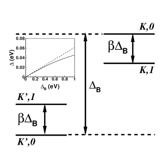
Figure 1: Non-interacting energy levels in Landau level $N=0.$ The inset shows the behavior of the gap evaluated in the original (solid line) and two-band (dashed line) models with bias.

III HARTREE-FOCK HAMILTONIAN

We now add the Coulomb interaction to the non-interacting Hamiltonian $H_{\xi\mathbf{K}}^{0}$. We assume that the magnetic field is strong enough so that we can restrict the Hilbert space to the $N=0$ Landau level and neglect Landau level mixing. We also assume the 2DEG to be fully spin polarized (we comment on this later). We write the electron field operator as

$$\Psi_{\mathbf{K}}\left(\mathbf{r}\right) = \sum_{X}\left(\begin{array}[]{c}0\\ h_{0,X}\left(\mathbf{r}\right)\end{array}\right)c_{K,X,0}$$ (20)

$$+\sum_{X}\left(\begin{array}[]{c}0\\ h_{1,X}\left(\mathbf{r}\right)\end{array}\right)c_{K,X,1}$$

and

$$\Psi_{\mathbf{K}^{\prime}}\left(\mathbf{r}\right) = \sum_{X}\left(\begin{array}[]{c}h_{0,X}\left(\mathbf{r}\right)\\ 0\end{array}\right)c_{K^{\prime},X,0}$$ (26)

$$+\sum_{X}\left(\begin{array}[]{c}h_{1,X}\left(\mathbf{r}\right)\\ 0\end{array}\right)c_{K^{\prime},X,1},$$

so that the Hartree-Fock Hamiltonian is given by (here and in the rest of this paper, we use the convention that repeated indices are summed over)

$$H_{HF}=N_{\phi}E_{a,n}\rho_{n,n}^{a,a}\left(0\right)$$ (27)

$$+N_{\phi}\overline{\sum_{\mathbf{q}}}H_{n_{1},n_{2},n_{3},n_{4}}^{a,b}\left(\mathbf{q}\right)\left\langle\rho_{n_{1},n_{2}}^{a,a}\left(-\mathbf{q}\right)\right\rangle\rho_{n_{3},n_{4}}^{b,b}\left(\mathbf{q}\right)$$

$$-N_{\phi}\sum_{\mathbf{q}}X_{n_{1},n_{4},n_{3},n_{2}}^{a,b}\left(\mathbf{q}\right)\left\langle\rho_{n_{1},n_{2}}^{a,b}\left(-\mathbf{q}\right)\right\rangle\rho_{n_{3},n_{4}}^{b,a}\left(\mathbf{q}\right),$$

where $N_{\phi}$ is the Landau level degeneracy and all energies are measured in units of $e^{2}/\kappa\ell$ where $\kappa$ is the effective dielectric constant at the position of the graphene layers. The single-particle energies $E_{a,n}$ include capacitive contributions and are defined by

$$E_{a,n}=\frac{1}{2}a\Delta_{B}-a\beta\Delta_{B}n+\left[\frac{\widetilde{\nu}}{2}\frac{d}{\ell}-\widetilde{\nu}_{a}\frac{d}{\ell}\right],$$ (28)

with $\widetilde{\nu}_{a}$ the number of filled levels in valley $a$, $\widetilde{\nu}=\nu+4$ the total number of filled levels, $a,b=\pm 1$ the valley (or equivalently layer) index and $n=0,1$ for the two orbital state indices. In deriving Eq. (27), we have taken into account a neutralizing positive background so that the $\mathbf{q}=0$ contribution is absent in the Hartree term. This convention is indicated by the bar over the summation. Note that for positive bias, the bottom layer ($\mathbf{K}^{\prime}$ valley) is at a lower potential than the top layer ($\mathbf{K}$ valley).

The density operators in Eq. (27), are defined by

$$\rho_{n_{1},n_{2}}^{a,b}\left(\mathbf{q}\right) = \frac{1}{N_{\phi}}\sum_{X_{1},X_{2}}e^{-\frac{i}{2}q_{x}\left(X_{1}+X_{2}\right)}$$

$$\times c_{a,X_{1},n_{1}}^{\dagger}c_{b,X_{2},n_{2}}\delta_{X_{1},X_{2}+q_{y}\ell^{2}},$$

where $c_{a,X_{1},n_{1}}^{\dagger}$ creates an electron in state $\left(a,X_{1},n_{1}\right)$ in the Landau gauge. The intralayer $\left(H,X=H^{a,a},X^{a,a}\right)$ and inter-layer $\left(\widetilde{H},\widetilde{X}=H^{a\neq b},X^{a\neq b}\right)$ Hartree and Fock interactions are given by

$$H_{n_{1},n_{2},n_{3},n_{4}}\left(\mathbf{q}\right) = \frac{1}{q\ell}K_{n_{1},n_{2}}\left(\mathbf{q}\right)K_{n_{3},n_{4}}\left(-\mathbf{q}\right),$$ (30)

$$X_{n_{1},n_{2},n_{3},n_{4}}\left(\mathbf{q}\right) = \int\frac{d\mathbf{p}\ell^{2}}{2\pi}H_{n_{1},n_{2},n_{3},n_{4}}\left(\mathbf{p}\right)e^{i\mathbf{q}\times\mathbf{p}\ell^{2}},$$ (31)

and

$$\widetilde{H}_{n_{1},n_{2},n_{3},n_{4}}\left(\mathbf{q}\right) = H_{n_{1},n_{2},n_{3},n_{4}}\left(\mathbf{q}\right)e^{-qd},$$ (32)

$$\widetilde{X}_{n_{1},n_{2},n_{3},n_{4}}\left(\mathbf{q}\right) = \int\frac{d\mathbf{p}\ell^{2}}{2\pi}\widetilde{H}_{n_{1},n_{2},n_{3},n_{4}}\left(\mathbf{p}\right)e^{i\mathbf{q}\times\mathbf{p}\ell^{2}},$$ (33)

where $d=3.337$ Å is the inter-layer separation in the Bernal stacking. The form factors which appear here,

$$K_{0,0}\left(\mathbf{q}\right) = \exp\left(\frac{-q^{2}\ell^{2}}{4}\right),$$ (34)

$$K_{1,1}\left(\mathbf{q}\right) = \exp\left(\frac{-q^{2}\ell^{2}}{4}\right)\left(1-\frac{q^{2}\ell^{2}}{2}\right),$$ (35)

$$K_{1,0}\left(\mathbf{q}\right) = \left(\frac{\left(q_{y}+iq_{x}\right)\ell}{\sqrt{2}}\right)\exp\left(\frac{-q^{2}\ell^{2}}{4}\right),$$ (36)

$$K_{0,1}\left(\mathbf{q}\right) = \left(\frac{\left(-q_{y}+iq_{x}\right)\ell}{\sqrt{2}}\right)\exp\left(\frac{-q^{2}\ell^{2}}{4}\right),$$ (37)

capture the character of the two different orbital states. Detailed expressions for the Hartree and Fock interactions parameters are given in Appendix A.

IV ORDER PARAMETERS AT INTEGER FILLINGS

The states with no pseudospin texture at integer filling factors have uniform electronic density and density-matrices that vanish for $\mathbf{q}\neq 0$. Letting $\left\langle\rho_{n_{1},n_{2}}^{a,b}\left(\mathbf{q}=0\right)\right\rangle\rightarrow$ $\left\langle\rho_{n_{1},n_{2}}^{a,b}\right\rangle,$ the Hamiltonian of Eq. (27) reduces to

$$H_{HF} = N_{\phi}E_{a,n}\rho_{n,n}^{a,a}$$

$$-N_{\phi}X_{n_{1},n_{4},n_{3},n_{2}}^{a,b}\left(0\right)\left\langle\rho_{n_{1},n_{2}}^{a,b}\right\rangle\rho_{n_{3},n_{4}}^{b,a}.$$

These order parameters are conveniently calculated by defining the time-ordered Matsubara Green’s function

$$G_{n_{1},n_{2}}^{a,b}\left(\tau\right)=-\frac{1}{N_{\phi}}\sum_{X}\left\langle T_{\tau}c_{a,n_{1},X}\left(\tau\right)c_{b,n_{2},X}^{\dagger}\left(0\right)\right\rangle,$$ (39)

since, at time zero, we have

$$G_{n_{1},n_{2}}^{a,b}\left(\tau=0^{-}\right)=\left\langle\rho_{n_{2},n_{1}}^{b,a}\right\rangle.$$ (40)

In the Hartree-Fock approximation, the equation of motion for the single-particle Green’s function is

$$\left[\hslash i\omega_{n}-\left(E_{a,n_{1}}-\mu\right)\right]G_{n_{1},n_{2}}^{a,b}\left(\omega_{n}\right)$$ (41)

$$+U_{n_{1},n_{3}}^{a,c}G_{n_{3},n_{2}}^{c,b}\left(\omega_{n}\right)=\hslash\delta_{a,b}\delta_{n_{1},n_{2}},$$

where $\omega_{n}$ is a fermionic Matsubara frequency and

$$U_{n_{1},n_{3}}^{a,c}=X_{n,n_{3},n_{1},n^{\prime}}^{a,c}\left(0\right)\left\langle\rho_{n,n^{\prime}}^{c,a}\right\rangle.$$ (42)

The system of Eqs. (41) can be solved in an iterative way by using some initial values for the parameters $\left\{\left\langle\rho_{n_{2},n_{1}}^{b,a}\right\rangle\right\}.$ In Ref. BarlasPRL, , we solved this equation keeping valley, orbital, and spin indices. We showed that the solutions of the Hartree-Fock equations for the balanced bilayer ($\Delta_{B}=0$) follow a Hund’s rules behavior. The spin polarization is maximized first, then the layer polarization is maximized to the greatest extent possible, and finally the orbital polarization is maximized to the extent allowed by the first two rules. In the absence of bias, the ordering of the first four states (with spin up) is given by

$$\left|S,0\right\rangle = \frac{1}{\sqrt{2}}\left|K,0\right\rangle+\frac{1}{\sqrt{2}}\left|K^{\prime},0\right\rangle,$$ (43)

$$\left|S,1\right\rangle = \frac{1}{\sqrt{2}}\left|K,1\right\rangle+\frac{1}{\sqrt{2}}\left|K^{\prime},1\right\rangle,$$ (44)

$$\left|AS,0\right\rangle = \frac{1}{\sqrt{2}}\left|K,0\right\rangle-\frac{1}{\sqrt{2}}\left|K^{\prime},0\right\rangle,$$ (45)

$$\left|AS,1\right\rangle = \frac{1}{\sqrt{2}}\left|K,1\right\rangle-\frac{1}{\sqrt{2}}\left|K^{\prime},1\right\rangle,$$ (46)

in this order. The next four states follow the same order but with spin down. The occupation of these eight states are given by the filling factor $\nu$ ranging from $\nu=-3$ (state $\left|S,0\right\rangle$ with spin up fully filled) to $\nu=+4$ (all eight states filled).

To simplify the notation, we define

$$\left|K,0\right\rangle \rightarrow \left|1\right\rangle,$$ (47)

$$\left|K,1\right\rangle \rightarrow \left|2\right\rangle,$$

$$\left|K^{\prime},0\right\rangle \rightarrow \left|3\right\rangle,$$

$$\left|K^{\prime},1\right\rangle \rightarrow \left|4\right\rangle,$$

so that $\left\langle\rho_{n_{2},n_{1}}^{b,a}\right\rangle\rightarrow\left\langle\rho_{i,j}\right\rangle$ with $i,j=1,2,3,4.$

It is easy, using Eq. (41), to prove the sum rules

$$\sum_{j=1}^{4}\left|\left\langle\rho_{i,j}\right\rangle\right|^{2}=\nu_{i},$$ (48)

where

$$\nu_{i}=\left\langle\rho_{i,i}\right\rangle.$$ (49)

V COLLECTIVE MODES IN THE GENERALIZED RANDOM-PHASE APPROXIMATION

In order to compute the collective excitations, we define the two-particle Matsubara Green’s function

$$\chi_{n_{1},n_{2},n_{3},n_{4}}^{a,b,c,d}\left(\mathbf{q},\tau\right)$$

$$= -N_{\phi}\left\langle T_{\tau}\rho_{n_{1},n_{2}}^{a,b}\left(\mathbf{q,}\tau\right)\rho_{n_{3},n_{4}}^{c,d}\left(-\mathbf{q},0\right)\right\rangle$$

$$+N_{\phi}\left\langle\rho_{n_{1},n_{2}}^{a,b}\left(\mathbf{q}\right)\right\rangle\left\langle\rho_{n_{3},n_{4}}^{c,d}\left(-\mathbf{q}\right)\right\rangle,$$

where again $n_{i}=0,1$ are orbital indices and $a,b,c,d$ are valley indices. To derive the equation of motion for these response functions in the Generalized Random-Phase Approximation (GRPA), we proceed in the following way. We first derive the equation of motion for $\chi$ in the Hartree-Fock Approximation (HFA) using the Heisenberg equation of motion

$$\hslash\frac{\partial}{\partial\tau}\left(\ldots\right)=\left[H-\mu N,\left(\ldots\right)\right],$$ (51)

where $H$ is the Hamiltonian of Eq. (27) with the averages removed, $\mu$ is the chemical potential and $N$ the number operator (not to be confused with the Landau level index). After evaluating the commutators, we linearize the resulting equation by writing $\rho\left(\mathbf{q}\right)\rightarrow\left\langle\rho\left(\mathbf{q}\right)\right\rangle_{HFA}+\delta\rho\left(\mathbf{q}\right)$. We get the GRPA equations of motion by keeping the terms up to linear order in $\delta\rho\left(\mathbf{q}\right).$ In the homogeneous states at integer fillings, $\left\langle\rho\left(\mathbf{q}\right)\right\rangle_{HF}=\left\langle\rho\left(\mathbf{q}\right)\right\rangle_{HF}\delta_{\mathbf{q},0},$ so that we get the set of equations

$$\left[i\hslash\Omega_{n}-\left(E_{b,n_{2}}-E_{a,n_{1}}\right)\right]\chi_{n_{1},n_{2},n_{3},n_{4}}^{\left(0\right)a,b,c,d}\left(\mathbf{q},\Omega_{n}\right)$$

$$= \hslash\left\langle\rho_{n_{1},n_{4}}^{a,d}\right\rangle\delta_{n_{2},n_{3}}\delta_{b,c}-\hslash\left\langle\rho_{n_{3},n_{2}}^{c,b}\right\rangle\delta_{a,d}\delta_{n_{1},n_{4}}$$

$$+X_{n_{1}^{\prime},n_{1},n_{3}^{\prime},n_{2}^{\prime}}^{a,b^{\prime}}\left(0\right)\left\langle\rho_{n_{1}^{\prime},n_{2}^{\prime}}^{a,b^{\prime}}\right\rangle\chi_{n_{3}^{\prime},n_{2},n_{3},n_{4}}^{\left(0\right)b^{\prime},b,c,d}\left(\mathbf{q},\Omega_{n}\right)$$

$$-X_{n_{1}^{\prime},n_{4}^{\prime},n_{2},n_{2}^{\prime}}^{a^{\prime},b}\left(0\right)\left\langle\rho_{n_{1}^{\prime},n_{2}^{\prime}}^{a^{\prime},b}\right\rangle\chi_{n_{1},n_{4}^{\prime},n_{3},n_{4}}^{\left(0\right)a,a^{\prime},c,d}\left(\mathbf{q},\Omega_{n}\right),$$

and

$$\chi_{n_{1},n_{2},n_{3},n_{4}}^{a,b,c,d}\left(\mathbf{q};\Omega_{n}\right)$$

$$= \chi_{n_{1},n_{2},n_{3},n_{4}}^{\left(0\right)a,b,c,d}\left(\mathbf{q};\Omega_{n}\right)$$

$$+\frac{1}{\hslash}\chi_{n_{1},n_{2},n_{5},n_{6}}^{\left(0\right)a,b,e,e}\left(\mathbf{q};\Omega_{n}\right)H_{n_{5},n_{6},n_{7},n_{8}}^{e,g}\left(\mathbf{q}\right)$$

$$\times\chi_{n_{7},n_{8},n_{3},n_{4}}^{g,g,c,d}\left(\mathbf{q};\Omega_{n}\right)$$

$$-\frac{1}{\hslash}\chi_{n_{1},n_{2},n_{5},n_{6}}^{\left(0\right)a,b,e,f}\left(\mathbf{q};\Omega_{n}\right)X_{n_{5},n_{8},n_{7},n_{6}}^{e,f}\left(\mathbf{q}\right)$$

$$\times\chi_{n_{7},n_{8},n_{3},n_{4}}^{f,e,c,d}\left(\mathbf{q};\Omega_{n}\right),$$

where $\Omega_{n}$ is a bosonic Matsubara frequency. The retarded response functions are obtained, as usual, by taking the analytic continuation $i\Omega_{n}\rightarrow\omega+i\delta.$

By defining super indices $A,B=1,2,3,...,16$ representing the combinations $(a,n_{1};b,n_{2}),\left(c,n_{3};d,n_{4}\right),$ etc., we can represent the response functions and interactions matrices as $16\times 16$ matrices and then write the GRPA equation in the matrix form:

$$\left[\left(\omega+i\delta\right)I-F\left(\mathbf{q}\right)\right]\chi\left(\mathbf{q},\omega\right)=B\left(\mathbf{q}\right),$$ (54)

where $B,I,F,\chi$ are $16\times 16$ matrices (with $I$ the unit matrix). The matrices $F\left(\mathbf{q}\right)$ and $B\left(\mathbf{q}\right)$ depend on the $\left\langle\rho_{n_{2},n_{1}}^{b,a}\right\rangle^{\prime}s$ evaluated in the HFA. We will give later the precise form of these matrices for the phases studied in this paper.

The frequencies of the collective excitations are given by the eigenvalues of the matrix $F\left(\mathbf{q}\right).$ There are in total 4 zero modes, corresponding to unphysical intra-level transitions, and 12 non-zero modes corresponding to inter-level transitions. The latter occur in six positive-negative energy pairs, corresponding to excitation and deexcitation partners. Of the six collective excitations identified in this way, three are Pauli-blocked at $\nu=-1$ and appear in our calculations as dispersionless modes that have zero weight in all physical response properties. The three remaining excitation modes are physical and for $\nu=-1$ correspond to the interaction-coupled transitions indicated in Fig. 2. Note that, in the limit $q\rightarrow\infty$, $H^{e,g},X^{e,f}\rightarrow 0$ so that Eq. (V) gives $\chi\rightarrow\chi^{0}$. In this limit, the collective mode frequencies correspond to transitions between eigenstates of the Hartree-Fock Hamiltonian $H_{HF}$ as illustrated in Fig. 2 for the case $\nu=-1$ and zero bias. The energy of these eigenstates include the non-interacting energies and the self-energy corrections. The $\omega\left(\mathbf{q}=0\right)$ limit of these sames modes, however, also includes the polarization and excitonic corrections that, in a Feynman diagram description of the GRPA, are captured by bubble and ladder diagram summations. These effects make the modes dispersive.

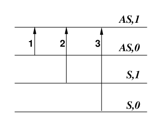
Figure 2: At $\nu=-1$, the first three energy states of the Hartree-Fock Hamiltonian are filled and the only possible transitions are those indicated by the three arrows. The frequency of these transitions corresponds to the frequency of the collective excitations calculated in the GRPA in the limit in which the wavevector $q\rightarrow\infty.$ We illustrate here the case of zero bias.

VI PHASE DIAGRAM AT FILLING FACTOR $\nu=-1$

The properties of the ground state at $\nu=-3$ have been studied in detail in Ref. yafis2, . At zero bias, the ground state has all electrons in the $\left|S,0\right\rangle$ state and can be described as an $XY$ layer-pseudospin ferromagnet with orbital character $n=0$. The bias $\Delta_{B}$ acts as an effective external magnetic field that forces the layer pseudospins out of the $x-y$ plane. Above a critical bias $\Delta_{B}^{\left(c\right)}$, all electrons are in the bottom layer and the layer-pseudospin is correspondingly fully polarized. The ground state is then given by $\left|K^{\prime},0\right\rangle$ and is unchanged if the bias is further increased. The $\nu=-1$ state on which we focus here differs from the $\nu=-3$ state because of a competition between single-particle and interaction energy effects which emerges only in the former case. As illustrated in Fig. (1), single-particle effects captured by the bilayer effective Hamiltonian favor occupation of the $n=1$ orbital when three of the octet’s eight levels are occupied ($\nu=-1$). Note that this tendency is independent of the sign of $\Delta_{B}$. Exchange interactions, on the other hand, always favor a state in which as many $n=0$ orbitals as possible are occupied. As we explain below, a compromise is reached by forming a state with coherence between $n=0$ and $n=1$ orbitals. This physics is enriched by the same tendency toward interlayer coherence which occurs at $\nu=-3$ andcoherencerefs in semiconductor bilayers. Indeed, our calculations show that the phase diagram at $\nu=-1$ is much more complex than at $\nu=-3$.

VI.1 Inter-layer-coherent state

At zero bias, numerical solution of the HFA equations leads to occupied $\left|S,0\right\rangle,\left|S,1\right\rangle,$ and $\left|AS,0\right\rangle$ states. The order parameters are then given by

$$\nu_{1} = \nu_{3}=1,$$ (55)

$$\nu_{2} = \nu_{4}=\frac{1}{2},$$

$$\left\langle\rho_{2,4}\right\rangle = \left\langle\rho_{4,2}\right\rangle=\frac{1}{2}.$$

The ground state is an $XY$ layer-pseudospin ferromagnet with orbital character $n=1.$ The Hamiltonian is invariant with respect to the orientation of the pseudospins in the $x-y$ plane so that this phase supports a Goldstone mode. The choice of phase in Eq. (55) has the pseudospins pointing along the $x$ axis. At finite bias $\Delta_{B}<\Delta_{B}^{(1)}$, the pseudospins are pushed out the $x-y$ plane i.e. the two layers have unequal population. The occupation of the four states are in this case

$$\nu_{1}=\nu_{3}=1,$$ (56)

and

$$\nu_{2}=1-\nu_{4}=\frac{1}{2}\left(1-\frac{\Delta_{B}}{\Delta_{B}^{\left(1\right)}}\right),$$ (57)

with inter-layer coherence reflected by

$$\left\langle\rho_{2,4}\right\rangle=\left\langle\rho_{4,2}\right\rangle=\sqrt{\nu_{2}-\nu_{2}^{2}}.$$ (58)

We define the critical bias $\Delta_{B}^{\left(1\right)}$ as the bias at which the inter-layer coherence $\left\langle\rho_{2,4}\right\rangle=0.$ It is given by

$$\Delta_{B}^{\left(1\right)}=\frac{-3x_{7}\left(0\right)+2\widetilde{x}_{16}\left(0\right)+2\frac{d}{\ell}}{2-4\beta},$$ (59)

where the Fock interactions $x_{i}\left(\mathbf{q}\right)$ and $\widetilde{x}_{i}\left(\mathbf{q}\right)$ are defined in Appendix A. As an example, for $B=10$ T, $\Delta_{B}^{\left(1\right)}=0.00205\,e^{2}/\kappa\ell.$

The energy of this inter-layer-coherent state (ICS) for $\Delta_{B}<\Delta_{B}^{(1)}$ is

$$\frac{E_{HF}^{(1)}}{N} = \frac{1}{3}\Delta_{B}\left(1-2\beta\right)\left\langle P_{z,1}\right\rangle$$

$$-\frac{1}{3}x_{1}\left(0\right)-\frac{1}{3}x_{7}\left(0\right)-\frac{1}{12}x_{16}\left(0\right)$$

$$+\frac{1}{3}\left(\frac{d}{\ell}-x_{16}\left(0\right)\right)\left\langle P_{z,1}\right\rangle^{2}$$

$$-\frac{1}{3}\widetilde{x}_{16}\left(0\right)\left\langle\mathbf{P}_{\bot,1}\right\rangle^{2},$$

where the components of the layer pseudospin are given by

$$\left\langle P_{z,1}\right\rangle = \frac{\nu_{2}-\nu_{4}}{2}=-\frac{1}{2}\frac{\Delta_{B}}{\Delta_{B}^{\left(1\right)}},$$ (61)

$$\left\langle\mathbf{P}_{\bot,1}\right\rangle^{2} = \left\langle P_{x,1}\right\rangle^{2}+\left\langle P_{y,1}\right\rangle^{2}=\left|\left\langle\rho_{2,4}\right\rangle\right|^{2},$$ (62)

with the convention that pseudospin up is state $\left|2\right\rangle$ while pseudospin down is state $\left|4\right\rangle.$

VI.2 Inter-orbital-coherent state

The HFA equations have a separate set of solutions, favored at larger bias voltages, in which the lower layer is maximally occupied, and the ground state has upper-layer orbital coherence instead of inter-layer coherence. This solution has

$$\nu_{3}=\nu_{4}=1,$$ (63)

$$\nu_{2}=1-\nu_{1}=\frac{\Delta_{B}}{\Delta_{B}^{(2)}},$$ (64)

and inter-orbital coherence is signalled by the density-matrix components

$$\left\langle\rho_{1,2}\right\rangle=\left\langle\rho_{2,1}\right\rangle=\sqrt{\nu_{2}-\nu_{2}^{2}}.$$ (65)

Here

$$\Delta_{B}^{(2)}=\frac{x_{4}\left(0\right)}{2\beta}$$ (66)

is the critical bias above which all charges in the upper layer are transferred to state $\left|2\right\rangle$ and the orbital coherence is lost. In a pseudospin model with the convention: pseudospin up for state $\left|1\right\rangle$ and pseudospin down for state $\left|2\right\rangle$, the orbital pseudospin components are given by

$$\left\langle S_{z,K}\right\rangle = \frac{\nu_{1}-\nu_{2}}{2},$$ (67)

$$\left\langle\mathbf{S}_{\bot,1}\right\rangle = \left\langle S_{x,1}\right\rangle\widehat{\mathbf{x}}+\left\langle S_{y,1}\right\rangle\widehat{\mathbf{y}},$$ (68)

$$\left\langle S_{+,K}\right\rangle = \left\langle S_{x,K}\right\rangle+i\left\langle S_{y,K}\right\rangle=\left\langle\rho_{1,2}\right\rangle.$$ (69)

This orbital-coherent phase has all pseudospins tilted slightly away from the $z$ axis by an angle

$$\cos\theta_{B}=1-2\frac{\Delta_{B}}{\Delta_{B}^{(2)}}.$$ (70)

At the critical bias $\Delta_{B}^{(2)}$, $\theta_{B}=\pi.$ This critical bias $\Delta_{B}^{(2)}$ is very large; at $B=10$ T, $\Delta_{B}^{(2)}\approx 5e^{2}/\kappa\ell$ which is near the limit of validity of the effective two-band model i.e. $\hslash\omega_{c}<\gamma_{1}$. For $\Delta_{B}>\Delta_{B}^{(2)}$, all electrons are in state $\left|2\right\rangle$ and there is no further change with bias of the ground state.

The orbital-coherent state (OCS) has an energy given by

$$\frac{E_{HF}^{(2)}}{N} = \frac{1}{3}\left[-\left(1-\beta\right)\frac{\Delta_{B}}{2}+\beta\Delta_{B}\left\langle S_{z,K}\right\rangle\right]+\frac{1}{12}\frac{d}{\ell}$$

$$-\frac{5}{24}\left[x_{1}\left(0\right)+x_{16}\left(0\right)+2x_{7}\left(0\right)\right]$$

$$-\frac{1}{6}\left[x_{1}\left(0\right)-x_{16}\left(0\right)\right]\left\langle S_{z,K}\right\rangle$$

$$-\frac{1}{6}\left[x_{1}\left(0\right)+x_{16}\left(0\right)-4x_{7}\left(0\right)\right]\left\langle S_{z,K}\right\rangle^{2}$$

$$-\frac{1}{3}x_{4}\left(0\right)\left\langle\mathbf{S}_{\bot,K}\right\rangle^{2}.$$

This energy is independent of the azimuthal angle $\varphi$ of the pseudospin vector. We can thus, without loss of generality, take $\left\langle\rho_{1,2}\right\rangle$ as real.

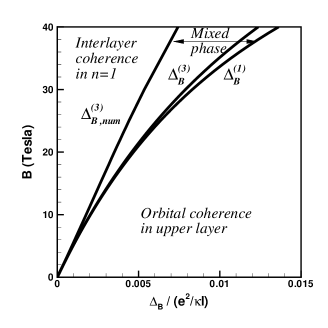
Figure 3: Phase diagram of the 2DEG in a graphene bilayer at $\nu=-1.$

VI.3 Mixed state

Eqs. (VI.1) and (VI.2) give $E_{HF}^{(2)}<E_{HF}^{(1)}$ above a critical bias $\Delta_{B}^{(3)}<\Delta_{B}^{(1)}$. For biases $\Delta\in\left[\Delta_{B}^{(3)},\Delta_{B}^{(1)}\right],$ a mixed state with both inter-orbital and inter-layer coherence would be lower in energy than a state with only interlayer coherence. Solving the full Hartree-Fock equations, we find that the crossover from the inter-layer coherent state to the inter-orbital coherent state occurs continuously via an intermediate state with both orders. The boundaries of the intermediate phase must be determined numerically. We find that the boundaries of this mixed state (MS) are given on the left by a new critical bias $\Delta_{B,num}^{(3)}<\Delta_{B}^{(3)}$ and on the right by $\Delta_{B}^{(1)}.$ The intermediate phase region broadens with magnetic field as can be seen in Fig. 3.

Figure 4 shows the evolution of the inter-layer coherence $\left\langle\rho_{2,4}\right\rangle$ and the orbital coherence $\left\langle\rho_{1,2}\right\rangle$ with bias at magnetic field $B=10$ T. The orbital coherence sets in before the inter-layer coherence decreases to zero thus creating the mixed state region identified in this figure by a non zero value of the density-matrix component $\left\langle\rho_{1,4}\right\rangle$. (Note that $\left\langle\rho_{1,2}\right\rangle$ is not given by Eq. (65) in the mixed state.) The coherences $\left\langle\rho_{1,4}\right\rangle$ and $\left\langle\rho_{2,3}\right\rangle,$ which involve a mixing of valley and as well as orbital indices, are non-zero only in the intermediate mixed-state region of the phase diagram. All density-matrix components vary continuously with inter-layer bias.

As can be seen from Figs. 3 and 4, the orbital-coherent phase starts at $\Delta_{B}^{(1)}$ with a finite orbital coherence $\left\langle\rho_{1,2}\right\rangle$. Were it not for the presence of the inter-layer-coherent and mixed states, $\left\langle\rho_{1,2}\right\rangle$ would start at zero bias and be given by Eq. (65) for all biaises. The mixed and inter-layer coherent states are confined to relatively small inter-layer bias voltages; at larger values of $\Delta_{B}$ the ground state is a relatively simple state with only orbital coherence. The exploration of collective excitation properties of this state is one key objective of this paper.

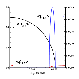
Figure 4: (Color online) Evolution of the inter-layer $\left\langle\rho_{2,4}\right\rangle$ and inter-orbital $\left\langle\rho_{1,2}\right\rangle$ coherences (left axis) with bias at filling factor $\nu=-1$ and magnetic field $B=10$ T. On the right axis, one of the non zero coherences $\left\langle\rho_{1,4}\right\rangle$ in the mixed state.

VII COLLECTIVE MODES IN THE INTER-LAYER COHERENT STATE

The density-matrix equations of motions which describe the three $\nu=-1$ spin-diagonal dispersive collective modes (see Fig. 2) are usually simplest when written in the basis of the bonding and antibonding single-particle Hartree-Fock eigenstates. For the interlayer coherent state (ICS) (the ground state for $\Delta_{B}<$ $\Delta_{B,num}^{(3)}$) we find that,

$$\left(I\left(\omega+i\delta\right)-F_{1}\right)\left(\begin{array}[]{c}ie^{-i\theta_{\mathbf{q}}}\rho_{AB1,B0}\\ ie^{i\theta_{\mathbf{q}}}\rho_{B0,AB1}\\ \rho_{AB1,B1}\\ \rho_{B1,AB1}\\ ie^{i\theta_{\mathbf{q}}}\rho_{AB0,AB1}\\ ie^{-i\theta_{\mathbf{q}}}\rho_{AB1,AB0}\end{array}\right)=\left(\begin{array}[]{c}0\\ 0\\ 0\\ 0\\ 0\\ 0\end{array}\right),$$ (72)

where $\theta_{\mathbf{q}}$ is the angle between the two-dimensional wavevector $\mathbf{q}$ and the $x$ axis, and $B$ and $AB$ refer to the states

$$\left|B,n,X\right\rangle = g_{-}\left|K,n,X\right\rangle+g_{+}\left|K^{\prime},n,X\right\rangle,$$ (73)

$$\left|AB,n,X\right\rangle = g_{+}\left|K,n,X\right\rangle-g_{-}\left|K^{\prime},n,X\right\rangle,$$ (74)

where $n=0,1,$

$$g_{\pm}=\sqrt{\frac{1\pm\sigma}{2}},$$ (75)

and

$$\sigma=\frac{\Delta_{B}}{\Delta_{B}^{\left(1\right)}}.$$ (76)

The matrix $F_{1}$ depends only on the modulus of the wavevector $\mathbf{q}$ so that the dispersions are isotropic. This matrix is given by

$$F_{1}\left(q\right)=\frac{1}{2}\left(\begin{array}[]{cccccc}-A-\sigma^{2}B&fH&-N+\sigma^{2}J&-fJ&\sigma\sqrt{f}H&-\sigma\sqrt{f}G\\ -fH&A+\sigma^{2}B&fJ&N-\sigma^{2}J&\sigma\sqrt{f}G&-\sigma\sqrt{f}H\\ -N+\sigma^{2}J&-fJ&-C-\sigma^{2}D&fM&-\sigma\sqrt{f}J&-\sigma\sqrt{f}J\\ fJ&N-\sigma^{2}J&-fM&C+\sigma^{2}D&\sigma\sqrt{f}J&\sigma\sqrt{f}J\\ -\sigma\sqrt{f}H&\sigma\sqrt{f}G&\sigma\sqrt{f}J&\sigma\sqrt{f}J&-E-\sigma^{2}F&K-\sigma^{2}H\\ -\sigma\sqrt{f}G&\sigma\sqrt{f}H&-\sigma\sqrt{f}J&-\sigma\sqrt{f}J&-K+\sigma^{2}H&E+\sigma^{2}F\end{array}\right),$$ (77)

where

$$f=1-\sigma^{2}$$ (78)

The variables in this matrix are defined in Appendix B.

The GRPA dispersions for the three collective modes are shown in Fig. 5 for zero bias and a magnetic field of $B=10$ T. In the limit $q\rightarrow\infty$, the frequencies of the dispersive modes correspond to transitions between the HFA energy levels indicated in Fig. 2 as expected. Mode $2$ in Fig. 5 is a Goldstone mode consisting of a precession of the inter-layer pseudospin $\mathbf{P}_{1}$ around the $x$ axis. We refer to it as the inter-layer pseudospin mode (IPM). Mode $1$ is an orbital pseudospin mode (OPM) consisting of a precession of the orbital pseudospins around their local equilibrium position. Mode $3$ involves both a layer and orbital pseudospin flip and has a large gap. At finite bias, the $3$ dispersive modes in Fig. 2 are coupled together while at zero bias, modes $2$ and $3$ completely decouple from mode $1$ as is clear from Eq. (77).

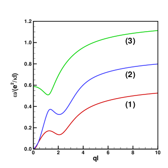
Figure 5: (Color online) Dispersion relations of the collective modes at $\nu=-1$ in the inter-layer coherent phase at zero bias and for $B=10$ T. The numbers refer to the transitions indicated in Fig. 2.

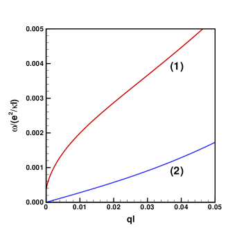
Figure 6: (Color online) Long-wavelength (small $q$) dispersion relation of the collective modes in the inter-layer coherent phase at $\nu=-1$ for zero bias and for $B=10$ T. Mode $1$ is the orbital pseudospin mode while mode $2$ is the inter-layer pseudospin mode.

From Eq. (77), it is easy to see that the dispersion of the OPM at zero bias (given by the $2\times 2$ block in the lower right of the matrix $F_{1}$) is given by

$$\omega_{OPM}\left(\mathbf{q}\right)=\frac{1}{2}\sqrt{E^{2}\left(\mathbf{q}\right)-K^{2}\left(\mathbf{q}\right)},$$ (79)

and has a gap given by (see Appendix B)

$$\omega_{OPM}\left(0\right)=\frac{1}{2}\left[x_{1}\left(0\right)-\widetilde{x}_{1}\left(0\right)-x_{16}\left(0\right)+\widetilde{x}_{16}\left(0\right)\right].$$ (80)

This gap is small but visible in Fig. 6. We find numerically, that as the bias is increased, the gap $\omega_{OPM}\left(0\right)$ decreases until it reaches zero at the phase boundary of the mixed state.

The dispersion of the IPM is linear in $q$ for $q\ell<d/\ell$ (with $d/\ell\approx 0.04$ for $B=10$T) as in a semiconductor bilayerspielmanPRL . This findings differ qualitatively from the $\nu=-3,$ case for which we foundyafis2 an IPM with $q^{2}$ dispersion and a gapless OPM. At $\nu=-3$ and zero bias, the $\left|S,0\right\rangle$ level is filled. The $q^{2}$ IPM dispersion in that case occurs because the possibility of mixing $n=1$ wavefunctions with $\left|AS,0\right\rangle$ wavefunctions in excited states allows the inter-layer phase stiffness to vanish. At $\nu=-1$, it is not possible to make the corresponding admixture.

In pseudospin language, a finite bias pushes the layer pseudospins $\mathbf{P}_{1}$ out of the $x-y$ plane but the Hamiltonian of the system remains independent of the orientation of the perpendicular component of these pseudospins in the $x-y$ plane. The IPM therefore remains gapless for $\Delta_{B}<\Delta_{B,num}^{(3)}.$ It acquires a gap in the mixed and OCS. At filling factor $\nu=-3$, the inter-layer-pseudospin mode becomes unstable at finite bias. This indicates that the uniform inter-layer-coherent state cannot in fact be the ground state at finite bias. We see no such instability at $\nu=-1.$

In the absence of a bias, Eq. (77) shows that modes $2$ and $3$ are coupled through $N$ and $J.$ These interactions involves the Coulomb interaction matrix elements $\widehat{X}_{0,1,1,1}\left(\mathbf{q}\right)$ and $\widehat{H}_{0,1,1,1}\left(\mathbf{q}\right)$ (see Appendix A for their definitions). These interactions do not conserve total $n=0$ or $n=1$ quantum numbers. Such interactions do not occur in usual semiconductor 2DEG where spin and layer pseudospin indices are conserved.

VIII COLLECTIVE MODES IN THE ORBITAL COHERENT STATE

In this section, we consider collective excitations of the orbital coherent state (OCS) which is the ground state in the region $\Delta_{B}^{\left(1\right)}<\Delta_{B}<\Delta_{B}^{(2)}$, which covers the large region of bias voltages from small values to the largest values for which the two-band effective model applies. The occurrence of the interesting OCS state at high bias voltages is a consequence of competition between single-particle and interaction effects as explained earlier. By studying its collective interactions we reveal a Dzyaloshinskii-Moriya (DM) interaction between orbital pseudospins and demonstrate that for large bias voltages it drives an instability to an orbital pseudospin spiral state.

VIII.1 Electric dipole density

The fact that $\left\langle\rho_{1,2}\right\rangle\neq 0$ in the OCS implies that there is a finite density of electric dipoles in this phase as first pointed out in Ref. shizuya1, . To show this, we write the total electronic density (including the two valleys) as

$$n\left(\mathbf{q}\right)=n_{K}\left(\mathbf{q}\right)+n_{K^{\prime}}\left(\mathbf{q}\right),$$ (81)

where

$$n_{K}\left(\mathbf{q}\right)=N_{\varphi}\sum_{i,j=0,1}K_{i,j}\left(-\mathbf{q}\right)\rho_{i,j}^{K,K}\left(\mathbf{q}\right),$$ (82)

with $\rho_{0,1}^{K,K}=\rho_{1,2}$. The functions $K_{i,j}\left(\mathbf{q}\right)$ are defined in Eqs. (34-37). In our pseudospin langage for the orbital states, we have the relations (for the $K$ valley)

$$\rho^{K}\left(\mathbf{q}\right) = \rho_{0,0}^{K,K}\left(\mathbf{q}\right)+\rho_{1,1}^{K,K}\left(\mathbf{q}\right),$$ (83)

$$\rho_{z}^{K}\left(\mathbf{q}\right) = \frac{1}{2}\left[\rho_{0,0}^{K,K}\left(\mathbf{q}\right)-\rho_{1,1}^{K,K}\left(\mathbf{q}\right)\right],$$ (84)

$$\rho_{+}^{K}\left(\mathbf{q}\right) = \rho_{0,1}^{K,K}\left(\mathbf{q}\right)=\rho_{x}^{K}\left(\mathbf{q}\right)+i\rho_{y}^{K}\left(\mathbf{q}\right)$$ (85)

and so the density operator in the $K$ valley can be written as

$$n_{K}\left(\mathbf{q}\right) = N_{\varphi}\left(1-\frac{q^{2}\ell^{2}}{4}\right)\overline{\rho}_{K}\left(\mathbf{q}\right)$$

$$+N_{\varphi}\left(\frac{q^{2}\ell^{2}}{2}\right)\overline{\rho}_{K,z}\left(\mathbf{q}\right)$$

$$-N_{\varphi}\sqrt{2}iq_{x}\ell\;\overline{\rho}_{K,x}\left(\mathbf{q}\right)$$

$$+N_{\varphi}\sqrt{2}iq_{y}\ell\;\overline{\rho}_{K,y}\left(\mathbf{q}\right),$$

where we have defined $\overline{\rho}_{K}\left(\mathbf{q}\right)=\exp\left(-q^{2}\ell^{2}/4\right)\rho^{K}\left(\mathbf{q}\right)$ and similarly for $\overline{\rho}_{K,i}$ with $i=x,y,z.$

Now, if the 2DEG is in an external electric field $\mathbf{E}\left(\mathbf{r}\right)=-\nabla\phi\left(\mathbf{r}\right),$ we have for the coupling Hamiltonian

$$H_{ext} = -e\int d\mathbf{r}\;n\left(\mathbf{r}\right)\phi\left(\mathbf{r}\right)$$

$$= -\frac{e}{S}N_{\varphi}\sum_{j=K,K^{\prime}}\sum_{\mathbf{q}}e^{i\mathbf{q}\cdot\mathbf{r}}\left[\left(1-\frac{q^{2}\ell^{2}}{4}\right)\overline{\rho}_{j}\left(-\mathbf{q}\right)\right.$$

$$+\left(\frac{q^{2}\ell^{2}}{2}\right)\overline{\rho}_{j,z}\left(-\mathbf{q}\right)$$

$$\left.-\sqrt{2}i\left(q_{x}\ell\;\overline{\rho}_{j,x}\left(-\mathbf{q}\right)+q_{y}\ell\;\overline{\rho}_{j,y}\left(-\mathbf{q}\right)\right)\right]\phi\left(\mathbf{q}\right).$$

With the electric field in the plane of the 2DEG, this coupling can be written, in real space, as

$$H_{ext} = -eN_{\varphi}\sum_{j=K,K^{\prime}}\int d\mathbf{r}\left[\overline{\rho}_{j}\left(\mathbf{r}\right)\phi\left(\mathbf{r}\right)\right.$$

$$-\left.\frac{1}{4}\left(\overline{\rho}_{j}\left(\mathbf{r}\right)\ell^{2}-2\overline{\rho}_{j,z}\left(\mathbf{r}\right)\ell^{2}\right)\left(\mathbf{\nabla}\cdot\mathbf{E}\left(\mathbf{r}\right)\right)\right]$$

$$+\sqrt{2}\ell\int d\mathbf{r}\left[\overline{\rho}_{j,x}\left(\mathbf{r}\right)E_{x}\left(\mathbf{r}\right)-\overline{\rho}_{j,y}\left(\mathbf{r}\right)E_{y}\left(\mathbf{r}\right)\right].$$

The inter-orbital coherence is zero in the $K^{\prime}$ valley and so $\left\langle\overline{\rho}_{K^{\prime},x}\right\rangle,\left\langle\overline{\rho}_{K^{\prime},y}\right\rangle=0.$ Eq. (VIII.1) implies that the dipole density in the 2D plane is

$$\left\langle\overline{\mathbf{d}}_{K}\left(\mathbf{r}\right)\right\rangle=-e\sqrt{2}\ell N_{\varphi}\left(\left\langle\overline{\rho}_{K,x}\left(\mathbf{r}\right)\right\rangle\widehat{\mathbf{x}}-\left\langle\overline{\rho}_{K,y}\left(\mathbf{r}\right)\right\rangle\widehat{\mathbf{y}}\right),$$ (89)

or

$$\left\langle\mathbf{d}_{K}\left(\mathbf{q}\right)\right\rangle = -e\sqrt{2}\ell N_{\varphi}e^{-q^{2}\ell^{2}/4}$$

$$\times\left(\left\langle\rho_{K,x}\left(\mathbf{q}\right)\right\rangle\widehat{\mathbf{x}}-\left\langle\rho_{K,y}\left(\mathbf{q}\right)\right\rangle\widehat{\mathbf{y}}\right).$$

The orientation of the dipole density is set by the phase of the density-matrix component $\left\langle\rho_{0,1}^{K,K}\left(\mathbf{r}\right)\right\rangle=$ $\left\langle\rho_{1,2}\left(\mathbf{r}\right)\right\rangle$ which specifies the phase of the spontaneously established coherence between $n=0$ and $n=1$ orbitals in the ground state. For our choice of the spontaneously established phase of $\left\langle\rho_{1,2}\left(\mathbf{r}\right)\right\rangle$ in Eq. (65), the dipoles are oriented along the $x$ axis. Because the $K^{\prime}$ valley (bottom layer) Landau levels are maximally filled, there is no inter-orbital coherence and therefore no contribution to the electric-dipole density from the $\mathbf{K}^{\prime}$ valley.

VIII.2 Effective pseudospin model

Collective modes dispersions for the OCS are plotted in Fig. 7. For relatively small values of $\Delta_{B}$ they are very similar to those represented in Fig. 5 for the ICS; the main changes occur at small wavevector as can be seen in the inset of Fig. 7. The inter-layer pseudospin mode is gapped in the OCS while the orbital pseudospin mode is gapless, with a very anisotropic dispersion as shown in Fig. 8. We now discuss the physics of the orbital pseudospin mode.

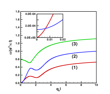
Figure 7: (Color online) Dispersion relations of the collective modes along $q_{x}$ in the orbital-coherent state at filling factor $\nu=-1,$ bias $\Delta_{B}=0.0022$ $e^{2}/\kappa\ell$ and magnetic field $B=10$ T. Mode $1$ is the Goldstone mode due to orbital coherence. Modes $2$ and $3$ involve an inter-layer transition and are gapped. The inset shows the dispersion of mode $1$ (gapless) and mode $2$ (gapped) at small $q_{x}\ell.$

At finite wavevector $\mathbf{q}$, the orbital pseudospin mode (OPM) corresponds to a precession of the orbital pseudospins around their equilibrium orientation in the ground state as illustrated in Fig. 9. The ground state is described by spinors

$$\left|K,B,X\right\rangle=\cos\left(\frac{\theta_{B}}{2}\right)\left|K,0,X\right\rangle+\sin\left(\frac{\theta_{B}}{2}\right)\left|K,1,X\right\rangle,$$ (91)

where $\theta_{B}\in\left[0,\pi\right]$ has been defined in Eq. (70).

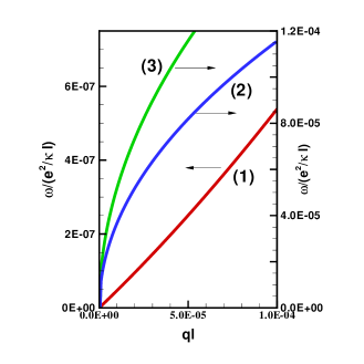
Figure 8: (Color online) Dispersion relations of the collective modes in the orbital-coherent phase at filling factor $\nu=-1$, bias $\Delta_{B}=0.0022$ $e^{2}/\kappa\ell$ and magnetic field $B=10$ T. Curve (1) $q_{y}=0;$ curve (2) $q_{x}=q_{y};$ and curve (3) $q_{x}=0.$

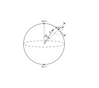
Figure 9: Precession of the orbital pseudospin $\mathbf{S}$ around its equilibrium position with polar angle $\theta_{B}$ and azimuthal angle $\varphi_{B}=0$. This orientation is choosen as the orbital pseudospin quantization axis in the pseudospin wave model. The angle $\theta$ is the polar angle measured from the equilibrium orientation of the pseudospins.

The collective mode corresponds to spatially coherent rotations of this spinor around its ground state value. For this reason, it is convenient to choose the orbital pseudospin quantization axis along the direction $\left|B,0\right\rangle$. In order to do this, we define ‘bonding’ and ‘antibonding’ electron creation operators by

$$b_{B,K,X}^{{\dagger}} = \cos\left(\frac{\theta_{B}}{2}\right)c_{0,X}^{{\dagger}}+\sin\left(\frac{\theta_{B}}{2}\right)c_{1,X}^{{\dagger}},$$ (92)

$$b_{AB,K,X}^{{\dagger}} = \sin\left(\frac{\theta_{B}}{2}\right)c_{0,X}^{{\dagger}}-\cos\left(\frac{\theta_{B}}{2}\right)c_{1,X}^{{\dagger}}.$$ (93)

Below we use the convention that pseudospin up corresponds to state $\left|B,K\right\rangle$ and pseudospin down to state $\left|AB,K\right\rangle$ and we denote the pseudospin by $\mathbf{S}.$

In our GRPA system of equations for the collective modes, the orbital-pseudospin wave mode is decoupled from all other modes. Below we follow one possible strategy for explaining the physics of this mode by comparing our microscopic GRPA equation of motion to the equations of motion of an effective orbital pseudospin model, and using the comparison to identify the effective pseudospin interactions. Since collective modes correspond to small oscillations of the pseudospin around its quantization direction, we can use an effective model which has interactions only between transverse spins. (Quantization direction interactions can be represented as transverse interactions because of the spin-magnitude constraint.) We write the pseudospin effective Hamiltonian in momentum ($\mathbf{q}$) space:

$$H=N_{\varphi}\sum_{\mathbf{q}}J_{ij}\left(\mathbf{q}\right)S_{i}\left(\mathbf{q}\right)S_{j}\left(-\mathbf{q}\right),$$ (94)

where $i,j=x,y.$ Since $J_{ij}\left(\mathbf{r},\mathbf{r}^{\prime}\right)$ in the real space version of Eq. (94) depends on $\mathbf{r}-\mathbf{r}^{\prime}$ only, it follows that we can always write $J_{ij}(\mathbf{r})=J_{ji}(-\mathbf{r})$ and hence $J_{ij}\left(\mathbf{q}\right)=J_{ji}\left(-\mathbf{q}\right)$. Because the real-space interactions must be real we also have the usual property that $J_{ij}\left(\mathbf{q}\right)=J_{ij}^{\ast}\left(-\mathbf{q}\right)$. Combining these two identities we can conclude that $J_{xx}\left(\mathbf{q}\right)$ and $J_{yy}\left(\mathbf{q}\right)$ are real and even in $\mathbf{q}$, while $J_{xy}\left(\mathbf{q}\right)$ has even real and odd imaginary contributions. The real parts of $J_{xy}\left(\mathbf{q}\right)$ and $J_{yx}\left(\mathbf{q}\right)$ are identical while their imaginary parts differ in sign. As we emphasize further below, the DM interaction is captured by the imaginary part of $J_{xy}\left(\mathbf{q}\right)$.

Using these properties and the commutation relation,

$$N_{\varphi}\left[S_{x}\left(\mathbf{q}\right),S_{y}\left(\mathbf{q}^{\prime}\right)\right]=\frac{1}{2}i\delta_{\mathbf{q},-\mathbf{q}^{\prime}},$$ (95)

the equations of motion of the pseudospin model are:

$$\left(\begin{array}[]{cc}-iJ_{xy}-\omega&-iJ_{yy}\\ iJ_{xx}&iJ_{yx}-\omega\end{array}\right)\left(\begin{array}[]{c}S_{x}\\ S_{y}\end{array}\right)=\left(\begin{array}[]{c}0\\ 0\end{array}\right)$$ (96)

with the dispersion relations

$$2\omega_{\pm}=-i\left(J_{xy}-J_{yx}\right)\pm\sqrt{4J_{xx}J_{yy}-\left(J_{xy}+J_{yx}\right)^{2}}.$$ (97)

Note that the first term on the right hand side of Eq. (97) is real and odd in $\mathbf{q}$ and that it represents the contribution of the DM interaction to the collective mode frequency.

Comparing with our microscopic GRPA results for the equations of motion and collective mode frequencies, we obtain the following expressions for the pseudospin effective interactions:

$$J_{xx} = \frac{1}{2}A_{3}+\Re\left[A_{2}\right]-\sin^{2}(\theta_{B})\left(\frac{1}{2}A_{1}+\Re\left[A_{2}\right]\right)$$ (98)

$$J_{yy} = \frac{1}{2}A_{3}-\Re\left[A_{2}\right],$$

$$J_{xy} = -\frac{i}{2}\allowbreak\sin(\theta_{B})A_{4}-\cos(\theta_{B})\Im\left[A_{2}\right],$$

$$J_{yx} = \frac{i}{2}\allowbreak\sin(\theta_{B})A_{4}-\cos(\theta_{B})\Im\left[A_{2}\right],$$

with

$$A_{1}(q) = h_{1}(q)-x_{1}(q)+x_{16}(q)-h_{16}(q),$$ (99)

$$A_{2}(\mathbf{q}) = e^{2i\theta_{\mathbf{q}}}\left(\widehat{h}_{6}\left(q\right)-\widehat{x}_{6}\left(q\right)\right),$$

$$A_{3}(q) = 2h_{1}(q)-2h_{4}(q)-2x_{4}(q)+x_{1}\left(0\right),$$

$$A_{4}(\mathbf{q}) = -2\Re\left[ie^{i\theta_{\mathbf{q}}}\left(\widehat{h}_{2}\left(q\right)+\widehat{h}_{8}\left(q\right)+\widehat{x}_{2}\left(q\right)-\widehat{x}_{8}\left(q\right)\right)\right],$$

where $\theta_{\mathbf{q}}$ is the angle between the wavevector $\mathbf{q}$ and the $x$ axis. All interactions are defined in Appendix A. All Hartree and Fock interaction terms in Eqs. (99), $h_{i},\widehat{h}_{i}$ and $x_{i},\widehat{x}_{i}$, are real and depend only on the modulus of $\mathbf{q}.$

We see from the structure of Eqs. (98) that the dispersion relation has the symmetry $\omega_{\pm}\left(\Delta_{B}^{\left(2\right)}-\Delta_{B}\right)=\omega_{\pm}\left(\Delta_{B}\right).$ Because $\theta_{B}\left(\Delta_{B}^{\left(2\right)}-\Delta_{B}\right)=\pi-\theta_{B}\left(\Delta_{B}\right)$ (from Eq. (70)), it follows that the dispersion at small bias is the same as the dispersion near the critical bias as first pointed out in Ref. shizuya1, .

The physical content of the various terms in Eqs. (98) is most easily identified from their long-wavelength forms. From Eqs. (98) we find that at small $q$ and small $\sin(\theta_{B})\approx\theta_{B}\approx 2\sqrt{\Delta_{B}/\Delta_{B}^{\left(2\right)}}$ :

$$J_{xx}\left(\mathbf{q}\right) \approx 2\beta\Delta_{B}+q\ell\cos^{2}\left(\theta_{\mathbf{q}}\right)$$

$$+\frac{\sqrt{2\pi}}{32}q^{2}\ell^{2}\left(1-6\allowbreak\cos^{2}\left(\theta_{\mathbf{q}}\right)\right),$$

$$J_{yy}\left(\mathbf{q}\right) \approx q\ell\sin^{2}\left(\theta_{\mathbf{q}}\right)$$

$$-\frac{\sqrt{2\pi}}{32}q^{2}\ell^{2}\left(5-6\cos^{2}\left(\theta_{\mathbf{q}}\right)\right)\allowbreak,$$

$$J_{xy}\left(\mathbf{q}\right) \approx -\frac{1}{\sqrt{2}}i\sqrt{\sqrt{\frac{\pi}{2}}\beta\Delta_{B}}\;q\ell\sin\left(\theta_{\mathbf{q}}\right)$$

$$-q\ell\sin\left(\theta_{\mathbf{q}}\right)\cos\left(\theta_{\mathbf{q}}\right),$$

$$J_{yx}\left(\mathbf{q}\right) \approx \frac{1}{\sqrt{2}}i\sqrt{\sqrt{\frac{\pi}{2}}\beta\Delta_{B}}\;q\ell\sin\left(\theta_{\mathbf{q}}\right)$$

$$-q\ell\sin\left(\theta_{\mathbf{q}}\right)\cos\left(\theta_{\mathbf{q}}\right).$$

The pseudospin rotations which change $S_{x}$ correspond to changes in the angle $\theta$ on the orbital pseudospin Bloch sphere relative to the ground state value $\theta_{B}$ as illustrated on Fig. 9. For this reason $J_{xx}$ remains finite (is massive) as $q\rightarrow 0$ when the potential bias is finite unlike the other couplings. The terms proportional to $q\ell\cos^{2}\left(\theta_{\mathbf{q}}\right)$ in $J_{xx}$, $q\ell\sin^{2}\left(\theta_{\mathbf{q}}\right)$ in $J_{yy}$ and $q\ell\sin\left(\theta_{\mathbf{q}}\right)\cos\left(\theta_{\mathbf{q}}\right)$ in $J_{xy}$ and $J_{yx}$ are simply electrostatic interactions between changes generated when the dipole orientation varies in space. (Recall that the charge density is equal to the divergence of the dipole density.) These terms are the long-wavelength limits of the Hartree interactions captured by the GRPA theory. The imaginary contribution to $J_{xy}$ is the DM interaction whose physics we discuss below. The eigenvector for the pseudospin motion, at small $q$ and small $\Delta_{B}$, has $S_{x}/S_{y}=i\sqrt{2q\ell/\beta\Delta_{B}}\sin\left(\theta_{\mathbf{q}}\right)$ if $\theta_{\mathbf{q}}\neq 0$ and $S_{x}/S_{y}=iq\ell\sqrt{\sqrt{2\pi}/(16\beta\Delta_{B})}$ if $\theta_{\mathbf{q}}=0$ so that the long wavelength collective modes are elliptical precessions with minor axis along the massive $\hat{x}$ direction and major axis along the $\hat{y}$ direction which contributes dipolar electrostatic energy. The long wavelength Goldstone collective mode energy therefore has unusual square root dispersion:

$$\omega\left(\mathbf{q}\right)=\sqrt{2\beta\Delta_{B}q\ell}\;\sin(\theta_{\mathbf{q}}).$$ (104)

For $\sin(\theta_{\mathbf{q}})=0$, we have the linear dispersion:

$$\omega\left(\mathbf{q}\right)=\frac{1}{4}\sqrt{\sqrt{2\pi}\beta\Delta_{B}}\;q\ell.$$ (105)

We see later that the DM interaction assumes a larger importance at larger bias potentials and shorter wavelengths.

The orbital coherent state occurs at finite bias and is preempted at small biases by the interlayer coherent state. It is nevertheless interesting to examine the artificial limit in which $\Delta_{B}\rightarrow 0$, but layer degrees of freedom are still not in play. In that limit all electrons would be in the $n=0$ orbital, there would be no electric dipoles in the ground state, and the exchange parameters would be given by

$$J_{xx} = \frac{1}{2}A_{3}+\Re\left[A_{2}\right]$$ (106)

$$J_{yy} = \frac{1}{2}A_{3}-\Re\left[A_{2}\right],$$

$$J_{xy} = -\Im\left[A_{2}\right],$$

$$J_{yx} = -\Im\left[A_{2}\right].$$

The dispersion relation would then be given by

$$\omega\left(q\right)=\frac{1}{2}\sqrt{A_{3}^{2}\left(q\right)-4\left|A_{2}\left(\mathbf{q}\right)\right|^{2}},$$ (107)

which is isotropic. The long-wavelength limit dispersion would become

$$\omega_{\pm}\left(q\right)\approx\frac{1}{4}\left(\frac{\pi}{2}\right)^{1/4}\left(q\ell\right)^{3/2},$$ (108)

similar to $\nu=-3$ behaviorBarlasPRL .

VIII.3 Moriya interaction and spiral state instability

As explained previously the DM interaction is captured by the imaginary part of $J_{xy}(\mathbf{q})$. When this contribution to the orbital pseudospin Hamiltonian is isolated it yields an interaction of the standardDM DM form:

$$H_{DM}=iN_{\varphi}\sum_{\mathbf{q}}\Im\left[J_{xy}\left(\mathbf{q}\right)\right]\left(\mathbf{S}\left(\mathbf{q}\right)\times\mathbf{S}\left(-\mathbf{q}\right)\right)\cdot\widehat{\mathbf{z}}.$$ (109)

An examination of Eqs. (99) shows that this interaction is not due to electrostatic dipole interactions, and instead to the exchange vertex corrections i.e. to the interactions $x_{2}\left(q\right)$ and $x_{8}\left(q\right)$. In Appendix C, we analyze the exchange energy of quantum Hall ferromagnets quite generally and show that DM interactions are the rule rather than the exception when the two-states from which the pseudospin is constructed have the same spin. The physics of exchange interaction contributions to collective mode energies is most simply described by making a particle-hole transformation for occupied states, as discussed in Appendix C. The exchange interaction at momentum $p$ can then be relatedKallinHalperin to the attractive interaction between an electron and a hole separated by $p\ell^{2}$. DM interactions occur when the pseudospin state of the electron or hole give rise to cyclotron orbit charge distributions which do not have inversion symmetry, a property that holds here because of dipole formation. These distortions of the cyclotron orbit are irrelevant when $p$ is very large but become important for $p\sim\ell^{-1}$. In the case of a simple parabolic band $\nu=1$ quantum Hall ferromagnet, for example, this pictureKallinHalperin provides a simple understanding of the full spin-wave dispersion.

The DM interaction is strongest at $\Delta_{B}/\Delta_{B}^{(2)}=1/2$, i.e. when $\sin(\theta_{B})=1$. We have found that over a broad range of $\Delta_{B}$ values the DM interaction is strong enough to induce an instability of the uniform coherent state. When viewed as a classical complex-variable quadratic form for Gaussian energy fluctuations, the orbital pseudospin Hamiltonian, Eq. (94), is positive definite provided that $J_{xx}(\mathbf{q})$ is positive, $J_{yy}(\mathbf{q})$ is positive, and

$$J_{xx}(\mathbf{q})J_{yy}(\mathbf{q})>|J_{xy}(\mathbf{q})|^{2}.$$ (110)

Explicit numerical calculations show that the first two stability requirements are always satisfied, but that because of the DM interaction, the third is not satisfied when $\sin(\theta_{B})$ is large. In the GRPA we find that the OPM first becomes soft at $q_{y}\ell\approx 2$ when $\Delta_{B}=\Delta_{B}^{(DM)}\approx$ $\Delta_{B}^{(2)}/10$. (We have $\theta_{B}\approx 41^{\circ}$ at this value of $\Delta_{B}$.) Fig. 10 shows the instability of the orbital-pseudospin mode at $\Delta_{B}^{(DM)}.$ We remark that the instability occurs at a positive (negative) value of $q_{y}$ in $\omega_{+}\left(\omega_{-}\right).$ The higher-energy collective modes (not shown in the figure) show no sign of instability.

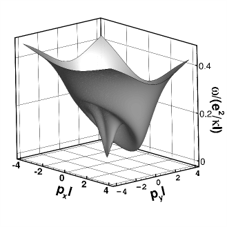
Figure 10: Dispersion relation in the orbital-coherent state at the Dzyaloshinskii-Moriya instability. Filling factor $\nu=-1$ and bias $\Delta_{B}=0.51$ $e^{2}/\kappa\ell.$

The eigenvector with positive frequency of Eq. (96) has

$$\frac{S_{x}}{S_{y}}=\frac{-J_{xy}-J_{yx}+i\sqrt{4J_{xx}J_{yy}-\left(J_{xy}+J_{yx}\right)^{2}}}{2J_{xx}}.$$ (111)

It follows, using Eq. (110), that, at the DM instability, the energy is lowered by forming coupled density-waves in $\hat{x}$ and $\hat{y}$ pseudospin components with:

$$\frac{S_{x}(\mathbf{q})}{S_{y}(\mathbf{q})}=-\frac{J_{xy}(\mathbf{q})}{J_{xx}(\mathbf{q})}=-\frac{J_{yy}(\mathbf{q})}{J_{xy}^{\ast}(\mathbf{q})}.$$ (112)

The real part of the $J_{xy}$ coupling, due mainly to the dipole electrostatic energy, is very small at the instability wavevector because the $N=0$ Landau level cannot support rapid spatial variation, as we have verified by explicit calculation. Because $J_{yy}(\mathbf{q})$ is real, it follows that $S_{x}$ and $S_{y}$ spatial variations are out of phase by nearly exactly $\pi/2$. If the magnitudes of the $S_{x}$ and $S_{y}$ components were identical, this would imply a spiral ground state. Because $J_{xx}(\mathbf{q})$ and $J_{yy}(\mathbf{q})$ are not identical at the instability, the spiral is somewhat distorted. It must be kept in mind, however, that the DM instability may be preempted by a first order transition to a state with lower energy and a more complex pseudospin pattern. A fuller exploration of the properties of these states, including their properties in the presence of an external electric field, is beyond the scope of the present work.

IX COLLECTIVE MODES IN THE MIXED STATE

The mixed state occurs between the inter-layer coherent and inter-orbital coherent phases as shown in Fig. 3. The width of this region in the phase diagram increases with magnetic field. In this phase, all order parameters $\left\langle\rho_{i,j}\right\rangle$ are finite so that this phase has both inter-layer and inter-orbital coherence. We show the behavior of some of these order parameters with bias in Fig. 4. The order parameters $\left\langle\rho_{1,4}\right\rangle$ and $\left\langle\rho_{2,3}\right\rangle$ which flip both valley and orbital indices are non zero in this phase.

The collective modes in the MS are obtained numerically by solving Eq. (54). The MS has three dispersive modes, as in the other two phases we studied. The dispersions of these modes differ from the dispersions in the other two phases at small wavevector only. We show in Fig. 11(a) the dispersion of the inter-orbital mode and in Fig. 11(b) the dispersion of the inter-layer coherent mode along the $x$ or $y$ axis and at $45^{\circ}$ ($xy$) from the $x$ axis. In contrast with the other two phases, both modes are now gapped for $\Delta_{B}$ not at the boundaries of this phase. As in the inter-orbital phase, the dispersions are highly anisotropic. We show in the next section that this phase has a distinct signature in the microwave absorption spectrum.

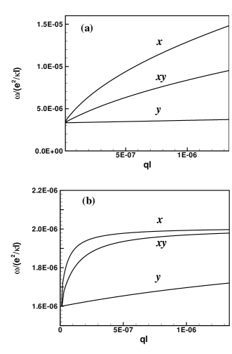
Figure 11: Dispersion relation of the (a) inter-orbital and (b) interlayer coherent modes in the mixed phase at $\Delta_{B}=0.00195$ $e^{2}/\kappa\ell$ and $B=10$ T along directions $x,y$ and $xy$ ($45^{\circ}$ from the $x$ axis).

X MICROWAVE ABSORPTION

The collective modes discussed in the previous sections can be detected in microwave absorption experiments, as we now show. We write the current operator, projected onto $N=0$ and valley $K$, as

$$j_{\xi K,i}=-c\left.\frac{\partial H_{\xi K}^{0}}{\partial A_{i}^{e}}\right|_{A_{i}^{e}=0},$$ (113)

where $A_{i}^{e}$ is the vector potential of the external electromagnetic field, $i=x,y$ and $H_{K}^{0}$ is given in Eq. (2). In second quantization, the total current is given by

$$\mathbf{J}_{\xi K}=\int d\mathbf{r}\Psi_{\xi K}^{{\dagger}}\left(\mathbf{r}\right)\mathbf{j}_{\xi K}\Psi_{\xi K}\left(\mathbf{r}\right),$$ (114)

with the field operators defined in Eqs. (20,26) and $\xi=\pm 1.$ We find that

$$\mathbf{J}_{\xi K}=\xi\sqrt{2}\beta\Delta_{B}\frac{e\ell}{\hslash}N_{\varphi}\left(\rho_{\xi K,y}\left(0\right)\widehat{\mathbf{x}}+\rho_{\xi K,x}\left(0\right)\widehat{\mathbf{y}}\right),$$ (115)

where

$$\rho_{K,x}\left(0\right) = \frac{1}{2}\left(\rho_{0,1}^{K,K}\left(0\right)+\rho_{1,0}^{K,K}\left(0\right)\right),$$ (116)

$$\rho_{K,y}\left(0\right) = \frac{1}{2i}\left(\rho_{0,1}^{K,K}\left(0\right)-\rho_{1,0}^{K,K}\left(0\right)\right),$$ (117)

and similarly for $\rho_{K^{\prime},x/y}\left(0\right).$ The same result for $\mathbf{J}_{\xi K}$ can be obtained by calculating the polarization current

$$\mathbf{J}_{\xi K}=\frac{d}{dt}\mathbf{d}_{\xi K}\left(\mathbf{q}\right),$$ (118)

with the dipole density $\mathbf{d}_{\xi K}\left(\mathbf{q}\right)$ defined in Eq. (VIII.1) and using the Heisenberg equation of motion $-i\hslash d/dt\left(\ldots\right)=\left[H_{\xi K}^{0},\left(\ldots\right)\right].$ We note that the orbitally coherent state has spontaneous currents in its ground state, a very exceptional property. It appears likely that, in finite systems, these currents should flow perpendicular to system boundaries, forcing domain structures in the pseudospin magnetization texture, consistent with expectations based on the electrostatic energy of the dipole density.

We define the total current-current correlation function Matsubara Green’s functions as

$$\chi_{J_{\alpha},J_{\beta}}\left(\tau\right) = -\frac{1}{S}\left\langle TJ_{\alpha}\left(\tau\right)J_{\beta}\left(0\right)\right\rangle$$

$$= \left(\frac{\Delta_{B}}{\gamma_{1}}\right)^{2}\frac{e^{2}\hslash^{2}}{4\pi m^{\ast 2}\ell^{4}}\sum_{i,j=K,K^{\prime}}\xi_{i}\xi_{j}\chi_{\rho_{i,\overline{\alpha}},\rho_{j,\overline{\beta}}}\left(\tau\right),$$

where $J_{\alpha}=J_{K,\alpha}+J_{K^{\prime},\alpha}$ and

$$\chi_{\rho_{i,\alpha},\rho_{j,\beta}}\left(\tau\right)=-\left\langle T\rho_{i,\alpha}\left(0,\tau\right)\rho_{j,\beta}\left(0,0\right)\right\rangle.$$ (120)

with $i,j=K,K^{\prime}$ and $\alpha,\beta=x,y.$ Note that $\overline{\alpha},\overline{\beta}$ are defined so that $\overline{x}=y,\overline{y}=x.$

The microwave absorption for an electric field oriented along the direction $\alpha$ is given by

$$P_{\alpha}\left(\omega\right) = -\frac{1}{\hslash}\Im\left[\frac{\chi_{J_{\alpha},J_{\alpha}}^{R}\left(\omega\right)}{\omega+i\delta}\right]E_{0}^{2}$$

$$= -\frac{1}{2}\left(\frac{e^{2}}{h}\right)\left(\frac{\Delta_{B}}{\gamma_{1}}\right)^{2}\omega_{c}^{\ast 2}$$

$$\times\sum_{i,j=K,K^{\prime}}\Im\left[\xi_{i}\xi_{j}\frac{\chi_{\rho_{i,\overline{\alpha},j,\overline{\alpha}}}^{R}\left(\omega\right)}{\omega+i\delta}\right]E_{0}^{2},$$

where we have assumed a uniform electric field $\mathbf{E}\left(t\right)=E_{0}\widehat{\mathbf{\alpha}}e^{-i\omega t}$ and taken the analytic continuation $i\Omega_{n}\rightarrow\omega+i\delta$ of $\chi_{J_{\alpha},J_{\alpha}}\left(0,\Omega_{n}\right)$ to get the retarded response function. The response functions $\chi_{\rho_{i\alpha}\rho_{j\alpha}}^{R}$ are calculated in units of $\hslash/\left(e^{2}/\kappa\ell\right)$ so that $P_{\alpha}\left(\omega\right)$ is the power absorbed per unit area. In Eq. (X) we have neglected a diamagnetic contribution to the current response which becomes important at low frequencies.

Our GRPA correlation functions are given by Eq. (54) and numerical results for the absorption in the inter-layer coherent phase are shown in Fig. 12. Exactly the same result is obtained, in this phase, if the electric field is set in the $y$ direction, i.e. the absorption is isotropic. We see that the signal in the absorption is at a frequency corresponding to the orbital-pseudospin mode (see Fig. 6). The frequency $\nu$ of this mode at $\mathbf{q}=0$ decreases with bias while the absorption intensity increases with bias. Since $e^{2}/\hbar\kappa\ell\sim 2.7\times 10^{3}\sqrt{B\left(\text{T}\right)}$ GHz (using $\kappa=5$ for graphene on SiO₂ substrate), the frequency of the orbital pseudospin mode at zero bias is $\nu\approx 3.4$ GHz $i.e.$ in the microwave regime. Note that mode $3$ in Fig. 5 is also present in the absorption at finite bias and that its frequency has a higher value outside of the microwave regime.

The absorption in the mixed state is shown in Fig. 13 on a logarithmic scale. The three lower peaks show the absorption from the inter-layer coherent mode which is gapped in the mixed state. The other three peaks are from the inter-orbital mode. The gaps in these two modes increase with bias until they reach a maximum around $\Delta_{B}=0.00195$ for $B=10$ T. The gaps then decreases with bias. The intensity of the absorption increases with bias for both modes. In Fig. 13, the electric field is set along the $y$ axis. The absorption is at least $100$ times lower if the electric field is oriented along the $x$ axis i.e. it is highly anisotropic in the mixed state. With our choice of phase for the ground state of the mixed state, the pseudospins (and so the electric dipoles according to Eq. (89)) are oriented in the $\widehat{\mathbf{y}}$ direction. Their motion for $q=0$ is an oscillation in the $x-y$ plane about the $y$ axis. For such a configuration, the electromagnetic absorption is strongest for fields along the $y$ axis, which is what we observe in our calculation.

In the orbital-coherent phase, the orbital-pseudospin mode is gapless and decoupled from the two other gapped modes. Since the orbital-coherent mode couples strongly to external electric fields, we can expect anomalous low-frequency absorption in this state, similar to the Drude absorption of a metal. This interesting and unusual absorption feature is likely to be highly sensitive to disorder. Its detailed analysis lies beyond the scope of the present paper. Above $\Delta_{B}^{\left(2\right)}$, the ground state has $\nu_{2}=\nu_{3}=\nu_{4}=1$ and there is no orbital coherence anymore. The OPM then has a gap that is proportional to $\Delta_{B}-\Delta_{B}^{\left(2\right)}.$ The OPM becomes visible in the absorption in this phase while the other modes do not.

In summary, we see that each of the three phases in the phase diagram at $\nu=-1$ has a different signature in the microwave absorption spectrum. We remark that the frequencies in Fig. 13 are quite small. But, they can be increased by increasing the magnetic field. For example, Fig. 14 shows the gap in the inter-layer and inter-orbital pseudospin modes in the three phases at a magnetic field of $40$ T.

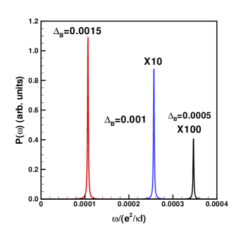
Figure 12: (Color online) Microwave absorption from the orbital pseudospin mode in the inter-layer phase at different values of the bias. The absorption is zero at zero bias. The second(third) peak has been multiplied by 10(100).

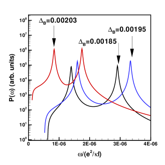
Figure 13: (Color online) Absorption spectrum in the mixed state at $B=10$ T for an electric field in the $y$ direction and for biases $\Delta_{B}=0.00185,0.00195,0.0020$ in units of $e^{2}/\kappa\ell$

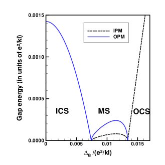
Figure 14: (Color online) Gaps in the inter-layer pseudospin mode (IPM) and in the orbital pseudospin mode (OPM) as a function of bias at $\nu=-1$ and $B=40$ T.

XI CONCLUSION

We have studied the phase diagram and collective excitations of a spin-polarized bilayer graphene 2DEG at filling factors $\nu=-1$ and $\nu=3$, as a function of a bias electric potential which shifts electrons between layers. Our study is based on the Hartree-Fock approximation for the mean-field ground state, and the GRPA for the collective modes and response functions.

We predict phase transitions between the following sequence of states with increasing potential bias: (1) an inter-layer-coherent state (ICS) with a zero gap inter-layer pseudospin mode (IPM) and an orbital pseudospin mode (OPM) with a small gap. This gap can be detected in microwave absorption experiment. Its frequency decreases with bias while its intensity increases with bias; (2) a mixed state (MS) with both inter-layer and inter-orbital coherence. Both the IPM and OPM are gapped and visible in microwaves in this phase. Moreover, the intensity of the absorption is highly sensitive to the direction of the external electric field; (3) an orbital coherent state (OCS) with orbital coherence concentrated in one layer only. (The second layer is completely filled.) The OCS state is a very simple one in which the low potential layer is filled and the high potential layer has a gap induced between it’s two Landau levels by spontaneously establishing coherence between states with $n=1$ and $n=0$ orbital character. This state has a number of quite unusual properties, including electric dipoles and associated uniform currents in its ground state. The OCS has a gapless (Goldstone) OPM and a gapped IPM. Both modes are absent from the absorption spectrum. The dispersions of the collective modes are also highly anisotropic in this phase. The phase is unstable at a finite wavevector due to the presence of a Dzyaloshinksii-Moriya exchange interaction. We believe that the instability will lead to the formation of a ground state with a non-uniform pseudosopin pattern.

These properties are associated with competition between an electron-electron interaction term which favors $n=0$ orbital occupation, and single-particle terms in the effective two-band model of Ref. mccann, which favors $n=1$ orbital occupation more strongly at larger inter-layer potential difference. We note that this band model neglect the $\gamma_{4}$ hopping term, which connects sites $A_{1}(B_{1})$ and $A_{2}(B_{2})$graphenereviews . Strictly speaking, the results obtained in our paper are valid if $\gamma_{4}=0.$ The effect of the $\gamma_{4}$ term is to add a negative correction to the energy of the $n=1$ orbital which is independent of the valley index, magnetic field and bias. More precisely: $E_{\mathbf{K,}n=1,X}=\frac{1}{2}\Delta_{B}-\beta\Delta_{B}+\zeta,E_{\mathbf{K}^{\prime},n=1,X}=-\frac{1}{2}\Delta_{B}+\beta\Delta_{B}+\zeta$ with $\zeta=\sqrt{6\beta}\gamma_{4}a_{0}/\ell.$ It is not clear from the literature what is the precise value of the $\gamma_{4}$ parameter. In Ref. peeters, , the value $\gamma_{4}=-0.12$ is obtained by comparing the tight-binding model for bilayer graphene with the Slonczewski-Weiss-McClure tight-binding model for bulk graphitemcclure . In bulk graphite, $\gamma_{4}\approx 0.044$ eV. With $\gamma_{4}=-0.12$, the correction $\zeta<\Delta_{B}$ for $\Delta_{B}>0.02$ $e^{2}/\kappa\ell.$ It follows that this term may have an effect on the existence of the interlayer coherent and mixed phases, and certainly on the location of their phase boundaries, $\Delta_{B,num}^{(3)}$ and $\Delta_{B}^{(1)}$, since level $n=1$ may be below level $n=0$ in both layers. The Dzyaloshinksii-Moriya transition, however, occurs at a large bias of $\Delta_{B}\approx 0.5$ $e^{2}/\kappa\ell$ in a region where the single-particle energy of level $n=1$ is already well below that of level $n=0.$ For this reason we believe that the physics in this region should not be affected by $\gamma_{4}.$ More numerical work is needed, however, to assess the precise influence of this term.

Appendix A HARTREE AND FOCK INTERACTIONS

We first give the definitions of the Hartree, $H,$ and Fock, $X,$ interactions in Eqs. (30,31,32,33):

$$h_{1}\left(q\right) = H_{0,0,0,0}\left(q\right)=\frac{1}{q\ell}\Lambda\left(q\right),$$ (122)

$$h_{2}\left(\mathbf{q}\right) = H_{0,0,0,1}\left(\mathbf{q}\right)=-\frac{i}{\sqrt{2}}e^{i\theta_{\mathbf{q}}}\Lambda\left(q\right),$$ (123)

$$h_{4}\left(q\right) = H_{0,0,1,1}\left(q\right)=\frac{1}{q\ell}\left(1-\frac{q^{2}\ell^{2}}{2}\right)\Lambda\left(q\right),$$ (124)

$$h_{6}\left(\mathbf{q}\right) = H_{0,1,0,1}\left(\mathbf{q}\right)=\frac{1}{2}q\ell e^{2i\theta_{\mathbf{q}}}\Lambda\left(q\right),$$ (125)

$$h_{7}\left(q\right) = H_{0,1,1,0}\left(q\right)=\frac{1}{2}q\ell\Lambda\left(q\right),$$ (126)

$$h_{8}\left(\mathbf{q}\right) = H_{0,1,1,1}\left(\mathbf{q}\right)=\frac{i}{\sqrt{2}}e^{i\theta_{\mathbf{q}}}$$

$$\times\left(1-\frac{q^{2}\ell^{2}}{2}\right)\Lambda\left(q\right),$$

$$h_{16}\left(q\right) = H_{1,1,1,1}\left(q\right)=\frac{1}{q\ell}\left(1-\frac{q^{2}\ell^{2}}{2}\right)\Lambda\left(q\right)$$ (128)

and

$$h_{3} = H_{0,0,1,0}\left(\mathbf{q}\right)=-h_{2}^{\ast},$$ (129)

$$h_{5} = H_{0,1,0,0}\left(\mathbf{q}\right)=-h_{2},$$ (130)

$$h_{9} = H_{1,0,0,0}\left(\mathbf{q}\right)=h_{2}^{\ast},$$ (131)

$$h_{10} = H_{1,0,0,1}\left(q\right)=h_{7},$$ (132)

$$h_{11} = H_{1,0,1,0}\left(\mathbf{q}\right)=h_{6}^{\ast},$$ (133)

$$h_{12} = H_{1,0,1,1}\left(\mathbf{q}\right)=-h_{8}^{\ast},$$ (134)

$$h_{13} = H_{1,1,0,0}\left(q\right)=h_{4},$$ (135)

$$h_{14} = H_{1,1,0,1}\left(\mathbf{q}\right)=-h_{8},$$ (136)

$$h_{15} = H_{1,1,1,0}\left(\mathbf{q}\right)=h_{8}^{\ast},$$ (137)

where $\theta_{\mathbf{q}}$ is the angle between the wavevector $\mathbf{q}$ and the $x$ axis and $\Lambda\left(q\right)=\exp\left(\frac{-q^{2}\ell^{2}}{2}\right).$ The interactions $\widetilde{h}_{n}\left(\mathbf{q}\right)$ are obtained by multiplying $h_{n}$ by $e^{-qd}$ where $d$ is the inter-layer separation. The interactions $\widehat{h}_{n}\left(\mathbf{q}\right)$ and $\widehat{\widetilde{h}}_{n}$ are obtained by removing the term $i$ and the phase factor $e^{\pm i\theta_{\mathbf{q}}}$ or $e^{\pm 2i\theta_{\mathbf{q}}}$ in $h_{n}$ and $\widetilde{h}_{n}$. For example $\widehat{h}_{2}=-\Lambda\left(q\right)/\sqrt{2}$ while $h_{2}\left(\mathbf{q}\right)=-\frac{i}{\sqrt{2}}e^{i\theta_{\mathbf{q}}}\Lambda\left(q\right).$

The Fock interactions are defined by

$$x_{1}\left(q\right)=X_{0,0,0,0}\left(\mathbf{q}\right)=\int_{0}^{\infty}dye^{-y^{2}/2}J_{0}\left(q\ell y\right),$$ (138)

$$x_{2}\left(\mathbf{q}\right)=X_{0,0,0,1}\left(\mathbf{q}\right)=\frac{i}{\sqrt{2}}e^{i\theta_{\mathbf{q}}}\int_{0}^{\infty}dyye^{-y^{2}/2}J_{1}\left(q\ell y\right),$$ (139)

$$x_{4}\left(q\right)=X_{0,0,1,1}\left(\mathbf{q}\right)=\int_{0}^{\infty}dy\left(1-\frac{y^{2}}{2}\right)e^{-y^{2}/2}J_{0}\left(q\ell y\right),$$ (140)

$$x_{6}\left(\mathbf{q}\right)=X_{0,1,0,1}\left(\mathbf{q}\right)=\frac{1}{2}e^{2i\theta_{\mathbf{q}}}\int_{0}^{\infty}dyy^{2}e^{-y^{2}/2}J_{2}\left(q\ell y\right),$$ (141)

$$x_{7}\left(q\right)=X_{0,1,1,0}\left(\mathbf{q}\right)=\frac{1}{2}\int_{0}^{\infty}dyy^{2}e^{-y^{2}/2}J_{0}\left(q\ell y\right),$$ (142)

$$x_{8}\left(\mathbf{q}\right) = X_{0,1,1,1}\left(\mathbf{q}\right)=-\frac{i}{\sqrt{2}}e^{i\theta_{\mathbf{q}}}\int_{0}^{\infty}dyy$$

$$\times\left(1-\frac{y^{2}}{2}\right)e^{-y^{2}/2}J_{1}\left(q\ell y\right),$$

$$x_{16}\left(q\right)=X_{1,1,1,1}\left(\mathbf{q}\right)=\int_{0}^{\infty}dy\left(1-\frac{y^{2}}{2}\right)^{2}e^{-y^{2}/2}J_{0}\left(q\ell y\right),$$ (144)

and

$$x_{3} = X_{0,0,1,0}\left(\mathbf{q}\right)=x_{2}^{\ast},$$ (145)

$$x_{5} = X_{0,1,0,0}\left(\mathbf{q}\right)=-x_{2,}$$ (146)

$$x_{9} = X_{1,0,0,0}\left(\mathbf{q}\right)=-x_{2}^{\ast},$$ (147)

$$x_{10} = X_{1,0,0,1}\left(q\right)=x_{7},$$ (148)

$$x_{11} = X_{1,0,1,0}\left(\mathbf{q}\right)=x_{6}^{\ast},$$ (149)

$$x_{12} = X_{1,0,1,1}\left(\mathbf{q}\right)=x_{8}^{\ast},$$ (150)

$$x_{13} = X_{1,1,0,0}\left(q\right)=x_{4},$$ (151)

$$x_{14} = X_{1,1,0,1}\left(\mathbf{q}\right)=-x_{8},$$ (152)

$$x_{15} = X_{1,1,1,0}\left(\mathbf{q}\right)=-x_{8}^{\ast}.$$ (153)

The interactions $\widetilde{x}_{n}$ are obtained by multiplying the integrand by $e^{-yd/\ell}$. The interactions $\widehat{x}_{n}$ and $\widehat{\widetilde{x}}_{n}$ are obtained by removing the imaginary term $i$ and the phase factor.

The combinations:

$$H_{i} = h_{i}-\widetilde{h}_{i},$$ (154)

$$T_{i} = h_{i}+\widetilde{h}_{i},$$ (155)

$$X_{i} = x_{i}+\widetilde{x}_{i},$$ (156)

$$U_{i} = x_{i}-\widetilde{x}_{i}.$$ (157)

To define $\widehat{H}_{n},\widehat{T}_{n},\widehat{X}_{n},\widehat{U}_{n},$ we follow the same procedure as for $\widehat{h}_{n},\widehat{\widetilde{h}}_{n},\widehat{x}_{n},\widehat{\widetilde{x}}_{n}.$

Some useful constants:

$$x_{1}\left(0\right)=\sqrt{\frac{\pi}{2}},$$ (158)

$$x_{4}\left(0\right)=\frac{1}{2}\sqrt{\frac{\pi}{2}},$$ (159)

$$x_{7}\left(0\right)=\frac{1}{2}\sqrt{\frac{\pi}{2}},$$ (160)

$$x_{16}\left(0\right)=\frac{3}{4}\sqrt{\frac{\pi}{2}}.$$ (161)

Appendix B MATRIX $F_{1}$ FOR THE INTER-LAYER-COHERENT MODES

The collective modes at $\nu=-1$ and $\Delta_{B}<\Delta_{B}^{(1)}$ involve the matrices $F_{1}\left(q\right)$ in Eq. (72). The elements of this matrix are defined by

$$A\left(q\right) = \widetilde{x}_{4}\left(0\right)-\widetilde{x}_{1}\left(0\right)-\frac{3}{4}x_{1}\left(0\right)-\widetilde{x}_{16}\left(0\right)$$

$$+X_{4}\left(q\right)-H_{1}\left(q\right)+H_{4}\left(q\right),$$

$$B\left(q\right) = 2\Delta_{B}^{c}\left(\beta-1\right)+H_{1}\left(q\right)-H_{4}\left(q\right)-U_{4}\left(q\right)$$

$$+\widetilde{x}_{1}\left(0\right)-\frac{5}{4}x_{1}\left(0\right)-\widetilde{x}_{4}\left(0\right)+\widetilde{x}_{16}\left(0\right)+2\frac{d}{\ell},$$

$$C\left(q\right)=-H_{16}\left(q\right)+X_{16}\left(q\right)-2\widetilde{x}_{16}\left(0\right),$$ (164)

$$D\left(q\right) = 2\Delta_{B}^{c}\left(2\beta-1\right)+H_{16}\left(q\right)-U_{16}\left(q\right)$$

$$+2\widetilde{x}_{16}\left(0\right)-\frac{3}{2}x_{1}\left(0\right)+2\frac{d}{\ell},$$

$$E\left(q\right) = T_{4}\left(q\right)+X_{4}\left(q\right)-T_{1}\left(q\right)+\widetilde{x}_{1}\left(0\right)$$

$$-\widetilde{x}_{4}\left(0\right)-\frac{3}{4}x_{1}\left(0\right)-\widetilde{x}_{16}\left(0\right),$$

$$F\left(q\right) = 2\beta\Delta_{B}^{c}-H_{1}\left(q\right)+H_{4}\left(q\right)+U_{4}\left(q\right)$$

$$+\widetilde{x}_{4}\left(0\right)-\widetilde{x}_{1}\left(0\right)-\frac{1}{4}x_{1}\left(0\right)+\widetilde{x}_{16}\left(0\right),$$

$$G\left(q\right) = \Delta_{B}^{c}-H_{1}\left(q\right)+H_{4}\left(q\right)+U_{4}\left(q\right)$$

$$+\widetilde{x}_{4}\left(0\right)-\widetilde{x}_{1}\left(0\right)+\frac{1}{2}x_{1}\left(0\right)-\frac{d}{\ell},$$

$$H\left(q\right)=\widehat{H}_{6}\left(q\right)-\widehat{U}_{6}\left(q\right),$$ (169)

$$J\left(q\right)=\widehat{H}_{8}\left(q\right)-\widehat{U}_{8}\left(q\right),$$ (170)

$$K\left(q\right)=\widehat{X}_{6}\left(q\right)-\widehat{T}_{6}\left(q\right),$$ (171)

$$M\left(q\right)=H_{16}\left(q\right)-U_{16}\left(q\right),$$ (172)

$$N\left(q\right)=\widehat{H}_{8}\left(q\right)-\widehat{X}_{8}\left(q\right).$$ (173)

To get the gap given by Eq. (80), we use

$$\left|E\left(0\right)\right| = \left|-\frac{1}{4}\sqrt{\frac{\pi}{2}}+\widetilde{x}_{1}\left(0\right)-\widetilde{x}_{16}\left(0\right)\right|$$ (174)

$$= x_{1}\left(0\right)-\widetilde{x}_{1}\left(0\right)-x_{16}\left(0\right)+\widetilde{x}_{16}\left(0\right),$$

$$K\left(0\right) = 0.$$ (175)

Appendix C EXCHANGE ENERGY PSEUDOSPIN DEPENDENCE

It is possible to derive a rather general and instructive expression for the exchange energy of a pseudospin-$1/2$ quantum Hall ferromagnet, for the case in which the pseudospin texture varies in one direction only. In the following we take this direction to be the $\hat{x}$ direction and choose a Landau gauge in which the guiding centers orbits are localized as a function of this coordinate. If we are interested only in the dependence of energy on pseusospin texture we can assume that every guiding center orbital is occupied by one electron, but leave the pseudospin of that orbital arbitrary. It is not necessary to immediately specify the orbital character of the states that form the pseudospin and we refer to them for the moment as state A and state B. In the case of immediate interest in this paper, state A has $n=0$ orbital character and state B has $n=1$ orbital character. We discuss some other examples below.

The pseudospin texture can be specified by the two-component pseudospinors at each guiding center,

$$|\Psi_{X}\rangle=\left(\begin{array}[]{c}z_{X}^{A}\\ z_{X}^{B}\end{array}\right),$$ (176)

or by the guiding center dependent direction cosines of the pseudospin orientation: $(n_{X}^{x},n_{X}^{y},n_{X}^{z})=(\sin(\theta_{X})\cos(\phi_{X}),\sin(\theta_{X})\sin(\phi_{X}),\cos(\theta_{X}))$ where $\theta_{X}$ and $\phi_{X}$ are the pseudospin orientation polar and azimuthal angles. When a specific gauge choice is convenient we use $z^{A}=\cos(\theta/2)$ and $z^{B}=\sin(\theta/2)\exp(i\phi)$.

The exchange energy of a pseudospin quantum Hall ferromagnet is

$$E_{x}=-\frac{1}{2}\sum_{X,X^{\prime}}\;\langle X,X^{\prime}|V_{ee}|X^{\prime},X\rangle.$$ (177)

The dependence of exchange energy on pseudospin texture can be exhibited explicitly by using the property that each $\exp(i\mathbf{k\cdot(r_{1}-r_{2})})$ term in the Fourier expansion of the two-particle interaction matrix elements can be separated into factors that depend on ${\mathbf{r}_{1}}$ and ${\mathbf{r}_{2}}$ independently. It follows that

$$E_{x}=-\frac{1}{2}\sum_{X,X^{\prime}}\;n_{X^{\prime}}^{\alpha}\,J_{X^{\prime},X}^{\alpha,\beta}\,n_{X}^{\beta}$$ (178)

where the Greek indices $\alpha=c,x,y,z$, $n^{c}\equiv 1$ represents the filling factor of the guiding center states,

$$J_{X^{\prime},X}^{\alpha,\beta}=\frac{1}{A}\sum_{\mathbf{q}}\exp(-q^{2}\ell^{2}/2)\;f^{\alpha,\beta}({\mathbf{q}})\;V(\mathbf{q})\;\delta_{X^{\prime}-X,\ell^{2}q_{y}},$$ (179)

$\ell$ is the magnetic length, $V(\mathbf{q})$ is the Fourier-transform of the electron-electron interaction and $f^{\alpha,\beta}({\mathbf{q}})$ is an interaction form factor. Eq. (179) follows from the following expression for the plane-wave matrix elements:

$$\langle X^{\prime}|\exp(i\mathbf{q\cdot r})|X\rangle = \delta_{X^{\prime},X+\ell^{2}q_{y}}\exp(-q^{2}\ell^{2}/4)$$ (180)

$$\times \sum_{I^{\prime},I}\;{\bar{z}}_{X^{\prime}}^{I^{\prime}}\,F^{I^{\prime},I}({\mathbf{q}})\,z_{X}^{I},$$

where the overbar accent denotes complex conjugation. The character of the cyclotron orbitals in the two nearly degenerate Landau levels is captured by the single-particle form factors $F^{I^{\prime},I}({\mathbf{q}})$. For example if pseudospin $I$ has orbital Landau level index $n_{I}$, $F^{I^{\prime},I}({\mathbf{q}})=F_{n_{I^{\prime}},n_{I}}({\mathbf{q}})$ where $F_{n^{\prime},n}({\mathbf{q}})$ is the familiar two-dimensional electron gas Landau-level form factorleshouches , commonly used in the analysis of many-different properties in the quantum Hall regime. Note that $F^{I^{\prime},I}(\mathbf{q})={\bar{F}}^{I,I^{\prime}}(\mathbf{-q})$ For the example of quantum Hall ferromagnetism discussed in this paper, $n_{A}=0$ and $n_{B}=1$ when the bias potential is strong enough to yield complete layer polarization. (The analysis in this section does not apply when both orbital and layer degrees of freedom are in play.) When the $A$ and $B$ orbitals have opposite spins, a common occurrence in quantum Hall ferromagnetism, $F^{A,B}({\mathbf{q}})\equiv 0$. Examples in which the $A$ and $B$ orbitals are centered in different two-dimensional layers require a slight generalization of the present discussion which we do not explicitly address.

Using Eq. (180) we find (leaving the wavevector dependence of the single-particle and interaction form factors implicit) that

$$4f^{0,0} = |F^{A,A}|^{2}+|F^{B,B}|^{2}+|F^{A,B}|^{2}+|F^{B,A}|^{2}$$

$$4f^{0,x} = 2\mathrm{Re}[\bar{F}^{A,A}F^{A,B}+\bar{F}^{B,A}F^{B,B}]$$

$$4f^{0,y} = -2\mathrm{Im}[\bar{F}^{A,A}F^{A,B}+\bar{F}^{B,A}F^{B,B}]$$

$$4f^{0,z} = |F^{A,A}|^{2}-|F^{B,B}|^{2}-|F^{A,B}|^{2}+|F^{B,A}|^{2}$$

$$4f^{x,x} = 2\mathrm{Re}[F^{A,A}\bar{F}^{B,B}+F^{B,A}\bar{F}^{A,B}]$$

$$4f^{y,y} = 2\mathrm{Re}[F^{A,A}\bar{F}^{B,B}-F^{B,A}\bar{F}^{A,B}]$$

$$4f^{z,z} = |F^{A,A}|^{2}+|F^{B,B}|^{2}-|F^{A,B}|^{2}-|F^{B,A}|^{2}$$

$$4f^{x,y} = 2\mathrm{Im}[F^{A,A}\bar{F}^{B,B}+F^{B,A}\bar{F}^{A,B}]$$

$$4f^{x,z} = 2\mathrm{Re}[F^{A,A}\bar{F}^{B,A}-\bar{F}^{B,B}F^{A,B}]$$

$$4f^{y,z} = -2\mathrm{Im}[F^{A,A}\bar{F}^{B,A}-\bar{F}^{B,B}F^{A,B}].$$ (181)

These results are obtained after replacing the pseudospinors by pseudospin direction cosines using

$$2\bar{z}^{A}z^{A} = 1+n^{z}$$

$$2\bar{z}^{B}z^{B} = 1-n^{z}$$

$$2\bar{z}^{A}z^{B} = n^{x}+in^{y}$$ (182)

Note that because the exchange energy is real, all the interaction form factors are real. The diagonal interaction form factors are even functions of $\mathbf{q}$, while the off-diagonal form factors have both even and odd contributions. The interaction form factors capture the influence of the shape of the pseudospin state dependent cyclotron orbits on exchange energies. In the limit $\mathbf{q}\rightarrow 0$, orthogonality implies that $F^{A,B}\rightarrow\delta_{A,B}$. If follows that $f^{\alpha,\beta}(\mathbf{q}=0)=\delta_{\alpha,\beta}/2$.

The exchange energy expression can be written in an alternate form by Fourier transforming along the direction perpendicular to the guiding center orbitals, defining

$$n_{p}^{\alpha}=\frac{1}{N_{\phi}}\,\sum_{X}\,\exp(-ipX)\,n_{X}^{\alpha}$$ (183)

where $N_{\phi}=2\pi\ell^{2}/A$ is the number of guiding center orbitals in a Landau level. The exchange energy then takes a form from which spin-wave dispersions can be simply read off:

$$E_{x}=-\frac{1}{2}\sum_{p}{\bar{n}}_{p}^{\alpha}\,J_{p}^{\alpha,\beta}\,n_{p}^{\beta}$$ (184)

with the momentum space exchange integral given by

$$J_{p}^{\alpha,\beta}=\int\frac{d^{2}\mathbf{q}}{(2\pi)^{2}}\,\exp(-ipq_{y}\ell^{2})\,\exp(-q^{2}\ell^{2}/2)\,f^{\alpha,\beta}(\mathbf{q})\;V(\mathbf{q}).$$ (185)

Because $f^{\alpha,\beta}$ is real, $J_{-p}^{\alpha,\beta}={\bar{J}}_{p}^{\alpha,\beta}$. Similarly, for the diagonal elements of $J$, the property that the diagonal elements of $f$ are even functions of $\mathbf{q}$ implies that $J_{p}^{\alpha,\beta}=J_{-p}^{\alpha,\beta}$. Combining both properties, we conclude that the diagonal momentum space interactions are real. The off-diagonal elements, however, can have both even real and odd imaginary contributions. For $p\ell\gg 1$, the integration over $\mathbf{q}$ in Eq. (185) has contributions from small $\mathbf{q}$ only, allowing us to set $\exp(-q^{2}\ell^{2}/2)\,f^{\alpha,\beta}(\mathbf{q})\rightarrow\delta_{\alpha,\beta}/2$. The integral can then be recognized as an inverse Fourier transform of the electron-electron interaction from momentum space back to real space. It follows that,

$$J_{p\rightarrow\infty}^{\alpha,\beta}=\frac{\delta_{\alpha,\beta}e^{2}}{2\epsilon|p|\ell^{2}}.$$ (186)

This is the familiar peculiarity of quantum Hall systems in which exchange interactions at large momenta are most simply understoodKallinHalperin after a particle hole transformation which converts them into Hartree interactions between electrons and holes. In strong fields the particle and hole in a magnetoexciton with momentum $p$ are separated in real space by $p\ell^{2}$. For very large $p$, the separation between particle and hole is larger than the cyclotron orbit sizes and the interaction is approximately given by the interaction between point charges. For smaller values of $p$ the size and shape of the cyclotron orbit, represented in momentum space by $\exp(-q^{2}\ell^{2}/2)\,f^{\alpha,\beta}(\mathbf{q})$ becomes important.

Imaginary off-diagonal contributions to $J_{p}^{\alpha,\beta}$ are responsible for DM-like interactions in quantum Hall ferromagnets. In the example discussed in this paper for instance, the $A$ orbital has orbital Landau level index $n=0$, while the $B$ orbital has the same spin and $n=1$. It follows that $F^{A,A}=L_{0}(q^{2}\ell^{2}/2)$ and $F^{B,B}=L_{1}(q^{2}\ell^{2}/2)$ , where $L_{n}$ is a Laguerre polynomial, and that $F^{B,A}=iq\ell\exp(i\theta_{\mathbf{q}})/\sqrt{2}$ where $\theta_{\mathbf{q}}$ is the orientation angle of $\mathbf{q}$. It follows that $f^{x,y}$ vanishes. The generalized random-phase-approximation that we use in the main text for collective mode calculations is equivalent to linearized pseudospin-wave theory. For fluctuations around a ground state with pseudospin orientation polar angle $\theta_{B}$ (as discussed in the main text), the $J_{p}^{x,z}$ and $J_{p}^{y,z}$ pseudospin interactions give rise to DM-like interactions whose strength is proportional to $\sin(\theta_{B})$. The DM interactions can be viewed in particle-hole language as a consequence of the property that the interaction between an electron with pseudospin in the $\hat{x}-\hat{y}$ plane at $X$ and a hole with pseudospin in the $\hat{z}$ direction at $X^{\prime}$ is not invariant under the interchange of $X$ and $X^{\prime}$. This property reflects the pseudospin dependence of dipole and other higher order multipoles in the cyclotron orbit cloud of an electron with a particular pseudospin.

The analysis presented in this section, can be applied to any quantum Hall ferromagnet. One elementary example is the case where the pseudospin orbitals share Landau level index $n$ and have opposite spins. In this case

$$f^{\alpha,\beta}\to\frac{\delta_{\alpha,\beta}(L_{n}(q^{2}\ell^{2}/2))}{2}.$$ (187)

The pseudospin model has isotropic Heisenberg interactions and the pseudospin-wave excitation energy expression $\omega_{p}=2(J_{p=0}-J_{p})$, follows immediately from an expansion of the exchange energy function to quadratic order.