Anomalous thermal properties of a harmonic chain with correlated isotopic disorder

Abstract

We analyse the thermal properties of a harmonic chain with weak correlated disorder. With the use of a perturbative approach we derive analytical expressions for the time-evolution of the chain temperature and of the heat flow when both ends of the chain are coupled to heat baths. Our analytical and numerical results demonstrate that specific long-range correlations of the isotopic disorder can suppress or enhance the vibrational modes in pre-defined frequency windows. In this way one can arrange a frequency-selective heat flow through disordered chains.

Pacs: 44.10.+i, 63.50.Gh, 63.20.Pw

1 Introduction

One-dimensional (1D) harmonic chains constitute convenient models for the effective study of thermal transport in solids. On the one hand, they represent one of the few cases for which analytical results can be obtained with a relative ease. On the other hand, they can be used to describe the features of solids in the low-temperature region, where nonlinear effects can be neglected. For these reasons the heat conduction in 1D harmonic chains has long been a subject of active investigation (see [1, 2] and references therein).

This paper is devoted to the study of the thermal properties of 1D harmonic chains with correlated isotopic disorder. Since the mid-1990s the interest in models of this kind has been constantly increasing [3], especially after it became clear that specific long-range correlations in random potentials can create a sort of delocalisation transition even in 1D models [4, 5]. In the past ten years many studies, both at the theoretical [6, 7, 8] and experimental [9, 10] level, have thrown light on the phenomenon of enhancement or suppression of the Anderson localisation in low-dimensional systems with correlated random potentials. Within the field of 1D models with correlated disorder, some recent studies have begun to analyse the chains with long-range correlated random masses. These early works were focused on the anomalous diffusion of an initially localised energy input [11], or on the structure of the eigenmodes and on the statistics of the vibrational spectrum [12].

The present work adopts a different perspective, considering harmonic chains as open systems weakly coupled at both ends to Langevin heat baths as in the Casher-Lebowitz model [13]. The purpose of our study is twofold: to analyse the approach to the steady-state regime of the chain and to discuss the effects of long-range correlations of the isotopic disorder on the heat conduction. Accordingly, we first analyse the dynamics of 1D harmonic chains with random masses, without specifying the statistical properties of the disorder. Using standard tools of stochastic calculus, we obtain analytical expressions for the temperature profile and heat flux, describing the evolution of the system toward the steady-state regime. In the stationary limit, our expressions reduce to the formulae first obtained by Matsuda and Ishii [14] and Lebowitz and coworkers [13].

After, we focus on the thermal effects of long-range correletions. In a homogeneous chain all vibrational modes are extended, whereas in a random chain with uncorrelated disorder only low-frequency modes are significantly non-localised. However, specific long-range correlations of the disorder can generate the delocalisation or enhanced localisation of vibrational modes in predefined frequency windows. Thus, with an appropriate selection of the frequency intervals one can create a random chain with a finite fraction of extended modes in the middle of the frequency spectrum. This allows one to have a random chain with specific properties of thermal transport peculiar to models that are neither completely random nor perfectly ordered.

As an example, we show how to construct a random chain whose conductivity tends to scale with the size of the system regardless of the boundary conditions. We also demonstrate that with a proper choice of long-range correlations one can enhance the localisation of the eigenmodes within a wide range of the frequency spectrum. In this way one can reduce the thermal conductivity of the chain with respect to that of a chain with white-noise disorder.

2 The temperature profile and heat flux

We consider a harmonic chain of $N$ masses $m_{1},\ldots,m_{N}$ and we study its dynamics when the chain is weakly coupled to two Langevin baths at temperatures $T_{+}$ and $T_{-}$. The time evolution is described by the system of stochastic Itô equations

$$\begin{array}[]{ccl}dq_{i}&=&\displaystyle\frac{p_{i}}{m_{i}}dt\\ dp_{i}&=&\displaystyle\left[\sum_{j}{\bf D}_{ij}q_{j}-\delta_{i1}\frac{\lambda}{m_{1}}p_{1}-\delta_{iN}\frac{\lambda}{m_{N}}p_{N}\right]dt\\ &+&\displaystyle\delta_{i1}\sqrt{2\lambda k_{B}T_{-}}\,dW_{-}+\delta_{iN}\sqrt{2\lambda k_{B}T_{+}}\,dW_{+}\\ \end{array}$$ (1)

with $i=1,\ldots,N$. In eq. (1), $p_{i}$ and $q_{i}$ represent the momentum and the displacement from the equilibrium position of the $i$-th mass of the chain. The symbols $W_{+}(t)$ and $W_{-}(t)$ stand for two independent Wiener processes, while $\lambda$ represents the coupling constant of the chain to the baths. Finally, ${\bf D}$ is the tridiagonal force-constant matrix, with elements ${\bf D}_{ij}=2k\delta_{i,j}-k\delta_{i,j-1}-k\delta_{i,j+1}$ for $i=2,\ldots,N-1$ and $j=1,\ldots,N$ while the first and last rows take different forms according to the chosen boundary conditions. For fixed boundary conditions one has ${\bf D}_{1,j}=2k\delta_{1,j}-k\delta_{1,j-1}$ and ${\bf D}_{N,j}=2k\delta_{N,j}-k\delta_{N,j+1}$, while for free boundary conditions the matrix elements are ${\bf D}_{1,j}=k\delta_{1,j}-k\delta_{1,j-1}$ and ${\bf D}_{N,j}=k\delta_{N,j}-k\delta_{N,j+1}$.

To analyse the dynamics of the chain it is convenient to switch to normal coordinates and momenta, defined by the equations

$$\begin{array}[]{ccc}\displaystyle Q_{i}=\sum_{k=1}^{N}e_{k}^{(i)}\sqrt{m_{k}}q_{k},&&\displaystyle P_{i}=\sum_{k=1}^{N}e_{k}^{(i)}p_{k}/\sqrt{m_{k}}.\end{array}$$ (2)

Here $e_{k}^{(i)}$ is the $k$-th component of the $i$-th eigenvector of the rescaled force-constant matrix

$${\bf\tilde{D}}=\left({\bf M}^{-1/2}\right)^{\rm T}{\bf D}{\bf M}^{-1/2}$$ (3)

with eigenvalue $\omega_{i}^{2}$, i.e., ${\bf\tilde{D}}e^{(i)}=\omega_{i}^{2}e^{(i)}$ . In eq. (3), the symbol ${\bf M}$ stands for the mass matrix ${\bf M}_{ij}=m_{i}\delta_{ij}$ . As can be seen from eq. (2), the $k$-th component of the $i$-th vector $e^{(i)}$ defines the amplitude of the oscillations of the $k$-th mass in the $i$-th normal mode. For this reason we will refer to the vectors $e^{(i)}$ as displacement eigenvectors.

After passing to the normal coordinates, the dynamical equations of the chain can be written in a compact form by introducing the $2N$-component vector ${\bf X}=(Q_{1},\ldots,Q_{N},P_{1},\ldots,P_{N})$ and the $2N\times 2N$ matrix

$${\bf A}_{ij}=\delta_{i,j-N}-\omega_{j}^{2}\delta_{i-N,j}-\lambda{\bf C}_{i-N,j-N},$$ (4)

with the coupling matrix ${\bf C}$ being defined by

$${\bf C}_{ij}=\left\{\begin{array}[]{ccl}\displaystyle\frac{e_{1}^{(i)}e_{1}^{(j)}}{m_{1}}+\frac{e_{N}^{(i)}e_{N}^{(j)}}{m_{N}}&&\mbox{ if }i,j=1,\ldots,N\\ 0&&\mbox{ otherwise}\\ \end{array}.\right.$$ (5)

We also need to introduce the $2N\times 2$ matrix

$${\bf B}=\left(\begin{array}[]{cc}0&0\\ \vdots&\vdots\\ 0&0\\ \sqrt{2\lambda k_{B}T_{-}/m_{1}}e_{1}^{(1)}&\sqrt{2\lambda k_{B}T_{+}/m_{N}}e_{N}^{(1)}\\ \vdots&\vdots\\ \sqrt{2\lambda k_{B}T_{-}/m_{1}}e_{1}^{(N)}&\sqrt{2\lambda k_{B}T_{+}/m_{N}}e_{N}^{(N)}\\ \end{array}\right)$$ (6)

and the two-component Wiener process ${\bf W}(t)=\left(W_{-}(t),W_{+}(t)\right)$. Then one can write the dynamical equation in the form

$$d{\bf X}={\bf A}{\bf X}\;dt+{\bf B}\;d{\bf W}.$$ (7)

Eqs. (4) and (7) show that the interaction of the chain with the bath couples the normal modes, which are not independent as would be the case for an autonomous chain. From eq. (6) one should also notice that the coupling of each normal mode to the baths is proportional to to the first and the $N$-th components of the corresponding displacement vector.

Given the deterministic initial condition ${\bf X}(0)={\bf X}_{0}$, the formal solution of the stochastic equation (7) can be expressed in the form

$${\bf X}(t)={\bf U}(t)\left[{\bf X}_{0}+\int_{0}^{\infty}{\bf U}(-\tau){\bf B}\,d{\bf W}(\tau)\right],$$ (8)

where ${\bf U}(t)=\exp\left({\bf A}t\right)$ is the fundamental matrix of eq. (7). Eq. (8) defines a stochastic process which is Markovian, Gaussian, and that becomes stationary over sufficiently long time-scales provided that the eigenvalues of the matrix ${\bf A}$ have negative real parts [15]. In other words, the stochastic process (8) is a Ornstein-Uhlenbeck process in the broad sense. The Gaussian character of the process implies that its statistical properties are completely determined once the first two moments are known. One can easily show that the average value has the form ${\bf m}(t)=\langle{\bf X}(t)\rangle={\bf U}(t){\bf X}_{0}$ , while the covariance matrix can be expressed as

$$\begin{array}[]{ccl}{\bf K}_{ij}(t)&=&\displaystyle\langle\left({\bf X}_{i}(t)-{\bf m}_{i}(t)\right)\left({\bf X}_{j}(t)-{\bf m}_{j}(t)\right)\rangle\\ &=&\displaystyle\int_{0}^{t}\left[{\bf U}(\tau){\bf B}{\bf B}^{\rm T}{\bf U}^{\rm T}(\tau)\right]_{ij}d\tau.\end{array}$$ (9)

Throughout this paper we use the symbol $\langle\cdots\rangle$ to denote the average over realisations of the Wiener processes.

According to eq. (8) the dynamics of the chain is completely determined by the evolution operator ${\bf U}(t)$. This operator can be evaluated perturbatively, provided that the chain is weakly coupled to the baths, i.e.,

$$\lambda\ll\frac{|\omega_{i}-\omega_{j}|}{{\bf C}_{ij}}$$ (10)

for $i,j=1,\ldots,N$. From a physical point of view, the weak-coupling condition (10) ensures the absence of resonance effects. Obviously, for eq. (10) to be satisfied, the eigenfrequencies $\{\omega_{i}\}$ must be non-degenerate. Below we assume that the condition (10) is fulfilled. For this reason, we do not apply the techniques used by Visscher to analyse the case of degenerated frequency spectra [16].

To obtain an expansion of ${\bf U}(t)$, we note that the latter is the solution of the matrix equation

$$\dot{\bf U}={\bf A}{\bf U}$$ (11)

with the initial condition ${\bf U}(0)={\bf 1}$. Assuming that condition (10) is satisfied, one can split the matrix ${\bf A}$ in two terms

$${\bf A}={\bf A}_{0}-\lambda{\bf A}_{1}.$$ (12)

Here the first term, i.e., $\left[{\bf A}_{0}\right]_{ij}=\delta_{i,j-N}-\omega_{j}^{2}\delta_{i-N,j}-\delta_{ij}\lambda{\bf C}_{i-N,j-N}$, represents the generator of the unperturbed dynamics, modified by the correction term $\left[{\bf A}_{1}\right]_{ij}=\left(1-\delta_{ij}\right){\bf C}_{i-N,j-N}$ . Physically, the exact decomposition (12) means that one considers a set of $N$ damped and independent oscillators as the unperturbed system, and regards the coupling among the oscillators as a perturbation. The formal solution of eq. (11) can now be obtained in terms of a time-ordered exponential,

$${\bf U}(t)=\exp\left({\bf A}_{0}t\right){\rm Texp}\left[-\lambda\int_{0}^{t}{\bf A}_{1}^{(I)}(\tau)d\tau\right],$$ (13)

with ${\bf A}_{1}^{(I)}(t)=\exp\left(-{\bf A}_{0}t\right){\bf A}_{1}\exp\left({\bf A}_{0}t\right)$ being the perturbative term in the interaction representation. Under the weak-coupling hypothesis (10), one can expand the time-ordered exponential in eq. (13) and obtain

$${\bf U}(t)=e^{{\bf A}_{0}t}-\lambda\int_{0}^{t}e^{{\bf A}_{0}\left(t-\tau\right)}{\bf A}_{1}e^{{\bf A}_{0}\tau}d\tau+O\left(\lambda^{2}\right).$$ (14)

The knowledge of the correlation matrix (9) enables one to compute the temperature profile of the chain, defined via the relation

$$k_{B}T_{i}=\Big{\langle}\frac{p_{i}^{2}}{m_{i}}\Big{\rangle}=\sum_{k=1}^{N}\sum_{l=1}^{N}e_{i}^{(k)}e_{i}^{(l)}\langle P_{k}(t)P_{l}(t)\rangle.$$ (15)

For the sake of simplicity, in what follows we restrict our attention to the case in which the masses of the chain are at rest in their equilibrium position at the initial time, i.e., we assume that ${\bf X}_{0}={\bf 0}$. Inserting the momentum-momentum correlator corresponding to this initial condition in eq. (15), one eventually obtains that the temperature of the $i$-th mass of the chain is described by the following formula,

$$\begin{array}[]{cl}T_{i}(t)&\displaystyle=\sum_{k}\left[e_{i}^{(k)}\right]^{2}\frac{\frac{T_{-}\left[e_{1}^{(k)}\right]^{2}}{m_{1}}+\frac{T_{+}\left[e_{N}^{(k)}\right]^{2}}{m_{N}}}{\frac{\left[e_{1}^{(k)}\right]^{2}}{m_{1}}+\frac{\left[e_{N}^{(k)}\right]^{2}}{m_{N}}}\left(1-e^{-2\gamma_{k}t}\right)\\ &\displaystyle+\sum_{k,l}\frac{\lambda e_{i}^{(k)}e_{i}^{(l)}}{\Omega_{k}+\Omega_{l}}\left[\frac{T_{-}e_{1}^{(k)}e_{1}^{(l)}}{m_{1}}+\frac{T_{+}e_{N}^{(k)}e_{N}^{(l)}}{m_{N}}\right]\\ &\displaystyle\times e^{-\left(\gamma_{k}+\gamma_{l}\right)t}\sin\left[\left(\Omega_{k}+\Omega_{l}\right)t\right]\\ &\displaystyle+\sum_{k\neq l}\frac{\lambda e_{i}^{(k)}e_{i}^{(l)}}{\Omega_{k}-\Omega_{l}}\left[\frac{T_{-}e_{1}^{(k)}e_{1}^{(l)}}{m_{1}}+\frac{T_{+}e_{N}^{(k)}e_{N}^{(l)}}{m_{N}}\right]\\ &\displaystyle\times e^{-\left(\gamma_{k}+\gamma_{l}\right)t}\sin\left[\left(\Omega_{k}-\Omega_{l}\right)t\right]+O\left(\lambda^{2}\right).\\ \end{array}$$ (16)

Here we have introduced the notations $\gamma_{k}=\lambda{\bf C}_{kk}/2$ for the damping coefficients and $\Omega_{k}=\sqrt{\omega_{k}^{2}-\gamma_{k}^{2}}$ for the damping-shifted eigenfrequencies of the chain. Note that in the limit $t\to\infty$ eq. (16) reproduces the Matsuda-Ishii formula for the stationary temperature profile.

We now turn our attention to the heat flux. Applying the standard rules of stochastic calculus, one obtains that the average value of the energy $H^{(k)}=1/2\left(P_{k}^{2}+\omega_{k}^{2}Q_{k}^{2}\right)$ associated to the $k$-th vibrational mode evolves in time according to the equation

$$\frac{d\langle H^{(k)}\rangle}{dt}=J_{+}^{(k)}(t)-J_{-}^{(k)}(t)$$ (17)

where the incoming modal heat flow is given by

$$\begin{array}[]{l}\displaystyle J_{+}^{(k)}(t)=\lambda k_{B}\left(T_{+}-T_{-}\right)\frac{\left[e_{1}^{(k)}\right]^{2}\left[e_{N}^{(k)}\right]^{2}}{m_{N}\left[e_{1}^{(k)}\right]^{2}+m_{1}\left[e_{N}^{(k)}\right]^{2}}\\ \displaystyle+\lambda k_{B}\frac{\left[e_{N}^{(k)}\right]^{2}}{m_{N}}\frac{T_{-}\frac{\left[e_{1}^{(k)}\right]^{2}}{m_{1}}+T_{+}\frac{\left[e_{N}^{(k)}\right]^{2}}{m_{N}}}{\frac{\left[e_{1}^{(k)}\right]^{2}}{m_{1}}+\frac{\left[e_{N}^{(k)}\right]^{2}}{m_{N}}}e^{-2\gamma_{k}t}+O\left(\lambda^{2}\right),\\ \end{array}$$ (18)

while the outgoing modal heat flow is

$$\begin{array}[]{l}\displaystyle J_{-}^{(k)}(t)=\lambda k_{B}\left(T_{+}-T_{-}\right)\frac{\left[e_{1}^{(k)}\right]^{2}\left[e_{N}^{(k)}\right]^{2}}{m_{N}\left[e_{1}^{(k)}\right]^{2}+m_{1}\left[e_{N}^{(k)}\right]^{2}}\\ \displaystyle-\lambda k_{B}\frac{\left[e_{1}^{(k)}\right]^{2}}{m_{1}}\frac{T_{-}\frac{\left[e_{1}^{(k)}\right]^{2}}{m_{1}}+T_{+}\frac{\left[e_{N}^{(k)}\right]^{2}}{m_{N}}}{\frac{\left[e_{1}^{(k)}\right]^{2}}{m_{1}}+\frac{\left[e_{N}^{(k)}\right]^{2}}{m_{N}}}e^{-2\gamma_{k}t}+O\left(\lambda^{2}\right).\\ \end{array}$$ (19)

Note again that eqs. (18) and (19) reduce to the Matsuda-Ishii formulae in the asymptotic limit $t\to\infty$.

3 Correlated disorder and structure of normal modes

The above results were obtained for a chain composed of $N$ arbitrary masses $m_{1},\ldots,m_{N}$. We now focus our attention on the case of weakly random masses, defined by the condition that the fluctuations $\delta m_{i}$ of the masses around their common mean value $M=\overline{m_{i}}$ be small, i.e., $\sqrt{\overline{\left(\delta m_{i}\right)^{2}}}\ll M$. Here and below the symbol $\overline{(\cdots)}$ denotes the average over realisations of the disorder. The weak-disorder assumption allows us to use a perturbative approach and to work within the second-order approximation in the parameter $\sqrt{\overline{\left(\delta m_{i}\right)^{2}}}/M$. In this scheme, it is enough to specify the statistical properties of the random succession $\{\delta m_{i}\}$ by giving the first two moments $\overline{\delta m_{i}}=0$ and $\overline{\left(\delta m_{i}\right)^{2}}=\sigma^{2}$ and by assuming that the normalised binary correlator

$$\chi(l)=\frac{\overline{\delta m_{i}\delta m_{i+l}}}{\overline{(\delta m_{i})^{2}}}$$ (20)

is a known function. We assume that disorder is spatially invariant in the mean; therefore, the binary correlator (20) depends only on the index difference $l$. We also suppose that $\chi(l)$ is a decreasing and even function of $l$.

When the chain is not coupled to the external baths, its dynamics obeys the equation $m_{n}\ddot{q}_{n}=\sum_{k}{\bf D}_{nk}q_{k}$. Taking the Fourier transform of both sides with respect to time, this equation can be cast in the form

$$q_{n+1}+q_{n-1}+\frac{\omega^{2}}{k}\delta m_{n}\;q_{n}=\left(2-\omega^{2}\frac{M}{k}\right)q_{n}.$$ (21)

For weak disorder, the frequencies of the vibrational modes follow the same dispersion law of a homogeneous chain, i.e., $\omega\left(\kappa\right)=\omega_{\rm max}\left|\sin\left(\kappa/2\right)\right|$ with $\kappa$ being the mode wavenumber and $\omega_{\rm max}=\sqrt{4k/M}$ the largest frequency.

Eq. (21) has the form of the stationary Schrödinger equation for the 1D Anderson model. One can use this analogy to jump to the conclusion that, in an infinite chain, the inverse localisation length of the vibrational modes is given by the expression

$$l^{-1}(\kappa)=\frac{\sigma^{2}}{2M^{2}}\tan^{2}\left(\frac{\kappa}{2}\right)\;W(\kappa)$$ (22)

where

$$W(\kappa)=1+2\sum_{l=1}^{\infty}\chi(l)\cos\left(2l\kappa\right)$$ (23)

is the power spectrum of the random succession $\{\delta m_{n}\}$ [5]. Making use of the dispersion law, the inverse localisation length (22) and the power spectrum (23) can be expressed as functions of the frequency $\omega$ rather than of the wavenumber $\kappa$. As can be seen from eq. (22), the inverse localisation length vanishes whenever the power spectrum $W(\kappa)$ is zero. Specific long-range correlations of the disorder correspond to the power spectra which vanish in continuous frequency intervals: this observation is the key to obtain delocalisation transitions (within the second-order approximation) in 1D disordered models [5].

The theoretical formula (22) for the inverse localisation length is valid only for an infinite chain, but the delocalisation transition which it predicts persists also in finite chains with $N\gtrsim 300$ masses, as shown by numerical computations. This can be appreciated in Fig. 1, which represents the inverse entropic localisation length of the vibrational modes as a function of frequency. One can clearly see two windows of localised modes separated by the intervals of extended modes.

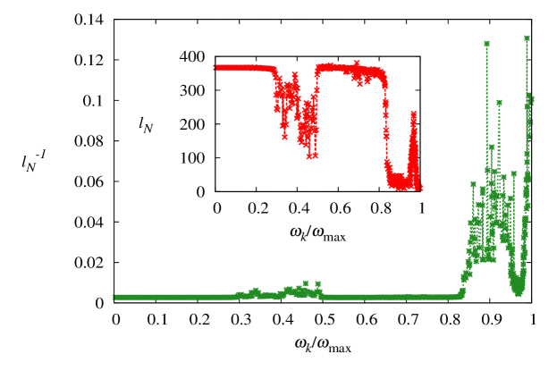
Figure 1: Inverse entropic localisation length $l_{N}^{-1}$ versus $\omega_{k}/\omega_{\rm max}$. The inset shows the entropic localisation length $l_{N}$ versus $\omega_{k}/\omega_{\rm max}$. The data were obtained for a chain with $N=500$ masses and disorder strength $\sigma^{2}/M^{2}=0.01$.

The entropic localisation length, first applied in [17] to quantum chaos, is a measure of the effective number of the eigenvector components significantly different from zero. Specifically, the inverse entropic localisation length for an eigenmode with displacement vector $e^{(i)}$ is defined as $l_{N}(\omega_{i})=\exp\left[S_{N}(\omega_{i})\right]$ where $S_{N}(\omega_{i})=-\sum_{k=1}^{N}\left[e_{k}^{(i)}\right]^{2}\log\left[e_{k}^{(i)}\right]^{2}$ is the Shannon entropy associated to the $i$-th mode. For localised eigenmodes, the entropic localisation length is proportional to the localisation length computed in the infinite-chain limit. Fig. 1 shows the inverse entropic localisation length for a random chain for which the binary correlator (20) has the form

$$\chi(l)=\frac{1}{2\left(\kappa_{2}-\kappa_{1}\right)l}\left[\sin\left(2\kappa_{2}l\right)-\sin\left(2\kappa_{1}l\right)\right]$$ (24)

exhibiting the power-law decay typical of long-range correlated disorder.

4 Anomalous transport properties of the chain with correlated disorder

We can now analyse how the delocalised modes affect the heat transport along the chain. The effect is best understood in terms of the modal heat flows (18) and (19). In figs. 2 and 3 we show the average modal flows in the stationary regime for fixed and free boundary conditions (the average was taken over 1000 disorder realisations).

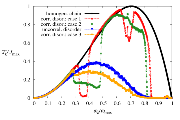
Figure 2: Average modal fluxes $\overline{J_{k}}/J_{\rm max}$ versus normalised frequency $\tilde{\omega}_{k}$ (fixed boundary conditions). $J_{\rm max}$ is the largest modal flux.

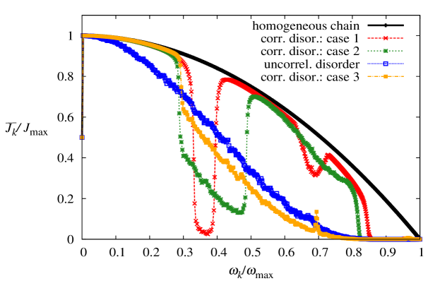
Figure 3: Average modal fluxes $\overline{J_{k}}/J_{\rm max}$ versus normalised frequency $\tilde{\omega}_{k}$ (free boundary conditions). $J_{\rm max}$ is the largest modal flux.

In both figures we show the modal fluxes for several kinds of harmonic chains: a homogeneous chain, a chain with uncorrelated disorder, and three chains with long-range correlated disorder. The latter cases of correlated disorder, which we refer to as case 1, 2, and 3, have localised modes in two windows $[\omega_{1}:\omega_{2}]$ and $[\omega_{3}:\omega_{4}]$, and extended modes in the complementary frequency intervals. In case 1, the limits of the localisation windows are $\tilde{\omega}_{1}=0.35,\,\tilde{\omega}_{2}=0.4,\,\tilde{\omega}_{3}\simeq 0.916,\,\tilde{\omega}_{4}\simeq 0.937$, where $\tilde{\omega}_{i}=\omega_{i}/\omega_{\rm max}$. In case 2 we enlarge the windows of localised modes, setting their limits at $\tilde{\omega}_{1}=0.3,\,\tilde{\omega}_{2}=0.5,\,\tilde{\omega}_{3}\simeq 0.866,\,\tilde{\omega}_{4}\simeq 0.954$. Finally, in case 3 we merge the localised-mode intervals by setting $\omega_{2}=\omega_{3}$; we thus generate a unique window $[\omega_{1},\omega_{4}]$ of localised modes with edges $\tilde{\omega}_{1}=0.3,\,\tilde{\omega}_{4}\simeq 0.954$.

In all cases the chain consists of $N=500$ masses and the disorder strength is $\sigma^{2}/M^{2}=0.01$. As can be seen from figs. 2 and 3, the heat transport is effectively suppressed in the windows of localised modes, being close to that of the homogeneous chain in the windows of extended modes. By an appropriate selection of the windows of localised and extended modes, one can either enhance (as in case 1 and 2) or suppress (as in case 3) the heat flow as compared with the case of uncorrelated disorder.

The delocalisation of normal modes induced by long-range correlations of the isotopic disorder has repercussions on the conductivity of the random chain. The most striking consequence is that, by increasing the number of delocalised modes in the medium-to-high frequency regions, one can obtain random chains which behave more and more as homogenous chains. In particular, the conductivity of such random chains scales as $\varkappa\propto N$, regardless of the chosen boundary conditions.

To understand this effect, let us focus on the case in which long-range correlated disorder produces extended modes in a frequency window $[\omega_{2},\omega_{3}]$. In the limit $N\gg 1$, the total heat flow can be approximated with the sum of the modal fluxes (18) over the frequency window $[\omega_{2},\omega_{3}]$. Assuming that the delocalised eigenmodes are not substantially altered with respect to the homogeneous case (a conjecture confirmed by numerical simulations for the weak-disorder case), one obtains that the heat flow in the stationary regime is

$$J_{\rm cd}\simeq\frac{\lambda k_{B}(T_{+}-T_{-})}{2M}\sum_{k=k_{2}}^{k_{3}}\left[e_{1}^{(k)}\right]^{2}\sim\frac{\lambda k_{B}(T_{+}-T_{-})}{2M}.$$ (25)

By dividing the flow (25) for the temperature gradient $(T_{+}-T_{-})/N$, one obtains that the effective conductivity of such a chain scales as $\varkappa_{\rm cd}\sim N$, as is the case for a homogeneous chain, and in contrast with the behaviour of a totally random chain. For the latter, heat transport is essentially due to the $O(N^{1/2})$ low-frequency modes and one has $\varkappa_{\rm ud}\sim N^{-1/2}$ for fixed boundary conditions and $\varkappa_{\rm ud}\sim N^{1/2}$ for free boundary conditions [1].

Our predictions are confirmed by the numerical data. To analyse the scaling law of the conductivity, we assumed an asymptotic behaviour of the form $\varkappa=AN^{\alpha}$ with $\alpha$ and $A$ constants. We numerically computed the conductivity $\varkappa$ for chains of length ranging from $N=200$ to $N=1000$ (with disorder strength $\sigma^{2}/M^{2}=0.01$). By fitting the data for $\log\varkappa$ versus $\log N$, we obtained values close to one for the exponent $\alpha$. Specifically, in the case of fixed boundary conditions we respectively obtained $\alpha_{\rm fix}^{(1)}=0.93\pm 0.01$ and $\alpha_{\rm fix}^{(2)}=0.84\pm 0.02$ for the cases 1 and 2 of correlated disorder. In the same cases, for free boundary conditions, the fitting values were $\alpha_{\rm free}^{(1)}=0.96\pm 0.01$ and $\alpha_{\rm free}^{(2)}=0.87\pm 0.01$. These results show that, when long-range correlations delocalise a finite fraction of medium-to-high frequency modes (as in case 1 and 2), the enhanced conductivity does scale as in the case of a homogeneous chain. Especially in case 1, with a larger number of delocalised modes, the critical exponent takes values very close to unity and is essentially independent from the boundary conditions.

We would like to stress that the enhancement or reduction of the conductivity manifests itself in the time domain, through the change of the speed with which the system relaxes to equilibrium or approaches the steady-state regime. By increasing the number of delocalised modes in the medium-to-high frequency region, one can significantly speed up the approach to the steady-state condition. This can be seen in fig. 4 which represents the evolution of the temperature of the central mass of a chain of $N=501$ atoms connected to two baths at the temperature $T=100$. All the masses of the chains were initially at rest in their equilibrium positions, and the evolution of the temperature was computed using eq. (16).

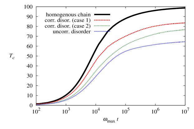
Figure 4: Time evolution of the temperature $T_{c}$ of the central atom of a random chain versus $\omega_{\rm max}t$ (log-scale).

The data shown in Fig. 4 were obtained for the coupling constant $\lambda=0.01$ and disorder strength $\sigma^{2}/M^{2}=0.01$. Fixed boundary conditions were chosen; the results, however, turn out to be qualitatively the same for free boundary conditions.

5 Conclusions

This work analyses the heat conduction in a random chain coupled to thermal baths. We focus on the problem of how specific long-range correlations of the disorder influence the thermal properties of the model. We show that long-range correlations of the disorder can delocalise a finite fraction of vibrational modes in the middle region of the frequency spectrum even for chains of relatively modest length ($N\gtrsim 300$). These delocalised modes modify both the approach to the stationary regime and the steady-state thermal properties of the chain. The larger the number of extended modes, the faster the chain tends to reach the steady-state condition and the closer the thermal properties are to those of a homogeneous chain. In particular, when the conductivity is enhanced it exhibits anomalous scaling $\varkappa\propto N^{\alpha}$ with $\alpha\sim 1$, independently of the boundary conditions. The long-range correlations of the disorder can also be used to strengthen the localisation of the chain eigenmodes: in this way one obtains a chain which is a better thermal insulator than a random chain with uncorrelated isotopic disorder.

I.F.H.-G. and L.T. gratefully acknowledge the support of the CONACyT grant No. 84604 and of the CIC-2009 grant (Universidad Michoacana). The work of F.M.I. was partly supported by CONACyT grant No. 80715.

References

- [1] Lepri S., Livi R., Politi A., Phys. Rep., 377, 1 (2003)
- [2] Dhar A., Advan. Phys., 57, 457 (2008)
- [3] Soukoulis C. M., Velgakis M. J., Economou E. N., Phys. Rev. B, 50, 5110 (1994); Bellani V., Diez E., Hey R., Toni L., Tarricone L., Parravicini G. B., Domínguez-Adame F., Gómez-Alcalá R., Phys. Rev. Lett., 82, 2159 (1999); Deych L. I., Erementchouk M. V., Lisyansky A. A., Phys. Rev. Lett., 90, 126601 (2003); Esmialpour A., Esmaeilzadeh M., Faizabadi E., Carpena P., Tabar M. R. R., Phys. Rev. B, 74, 024206 (2006); Sanchez-Palencia L., Clément D., Lugan P., Bouyer P., Shlyapnikov G. V., Aspect A., Phys. Rev. Lett., 98, 210401 (2007); Lugan P., Aspect A., Sanchez-Palencia L., Delande D., Grémaud B., Müller C. A. Miniatura C., Phys. Rev. A, 80, 023605 (2009)
- [4] de Moura F. A. B. F., Lyra M. L., Phys. Rev. Lett., 81, 3735 (1998); de Moura F. A. B. F., Lyra M. L., Phys. Rev. Lett., 84, 199 (2000)
- [5] Izrailev F. M., Krokhin A. A., Phys. Rev. Lett., 82, 4062 (1999)
- [6] Izrailev F. M., Krokhin A. A., Ulloa S. E. Phys. Rev. B, 63, 041102(R) (2001)
- [7] Izrailev F. M., Makarov N. M. J. Phys. A: Math. Gen., 38, 10613 (2005)
- [8] Tessieri L., Izrailev F. M., J. Phys. A: Math. Gen., 39, 11717 (2006)
- [9] Kuhl U., Izrailev F. M., Krokhin A. A., Stöckmann H.-J., Appl. Phys. Lett., 77, 633 (2000); Kuhl U., Izrailev F. M. Krokhin A. A., Phys. Rev. Lett., 100, 126402 (2008)
- [10] Krokhin A., Izrailev F., Kuhl U., Stöckmann H.-J., Ulloa S. E., Physica E, 13, 695 (2002)
- [11] de Moura F. A. B. F., Coutinho-Filho M.D., Raposo E. P., Lyra M. L., Phys. Rev. B, 68, 012202 (2003)
- [12] Shima H., Nishino S., Nakayama T., J. Phys.: Conference Series, 92, 012156 (2007)
- [13] Casher A., Lebowitz J. L., J. Math. Phys. (N.Y.), 12, 1701 (1971); O’Connor A. J., Lebowitz J. L., J. Math. Phys. (N.Y.), 15, 692 (1974)
- [14] Matsuda H., Ishii K., Suppl. Prog. Theor. Phys., 45, 56 (1970)
- [15] Arnold L., “Stochastic Differential Equation”, John Wiley and Sons, New York (1974)
- [16] Visscher W. M., Progr. Theor. Phys., 46, 729 (1971)
- [17] Izrailev F. M., Phys. Lett. A, 134, 13 (1988); Izrailev F. M., J. Phys. A: Math. Gen., 22, 865 (1989); Casati, G., Guarneri, I., Izrailev, F. M., Scharf R., Phys. Rev. Lett., 64, 5 (1990)