Cosmic microwave background constraints on cosmological models
with large-scale isotropy breaking

Abstract

Several anomalies appear to be present in the large-angle cosmic microwave background (CMB) anisotropy maps of WMAP, including the alignment of large-scale multipoles. Models in which isotropy is spontaneously broken (e.g., by a scalar field) have been proposed as explanations for these anomalies, as have models in which a preferred direction is imposed during inflation. We examine models inspired by these, in which isotropy is broken by a multiplicative factor with dipole and/or quadrupole terms. We evaluate the evidence provided by the multipole alignment using a Bayesian framework, finding that the evidence in favor of the model is generally weak. We also compute approximate changes in estimated cosmological parameters in the broken-isotropy models. Only the overall normalization of the power spectrum is modified significantly.

I Introduction

Our understanding of cosmology has advanced extremely rapidly in the past decade. These advances are due in large part to observations of cosmic microwave background (CMB) anisotropy, particularly the data from the Wilkinson Microwave Anisotropy Probe (WMAP) Hinshaw et al. (2003); Bennett et al. (2003); Hinshaw et al. (2007); Jarosik et al. (2010). As a result of these and other observations, a “standard model” of cosmology has emerged, consisting of a Universe dominated by dark energy and cold dark matter, with a nearly scale-invariant spectrum of Gaussian adiabatic perturbations Larson et al. (2010); Komatsu et al. (2010) of the sort that would naturally be produced in an inflationary epoch.

The overall consistency of the CMB data with this model is quite remarkable. In particular, the CMB observations are very nearly Gaussian, and the angular power spectrum matches theoretical models very well from scales of tens of degrees down to arcminutes. However, several anomalies have been noted on the largest angular scales, including a lack of large-scale power Bennett et al. (2003); Copi et al. (2007); de Oliveira-Costa et al. (2004), alignment of low-order multipoles Copi et al. (2004); Schwarz et al. (2004); de Oliveira-Costa et al. (2004); Hajian (2007), and hemispheric asymmetries Eriksen et al. (2004a); Freeman et al. (2006); Hansen et al. (2009). Some anomalies seem to be associated with the ecliptic plane, suggesting the possibility of a systematic error associated with the WMAP scan pattern, perhaps related to coupling of the scan pattern with the asymmetric beam Hanson et al. (2010). If the anomalies have cosmological significance, then naturally the correlation with the ecliptic plane must be a coincidence.

The significance of and explanations for these puzzles are hotly debated. In particular, it is difficult to know how to interpret a posteriori statistical significances: when a statistic is invented to quantify an anomaly that has already been noticed, the low $p$-values for that statistic cannot be taken at face value.

One can (and from a formal statistical point of view, arguably one must) dismiss this entire subject on the ground that all such anomalies are characterized only by invalid a posteriori statistics Bennett et al. (2010). Nonetheless, the number and nature of the anomalies (in particular, the fact that several seem to pick out the same directions on the sky) seem to suggest that there may be something to explain in the data. Given the potential importance of new discoveries about the Universe’s largest observable scales, and the difficulty in obtaining a new data set that would allow for a priori statistical analysis, we believe that the potential anomalies are worth further examination. In this paper, we will tentatively assume that there is a need for an explanation and consider what that explanation might be.

One of the most robust of the large-scale anomalies found in WMAP is a lack of large-scale power, as quantified either by the low quadrupole or the vanishing of the two-point correlation function at large angles Bennett et al. (2003); Copi et al. (2007); de Oliveira-Costa et al. (2004). If this anomaly is real, then it provides strong evidence against a broad class of nonstandard models. To be specific, all models in which a statistically independent contaminant (whether due to a foreground, systematic error, or exotic cosmology) is added to the data will necessarily fare worse than the standard model in explaining this anomaly Gordon et al. (2005); Bunn and Bourdon (2008). There is a simple reason for this: a statistically independent additive contaminant always increases the root-mean-square power in any given mode, reducing the probability of finding low power.

It is natural, therefore, to seek an explanation of the anomalies among models that do not involve a mere additive contaminant. One simple phenomenological model is a multiplicative contaminant, in which the original statistically isotropic CMB signal $T^{(0)}(\theta,\phi)$ is modulated by a multiplicative factor, leading to an observed signal

$$T(\theta,\phi)=f(\theta,\phi)T^{(0)}(\theta,\phi).$$ (1)

This model arises naturally in the framework of spontaneous isotropy breaking by a scalar field Gordon et al. (2005). Moreover, models based on the existence of a vector field specifying a preferred direction during inflation Ackerman et al. (2007); Böhmer and Mota (2008) produce similar modulation, but with $f$ having specifically a quadrupolar form. To be precise, the modulation in these models takes place in the primordial power spectrum $P(\vec{k})$, which acquires a quadrupolar dependence on the direction of $\vec{k}$. The full effect on the CMB anisotropy is more complicated than the above model, but the dominant effect on large scales is, at least approximately, a quadrupolar moduloation of the above form.

Since our goal is to explain the observed large-scale anomalies while maintaining the success of the standard model on smaller scales, it is natural to consider models in which $f$ has power only on large scales. We will consider three classes of model: one in which $f$ has only monopole and dipole terms, one in which it has monopole and quadrupole, and one in which it has all three. We will refer to these as the dipole-only, quadrupole-only, and dipole-quadrupole models. The quadrupole-only model is inspired by the theory of a preferred direction during inflation, while the others are inspired by the general isotropy-breaking framework.

This paper addresses the following central question. Do the broken-isotropy models provide an explanation for one of the main observed anomalies, namely the surprising alignment between the quadrupole and octupole (multipoles $l=2,3$)? To examine this question, we choose statistics to quantify the anomaly and use these statistics to assess goodness of fit of the data to the different models. Several different statistics are chosen in order to assess the robustness of the results.

Because the statistics are most naturally computed in spherical harmonic space, we use the all-sky internal linear combination (ILC) maps from the five-year WMAP data release Hinshaw et al. (2008). There is bound to be residual foreground contamination in the ILC maps Eriksen et al. (2004b); Eriksen et al. (2005). Section VI contains a brief discussion of the effects of this contamination.

Naturally, because the anisotropic models have more free parameters than the standard model (and indeed include the standard model as a special case), there will generically be parameter choices that make the anisotropic model fit the data better. We adopt the Bayesian evidence criterion to assess whether this improved fit is sufficient to justify the additional complexity of the anisotropic model. Bayesian evidence has been used in addressing this sort of question in the past Land and Magueijo (2007); Eriksen et al. (2007); Hoftuft et al. (2009). Although some controversy has arisen over its use in cosmology (e.g., Marshall et al. (2006); Liddle et al. (2006); Liddle (2007); Efstathiou (2008)), in this context it is both a simple and a natural criterion to adopt.

In some cases, the Bayesian evidence ratios are greater than one, meaning that one’s assessment of the probability that the broken-isotropy models are true should rise as a result of the CMB anomalies. However, in all cases, the improvement is modest, providing at most weak support for the adoption of the anisotropic models.

We also consider the changes in parameter estimates that would arise if the anisotropic models are correct. To be specific, because we assume that the modulation is a perturbation to the standard model, we assume that the unmodulated temperature map $T^{(0)}$ is derived from the cosmological parameters in the usual way – i.e., its power spectrum is given by CMBFAST Seljak and Zaldarriaga (1996). If there is a nonconstant modulation function $f$, then parameter estimates from based on the observed data will naturally differ from the true values. We estimate the resulting parameter shifts, finding them to be minor.

The remainder of this paper is structured as follows. Section II specifies precisely the anisotropic models under consideration and describes how we simulate these models. In Section III, we review the method for computing Bayesian evidence ratios. Section IV contains our main results, indicating the degree to which the multipole alignment, quantified in several different ways, favor the broken-isotropy models. In Section V we quantify the degree to which best-fit cosmological parameters are modified by changing from the standard model to the broken-isotropy models. Section VI discusses some aspects of the issue of foreground contamination. Finally, we provide a brief discussion of our results in Section VII.

II Simulating anisotropic models

The statistical properties of a CMB map are most easily expressed in terms of the spherical harmonic expansion,

$$T(\theta,\phi)=\sum_{l=0}^{\infty}\sum_{m=-l}^{l}a_{lm}Y_{lm}(\theta,\phi).$$ (2)

The monopole ($l=0$) term in the sum is simply the average temperature over the sky, and the dipole ($l=1$) terms cannot be separated from the kinematic dipole due to our motion with respect to the CMB “rest” frame. These terms are typically removed from the data, so that in practice the sum starts at $l=2$. For compactness, we will generally abbreviate such double sums as $\sum_{l,m}$, not writing the limits explicitly unless confusion may arise.

In the standard model, the CMB map $T^{(0)}(\theta,\phi)$ is a realization of a statistically isotropic Gaussian random process. This means that the spherical harmonic coefficients $a^{(0)}_{lm}$ of this map are independent Gaussian random variables with mean zero and variances that depend only on $l$:

$$\langle|a^{(0)}_{lm}|^{2}\rangle=C_{l}^{(0)},$$ (3)

where $\langle\cdot\rangle$ denotes an ensemble average and $C_{l}^{(0)}$ is the power spectrum.

In broken-isotropy models, on the other hand, we assume that the observed field is related to the above statistically isotropic expression according to equation (1). We expand the modulation function in spherical harmonics,

$$f(\theta,\phi)=1+\sum_{l,m}f_{lm}Y_{lm}(\theta,\phi).$$ (4)

We assume that the modulation function is normalized to have mean one, so that the above sum starts at $l=1$. (Equivalently, we could omit the $1+$ in the above expression and start the sum at $l=0$ with $f_{00}=\sqrt{4\pi}$.) We will assume that the coefficients $f_{lm}$ are independent Gaussian random variables with a power spectrum

$$C_{l}^{(f)}\equiv\langle|f_{lm}|^{2}\rangle.$$ (5)

As noted in the Introduction, we consider models in which $f$ has only dipole and/or quadrupole terms. We parameterize these terms with parameters $\sigma_{1},\sigma_{2}$, giving the rms values of $f_{lm}$ relative to a scale-invariant spectrum $C_{l}^{(f)}\propto[l(l+1)]^{-1}$:

$$\sigma_{1}^{2}=2C_{1}^{(f)},\qquad\qquad\sigma_{2}^{2}=6C_{1}^{(f)}.$$ (6)

Because the spherical harmonics have root-mean-square (rms) value $(4\pi)^{-1/2}$, these modulations have rms amplitudes $(8\pi)^{-1/2}\sigma_{1}=0.20\sigma_{1}$ and $(24\pi)^{-1/2}\sigma_{2}=0.12\sigma_{2}$ respectively.

The spherical harmonic coefficients of the observed sky are found as usual by spherical harmonic orthonormality:

$$a_{lm} = \int d\Omega\,T(\theta,\phi)Y_{lm}^{*}(\theta,\phi)$$ (7)

$$= \int d\Omega\,f(\theta,\phi)T^{(0)}(\theta,\phi)Y_{lm}^{*}(\theta,\phi).$$ (8)

Expanding the functions $T^{(0)}$ and $f$ in spherical harmonics, we find that

$$a_{lm}=\sum_{l_{1},m_{1}}\sum_{l_{2},m_{2}}a_{l_{1}m_{1}}^{(0)}f_{l_{2}m_{2}}I_{l_{1}m_{1}l_{2}m_{2}lm},$$ (9)

where $I_{l_{1}m_{1}l_{2}m_{2}lm}$ represents an integral over three spherical harmonics, which ca be expressed in terms of Wigner 3-$j$ symbols Zare (1988):

$$I_{l_{1}m_{1}l_{2}m_{2}lm} \equiv \int Y_{l_{1}m_{1}}Y_{l_{2}m_{2}}Y_{lm}^{*}\,d\Omega$$ (11)

$$= \left[{\left(2l+1\right)\left(2l_{1}+1\right)\left(2l_{2}+1\right)\over 4\pi}\right]^{1\over 2}\times$$

$$\quad\begin{pmatrix}l&l_{1}&l_{2}\\ 0&0&0\end{pmatrix}\begin{pmatrix}l&l_{1}&l_{2}\\ -m&m_{1}&m_{2}\end{pmatrix}$$

The quadruple sum in equation (9) has very few nonzero terms and hence can be quickly evaluated. Because our model includes only low-$l$ power in $f$, the sum over $l_{2}$ ranges from 0 to at most 2. Moreover, the Wigner 3-$j$ symbols vanish unless certain conditions are satisfied. First, $(l,l_{1},l_{2})$ must satisfy a triangle inequality, so that the sum over $l_{1}$ ranges from $l-2$ (or zero, whichever is greater) to $l+2$. Second, the first of the two 3-$j$ symbols vanishes unless $l+l_{1}+l_{2}$ is even. Finally, the constraint $m=m_{1}+m_{2}$ must be satisfied.

III Bayesian evidence

Our goal in this paper will be to compare the standard model (the null hypothesis) with the class of broken-isotropy models. Naturally, because the latter class is broader, and indeed includes the null hypothesis as a limiting case, there will generically be members of the class that fit the data better than the standard model. The Bayesian evidence provides a framework for assessing whether the better fit found in the more complicated model is worth the Occam’s-razor “cost.” We now briefly review this approach to model comparison.

Suppose that we have a model $M$ that depends on a set of parameters $\boldsymbol{\theta}$. Given a data set $D$, we define the evidence of the model to be the probability density of $D$, given the model $M$:

$$E(M)=\int d\boldsymbol{\theta}\,P(D|M,\boldsymbol{\theta})\pi(\boldsymbol{\theta}|M).$$ (12)

In this expression, $P$ is the likelihood function – that is, the probability density for the data given the choice of model and parameters – and $\pi$ is the prior probability density of the model parameters. It may be helpful to keep track of dimensions in these expressions. The prior $\pi$ has dimensions of probability per unit volume in parameter space, while $P$ and $E$ have dimensions of probability per unit volume in data space.

Bayes’s theorem says that the posterior probability of the model is proportional to the product of the model’s prior probability and the evidence. Suppose now that we have two models $M_{1},M_{2}$ in mind, and imagine that, before looking at the data set $D$, we regarded these models as equally probable. Then the evidence ratio

$$\Lambda\equiv{E(M_{1})\over E(M_{2})}$$ (13)

is equal to the ratio of posterior probabilities.

In the case we consider in this paper, the two models are the standard model and the broken-isotropy model. The reader (like the writers) probably does not assign equal prior probabilities to these two models: in the absence of the WMAP anomalies, most of us probably thought that the broken-isotropy model was less likely. Even in this case, the evidence ratio still tells us by what factor the broken-isotropy model goes up in our estimation (relative to the isotropic model) as a result of the data.

The Bayesian evidence automatically accounts for the degree of complexity of the model, in the sense that models with a large parameter space will be automatically downweighted compared to those with a small parameter space. To see this heuristically, suppose that the prior probability $\pi$ is approximately flat over some volume $V_{p}$ in parameter space that is much larger than the range over which the likelihood function is large. Then since the probability distribution is normalized,

$$\int d\boldsymbol{\theta}\,\pi(\boldsymbol{\theta}|M)=1,$$ (14)

we can estimate $\pi\sim V_{p}^{-1}$ over the range where the integrand is significant. Thus we can crudely estimate

$$E(M)\sim V_{p}^{-1}\int d\boldsymbol{\theta}\,P(D|M,\boldsymbol{\theta})\sim{P_{\rm max}V_{L}\over V_{p}},$$ (15)

where $P_{\rm max}$ is the peak of the likelihood function and $V_{L}$ is an estimate of the volume in parameter space over which the likelihood differs significantly from zero. If we consider two models with similarly good fits to the data (i.e., similar values of $P_{\rm max}$), the one with a higher value of the ratio $V_{p}/V_{L}$ will have the higher value of the evidence. In other words, the Bayesian evidence disfavors models with a large volume of “wasted” parameter space. When comparing models with parameter spaces of different dimensions, the one with a higher-dimensional parameter space will typically be disfavored, unless it provides a much better fit to the data (i.e., has a large $P_{\rm max}$) or it provides a reasonably good fit to the data over most of the parameter space.

Below, we will use Bayesian evidence ratios to assess whether the multipole alignment anomaly significantly favors the adoption of the more complicated broken-isotropy models, using the following procedure. We define a statistic $s$ that describes the anomaly. Since the null (statistically isotropic) hypothesis $M_{0}$ has no free parameters, the evidence for it is simply the probability density of the statistic under that hypothesis:

$$E_{0}=P(s|M_{0}).$$ (16)

For some choices of statistic, this probability density can be computed analytically, but in general it must be estimated from simulations.

(a)	(b)

Figure 1: (a) Values of the probability density function (pdf) for the multipole alignment statistic $\lambda$, evaluated in an interval of width $\delta\lambda=0.02$ about $\lambda=0.985$, from $10^{4}$ simulations for each choice of parameter values. The different curves correspond to $\sigma_{2}=(0,e^{-1},1,e,e^{2},e^{3})=(0,0.37,1,2.7,.7.4,20)$ (from highest to lowest pdf at the right of the plot). (b)The Bayesian evidence for the anisotropic models. The solid curve is for the dipole-only model, the dashed curve is for the dipole-quadrupole model, and the dotted curve is for the quadrupole-only model.

We now consider the evidence $E_{1}\equiv E(M_{1})$ for the broken-isotropy model. Let us first examine the models in which $f$ has only power in one multipole (i.e., the dipole-only and quadrupole-only models). The parameter space $\boldsymbol{\theta}$ for this model consists of the single parameter $\sigma_{j}$, where $j=1$ for the dipole-only model and 2 for the quadrupole-only model. To compute the evidence for this model, we must choose a prior $\pi(\sigma_{j})$. We adopt a uniform prior on some range $\sigma_{j}\in[0,\sigma_{\rm max}]$:

$$\pi(\sigma_{j})=\begin{cases}\sigma_{\rm max}^{-1}&0<\sigma_{j}<\sigma_{\rm max},\\ 0&\mbox{otherwise.}\end{cases}$$ (17)

For the dipole-quadrupole model, we follow a similar procedure, adopting a prior on $\boldsymbol{\theta}=(\sigma_{1},\sigma_{2})$ of

$$\pi(\sigma_{1},\sigma_{2})=\begin{cases}\sigma_{\rm max}^{-2}&0<\sigma_{1},\sigma_{2}<\sigma_{\rm max},\\ 0&\mbox{otherwise.}\end{cases}$$ (18)

Since it is not obvious what cutoff $\sigma_{\rm max}$ to choose, we plot the evidence ratio $E_{1}/E_{0}$ as a function of this parameter. We regard the maximum value of the evidence ratio as an upper bound on the true evidence ratio. From the heuristic argument above we expect the evidence ratio to decline for very large values of $\sigma_{\rm max}$, since these models presumably have “wasted” parameter space.

IV Results

Various statistics have been used in the past to characterize the observed alignment of the $l=2$ and $l=3$ multipoles in the WMAP data. We focus on two categories of statistic: one based on finding the directions that maximize the angular momentum de Oliveira-Costa et al. (2004) for each multipole (Section IV.1), and one based on multipole vectors Schwarz et al. (2004); Copi et al. (2004) (Section IV.2).

IV.1 Angular momentum

For any given multipole $l$, consider the map obtained by keeping just the corresonding coefficients in the spherical harmonic expansion,

$$T_{l}(\theta,\phi)=\sum_{m=-l}^{l}a_{lm}Y_{lm}(\theta,\phi).$$ (19)

The maps $T_{2}$ and $T_{3}$ are each observed to have fluctuations that lie predominantly in a single plane, and moreover the planes associated with these two multipoles seem to be aligned Schwarz et al. (2004); Copi et al. (2004); de Oliveira-Costa et al. (2004); Hajian (2007). The idea of the maximum-angular-momentum statistic is to quantify that alignment by defining for each $l$ an axis perpendicular to the plane picked put by the map $T_{l}$.

Consider a particular map $T_{l}$. For any given direction, specified by a unit vector $\hat{{n}}$, we imagine rotating the map to bring $\hat{{n}}$ to the $z$ axis. Let $a_{lm}^{R}$ represent the spherical harmonics in the rotated coordinate system, which can be efficiently computed by applying an appropriate Wigner $D$ matrix to the unrotated $a_{lm}$’s Zare (1988). We compute the the “angular momentum” of the rotated map about the $z$ axis:

$$L_{z}^{2}(\hat{{n}})=\sum_{m=-l}^{l}m^{2}|a_{lm}^{R}|^{2}.$$ (20)

The direction $\hat{{n}}$ that maximizes $L_{z}^{2}$ is taken to be the axis $\hat{{n}}_{l}$ for the given multipole. Note that because $L^{2}_{z}(\hat{{n}})=L^{2}_{z}(-\hat{{n}})$, the vector $\hat{{n}}_{l}$ is only defined up to an overall sign.

We use the statistic $\lambda=|\hat{{n}}_{2}\cdot\hat{{n}}_{3}|$ to assess the degree to which the fluctuations in the quadrupole and octupole are aligned. In any statistically isotropic model, we expect the directions $\hat{n}_{l}$ to be indepent and uniformly distributed over the unit sphere, which implies that $\lambda$ is uniformly distributed on the interval $[0,1]$. The value in the actual WMAP data is surprisingly large at $\lambda_{\mbox{\scriptsize WMAP}}=0.985$.

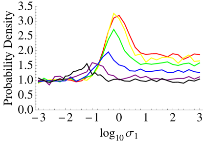
For any given choice of parameters $(\sigma_{1},\sigma_{2})$, we can simulate a large number of maps and determine the probability density function (pdf) of the statistic $\lambda$. Specifically, we can estimate the average pdf in an interval of with $\delta\lambda$ around the value $\lambda_{\mbox{\scriptsize WMAP}}$ simply by finding the fraction of all simulations yielding values in the range $[\lambda_{\mbox{\scriptsize WMAP}}-{1\over 2}\delta\lambda,\lambda_{\mbox{\scriptsize WMAP}}+{1\over 2}\delta\lambda]$. Figure 1a shows the resulting pdfs, based on $10^{4}$ simulations for each point in parameter space, with $\delta\lambda=0.02$. The Poisson noise in this estimation process is visible as $\sim 7\%$ scatter in the points in this plot. Histograms of the simulation results confirm that the pdfs are smooth over scales much larger than $\delta\lambda$, so interpreting the average pdf as the pdf at the given point is reasonable.

(a)	(b)

Figure 2: (a) Probability density for the Schwarz et al. Schwarz et al. (2004) multipole vector statistic $S$, evaluated at the value found in the WMAP data. From top to to bottom at $\log_{10}\sigma_{1}=0$, the curves correspond to $\sigma_{2}=(0,0.25,0.50,1.,2.0,4.0,16)$. (b) Bayesian evidence for anisotropic models. Results are plotted for the dipole-quadrupole (solid), dipole-only (dashed), and quadrupole-only (dotted) models.

Since the pdf under the null hypothesis is equal to 1, this quantity can be interpreted as a Bayesian evidence ratio comparing the model with the given values of $(\sigma_{1},\sigma_{2})$ to the null hypothesis.

As Figure 1a shows, for some choices of parameter, the evidence ratio exceeds $3$. However, this overstates the evidence in favor of the broken-isotropy model. As described in Section III, the correct procedure is to treat $\sigma_{1},\sigma_{2}$ as unknown parameters with a given prior distribution, and integrate over that prior to get the evidence. The integration is performed numerically, after interpolating between the likelihood estimates found for the various values of $(\sigma_{1},\sigma_{2})$.

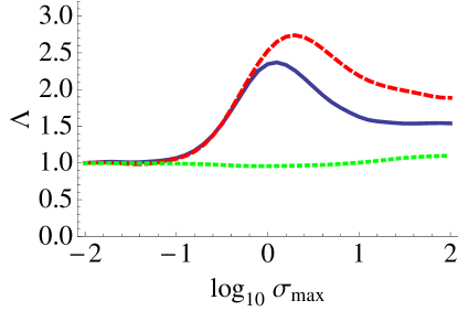
Figure 1b shows the result of this calculation. The quantity on the horizontal axis is the prior cutoff $\sigma_{\rm max}$ of equation (17) or (18). Because each Bayesian evidence ratio is an integral over the likelihood function, the effect of Poisson noise due to the finite number of simulations is greatly reduced.

In the dipole-quadrupole case (where both $\sigma_{1},\sigma_{2}$ are free parameters), the Bayesian evidence ratio has a maximum value of $\sim 2.4$ at $\sigma_{\rm max}\sim 1$. (Recall that, as noted in Section II, $\sigma=1$ corresponds to only 10-20% modulation.) The dipole-only model (in which only $\sigma_{1}$ varies) fares a bit better, with evidence ratio peaking at $\sim 2.7$. Even if we take this maximum value as the true evidence ratio, it is still only modest support for the broken-isotropy model. The quadrupole-only model shows no significant improvement at all over the standard model (as we could have predicted from Figure 1a, in which all curves approach the standard-model value of 1 for low $\sigma_{1}$).

IV.2 Multipole vectors

To test the robustness of this result, we can use a different approach to quantify the multipole alignment. For each multipole $l$, the map $T_{l}$ can be used to define $l$ unit vectors, generally called “multipole vectors” Copi et al. (2004). The multipole vectors for each $l$ can be used to characterize the orientation of that multipole, and thus to characterize the quadrupole-octupole alignment.

There are multiple different ways of using the multipole vectors to define an alignment statistic. The original work on the subject Copi et al. (2004) used an elaborate procedure involving the assessment of several different combinations of dot and cross products of the multipole vectors. Subsequent work by members of the same group Schwarz et al. (2004) focused on a smaller subset of these possibilities. We have chosen to implement the “robust and more conservative” statistic used in the latter work. We now describe this statistic.

Let $\hat{{v}}^{(l,j)}$ ($1\leq j\leq l$) represent the $j$th multipole vector for multipole $l$. For any given $l$, we consider all $l(l-1)/2$ distinct cross products of multipole vectors $\vec{w}^{(l,i,j)}\equiv\hat{v}^{(l,i)}\times\hat{v}^{(l,j)}$ ($1\leq i<j\leq l$). Alignment of the quadrupole and octupole planes can be characterized by the absolute values of the dot product of the one quadrupole cross product, $\hat{w}^{(2,1,2)}$, with each of the three octupole cross products $\hat{w}^{(3,i,j)}$. (The absolute value is necessary because the multipole vectors, and hence the cross products, are specified only up to an overall sign.) Following ref. Schwarz et al. (2004), we therefore define a statistic

$$S=|\vec{w}^{(2,1,2)}\cdot\vec{w}^{(3,1,2)}|+|\vec{w}^{(2,1,2)}\cdot\vec{w}^{(3,1,3)}|+|\vec{w}^{(2,1,2)}\cdot\vec{w}^{(3,2,3)}|$$ (21)

The value of this statistic for the WMAP data is $S_{\mbox{\scriptsize WMAP}}=2.233$. Based on Monte Carlo simulations, we find this to be inconsistent with the standard isotropic model at $99.3\%$ confidence. These values differ only slightly from those found in ref. Schwarz et al. (2004) ($S_{\mbox{\scriptsize WMAP}}=2.396$, ruled out at $99.87\%$ confidence), which used an earlier data release and a different foreground removal process Tegmark et al. (2003).

(a)	(b)

Figure 3: Bayesian evidence ratios calculated using multipole vectors. In (a), the joint probability density for $(A,p)$, the alignment and planarity statistics was used. In (b), only the statistic $A$ was used. Results are plotted for the dipole-quadrupole (solid), dipole-only (dashed), and quadrupole-only (dotted) models.

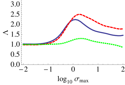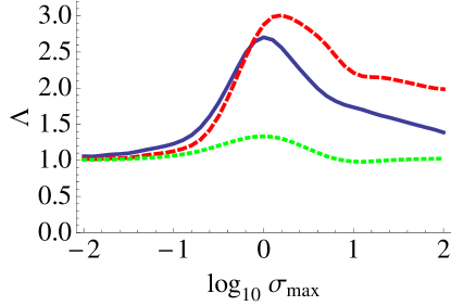
Figure 2 shows the result of Bayesian evidence calculations based on this statistic. At each point $(\sigma_{1},\sigma_{2})$ in parameter space, the pdf (i.e., the likelihood function) was evaluated from $10^{4}$ simulations, by counting the number of times the statistic was found in an interval of width $\delta S=0.15$ about the value found in the WMAP data. The results are qualitatively consistent with those based on the angular momentum statistic, although with slightly higher evidence ratios (i.e., slightly more favorable to the broken-isotropy models).

There is of course some arbitrariness in the choice of the statistic $S$. In addition to $S$, we devised an alternative set of statistics based on the multipole vectors. The results based on these statistics can be viewed as a test of the robustness of the results above.

In defining our statistics we were guided by a desire to characterize the observed dipole-quadrupole alignment and the fact that the octupole has been characterized as unusually planar. Since we were guided by these already-observed facts, of course, our choices are subject to the same a-posteriori-statistics criticism as most other work in this area. We did, however, attempt to avoid exacerbating this problem with further a posteriori choices: we devised our statistics blindly and used only one statistic to characterize each of these two phenomena.

The two multipole vectors at $l=2$ define a plane, and we let $\hat{n}_{2}$ be the unit vector perpendicular to that plane. To assess the multipole alignment, we need to define a similar unit vector based on the three $l=3$ vectors. We define $\hat{n}_{3}$ to be the unit vector that is as nearly as possible perpendicular to these vectors by minimizing the quantity

$$p=\sum_{1\leq i<j\leq 3}(\hat{n}_{3}\cdot\hat{v}^{(3,i,j)})^{2}.$$ (22)

As in the angular momentum case, we define an alignment statistic to be the absolute value of the dot product of these vectors:

$$A=|\hat{n}_{2}\cdot\hat{n}_{3}|.$$ (23)

In addition, the statistic $p$ can be thought of as characterizing the octupole planarity, with low values of $p$ corresponding to more planar octupole patterns.

The value of $A$ for the real data is 0.97, which is somewhat anomalously high since a uniform distribution on [0,1] is expected in the standard model. The statistic $p$, on the other hand, does not show anomalous planarity: its value in the real data is 0.31, lying near the middle of the distribution in simulations based on the standard model.

Since $p$ is quite consistent with the standard model, we would not expect its inclusion in our analysis to improve the evidence for any nonstandard models. For completeness, we performed the Bayesian evidence calculations using the joint probability density on $A$ and $p$ as our input likelihood function, and also using the probablility densities on $A$ and $p$ separately.

The probability densities for each parameter were calculated as with the previous statistics, by counting the number of simulations yielding values in a small interval about the value in the true data. In this case, we used $10^{5}$ simulations at each data point, with $\delta A=\delta p=0.005$. The joint probability density was estimated as the product of the individual pdfs. In principle, the two statistics could be correlated, in which case this would not be correct. In practice, however, correlations were found to be negligible for the models under consideration; in spot-checks this approximation was found to be quite good.

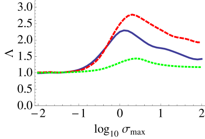
Figure 3 shows the result of Bayesian evidence computations based on this statistic. As expected, the results vary only slightly depending on whether the planarity statistic is included. In either case, the strongest evidence ratio comes at $\sigma_{\rm max}\approx 1$ in the dipole-only model, but as before the evidence ratios are modest, peaking at $\sim 2.7$ including both statistics and $\sim 2.5$ using only the alignment statistic. Results showing the planarity-only statistic are not shown but yield no significant enhancement in the evidence ratio.

The strong similarity in all of the evidence ratio plots suggests that our results are insensitive to the precise way that the multipole alignment is characterized.

V Corrections to cosmological parameters in anisotropic models

In the anisotropic models under consideration, the power spectrum $C_{l}$ is modified by the modulation function $f$. We assume that the original, unmodulated power spectrum $C_{l}^{(0)}$, as opposed to the measured power spectrum $C_{l}$, is produced by the usual standard-model mechanism. In the anisotropic models, therefore, the cosmological parameters estimated from the power spectrum will differ from those in the standard model. In this section we estimate the changes in parameters as functions of $\sigma_{1}$ and $\sigma_{2}$. To be specific, we will assume that $C_{l}$ has been estimated from the data and used to derive power spectrum estimates under the standard assumptions of isotropy and Gaussianity. We will compute the corrections that must be applied to these parameter estimates for nonzero $\sigma_{1},\sigma_{2}$. We find that for reasonable values of $\sigma_{1},\sigma_{2}$, all parameters except the overall normalization undergo very small changes.

The changes in parameter values we compute depend on the assumption that the modulation is the same across all angular scales. If the modulation exists only on large scales, with smaller scales described by the unmodulated standard model, then the changes in parameter estimates will be even smaller than those found here.

To estimate the changes in parameter values, we assume that the unmodulated CMB power spectrum is given by the standard model and can be calculated from, e.g., CMBFAST Seljak and Zaldarriaga (1996). We begin by deriving the relationship between the modulated (i.e., observed) power spectrum $C_{l}$, the unmodulated power spectrum $C_{l}^{(0)}$, and the power spectrum $C_{l}^{(f)}$ of the modulating function. We begin from equation (9):

$$a_{lm}=\sum_{l_{1},m_{1}}\sum_{l_{2},m_{2}}a_{l_{1}m_{1}}^{(0)}f_{l_{2}m_{2}}I_{ll_{1}l_{2}mm_{1}m_{2}},$$ (24)

where $I_{ll_{1}l_{2}mm_{1}m_{2}}$ is defined in equation (11).

Figure 4: Power spectrum changes. The solid curves are the $\delta C_{l}$’s resulting from nonzero $\sigma_{1}$ or $\sigma_{2}$ as described in equation (32). The dot-dashed curves are the results of the linear approximation (33), with best-fit $\delta g_{i}$. The dashed curves are are the $\delta C_{l}$’s resulting from recomputing the power spectrum with the modified parameter values. Power spectra are computed in dimensionless $(\Delta T/T)^{2}$ form. In these units, the CMB power is of order $10^{10}l(l+1)C_{l}/2\pi\sim 1.5$ - 8 over the multipole range of interest; thus in the top panels, the deviations in the power spectrum are all quite small. The different approximations agree reasonably well, showing that the approximations in this section are adequate.

In an isotropic model, the power spectrum is given by $C_{l}=\langle|a_{lm}|^{2}\rangle$, which is independent of $m$. In an anisotropic model, this quantity is not necessarily independent of $m$, so we define the power spectrum to be the average over $m$:

$$C_{l}={1\over 2l+1}\sum_{m}\langle|a_{lm}|^{2}\rangle.$$ (25)

We substitute equation (24) into this expression. We then make use of the fact that both the $a_{lm}^{(0)}$ and $f_{lm}$ coefficients are drawn from isotropic Gaussian random processes, which implies that different coefficients are uncorrelated:

$$\langle a_{lm}^{(0)}a_{l^{\prime}m^{\prime}}^{(0)*}\rangle = C_{l}^{(0)}\delta_{ll^{\prime}}\delta_{mm^{\prime}},$$ (26)

$$\langle f_{lm}f_{l^{\prime}m^{\prime}}^{*}\rangle = C_{l}^{(f)}\delta_{ll^{\prime}}\delta_{mm^{\prime}},$$ (27)

$$\langle a_{lm}^{(0)}f_{l^{\prime}m^{\prime}}^{*}\rangle = 0.$$ (28)

The result is

$$C_{l} = \sum_{l_{1},l_{2}}C_{l_{1}}^{(0)}C_{l_{2}}^{(f)}\left({1\over 2l+1}\sum_{m_{1},m_{2},m}I_{l_{1}l_{2}lm_{1}m_{2}m}^{2}\right)$$ (29)

$$\equiv \sum_{l_{1},l_{2}}C_{l_{1}}^{(0)}C_{l_{2}}^{(f)}\overline{I^{{}^{2}}}_{{}_{\!\!\!\!l_{1}l_{2}l}}.$$ (30)

The sum inside the parentheses is over all $m$, $m_{1}$, and $m_{2}$ values that make the Wigner 3-$j$ symbols physical. We assume that $C_{l_{2}}^{(f)}=0$ for $l_{2}>2$, so that the double sum above becomes three single sums:

$$C_{l} = \sum_{l_{1}}C_{l_{1}}^{(0)}C_{0}^{(f)}\overline{I^{{}^{2}}}_{{}_{\!\!\!\!l_{1}0l}}+\sum_{l_{1}}C_{l_{1}}^{(0)}C_{1}^{(f)}\overline{I^{{}^{2}}}_{{}_{\!\!\!\!l_{1}1l}}$$ (31)

$$\qquad\qquad+\sum_{l_{1}}C_{l_{1}}^{(0)}C_{2}^{(f)}\overline{I^{{}^{2}}}_{{}_{\!\!\!\!l_{1}2l}}$$

Because of the triangle inequality on the 3-$j$ symbols, the first sum contains only one nonzero term ($l_{1}=l$), and not surprisingly this term reduces to $C_{l}^{(0)}$. The second and third sums similarly have only a few nonzero terms.

Substituting $C_{1}^{(f)}={\sigma_{1}^{2}/2}$ and $C_{2}^{(f)}={\sigma_{2}^{2}/6}$, we find that the difference between modulated and unmodulated power spectra is

$$\delta C_{l}=C_{l}-C_{l}^{(0)}={\sigma_{1}^{2}\over 2}\sum_{l_{1}}C_{l_{1}}^{(0)}\overline{I^{{}^{2}}}_{{}_{\!\!\!\!l_{1}1l}}+{\sigma_{2}^{2}\over 6}\sum_{l_{1}=2}^{\infty}C_{l_{1}}^{(0)}\overline{I^{{}^{2}}}_{{}_{\!\!\!\!l_{1}2l}}$$ (32)

We see that $\delta C_{l}$ is a linear function of $\sigma_{1}^{2}$ and $\sigma_{2}^{2}$. For any given model, we can calculate the $\delta C_{l}$ contributions from $\sigma_{1}^{2}$ and $\sigma_{2}^{2}$ independently.

Assuming that the perturbation from the applied field is small, we expect the change in the power spectrum, and hence the change in the inferred parameter values, to be small. In the standard $\Lambda$CDM paradigm, the observed power spectrum depends on six parameters: $\Omega_{b}$ (baryon density), $\Omega_{\rm cdm}$ (dark matter density), $\Omega_{\Lambda}$ (vacuum energy density), $n$ (spectral index), $H_{0}$ (Hubble constant, $h={H_{0}/(100\,{\rm km\,s^{-1}\,Mpc})}$), and $A$ (normalization constant for all $C_{l}$, relative to the current best fit values from WMAP). Calling these parameters $g_{1},\ldots,g_{6}$, we have to a good approximation

$$\delta C_{l}\approx\sum_{i=1}^{6}\delta g_{i}{\partial C_{l}\over\partial g_{i}}$$ (33)

Setting equations (32) and (33) equal, and splitting the parameter variations into terms that depend on $\sigma_{1}$ and $\sigma_{2}$, we can write

$$\sum_{i=1}^{6}\delta g_{i,{\sigma_{1}^{2}}}{\partial C_{l}\over\partial g_{i}} \approx {\sigma_{1}^{2}\over 2}\sum_{l_{1}=2}^{\infty}C_{l_{1}}^{(0)}\overline{I^{{}^{2}}}_{{}_{\!\!\!\!l_{1}1l}}$$ (34)

$$\sum_{i=1}^{6}\delta g_{i,{\sigma_{2}^{2}}}{\partial C_{l}\over\partial g_{i}} \approx {\sigma_{2}^{2}\over 6}\sum_{l_{1}=2}^{\infty}C_{l_{1}}^{(0)}\overline{I^{{}^{2}}}_{{}_{\!\!\!\!l_{1}2l}}$$ (35)

$$\delta g_{i} = \delta g_{i,{\sigma_{1}^{2}}}+\delta g_{i,{\sigma_{2}^{2}}}$$ (36)

Figure 5: Effect of foreground contamination. The top row shows scatter plots indicating the relation between statistics derived from simulated Eriksen et al. (2005) input (foreground-free) maps and ILC reconstructions that include residual foreground contamination. The bottom row shows only those simulations for which the ILC statistics lie in the top 1% of their distributions. (The planarity statistic $p$ is not shown in the bottom row, as it does not yield an anomalously high value in the actual data.)

We use Euler’s method to approximate $\partial C_{l}\over\partial g_{i}$, starting from the current best fit values $\vec{g}^{(0)}=(\Omega_{b}^{(0)},\Omega_{\rm cdm}^{(0)},\Omega_{\Lambda}^{(0)},n^{(0)},h_{0}^{(0)},A^{(0)})=(0.046,0.224,0.73,0.99,0.72,1)$. We vary each parameter $g_{i}$ independently by about 2% of the original value, calculate the resulting $C_{l}$’s with CMBFAST, and obtain $\partial C_{l}$ by calculating difference between the new $C_{l}$’s and the standard $C_{l}$’s. We thus obtain $\partial C_{l}\over\partial g_{i}$. Using equation (32) and starting with the standard-model parameter values, we compute the $\sigma_{1}^{2}$ and $\sigma_{2}^{2}$ contributions to $\delta C_{l}$.

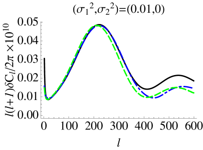
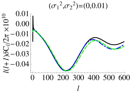
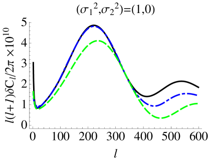
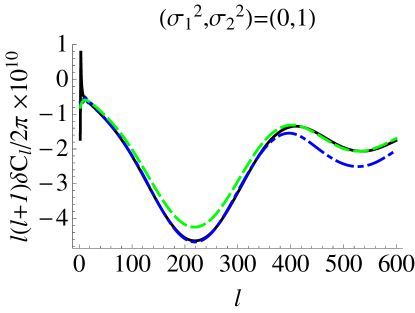
We can then find best-fit values of $\delta g_{i,\sigma_{j}^{2}}$. We perform a least-squares fit over the range $2\leq l\leq 600$, with weights given by the combination of cosmic variance and noise errors for WMAP. To test the validity of this procedure, we compute a new set of $C_{l}$’s using CMBFAST with parameters given by $\vec{g}^{(0)}+\delta\vec{g}$. Figure 4 shows that the fitting works very well, and that the linearity of the $C_{l}$’s in the specific direction of $\delta\vec{g}$ validates the approximation in equation (33). For $\sigma_{1},\sigma_{2}$ of order 1, linearity starts to break down, but such large values are probably unphysical in any case.

Numerically, in the linear regime the changes in parameters can be calculated by

$$\delta\vec{g}=\begin{pmatrix}\delta\Omega_{b}\\ \delta\Omega_{\rm cdm}\\ \delta\Omega_{\Lambda}\\ \delta n\\ \delta h\\ \delta A\end{pmatrix}\approx\begin{pmatrix}3.86\times 10^{-4}&0.963\times 10^{-4}\\ -6.33\times 10^{-3}&-5.78\times 10^{-3}\\ 5.24\times 10^{-3}&4.26\times 10^{-3}\\ -8.39\times 10^{-3}&-7.88\times 10^{-3}\\ 4.74\times 10^{-3}&6.55\times 10^{-3}\\ -0.285&-0.753\end{pmatrix}\begin{pmatrix}\sigma_{1}^{2}\\ \sigma_{2}^{2}\end{pmatrix}$$ (37)

In all cases except for the overall normalization $A$, the parameter changes are small even for relatively large $\sigma_{1}^{2},\sigma_{2}^{2}\sim 1$. Moreover, as can be seen in Figure 4, the residuals $\delta C_{l}$ have similar shape to the input power spectrum $C_{l}$ (although with a negative prefactor for $\sigma_{2}$), indicating that the chief error in the linear approximations in this section applies to the normalization. We conclude that, in a model of the form considered here, one should take care to recompute the overall normalization, which affects the normalization of the matter power spectrum, but that other parameters are likely to remain approximately unchanged.

VI Foregrounds

The significance of the observed anomalies depends on the choice of data set (e.g., Land and Magueijo (2007)). We chose to work in spherical harmonic space, leading to the requirement of an all-sky data set. We thus worked with the WMAP ILC data. With this choice of data set, one must wonder about the effect of residual foreground contamination on our results.

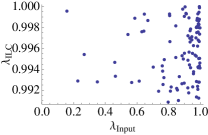
We can begin to assess these effects using a set of 10 000 publicly available ILC simulations Eriksen et al. (2005). For each simulation, both the foreground-free input map and the ILC reconstructions, with residual foreground contamination, are provided. In each case, we computed the four statistics discussed in this paper, namely the angular-momentum statistic $\lambda$, the Schwarz et al. multipole vector statistic $S$, the multipole vector alignment statistic $A$, and the planarity statistic $p$. Figure 5 shows a comparison of the input and and ILC maps for each statistic. In each case, there is a strong correlation, but the scatter is considerable.

The probability density for each of the four statistics undergoes no significant change between the input and ILC ensembles. (In other words, in each of the four plots on the top row of Figure 5, histograms of the $x$ and $y$ values look essentially identical.) This can be quantified in a variety of ways. Since we are most interested in the probability distribution near the upper tail of the distribution of each statistic (except for $p$, which has negligible effect on any of our conclusions anyway), we look at the behavior of the distributions near the 99th percentile. For each statistic, we find the 99th-percentile value in the 10 000 ILC maps, and count the number of input maps lying above that value. (The results are essentially identical if the two roles are reversed.) If the input and ILC probability densities are the same, we expect to find 100 in each case. The actual values found deviate from this expected value by $1,1,5,-6$ for $\lambda,S,A,p$ respectively. All are well within the $10\%$ fluctuation level expected due to Poisson noise.

From this test, we can conclude that foregrounds do not significantly alter the statistical significance of anomalies based on these statistics. Due to the problem of a posteriori statistics, reasonable people can disagree about whether to take the ILC multipole alignment seriously, but one’s opinion on this question need not be altered by consideration of foreground contamination.

In this paper we do not chiefly address the question of whether the multipole alignment is statistically significant; on the contrary, we provisionally adopt the stance that it is and ask what form an explanation of it might take. For this sort of question, we need to go beyond the simple considerations above and consider the correlations between input and ILC maps. After all, nonstandard cosmological models such as the broken-isotropy models we consider affect the probability of seeing multipole alignments in the foreground-free (“input”) maps, whereas the likelihoods that form the basis of our evidence calculations are based on the ILC map.

Once again, for the three statistics $\lambda,S,A$ that primarily affect our results, we are interested in the relation between input and ILC values near the upper end of the statistics’ ranges. Specifically, we want to know whether the observed large ILC value implies a large input value in the foreground-free CMB. The bottom row of plots in Figure 5 provides one qualitative way of addressing this question. For each statistic, we show a scatter plot comparing input and ILC values as in the upper row, but showing only points corresponding to the top 1% of ILC values. Many points cluster near the right, indicating that a high ILC value is likely, but by no means certain, to have come from a high input value.

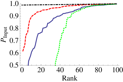
Let us be slightly more quantitative. For any given statistic, say $\lambda$, we extract the realizations for which the ILC maps are anomalously high, lying in the top 1% of the distribution. For these 100 realizations, we find the value of the statistic in the input map, $\lambda_{\rm Input}^{*}$, and look at its ranking in the full set of 10 000 input realizations. This gives the cumulative probability $P_{\rm input}\equiv{\rm Pr}[\lambda_{\rm Input}<\lambda_{\rm Input}^{*}]$ for each of the 100 input maps. If foreground contamination were negligible, then these 100 maps would lie in the top percentile of the input distribution, i.e., all 100 $P_{\rm input}$ values would be above 0.99.

Figure 6 shows the result of this exercise for each of the three statistics $\lambda,S,A$. In each case, the results are sorted by the value of the statistic in the input data. The results show that the statistic $S$ is least affected by foreground contamination: if a realization lies in the top 1% of the ILC maps, there is a high probability that it also lies near the top of the probability distribution of the input maps as well. For the three statistics $\lambda,S,A$, the median values of $P_{\rm Input}$ for the ILC top 1% maps are 93.2%, 98.5%, 89.0%, as compared to the value 99.5% that would occur if there were no foregrounds.

Generically, if the correlation between input and ILC maps is weak, then we would expect the enhanced likelihood and Bayesian evidence results of Section IV to be overestimates of the correct results. Intuitively, this seems clear: if the connection between the true CMB and the observed ILC data is weak, then so is our ability to draw cosmological conclusions from the ILC data. We can express this idea more formally as follows. Our theoretical models allow us to calculate probability distributions for the “input” data (i.e., the pure CMB), while our observations are of the ILC data. The correct procedure, therefore, is to convert the input probability distributions into ILC probability distributions by convolution with a conditional probability function $P({\rm ILC}|{\rm Input})$. Such a convolution would smooth out variations in likelihood.

We conclude, therefore, that because of foreground contamination, the results shown in Section IV should be regarded as upper limits. The effect of foregrounds on the results is difficult to quantify, but based on Figure 6 we expect it to be smallest for the results based on the Schwarz et al. statistic $S$.

Figure 6: For the three statistics $\lambda$ (solid), $S$ (dashed), $A$ (dotted), we select the top 1% of ILC simulations, and determine the cumulative probability $P_{\rm Input}$ of the statistic in the input map. The values are sorted and plotted. In the absence of any effect from foregrounds, ILC and input maps would be identical, and the result would be a straight line extending from 0.99 to 1 (dot-dashed line).

VII Discussion

The various anomalies that have been noted in the large-angle CMB may provide hints of departures from the standard cosmological model, possibly including violations of statistical isotropy. Although the statistical significance of these anomalies is difficult or even impossible to quantify a posteriori, these possibilities are exciting enough to warrant closer examination.

We have considered several classes of physically-motivated models that might explain the anomalies. We have calculated Bayesian evidence ratios to assess the degree to which the purported anomalies in the multipoles $l=2,3$ favor the anisotropic models over the standard model.

According to the pioneering work of Jeffreys Jeffreys (1961), a Bayesian evidence ratio constitutes “substantial” evidence if $\ln\Lambda>1$ and “strong” evidence if $\ln\Lambda>2.5$. As the results in the Section IV make clear (note that what is plotted in each case is $\Lambda$, not $\ln\Lambda$), only for the most judicious choice of prior do the tests performed here reach the “substantial” level, and they never come close to being “strong.”

Of course, Jeffreys’s criteria are somewhat arbitrary, but in this case they seem to describe the situation fairly well. Recall that the evidence ratio $\Lambda$ is simply the factor by which the ratio of prior probabilities must be adjusted, in the light of the observations, in order to get the posterior probability ratio. Presumably, the prior probability distribution assigns very low weight to the less natural anisotropic models, so even after applying an evidence ratio $\Lambda\sim 3$, the anisotropic models are still considered unlikely. One would require an exponentially large evidence ratio before assigning significant probability to the anisotropic models.

We used several different statistical approaches to to characterize the observed multipole alignment. Some ($\lambda,S$) are adopted from previous work, while others $(A,p)$ are of our own devising. In the latter case, we attempted to minimize (although not eliminate) the problem of a posteriori statistics by choosing a method blindly that seemed to us to naturally encapsulate the observed phenomena with minimal arbitrary choices. In any case, the general consistency of the results based on the different statistics indicates that the approach we have followed is robust.

We have estimated the changes in cosmological parameter estimates that would arise if the anisotropic models were shown to be correct. The chief effect of the modulation is on the estimate of the overall power spectrum normalization, which would of course have consequences for studies of large-scale structure. Our calculations are valid only if the modulation is applied to the CMB at all $l$-values measured by WMAP. If a more complicated model is correct (e.g. Hou et al. (2010)), in which only some scales are modulated, then the parameter changes would presumably be smaller.

We have used simulations of the ILC mapmaking process to evaluate the degree to which foreground contamination might affect our results. The statistic $S$ appears least affected by this problem: ILC maps with high values of $S$ are very likely to correspond to high values of $S$ in the intrinsic CMB. A thorough treatment of foregrounds in our analysis would generically reduce the (already modest) enhancements in the evidence ratio, so due to the effects of foregrounds our results can be regarded as upper limits.

In this paper, we have tentatively adopted the point of view that there are anomalies to be explained. Of course, one would greatly prefer to settle this question in a way that was not plagued by the problem of a posteriori statistics. To do this, we would require a new data set that probes similar scales to the large-angle CMB. All-sky polarization maps may provide some insight into these issues Frommert and Ensslin (2009); Dvorkin et al. (2008). Another possibility is to survey the “remote quadrupole” signal found in the polarization of CMB photons scattered in distant clusters Kamionkowski and Loeb (1997), which can be used to reconstruct information on gigaparsec-scale perturbations Bunn (2006); Abramo and Xavier (2007). Although gathering data on these scales is a difficult task, the potential for learning about the structure of the Universe on the largest observable scales makes it worth pursuing.

References

- Hinshaw et al. (2003) G. Hinshaw, D. N. Spergel, L. Verde, R. S. Hill, S. S. Meyer, C. Barnes, C. L. Bennett, M. Halpern, N. Jarosik, A. Kogut, et al., Astrophys. J. Supp. 148, 135 (2003), eprint arXiv:astro-ph/0302217.
- Bennett et al. (2003) C. L. Bennett, M. Halpern, G. Hinshaw, N. Jarosik, A. Kogut, M. Limon, S. S. Meyer, L. Page, D. N. Spergel, G. S. Tucker, et al., Astrophys. J. Supp. 148, 1 (2003), eprint arXiv:astro-ph/0302207.
- Hinshaw et al. (2007) G. Hinshaw, M. R. Nolta, C. L. Bennett, R. Bean, O. Doré, M. R. Greason, M. Halpern, R. S. Hill, N. Jarosik, A. Kogut, et al., Astrophys. J. Supp. 170, 288 (2007), eprint arXiv:astro-ph/0603451.
- Jarosik et al. (2010) N. Jarosik, C. L. Bennett, J. Dunkley, B. Gold, M. R. Greason, M. Halpern, R. S. Hill, G. Hinshaw, A. Kogut, E. Komatsu, et al., ArXiv e-prints (2010), eprint 1001.4744.
- Larson et al. (2010) D. Larson, J. Dunkley, G. Hinshaw, E. Komatsu, M. R. Nolta, C. L. Bennett, B. Gold, M. Halpern, R. S. Hill, N. Jarosik, et al., ArXiv e-prints (2010), eprint 1001.4635.
- Komatsu et al. (2010) E. Komatsu, K. M. Smith, J. Dunkley, C. L. Bennett, B. Gold, G. Hinshaw, N. Jarosik, D. Larson, M. R. Nolta, L. Page, et al., ArXiv e-prints (2010), eprint 1001.4538.
- Copi et al. (2007) C. J. Copi, D. Huterer, D. J. Schwarz, and G. D. Starkman, Phys. Rev. D 75, 023507 (2007), eprint arXiv:astro-ph/0605135.
- de Oliveira-Costa et al. (2004) A. de Oliveira-Costa, M. Tegmark, M. Zaldarriaga, and A. Hamilton, Phys. Rev. D 69, 063516 (2004), eprint arXiv:astro-ph/0307282.
- Copi et al. (2004) C. J. Copi, D. Huterer, and G. D. Starkman, Phys. Rev. D 70, 043515 (2004), eprint arXiv:astro-ph/0310511.
- Schwarz et al. (2004) D. J. Schwarz, G. D. Starkman, D. Huterer, and C. J. Copi, Physical Review Letters 93, 221301 (2004), eprint arXiv:astro-ph/0403353.
- Hajian (2007) A. Hajian, ArXiv Astrophysics e-prints (2007), eprint astro-ph/0702723.
- Eriksen et al. (2004a) H. K. Eriksen, F. K. Hansen, A. J. Banday, K. M. Górski, and P. B. Lilje, Astrophys. J. 605, 14 (2004a).
- Freeman et al. (2006) P. E. Freeman, C. R. Genovese, C. J. Miller, R. C. Nichol, and L. Wasserman, Astrophys. J. 638, 1 (2006), eprint arXiv:astro-ph/0510406.
- Hansen et al. (2009) F. K. Hansen, A. J. Banday, K. M. Górski, H. K. Eriksen, and P. B. Lilje, Astrophys. J. 704, 1448 (2009), eprint 0812.3795.
- Hanson et al. (2010) D. Hanson, A. Lewis, and A. Challinor, ArXiv e-prints (2010), eprint 1003.0198.
- Bennett et al. (2010) C. L. Bennett, R. S. Hill, G. Hinshaw, D. Larson, K. M. Smith, J. Dunkley, B. Gold, M. Halpern, N. Jarosik, A. Kogut, et al., ArXiv e-prints (2010), eprint 1001.4758.
- Gordon et al. (2005) C. Gordon, W. Hu, D. Huterer, and T. Crawford, Phys. Rev. D 72, 103002 (2005), eprint arXiv:astro-ph/0509301.
- Bunn and Bourdon (2008) E. F. Bunn and A. Bourdon, Phys. Rev. D 78, 123509 (2008), eprint 0808.0341.
- Ackerman et al. (2007) L. Ackerman, S. M. Carroll, and M. B. Wise, Phys. Rev. D 75, 083502 (2007), eprint arXiv:astro-ph/0701357.
- Böhmer and Mota (2008) C. G. Böhmer and D. F. Mota, Physics Letters B 663, 168 (2008), eprint 0710.2003.
- Himmetoglu et al. (2009) B. Himmetoglu, C. R. Contaldi, and M. Peloso, Phys. Rev. D 79, 063517 (2009), eprint 0812.1231.
- Hinshaw et al. (2008) G. Hinshaw, J. L. Weiland, R. S. Hill, N. Odegard, D. Larson, C. L. Bennett, J. Dunkley, B. Gold, M. R. Greason, N. Jarosik, et al., ArXiv e-prints 803 (2008), eprint 0803.0732.
- Eriksen et al. (2004b) H. K. Eriksen, A. J. Banday, K. M. Górski, and P. B. Lilje, Astrophys. J. 612, 633 (2004b), eprint arXiv:astro-ph/0403098.
- Eriksen et al. (2005) H. K. Eriksen, A. J. Banday, K. M. Gorski, and P. B. Lilje, ArXiv Astrophysics e-prints (2005), eprint arXiv:astro-ph/0508196.
- Land and Magueijo (2007) K. Land and J. Magueijo, M.N.R.A.S. 378, 153 (2007), eprint arXiv:astro-ph/0611518.
- Eriksen et al. (2007) H. K. Eriksen, A. J. Banday, K. M. Górski, F. K. Hansen, and P. B. Lilje, Astrophys. J. Lett. 660, L81 (2007), eprint arXiv:astro-ph/0701089.
- Hoftuft et al. (2009) J. Hoftuft, H. K. Eriksen, A. J. Banday, K. M. Górski, F. K. Hansen, and P. B. Lilje, Astrophys. J. 699, 985 (2009), eprint 0903.1229.
- Marshall et al. (2006) P. Marshall, N. Rajguru, and A. Slosar, Phys. Rev. D 73, 067302 (2006), eprint arXiv:astro-ph/0412535.
- Liddle et al. (2006) A. Liddle, P. Mukherjee, and D. Parkinson, Astronomy and Geophysics 47, 040000 (2006).
- Liddle (2007) A. R. Liddle, M.N.R.A.S. 377, L74 (2007), eprint arXiv:astro-ph/0701113.
- Efstathiou (2008) G. Efstathiou, M.N.R.A.S. 388, 1314 (2008), eprint 0802.3185.
- Seljak and Zaldarriaga (1996) U. Seljak and M. Zaldarriaga, Astrophys. J. 469, 437 (1996), eprint arXiv:astro-ph/9603033.
- Zare (1988) R. N. Zare, Angular Momentum: Understanding Spatial Aspects in Chemistry and Physics (Wiley, 1988).
- Tegmark et al. (2003) M. Tegmark, A. de Oliveira-Costa, and A. J. Hamilton, Phys. Rev. D 68, 123523 (2003), eprint arXiv:astro-ph/0302496.
- Jeffreys (1961) H. Jeffreys, Theory of Probability (Oxford University Press, 1961).
- Hou et al. (2010) Z. Hou, A. J. Banday, K. M. Górski, N. E. Groeneboom, and H. K. Eriksen, M.N.R.A.S. 401, 2379 (2010), eprint 0910.3445.
- Frommert and Ensslin (2009) M. Frommert and T. A. Ensslin, ArXiv e-prints (2009), eprint 0908.0453.
- Dvorkin et al. (2008) C. Dvorkin, H. V. Peiris, and W. Hu, Phys. Rev. D 77, 063008 (2008), eprint 0711.2321.
- Kamionkowski and Loeb (1997) M. Kamionkowski and A. Loeb, Phys. Rev. D 56, 4511 (1997), eprint arXiv:astro-ph/9703118.
- Bunn (2006) E. F. Bunn, Phys. Rev. D 73, 123517 (2006), eprint arXiv:astro-ph/0603271.
- Abramo and Xavier (2007) L. R. Abramo and H. S. Xavier, Phys. Rev. D 75, 101302 (2007), eprint arXiv:astro-ph/0612193.