Return distributions in dog-flea model revisited

Abstract

A recent study of coherent noise model for the system size independent case provides an exact relation between the exponent $\tau$ of avalanche size distribution and the $q$ value of the appropriate $q$-Gaussian that fits the return distribution of the model. This relation is applied to Ehrenfest’s historical dog-flea model by treating the fluctuations around the thermal equilibrium as avalanches. We provide a clear numerical evidence that the relation between the exponent $\tau$ of fluctuation length distribution and the $q$ value of the appropriate $q$-Gaussian obeys this exact relation when the system size is large enough. This allows us to determine the value of $q$-parameter a priori from one of the well known exponents of such dynamical systems. Furthermore, it is shown that the return distribution in dog-flea model gradually approaches to $q$-Gaussian as the system size increases and this tendency can be analyzed by a well defined analytical expression.

1 Introduction

Since the pioneering work of Bak, Tang, and Wiesenfeld (BTW) in 1987 [1], the self-organized criticality (SOC) paradigm has seen a burst of activity in the literature. In their seminal paper, by making use of so-called BTW sandpile model, these authors demonstrated that systems under their natural evolution are driven at a very slow rate until one of their elements reaches a critical stationary state and this triggers a sudden activity, i.e., avalanche. When the avalanche is over, the system evolves again according to the slow drive until a next avalanche is triggered without having any fine-tuning of parameters. Such a dynamic gives rise to the power-law correlations seen in the non-equilibrium steady states [2, 3].

Following the BTW sandpile model a great variety of models ranging from the deterministic and stochastic to the dissipative and conservative ones have been introduced which exhibit the phenomenon of SOC (for an overview, see [4] and references therein). Among them, a random neighbor version of the BTW sandpile model shows that a dynamical system with only two degrees of freedom can exhibit SOC and the dynamics can be described by a master equation [5]. Soon after the random neighbor BTW sandpile model was introduced, its conservative variant has been reported [6, 7]. This conservative variant is neither extended nor dissipative with regard to the amount of sand in the system but still shows SOC with critical exponents where the dynamics of the model is given by a Fokker-Planck equation. The avalanche size distribution $P(\lambda)$ is readily obtained by solving the Fokker-Planck equation at an absorbing boundary and is shown to exhibit a power-law regime $P(\lambda)\sim\lambda^{-\tau}$, followed by an exponential tail. Indeed, this model is an adaptation of the famous dog-flea model introduced by Ehrenfest in 1907 [8] to describe the process of approaching an equilibrium state in a large set of uncoupled two state systems in the presence of fluctuations (avalanches) around this state [9, 10].

In a recent work, the SOC feature of the dog-flea model was studied by simulating the underlying stochastic process that describes the natural evolution of the model [11]. In this paper, we show that the relation between the power-law exponent $\tau$ of the fluctuation length distribution and the $q$ value of the appropriate $q$-Gaussian that fits the return distribution (i.e., distribution of fluctuation length differences at subsequent time steps) obeys the rule

$$q=e^{1.19\tau^{-0.795}},$$ (1)

which was reported for the limited number of earthquakes from the World and California catalogs [12]. This approximate relation (1) enables one to obtain the value of $q$ parameter a priori from the power-law exponent $\tau$ of fluctuation length distribution. Using the same line of thought, the $\tau$ value for the dog-flea model was obtained as $\tau\simeq 1.517$ by making use of the maximum likelihood estimation method yielding to a value of $q=2.35$ of the concomitant $q$-Gaussian that fits the return distribution at $N\rightarrow\infty$ limit [11].

Soon after the relation (1) was reported, an exact relation between $\tau$ and $q$ has been introduced for the coherent noise model (CNM) in the size independent case as [13],

$$q=\frac{\tau+2}{\tau}.$$ (2)

These relations between $\tau$ and $q$ given by Eqs. (1) and (2) are slightly different from one another. Both relations approach $q=1$ at $\tau\rightarrow\infty$ limit while only the latter achieves the value $q=3$ for the given $\tau=1$ value [13]. Let us also remark that if we identify $\tau=1/(q_{s}-1)$, we can obtain from Eq. (2) $q_{s}-1=(q-1)/2$, which is precisely Eq. (30) in Ref.[14].

The chosen system size plays a crucial role in analyzing the SOC feature of the model. At relatively small system sizes, the distribution of the fluctuation length time-series $\lambda(t)$ in dog-flea model exhibits a power-law regime, which is followed by an exponential decay because of the finite size effects, while at large system sizes, the power-law regime increases and the exponential decay is postponed [11]. This size dependent behavior of the fluctuation length distributions results in different topological properties of the return distributions as we discuss in subsequent sections.

Our main task will be to analyze the SOC in the dog-flea model through numerical evaluation of the underlying stochastic process. In this manner the fluctuation length and return distributions are studied when the system size is large enough, i.e., at the $N\rightarrow\infty$ limit, and for small system sizes (i.e., when the finite size effects are visible). The rest of the paper is organized as follows. The model and the numerical procedure that we implement are given in the next section. Then, the probability distribution of fluctuation length for the system size, chosen so that the finite size effects are avoided, is obtained by numerical evaluations. Once the power-law exponent $\tau$ of the fluctuation length distribution is found, the distribution of returns are analyzed. Next, we analyze the return distribution of the dog-flea model when the finite size effects are visible. A summary and discussion of the results conclude this communication.

2 Dog-flea model

The dynamics of the dog-flea model has simple rules. The model has $N$ dynamical sites represented by the total number of fleas shared by two dogs (dog $A$ and dog $B$). Suppose that there are $N_{A}$ fleas on dog $A$ and $N_{B}$ fleas on dog $B$ leading to a population of fleas $N=N_{A}+N_{B}$. For convenience, $N$ is assumed to be even. In every time step, a randomly chosen flea jumps from one dog to the other. Thus, we have $N_{A}\rightarrow N_{A}\pm 1$ and $N_{B}\rightarrow N_{B}\mp 1$. The procedure is repeated for an arbitrary number of times. In the long time run, the mean number of fleas on both dog $A$ and dog $B$ converges to the equilibrium value, $\langle N_{A}\rangle=\langle N_{B}\rangle=N/2$ with the fluctuations around these mean values. A single fluctuation is described as a process that starts once the number of fleas on one of the dogs becomes larger (or smaller) than the equilibrium value $N/2$ and stops when it gets back to the value $N/2$ for the first time. Thus, the end of one fluctuation specifies the start of the subsequent one. The length ($\lambda$) of a fluctuation is determined by the number of time steps elapsed until the fluctuation ends.

Figure 1: (Color online) (a) Fluctuation length distribution for $N=10^{6}$. The full black line represents the fitting curve of the distribution with slope $\tau\simeq 1.517$. The distribution has an arbitrary normalization such that $P(\lambda=1)=1$. (b) Return distribution for $N=10^{6}$. The full black curve represents the appropriate $q$-Gaussian with $q=2.32$ determined from relation (2) a priori and $\beta=30$. The central part of the distribution is emphasized in the inset.

3 Fluctuation length and return distributions

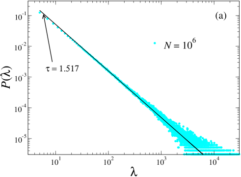
In order to study the behavior of return distributions with large $N$ the system size is chosen as $N=10^{6}$, enabling the finite size effects to appear only at very large fluctuation lengths. In Fig. 1(a), we plot the distribution of the fluctuation length time-series $\lambda(t)$ obtained from $2\times 10^{9}$ fluctuations. It can then be seen that the fluctuation length distribution follows a power-law regime, $P(\lambda)\sim\lambda^{\tau}$ with $\tau\simeq 1.517$ and exponential decay (i.e., finite size effects) is not visible.

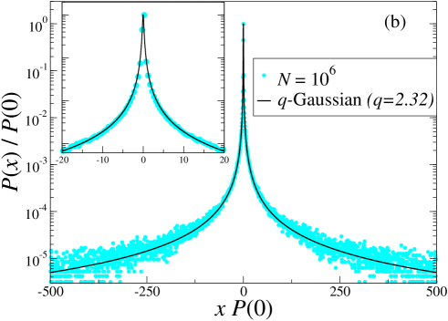
In Fig. 1(b), the distribution of returns, i.e., the difference between fluctuation lengths obtained at consecutive time steps, as $\Delta\lambda(t)=\lambda(t+1)-\lambda(t)$ is shown. At this point it should be emphasized that in order to have zero mean, the returns are normalized by introducing the variable $x$ as $x=\Delta\lambda-\langle\Delta\lambda\rangle$, where $\langle\cdots\rangle$ stands for the mean value of the given data set. From Fig. 1(b), it is clear that the signal of return distribution for $N=10^{6}$ is not Gaussian. Instead, it exhibits fat tails which is described by $q$-Gaussian,

$$P(x)=P(0)[(1+\bar{\beta}(q-1)x^{2}]^{1/(1-q)},$$ (3)

where $\bar{\beta}$ characterizes the width of the distribution and $q$ is the index of nonextensive statistical mechanics [15, 16]. As suggested in [13], the parameter $q$ can be determined directly from the relation (2) a priori as $q=2.32$. In Fig. 1(b), the solid black line represents the appropriate $q$-Gaussian with $q=2.32$ and $\beta=30$ that perfectly fits the signal of return distribution not only for the tails but for the intermediate and the very central part (see inset).

Figure 2: (Color online) (a) Fluctuation length distributions for $N=10^{2}$, $N=10^{3}$, $N=5\times 10^{3}$ and $N=10^{4}$. $10^{9}$ fluctuations are considered for each different system sizes. The legends of figure give the corresponding slope values $\tau$ of power-law regimes. The distributions have an arbitrary normalization such that $P(\lambda=1)=1$. (b) Return distributions for $N=10^{2}$, $N=10^{3}$, $N=5\times 10^{3}$ and $N=10^{4}$. The black lines on each return distribution represent the fitting curves obtained by Eq. (4) with $q$ values determined a priori from the relation (2) using the corresponding $\tau$ values. For each curve $a_{q}=30$ which is equal to $\beta$ value of appropriate $q$-Gaussian that fits the return distribution with largest system size, i.e., $N=10^{6}$. In the inset, we also give the parameter $a_{1}$ as a function of $N$ in order to better visualize how the finite-size effect disappears as $N$ increases. It is clear that $a_{1}$ appears to vanish as $a_{1}=963N^{-2}$.

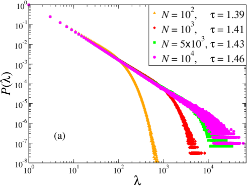
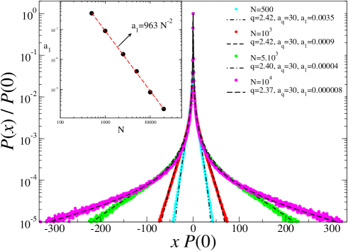
The fluctuation length distribution $P(\lambda)$ in dog-flea model shows size dependent behavior. Its signal exhibits a power-law regime following by an exponential regime because of finite-size effect at relatively small system sizes. However, as it has been reported in [11], the finite-size scaling hypothesis is satisfied. In Fig. 2(a), the fluctuation length distribution of $10^{9}$ fluctuations for four different system sizes $N=10^{2}$, $N=10^{3}$, $N=5\times 10^{3}$ and $N=10^{4}$ are presented. As the system size increases the power-law regime gets longer and the exponential decay is postponed. Since the system size is far away from being at the $N\rightarrow\infty$ limit (i.e., not large enough to avoid the finite size effects), each distribution of fluctuation length has different power-law slopes with slightly different $\tau$ values. This difference between the $\tau$ values of each distribution of fluctuations for different system sizes leads to return distributions, which are neither Gaussian nor $q$-Gaussian. Nevertheless, from Fig. 2(b) it is obvious that as the system size $N$ increases, leading to a longer power-law regime in the fluctuation length distribution, the curves of return distributions start to exhibit a tendency to a kind of fat tailed distribution, i.e., $q$-Gaussian. This gradual approach to $q$-Gaussian in the presence of finite-size effect is described by the following distribution [16, 17, 18],

$$y=\left[1-\frac{a_{q}}{a_{1}}+\frac{a_{q}}{a_{1}}e^{(q-1)a_{1}x^{2}}\right]^{1/(1-q)}.$$ (4)

If $a_{1}=0$, Eq. (4) coincides with the $q$-Gaussian and a Gaussian is recovered for $a_{q}=a_{1}$ (i.e., $q=1$).

As it is the case in CNM [13], Eq. (4) seems to coincide with the signal of the return distribution when the finite-size effects are invisible in dog-flea model. As it is seen from Fig. 2(b), each return distribution corresponding to different system sizes exhibits a topological behavior which is fitted by Eq. (4) with appropriate $q$ values determined a priori from the relation (2). Each critical exponent $\tau$ for different system sizes is obtained by considering only the power-law regime of corresponding fluctuation length distribution, see Fig. 2(a). Fig. 2(b) also reveals the fact that the longer the power-law regime persists for fluctuation length distribution, the better the appropriate $q$-Gaussian dominates in the return distribution. Eventually, as $N\rightarrow\infty$, the power-law regime of fluctuation length distribution is expected to continue forever (see Fig. 1(a)). It is also evident from the inset of Fig. 2(b) that the finite-size effects vanish as $N^{-2}$, which is completely the same tendency found in [13] for the coherent noise model. When the finite-size effects disappear, the corresponding return distribution seems to converge to the $q$-Gaussian for the entire region (see Fig. 1(b)).

4 Conclusion

We analyze the SOC in Ehrenfest’s dog-flea model through the probability distributions of fluctuation length and of the differences between the fluctuation lengths at subsequent time steps, i.e., returns, by simulating the stochastic process that describes the evolution of model. The fluctuations around the thermal equilibrium are treated as avalanches. In order to avoid the finite-size effects the size of the system is chosen large enough, i.e., $N=10^{6}$. This enables one to obtain a power-law regime with slope $\tau\simeq 1.517$ without any exponential decay. Then, the signal of return distribution is analyzed and it is shown that it converges to a $q$-Gaussian with $q=2.32$, a value obtained a priori from Eq. (2). This $q$ value is slightly different from the one reported in [11], where $q=2.35$ has been obtained using Eq. (1). The difference between the $q$ values for the same distribution stems from the fact that Eq. (1) is an approximate relation slightly differing from the exact relation given by Eq. (2) (see [13] for details).

The case where the finite-size effects are visible is also investigated by extensive simulations. When the system size is chosen relatively small, the finite-size effects appear in the avalanche size distribution: the distribution follows a power-law regime with corresponding slope value $\tau$ followed by an exponential decay. In this case, the return distributions numerically converge to appropriate $q$-Gaussian starting from the central part and gradually evolves towards the tails as the system size increases. This behavior of return distribution is indeed in good agreement with the one obtained when the system size is large enough. It is also found that the finite-size effects vanish as $N^{-2}$. As $N\rightarrow\infty$ the signal of return distributions for the finite system sizes numerically converges to a $q$-Gaussian in the entire region.

Acknowlegment

This work has been supported by TUBITAK (Turkish Agency) under the Research Project number 104T148 and by Ege University under the Research Project number 2009FEN027.

References

- [1] P. Bak, C. Tang, K. Wiesenfeld, Phys. Rev. Lett. 59 (1987) 381.
- [2] H. J. Jensen, Self-Organized Criticality: Emergent Complex Behavior in Physical and Biological Systems, Cambridge University Press, Cambridge, 1988.
- [3] P. Bak, How nature works: The science of self-organized criticality, Copernicus, New York, 1996.
- [4] D. Dhar, Physica A 369 (2006) 29.
- [5] H. Flyvbjerg, Phys. Rev. Lett. 76 (1996) 940.
- [6] J. Nagler, C. Hauert, H. G. Schuster, Phys. Rev. E 60 (1999) 2706.
- [7] C. Hauert, J. Nagler, H. G. Schuster, J. Stat. Phys. 116 (2004) 1453.
- [8] P. Ehrenfest, T. Ehrenfest, Phys. Z. 8 (1907) 311.
- [9] M. Kac, Am. Math. Monthly 54 (1947) 369.
- [10] N. Wax (Ed.), Selected papers on noise and stochastic processes, Dover, New York, 1954.
- [11] B. Bakar, U. Tirnakli, Phys. Rev. E 79 (2009) 040103(R).
- [12] F. Caruso, A. Pluchino, V. Latora, S. Vinciguerra, A. Rapisarda, Phys. Rev. E 75 (2007) 055101(R).
- [13] A. Celikoglu, U. Tirnakli, S. M. D. Queirós, arXiv: 1003.0361 [cond-mat.stat-mech] (2010).
- [14] C. Tsallis, A. R. Plastino, F. R. Alvarez-Estrada, J. Math. Phys. 50 (2009) 043303.
- [15] C. Tsallis, J. Stat. Phys. 52 (1988) 479.
- [16] C. Tsallis, Introduction to Nonextensive Statistical Mechanics - Approaching a Complex World, Springer, New York, 2009.
- [17] C. Tsallis, G. Bemski, R. S. Mendes, Phys. Lett. A 257 (1999) 93.
- [18] C. Tsallis, U. Tirnakli, J. Phys.: Conf. Ser. 201 (2010) 012001.