The Geometry of Nonparametric Filament Estimation
Abstract
We consider the problem of estimating filamentary structure from planar point process data. We make some connections with computational geometry and we develop nonparametric methods for estimating the filaments. We show that, under weak conditions, the filaments have a simple geometric representation as the medial axis of the data distribution’s support. Our methods convert an estimator of the support’s boundary into an estimator of the filaments. We also find the rates of convergence of our estimators.
keywords:
[class=AMS]keywords:
t1Thanks to Pierpaolo Brutti for pointing us to some useful references and Tony Cai for helpful comments. This research was partially supported by NSF grant DMS-08-060009. and
Contents
\@starttoctoc
1 Introduction
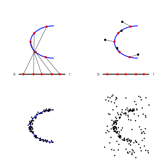
Filaments are one-dimensional curves embedded in where . Filament estimation has important applications in many fields including astronomy, geology, and medicine. Our basic filament model is
| (1) |
where . The unobserved variables are drawn from a distribution on and are drawn from a mean zero noise distribution . The goal is to estimate
| (2) |
Later, we extend the model to include background clutter, other ’s drawn uniformly from a compact set containing the filaments. See Figure 1. Estimating is an example of one-dimensional manifold learning. It may also be regarded as a type of principal curve estimation.
There is a plethora of available statistical methods that can, in principle, be used for estimating filaments. These include: principal curves (Hastie and Stuetzle (1989), Kegl et al. (2000), Sandilya and Kulkarni (2002), and Smola et al. (2001)); nonparametric, penalized, maximum likelihood (Tibshirani, 1992); beamlets (Donoho et al. (2001), and Arias-Castro et al. (2006)); parametric models (Stoica et al. (2007)); manifold learning techniques (Tenenbaum et al. (2000), Roweis and Saul (2000), and Huo and Chen (2002)); gradient based methods (Novikov et al. (2006), and Genovese et al. (2009) and methods from computational geometry (Dey (2006), Lee (1999), and Cheng et al. (2005)).
In this paper, we make some connections between the statistical problem and some ideas from computational geometry. We propose new, simple, nonparametric estimators for , and we find their rates of convergence. To the best of our knowledge, our methods are the first that are computationally simple, consistent, and have given rates of convergence with the exception of Cheng et al. (2005). However, our methods are simpler than those in Cheng et al. (2005), our assumptions are weaker, our loss function is more stringent and our estimators have faster rates of convergence.
The optimal rates of convergence for this problem appear to be unknown. In related work (Genovese et al. (2010)) we derived the minimax rate under stringent conditions. In ongoing work, we are finding the minimax rate under more general conditions. These rates depends critically on various features of the noise distribution . The methods in this paper are unlikely to be minimax optimal. Nonethless, they achieve reasonable rates of convergence and are simple to compute.
Our basic strategy involves two steps:
-
1.
Construct a set of fitted values that are close in Hausdorff distance to the filament.
-
2.
Extract a curve from this set of fitted values.
Motivation. The need to identify filamentary structures arises in a wide variety of applications. In medical imaging, for instance, filaments arise as networks of blood vessels in tissue and need to be identified and mapped. In remote sensing, river systems and road networks are common filamentary structures of critical importance (Lacoste et al. (2005); Stoica et al. (2004)). In seismology, the concentration of earthquake epicenters traces the filamentary network of fault lines. Filaments are of particular interest in astronomy because the distribution of galaxies in the universe is concentrated on a network of filaments that is often called the “cosmic web.” Indeed, astronomers have substantial literature on the problem of estimating filaments; see Luo and Vishniac (1995), van de Weygaert and Aragon-Calvo (2009), Martinez and Saar (2002), Barrow et al. (1985), Stoica et al. (2005), Eriksen et al. (2004), Novikov et al. (2006), Sousbie et al. (2006) and Stoica et al. (2007).
Summary of Results. Two key geometric ideas underlie our results – the medial axis of a set and the thickness of a curve – both of which are defined in Section 3. The medial axis is like the median of a set. The thickness of a curve measures both the curvature and how close the curve comes to being self-intersecting.
Our main results are the following:
-
1.
If the noise level of is less than the thickness , the filament equals the medial axis of the support of ’s distribution (Theorem 3).
-
2.
Any estimate of the boundary of the support of the distribution can be converted into an estimate of the filament that is close in Hausdorff distance to the true filament (Theorems 9 and 10). If the rate of convergence of the boundary estimator is then the rate of convergence of the filament estimator is also .
-
3.
Our estimators produce a set of fitted values that contain the filament and are close to it in Hausdorff distance. In Section 5, we show how to extract curves from the set estimators that are Hausdorff close to the true filament.
Proofs of all results are given in Section 6.1.
Notation. The boundary of a set is denoted by . The Hausdorff distance between two sets and is
| (3) |
where
| (4) |
denotes the -enlargement of the set , and denotes a closed ball centered at with radius . If is a set and is a point then we write . The closure of is denoted by and the complement of by . A curve is a map . Throughout, we use symbols like to denote generic positive constants whose value may be different in different expressions.
2 The Model
We will focus on finding filaments in a two dimensional point process although the ideas extend to higher dimensions. We begin with a single filament. Suppose we observe where
| (5) |
where , where is a distribution on and are drawn from .
Denote the graph of the filament by
| (6) |
With some abuse of terminology, we refer to both and as the filament. We assume that is contained in a compact set which, without loss of generality, we take to be .
The output of our algorithms will be a set which need not be a curve. Our loss function is Hausdorff distance
| (7) |
We will also show how to extract a curve from .
Next we define a smoothness condition for . For any three distinct points on let be the radius of the circle passing through the three points. Define the thickness of the curve , (Gonzalez and Maddocks, 1999) denoted , by
| (8) |
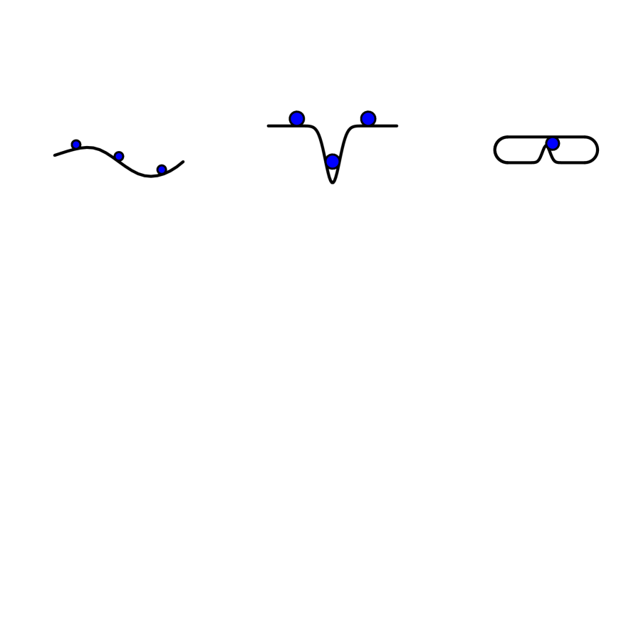
where the minimum is over all triples of distinct points on . is also called the minimum global radius of curvature, and the normal injectivity radius of and the condition number (Niyogi et al. (2008)). The thickness has the following interpretation: it is the minimum radius of all circles that are tangent to one point of while passing through another point of . A ball of radius tangent to a point on can contain points in other than . This can occur because the radius of curvature of is smaller than or because the curve comes within of self-intersecting. See Figure 2. Hence the thickness combines information about curvature and separation, capturing both local and global features of the curve. A useful way to think of is that it is the largest radius of a ball that can roll freely around .
If we say that is open. If we say that is closed. If, for , implies that then we say that is simple, or non-self-intersecting. Otherwise, we say it is self-intersecting. Unless stated otherwise, we assume that is smooth (non-zero, finite gradient at every point) and simple. We assume that the filament is parameterized with respect to arclength, normalized to .
We make the following assumptions:
- (A1)
-
has density with respect to Lebesgue measure on that is bounded and bounded away from zero:
(9) for some .
- (A2)
-
The noise distribution satisfies these conditions:
-
1.
has support .
-
2.
has bounded continuous density with respect to Lebesgue measure on and for all in the interior of .
-
3.
is nonincreasing, that is, implies that .
-
4.
is symmetric, i.e. implies that .
-
5.
There exists and such that
-
1.
- (A3)
-
is sufficienty smooth, i.e., . If is open, then also
.
The parameter controls the behavior of near the boundary of its support. The marginal density of is . Let
| (10) |
denote the support of . It follows from assumption (A2) that
| (11) |
We will let denote the distribution of the data corresponding to density . The boundary behavior of is related to . Let
| (12) |
Lemma 1
There exist constants such that the following is true. Let be in the interior of . For small enough we have that
| (13) |
We remark that if the noise density is uniform on , then and so is not uniform over its support. In fact, on .
Multiple filaments can be modeled by allowing to be piecewise continuous instead of continuous. Multiple filaments can also be represented as follows. Let be a set of one dimensional curves in where , . Let be a distribution on and let denote different distributions on . For let
We can also extend the model to allow for clutter, as in Gasgupta and Raftery (1998). Let denote a uniform distribution on a compact set and define the mixture where . We call points drawn from background clutter. Until Section 3.5, we will assume no clutter is present (i.e., ). Another generalization of the model is to allow to be self-intersecting, which we consider briefly later.
3 Estimation
It will be helpful to first make some connections with some concepts from computational geometry.
3.1 Some Backgound on Geometry
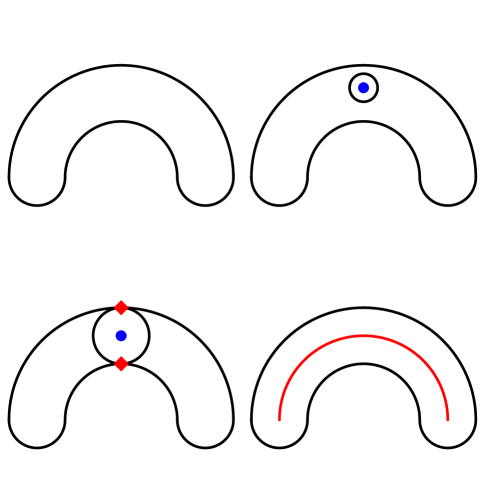
Let be a compact set. A ball is called medial if
-
1.
and
-
2.
contains at least 2 points.
The medial axis , shown in Figure 3, is the closure of the set
| (14) |
See Dey (2006) and references therein for more information about the properties of the medial axis.
For each let denote the normal vector at and the tangent vector at . Define the fiber,
| (15) |
and the tube
For open curves define the initial and final end caps, respectively, by
| (16) |
When is a closed curve, the end caps are empty, and when is open with ,
The next lemma gives a useful decomposition of the support set .
Lemma 2
-
1.
, and in particular, when is closed, .
-
2.
For every , and are disjoint.
-
3.
For every , there exists a unique fiber containing .
-
4.
For every , the closest point on to is either or .
-
5.
When is closed , when is open , where
and
are two non intersecting connected curves where and .
The following theorem relates the filament to its medial axis.
Theorem 3
-
1.
If is closed and then .
-
2.
If is open and then . If, in addition, then .
This result holds both good news and bad news. The good news is that , relating the filament to a well defined geometric quantity. The bad news is that the medial axis is not continuous in Hausdorff distance.

Small perturbations to give a completely different medial axis, as illustrated in Figure 4. Thus, estimating the medial axis is non-trivial. From now on, we assume that .
The Euclidean distance transform (EDT) (Breu et al. (1995)) is a mapping from defined by . The next result gives another characterization of the filament : the filament maximizes . In particular, .
Lemma 4
-
1.
if and only if .
-
2.
For any , .
-
3.
For any , .
Let be an estimate of and be an estimate of . For , define the empirical EDT by . We estimate the noise level by , where
| (17) |
Theorem 5
Suppose that . Then:
-
1.
.
-
2.
.
-
3.
.
Following Cuevas and Rodríguez-Casal (2004), we say that a set is -standard if there exist positive numbers and such that
| (18) |
where is Lebesgue measure. We say that is partly expandable if there exist and such that for all . (Recall that is the enlargement of ). A standard set has no sharp peaks while a partly expandable set has not deep inlets.
Lemma 6
is standard with and . Also, is partly expandable with and .
3.2 Estimating Boundaries
We estimate the support and its boundary . The estimate of will be converted into an estimator of the filament. The performance of these estimators, in Hausdorff-distance loss, translates directly to the performance of the filament estimators. We use to denote the rate of convergence of the boundary estimator; that is, .
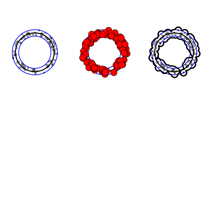
In practice, we will use the estimator from Cuevas and Rodríguez-Casal (2004) and Devroye and Wise (1980), described in the following result. An example is shown in Figure 5. This estimator is simple to use and fast to compute. Recall that where is defined in condition (A2).
Lemma 7
(Cuevas and Rodríguez-Casal (2004)). Let be a random sample from a distribution with support . Let be compact, -standard and partly expandable. Suppose the distribution has positive density and that for all , for some and some . Let
| (19) |
and let be the boundary of . If and then, with probability one
| (20) |
for all large , where . Also, almost surely for all large .
Proof Outline. The proof is essentially the same as the proof in Cuevas and Rodríguez-Casal (2004). They implicitly assume that . In particular their proof (see page 348 of their paper) argues that, for any , for some . This is true under standardness and assuming that . However, we allow to be 0 at the boundary and only require . In this case, by applying Lemma 1, we have that . The result then follows as in their proof by replacing with .
We will also need the following property of the union-of-balls estimator .
Lemma 8
Let be a sample from . If is open and if then is a simple, closed curve. If is closed and if then consists of two simple, closed curves and .
3.3 From Boundaries to Filaments
We now give two estimators of which we call the EDT estimator and the medial estimator. By condition (A3), so that .
The first estimator is inspired by the fact that the maximizes the EDT. The second estimator is inspired by the following fact. For a closed curve, consists of two disjoint pieces and and the medial axis is midway between and .
The algorithm for the EDT estimator is as follows. An example is shown in Figure 6.
The EDT Estimator
Input: support and boundary estimates and and a radius .
Output: a set of fitted values .
Algorithm:
-
1.
Compute , for all
-
2.
Set .
-
3.
Let and set .
We remark that the choice in the EDT procedure is mainly for theoretical purposes. In practice, can be used as a tuning parameter.
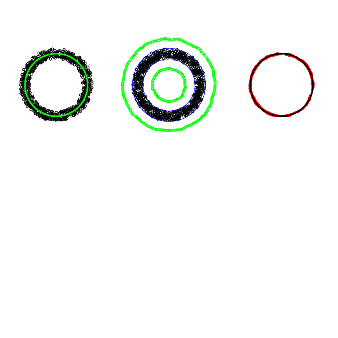
Theorem 9
Let be the EDT estimator, where .
-
1.
If , then , and .
-
2.
If where , and , then, with probability one,
(21) for all large , where .
Now we consider the medial estimator. In this case, we estimate the fibers by joining points on opposite sides of the estimated boundary. The algorithm for constructing the medial estimator follows:
The Medial Estimator
Input: support and boundary estimates and , where consists of two, disjoint curves and .
Output: a set of fitted values .
Algorithm:
-
1.
For each , let be the closest point on and let be the line segment connecting and .
-
2.
Set to be the midpoint of .
-
3.
Set .
We will focus on analyzing this algorithm for closed curves. The case of open curves is discussed in Section 6.2.
Theorem 10
Let be the medial estimator. Then:
-
1.
If and , with , then
-
(i)
For every there is a filament point such that .
-
(ii)
There exists such that, for each there is such that .
-
(iii)
.
-
(i)
-
2.
If where , and , then, with probability one, for all large ,
(22) where .
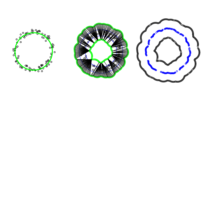
An example is in Figure 7. The medial estimator has a slower rate of convergence than the EDT estimator. However, Lemma 11 and Theorem 12 below show that it is easy to extract a curve from the fitted values. The extracted curve has the faster rate rather than .
Let be the medial estimator and assume that is closed. (The case where is open is considered in Subsection 6.2.) The fitted values are derived from the estimated boundary . These fitted values have gaps. All we have to do is connect the gaps with straight lines to get a curve. Surprisingly, this also improves the rate of convergence. Here are the details.
Recall that, from Lemma 8, and that is a closed simple curve. The medial estimator takes each point and outputs a fitted value . Let be a parameterization of , so . Define .
Lemma 11
The function is a union of open curves. In particular, there exist such that is a continuous, open curve on each but is possibly discontinuous at each .
Now we define as follows. In general, . We define to be the curve obtained by joining and by linear interpolation. We call the completed medial estimator.
Theorem 12
is a simple, closed curve. Furthermore, .
Multiple Filaments. Suppose now that there are finitely many filaments . First suppose that for all where . The properties of guarantee that for large enough , will consist of disjoint, connected sets .
Corollary 13
Suppose that , where denotes the thickness of the curve , and that for all . If the EDT or medial procedure is applied then
where is as before.
When the condition fails, then the curves can get close to each other or even could be self-intersecting. In that case, we cannot claim to estimate the entire curve well. However, we can estimate the well-separated portions of the curves. Let . For each let . Let .
Corollary 14
Suppose that . If either the EDT or medial procedures are applied then
where for the EDT estimator and for the medial estimator.
3.4 Extracting a curve from EDT estimator
Now we discuss how to extract a curve from the fitted values. We assume that we have already computed the union of balls estimator with an appropriate choice of and hence that and for some .
Let denote the fitted values from the EDT estimator. Our goal is to use to find a curve such . Such a curve can be identified both for open and closed filaments. The precise statement is given in Theorem 15 below.
More informally, recall first that from Theorem 9, . Now, when is an open filament, from Lemma 2, . Thus, let and be points in and the two end-caps of . Any curve between and that lies entirely in must cut through every fiber in at a distance at most and it is at most from the end points and . Hence .
When, instead, is a closed filament, let be a point in surrounded by . Any closed curve that lies entirely within and has winding number with respect to cuts through every fiber in at a distance at most from . In this case too .
The extraction algorithm is based on the remarks above. In the open filament case, because and are unknown, we replace and by estimated end-points and that maximize the minimum path length between two points in , as illustrated later in Subsection 6.3. In the closed filament case we use a slightly different implementation, that generalizes more readily to the case where it is not known if the filament is open or closed.
EDT Curve Extraction Algorithm
Input: EDT Estimate and corresponding , and constraint sets and . ( by default).
Output: the graph of a curve .
Algorithm (Open-Curve Case):
-
1.
Find end points and satisfying
(23) where is the set of paths in from to . In practice, this is accomplished by constructing a -net of points in with ; forming the minimum spanning tree of this net; and finding the points that maximize the minimum path length in the tree.
-
2.
Join the end points by a curve in . In practice, this is obtained from the minimum spanning via Dijkstra’s algorithm (Dijkstra (1959)).
-
3.
(Optional) Relax the path to thickness as follows: for each successive triple of points on the path, shrink as close to while remaining in . Iterate until the reduction in thickness is below a fixed threshold.
Algorithm (Closed-Curve Case):
-
1.
Fix .
-
2.
Let be the point defined in equation (17) that determines .
-
3.
Let be the union of all line segments through with end points on and whose length is .
-
4.
Define .
-
5.
Apply the open-curve algorithm to with the constraint that the end points of the curve, and , must both lie on (i.e., set ).
-
6.
Join and by a curve contained within , producing a single closed curve.
Algorithm (General-Curve Case):
-
1.
Construct as in the closed curve algorithm
-
2.
If has one connected component, continue with the closed-curve algorithm. (This can, for instance, be determined using a friends-of-friends with a threshold distance of from the closed-curve algorithm.)
-
3.
Otherwise, must have two connected components. Do the following:
-
(a)
Apply the open-curve algorithm to each component with the constraint that the one of the end points in each component must lie on the boundary of (i.e., and for the first component and vice versa for the second).
-
(b)
Join the endpoints on the boundary of with any path through to create a single curve.
-
(a)
For the open-curve case, specification of is arbitrary. Smaller give larger nets and lead more convoluted initial paths but allow more effective smoothing in the relaxation step. The minimum spanning tree end points can be refined by using the expected hitting times for a random walk on the -net. Restricting the random walk to suitably small steps of order gives a sparse transition matrix. The expected hitting time from one end point to all other points can be maximized to refine the other end point and so on, alternating end points. This process tends to converge rather quickly and produces better results in practice. Relaxation is optional but must be used if a smooth is desired.
For the closed curve case, the choice of is again arbitrary, a non-zero value is needed to provide clean separation. The set can be replaced in practice with the intersection of and a ball of radius around , which is easier to compute, if somewhat more conservative.
The following theorem shows that the algorithm produces curves with the desired properties.
Theorem 15
Let denote the curve extracted from the EDT estimator by the algorithm described above. Assume that . Then,
-
1.
If is closed, .
-
2.
If is open, .
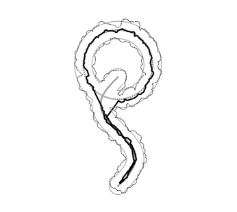
An example of curve extraction is shown in Figure 10.
3.5 Decluttering
Assume now that has density where is the uniform density over a compact set and is the density of points from the filament. We assume that where is the support of . Thus, where is the area of .
Let if is from and if is from . To identify clutter, we want to find a classifier where means that we guess that and means that we guess that .
The best classifier is the Bayes’ rule,
| (24) |
where
The Bayes rule is not identifiable. Since , a conservative approximation to the Bayes rule is
| (25) |
An estimate of is where is a density estimator obtained from . In practice we use a kernel density estimator. We can now apply the previous filament algorithms to the decluttered data set
| (26) |
An investigation into the properties of this decluttering process is beyond the scope of this paper and will be reported elsewhere. However, we will illustrate the decluttering procedure in the examples and show that it appears to perform well in practice.
4 Examples
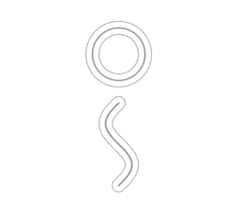
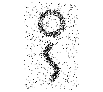
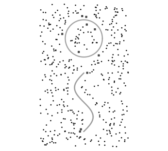
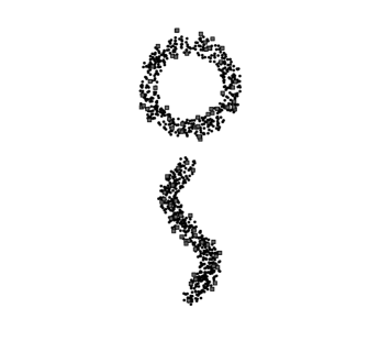
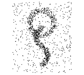
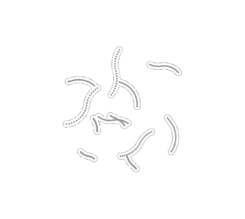
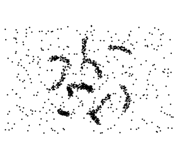
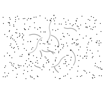
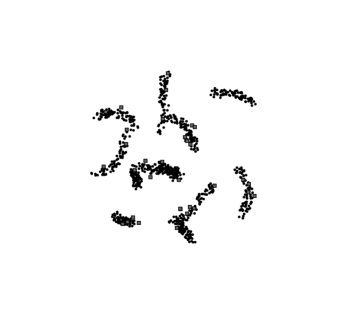
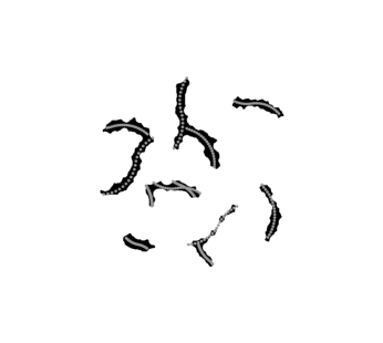
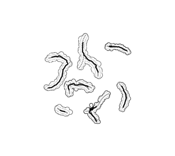
We have tested our procedures on a few simulated data-sets. We start by considering two smooth filaments, one open and the other closed. In the first example the two filaments are well separated (top left panel in Figure 9) while in the second dataset the two filaments intersect (top left panel in Figure 11). The third example considers 12 different smooth open filaments, with several intersections.
Note that the condition on the radius of curvature fails to hold in presence of intersections between filaments, thus only the first dataset satisfies the conditions of this paper completely.
In all the examples we have chosen according to the suggestion in Cuevas and Rodríguez-Casal (2004) as follows:
| (27) |
The first two datasets contain 1500 points: 500 of which on each filament and 500 points of background clutter (top right panels in Figures 9 and 11).
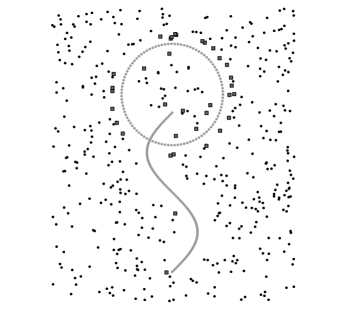
A summary of the results from the decluttering procedure is given in Figure 8 for both dataset. The procedure seems to work well in separating filament from clutter points.
| Marked as | |||
|---|---|---|---|
| True | filament | clutter | Total |
| filament | 990 | 10 | 1000 |
| clutter | 82 | 418 | 500 |
| Total | 1072 | 428 | 1500 |
| Marked as | |||
|---|---|---|---|
| True | filament | clutter | Total |
| filament | 965 | 35 | 1000 |
| clutter | 89 | 411 | 500 |
| Total | 1054 | 446 | 1500 |
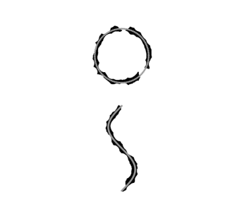
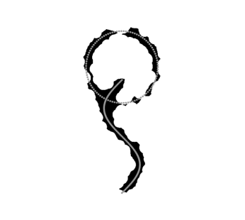
The filaments were estimated with the EDT and the Medial Estimator methods of subsection 3.3, applied to the decluttered datasets. The estimated filaments obtained for the first dataset are very close to the true (bottom panels in Figure 9).
 |
 |
 |
 |
 |
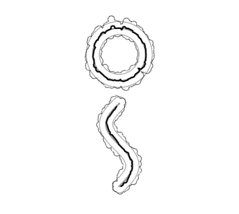 |
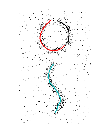
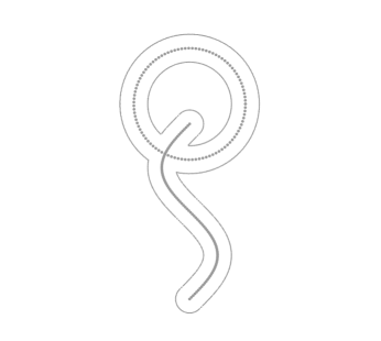
We applied the curve extraction procedure of subsection 3.4 to the EDT estimator shown in the bottom left panel of Figure 9. Figure 10 shows the extracted curves.
The estimated filaments obtained for the first dataset are very close to the true (bottom panels in Figure 9). For the second dataset (bottom panels in Figure 11) the medial estimator fails to detect the true filament near the intersection and becomes more and more accurate as it moves away from the intersection. Considering that the condition on the radius of curvature is violated, even in the second dataset the estimate seems to be quite satisfactory.
 |
 |
 |
 |
 |
 |
The third dataset is more challenging as it contains 12 filaments, with several intersections. Eighty points were generated from each filament and 350 more points were generated as background clutter, for a total of data points (top panels in Figure 12). The decluttering procedure (central panels in Figure 12) resulted in 989 points marked as filament (34 of which were generated as clutter) and 321 points marked as clutter (5 of which were filament points). The estimates, obtained from the points marked as filament, are shown in the bottom panel of Figure 12. These estimates are accurate for filaments with no intersections. The accuracy is less satisfactory for intersecting filaments or for filaments that are too close to each other. This was to be expected, as the condition on the radius of curvature is not satisfied in these cases.
 |
 |
 |
 |
 |
 |
5 Discussion
In recent work (Genovese et al. (2010)) we found the minimax rate for this problem under restrictive conditions (but in general dimensions). In current work, we are finding the minimax rates in general. This is a difficult problem because the rate depends critically on features of the noise distribution . Moreover, the problem is essentially a deconvolution problem since the variables are unobserved and corrupted by noise. We will report on these results elsewhere.
The estimators presented here are not minimax but are appealing because of their simplicity. Finding a practical estimator that achieves the minimax rate is an open question. Our approach, instead, consists of two steps: producing a set of fitted values and then extracting a curve from . We gave two specific methods for obtaining the fitted values and a curve extraction method for each of the two approaches. The resulting estimators have reasonably fast rates of convergence.
The noise model is critical. We assumed compact support which is reasonable for many applications. Without compact support, the behavior of the methods changes substantially as it does in nonparametric measurement error problems.
It is interesting to compare our results to those in Cheng et al. (2005). They show that each of their fitted values is from the filament. Under weaker conditions than they assumed, we get a rate which is faster as long as is not too large. (They implicitly assume that .) Also, our rate is in Hausdorff distance which is a stronger notion of closeness than used in their paper.
Currently, we are pursing several extensions of our results. These include: the aforemetioned extensions to higher dimensions (manifold learning), relaxing the smoothness condition, relaxing the constant condition, noise distributions with non-compact support and comparisons with beamlets. We are also investigating data-driven methods for choosing the tuning parameter and we are studying the theoretical properties of the decluttering technique.
6 Supplementary Material
6.1 Proofs
Let and let be the point on closest to . Without loss of generality, assume that and that the tangent vector to at is . We now prove that . In Lemma 2 we show that , where is defined in (15) as and is the normal vector at . Moreover, we show that the ’s are disjoint. Let such that , hence . Continuity of implies that there exists an interval such that for all in the interval. We will show later that . We can write the density at as and the conditional density
The denominator is bounded from above by . Hence,
Now we show that . Let , is bounded below by the distance of the intersection of the two balls and . Some algebra shows that
Finally, since
we obtain
It is easy to see that for all . Hence, .
Now we find the upper bound. Let . Let be such that . Now
Earlier we showed that . By a similar argument, for some . The result follows.
Proof of Lemma 2.
1. First, consider the closed case. We show that . Suppose not. Then there is a such that
for any and . Let be the closest point on the curve to . Since , . Without loss of generality, suppose that . So, for sufficiently small ,
which is a contradiction. For the open case, the balls and do not intersect. Both balls are contained in . The half plane formed by the normal vectors at and split these balls in two, with half of each in and half in . The result follows.
2. Now we show that implies that . Suppose that and intersect at some point . So
for some . Let be the ball of radius tangent to and containing . Let be the ball of radius tangent to and containing . Note that and . (This follows from the discussion after (8).) Now implies that but implies that and so . So, . By the triangle inequality,
But means that . So the inequality above must be equality which implies that , and fall on a line. Hence, and cannot intersect.
3. Follows directly from 2. because is the union of the fibers.
4. Follows from 1. and 5. follows from 4.
Proof of Theorem 3.
1. First we show that . Pick any . Let . We claim that contains at least two points. Let and . We will show that and are in .
Note that and hence they are in . In fact they are boundary points because they are not in the interior of . To show this, suppose to the contrary that is interior. Hence there exists such that . That is, is in the interior of . But this contradicts the assumption. The same argument shows that . Hence, and so .
Now we show that . Let . We claim that for some . Suppose not. From Lemma 2, for some and for any . Also, and contains and . Since and either or . Without loss of generality, assume that . Set and and note that . Let be the medial ball at . If then the interior of has nonempty intersection with . So must be less than or equal to . On the other hand, if then . So we must have . But is stricty contained in except for the common point . Thus, all points in are interior points of except for . So contains fewer that 2 points and hence cannot be in .
2. The proof that is the same as in part 1. Now suppose that . We will show that and hence . From Equations (15) and (16), recall that , , and denote the tube and the end caps. By Lemma 2, , where . Let . If then the proof of the previous part implies that for some . That is, . Now suppose . Then for some . We may assume otherwise is on the boundary and cannot be medial. Consider a ball . We claim that cannot be medial. In fact, if then all points in are interior to . If then intersects at a single point. Finally, if then . Thus cannot be medial and . Similarly, . Hence, .
Proof of Lemma 4. We prove the closed case. The open case is similar.
1. If then for some by Theorem 3. From lemma 2, the closest point on the boundary is either or . In either case, .
2. We have for some and . Since , it follows that and so . Then, from (1), .
3. We have for some and some . The closest boundary point is either or . Without loss of generality, assume it is . Hence, . So, .
Proof of Theorem 5.
1. Choose any . Let be the closest point to on . Let be the closest point to on . Let be the closest point to on . Then
Now let be the point on closest to . Then
2. Let and let be its closest point in . Then
Also
Proof of Lemma 6. Let be a point in and let be its distance from the boundary . If then so that .
Suppose that . Let be the point on the filament closest to and let be the point on the segment joining to such that . The ball is contained in both and . Hence, . This is true for all , hence is -standard for and .
Now we show that is expandable. By Proposition 1 in Cuevas and Rodríguez-Casal (2004) it suffices to show that a ball of radius rolls freely outside for some , meaning that, for each , there is an such that , where is the complement of . Let be the ball of radius tangent to such that . Such a ball exists by virtue of the conditions on .
Proof of Lemma 8. Suppose first that is open. Then is a closed, simple curve. Let . We will first show that is a closed, non-self-intersecting curve for all . Consider one observation and note that . Since , . It is then easy to see that is a closed, non-self-intersecting curve. A simple induction argument verifies that is a closed, non-self-intersecting curve for all . Now, when , we have and the conclusion follows. The proof for closed curves is similar.
Proof of Theorem 9.
1. First we show that implies that . Let . Then . So . Now we show that . Suppose that . Then,
so that .
2. The proof of the second statement follows from 1. and Lemma 7.
Lemma 16
Let and be two curves in such that . Given a point , let be the point on closest to . Let . Consider a ball, with radius and center , that contains , and no other points in . Then there exists a point such that and
| (29) |
Thus, .
Proof of Lemma 16. See Figure 13. Consider the ball with . Let be a point along the radius that joins with . Since , there exists a point within distance from , other than .
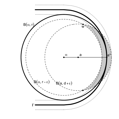
Note that , otherwise would be in , but, by construction, is the only point that belongs to . To show that , assume by contradiction that were in , then and
thus implying that .
Now, since , then , the shaded region in Figure 13. Thus, , where is either one of the two points where the two balls and cross in Figure 13.
Without loss of generality assume the system of coordinates is such that:
and the equation of the two balls are:
Thus the coordinates of are
and the distance between and
Lemma 17
Suppose . Let be the extended fiber. It can be shown that the extended fibers are disjoint. For a given let . Let be the point of () closest to . There exists such that and
| (30) |
with . Hence uniformly over .
Proof of Lemma 17. Let and note that . Consider two balls of radius tangent to the filament at on either side of . Both balls contain no points of other than . Let be the center of the ball on the side opposite to , so that is on the normal through .
Now we show that the balls , centered in satisfy the conditions required in Lemma 16. By construction, is tangent to at and . The center of is on the normal through , thus is the closest point to on the boundary and there are no other points in interior to the ball. Also cannot be tangent to the ball in a point , otherwise would be on the extended fiber for some . But the extended fibers are disjoint. This shows that is the ball of Lemma 16, with , and . Hence, from Lemma 16:
where . The result follows since , and .

1. Recall that and that for each we have .
(i) Let , and let and be the points that generated it, as in Figure 14. Let be the line segment that joins to . The distance between any and the boundary curves is, respectively, and . The midpoint on is such that and . Consider the point at the intersection between and .
To show that , and belongs to the ball in Figure 14, suppose to the contrary that , then either or . But if , then
which contadicts the fact that . If, instead , then
that contradicts the fact that .

(ii) Let , and let and be its closest points on and respectively, as in Figure 15. By construction, is on the midpoint of the segment , hence . Consider a point such that . Let and be the projections of on and respectively. The midpoint belongs to . From Lemma 17, uniformly. Moreover, from Lemma 19 that follows below, we have uniformly. Hence:
It follows that
(iii) is a consequence of (i) and (ii).
2. The second statement follows from statement 1. and Lemma 7.
Now we examine the two disjoint curves that constitute the boundary when is closed, and the set when is open. For each boundary curve we can distinguish two sides: one side that faces towards , and a second side that faces away from . Each point supports two tangent balls that contain no other points of , one on each side.
Analogously to the definition of thickness of a curve in Section 2, we define the Outer Thickness of the boundary to be the minimum radius of curvature of all the balls tangent to one point of on the side facing away from . We also define the Outer Critical Ball to be the ball facing away from and tangent to any point , with radius . Similarly, we define the Inner Thickness of the boundary to be the minimum radius of curvature of all the balls tangent to one point of on the side facing towards , and the Inner Critical Ball to be the ball facing towards and tangent to any point , with radius . Both balls can roll freely on the side of where they are constructed, but not necessarily on the other side. The thickness of the boundary curves is .
Lemma 18
For every point the outer critical ball has radius and the inner critical ball has radius . Thus the thickness of is .
Proof of Lemma 18. We start with the inner ball. Let be a point on the boundary . Hence, say. Let where . We claim that if is any other point on then . Let be the line segment connecting to . We wil show that the length of is strictly larger than . Now for some . The line crosses at some point . The closest point on to is and the distance from to is . Hence, . Let . Then and hence . Therefore, as required. The proof for the outer ball is similar.
Lemma 19
Let , and let be a second point in , such that . Denote by and , respectively, the projections of and on , then the distance between and is
Proof of Lemma 19. If then
If instead (see Figure 16), let be the center of the outer critical ball , and let be the angle . Consider the triangle with vertices in and . Since , from the law of sines applied to and to the angle facing
Now we show that the point , projected from onto , lies in the shaded region of Figure 16. In fact, the inner critical ball , tangent to is such that . Moreover, since is the closest point to , it follows that . Thus , and so , the shaded region in Figure 16. The two balls and intercept in the two points and .
Also, in the following Lemma 20, we show that implies that is the farthest point from in the shaded region.
The angle and the length of the chord is . Thus
Lemma 20
If then is the farthest point from in the shaded area of Figure 16.
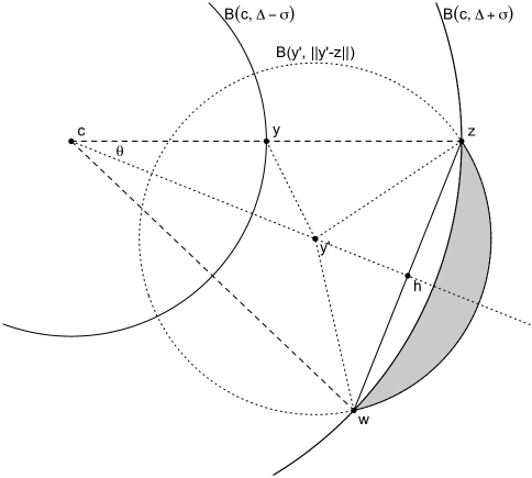
Proof of Lemma 20. See Figure 16. While keeping the angle fixed, and as long as , one can move the location of along the radius of from its center through . Let be the midpoint between and . If is chosen on the segment , then repeating the proof of Lemma 19 generates the same point as in Figure 16, and is still the point in the shaded region farthest away from .
If, instead, is chosen along the line from onwards, then, by construction, there are points in the shaded region that have distance from larger than . But such will violate the condition . In fact, assume without loss of generality that the system of coordinates is such that:
and the coordinates of and are
By construction, if lies along the line from onwards, then . This implies that , and
Proof of Lemma 11. This follows from the fact that and are each closed simple curves and that each consists of finitely many arcs of a circle.
Proof of Theorem 12. The fact that is a simple closed curve is straightforward. We have already shown that each fitted value is within distance of . It is easy to see that this is true of the linear completion as well. We still need to show that for each there is a fitted value with distance .
Choose any . The fiber divides into two disjoint sets. Let be the fitted value closest to from the first set and let be the fitted value closest to from the second set. Let . Let be the projection of onto and be the projection of onto . Let be the line connecting and . Since the endpoints of and are apart, it follows that .
There are two balls and of radius passing through and . The arc of the curve from and is contained in the lens . (If not, then a ball of radius could not roll freely.) So . But is simply the distance from the chord of a circle to the circle, where the chord has length . It follows that . Finally, .
Proof of Theorem 15. For the open-curve case with , claim 1. follows directly from Theorem 6.29. For the open-curve case with and , as used in the general variant of the algorithm, note that the endpoint in is a distance from , where is the corresponding component of . Moreover, every point in lies within of . Therefore 1. also follows from Theorem 6.29.
For the closed case, all that must be proved is that the estimated curve is a closed curve that lies within and that has (absolute) winding number 1 around a point in the inner component of . Notice also that in the closed case, both the closed and general variants of the algorithm produce the same curve.
First, recall that and notice that the unique fiber through , , intersects with in a line segment of length . This portion of a fiber is thus contained in the set (defined in EDT curve extraction algorithm for the closed curve case) and thus in ; in fact, the fibers for in an open set containing are also contained in . is thus cut at a fiber and contains a single connected component because . (If the latter were false, two separated parts of would lie within of each other.)
Second, applying the open curve algorith with produces a curve within that connects one side of to the other. (If the latter were false, the curve between the endpoints would have length , but a longer minimum path length can be obtained by winding around . The winding number cannot be greater than 1 because the curve in is not closed.) A path between these end points that is contained in closes this curve and keeps it within . The resulting closed curve thus lies within and has (absolute) winding number 1 with respect to . Claim 2. follows.
Lemma 21
Suppose is a compact, connected set in . Then,
-
1.
If and and if is the line segment from to , then
-
2.
Fix . If but , then .
Proof 6.22.
1. Define . We know that the infimum exists because is a compact set and that there is a unique point for which . It follows directly that every neighborhood of contains a point in and a point in , so .
2. Suppose the conclusion does not hold; that is, there exists a . By assumption, there is an . Apply Result 1 in the lemma to the line segment between and , which is contained in by convexity. This implies that , contradicting the initial supposition. The result follows.
6.2 Open Curves
This subsection deals with two issues related to open curves. First, the EDT curve extraction algorithm (Subsection 3.4) for open curves required that we estimate the endpoints of the curve. Second, for constructing the medial estimator in the open curve case, the estimated boundary needs to be split into two pieces and . Both issues are addressed here after the following discussion of some basic properies of open curves.
Let be an open curve and let the boundary support. Define
and
to be the extended end caps of the support’s boundary. Let, and . Define
Let denote the arclength of . Because is parameterized by arclength normalized to , it follows that the gradient of the filament is such that for all . Define
| (32) |
Theorem 6.23.
Let .
-
1.
and .
-
2.
Let . Then and .
-
3.
Let . Then and .
Proof 6.24.
(See Figure 17).
1. Let .
We will show that .
Note that cannot belong to hence, being ,
necessarily for some . We only need to
prove that .
Moreover, since for all
proving that would be sufficient for the claim.
We know that and that for some . The line from to defines the direction of the normal at . Extend the normal at to the point , so that and , hence must lie outside the circle . Let be the intersection between and the segment from to ; such intersection exixts because and . We have
where is positive.

Consider the triangle with vertices , and and denote by the angle at . The cosine theorem gives
so that
and
Now consider the triangle with vertices , and , where the angle at is . From the cosine theorem we obtain
And, since
Note that for small (as long as )
is a decreasing function of and then for all
As a consequence
and
3. Let . Then
6.3 Estimating the Endpoints
In this subsection we derive estimators for and . First we will need some lemmas. Let be the EDT estimator.
Lemma 6.25.
For fixed , the set has the following properties. Suppose and is the intersection of and the fiber of containing .
-
1.
If is closed, then is a connected line segment through .
-
2.
If is open and lies at least from and then is a connected line segment.
Proof 6.26.
Without loss of generality, we can assume that the fiber through is oriented vertically and that . must lie above the circle of radius centered on the origin, and thus the boundary of the support (on that side of ) must lie above the circle of radius centered on the origin. It follows that the outer portion of must lie above the circle of radius centered on the origin.
First, consider the point where for on the fiber through . Let for some and . And let . We want to find the maximum such that ; this will show limit the range of closest points.
We have that
Taking yields
Hence,
| (33) | ||||
| (34) |
and thus .
Second, consider a wedge of half angle around the vertical axis. Consider points and where and with . Let for and . We want to find the value of such that for all such . In this wedge, in other words, distance to the estimated boundary is monotone along the filament.
We have
Hence, requires that
or equivalently
This is satisfied whenever or equivalently when .
Combining these two parts, we see that the closest point to the boundary must lie within a wedge of angular extend , which is contained in the wedge for which distance to the estimated boundary is monotone along the filament. Claim 1. follows. For open curves, claim 2. follows from the same argument for a point for which the fiber through is sufficiently far from the endcaps.
Lemma 6.27.
has a finite piecewise (two continuous derivatives) boundary.
Proof 6.28.
Because , it is sufficient to show that has a piecewise smooth boundary. Since consists of all points such that for some constant , it follows that
| (35) |
Thus, consists of the points in that are exactly away from . Because is a finite union of circular arcs of radius , it follows that () is the boundary of a finite union of -enlargements of circular arcs. A set that is a finite union of sets with piecewise smooth boundaries itself must have a piecewise smooth boundary. Thus, it is sufficient to show that the -enlargement of a single circular arc has a piecewise smooth boundary.
To do this, let be a circular arc, which we can take without loss of generality to be of the form
for . Let and be the two endpoints. Let denote the point(s) in that is (are) closest to . For in the cone for , . For on the negative horizontal axis, contains the two endpoints of the arc. For all other , contains the endpoint of the arc on the same side of the horizontal axis as . It follows that the set of points for which is a union of three circular arcs: one in the cone consisting of points at radius , one for consisting of part of the circle around , and one for consisting of part of the circle around . This proves the lemma.
Theorem 6.29.
Let be an open curve. Let denote the set of paths between that are contained in . Define by
| (36) |
where length denotes the arclength of the path.
Then,
| (37) |
The two quantities defined in equation (36) are the estimates of the endpoints.
Proof 6.30.
Suppose . Then, either or must be farther than from or . Suppose without loss of generality that
That is, we are labeling the two points so that is “paired” with and is “paired” with . Assume that ; we show that a contradiction follows.
Because , it follows that lies on one of the fibers through . (That is, it lies in the “body” of , not in the “caps,” whose points are all from .) Call this fiber . Let be the shortest path from to , and let be the shortest path from to . By the assignment of and above, it follows that must pass through the fiber . Let be the point that passes through on and define to be the length of the shortest path from to .
Again because , it follows that has length . Because is an open curve, it follows immediately that is simply connected. We claim that . To see this, let be the shortest path within from to and be its length. Consider the following path joining to : start at , move linearly to along the fiber, then follow . From the previous lemma, this path is entirely within . Since the length of this path is , we have and
Now invert the roles of and and get
so that the claim follows.
Now,
It follows that which contradicts the assumption that . Applying this same argument to and shows by contradiction that . This proves the theorem.
6.4 Estimating the Boundaries
Now we consider estimating and . The estimators are defined in Theorem 6.35 but we need some preliminary results first. Let be an estimate of such that and let and be the endpoint estimators from Theorem 6.29, that are such that
Define
Theorem 6.31.
Suppose that, , , and that is connected. Assume that . Let . Let and . Then:
where .
Proof 6.32.
Now let . There exists such that . There is a such that . Now,
Therefore and so .
There is no guarantee that and are connected sets. But this is crucial if we want to use them for the medial estimation procedure. Define the completion of denoted by to be the smallest connected subset of containing . That is,
Define similarly. Finally, define
Now by construction, and are connected. If they are disjoint, it follows that consists of two connected components. To make sure that the completion procedure successfully combines elements of without adding other elements, we need the following.
Theorem 6.33.
Proof 6.34.
For any , we have . Now let and . Now
Hence,
Combining the above results we have the following.
Theorem 6.35.
Suppose that, , , and that is connected. Assume that . Let . Let and . If then:
-
1.
and .
-
2.
consists of two connected components, and , say.
-
3.
and .
Thus, statement 2. of the above theorem defines the estimators and .
Proof 6.36.
Parts 1 and 2 follow easily. Let us turn to 3. Let where . First suppose that where . Then . There exists such that . So
and so
Thus, . A similar argument shows that and . Hence . Now suppose that . From Lemma 6.38
for some . From the first part of the proof, there is a such that . But , say. Hence, .
Now let be in . Hence, . Let be such that . Now
and so
where . It follows that . That is, with . Arguing as above, using Lemma 6.38, there is a such that and such that for some . Hence, . A similar argument applies to and . The theorem follows by taking .
Theorem 6.37.
Proof of Theorem 6.37. Follows by combining the last four results.
Lemma 6.38.
(Niyogi et al. (2008)) If then
References
- Arias-Castro et al. (2006) Arias-Castro, E., Donoho, D. and Huo, X. (2006). Adaptive multiscale detection of filamentary structures in a background of uniform random points. The Annals of Statistics 34 326–349.
- Barrow et al. (1985) Barrow, J., Bhavsar, S. and Sonoda, D. (1985). Minimal spanning trees, filaments and galaxy clustering. Monthly Notices of the Royal Astronomical Society 216 17–35.
- Breu et al. (1995) Breu, H., Gil, J., Kirkpatrick, D. and Werman, M. (1995). Linear time euclidean distance transform algorithms. IEEE Transactions on Pattern Analysis and Machine Intelligence 17 529–533.
- Cheng et al. (2005) Cheng, S.-W., Funke, S., Golin, M., Kumar, P., Poon, S.-H. and Ramos, E. (2005). Curve reconstruction from noisy samples. Computational Geometry 31 63–100.
- Cuevas and Rodríguez-Casal (2004) Cuevas, A. and Rodríguez-Casal, A. (2004). On boundary estimation. Advances in Applied Probability 36 340–354.
-
Devroye and Wise (1980)
Devroye, L. and Wise, G. L. (1980).
Detection of abnormal behavior via nonparametric estimation of the
support.
SIAM Journal on Applied Mathematics 38 480–488.
URL http://www.jstor.org/stable/2100656 - Dey (2006) Dey, T. (2006). Curve and Surface Reconstruction: Algorithms with Mathematical Analysis. Cambridge University Press.
- Dijkstra (1959) Dijkstra, E. (1959). A note on two problems in connexion with graphs. Numerische Mathematik 1 269–271.
- Donoho et al. (2001) Donoho, D. L., Huo, X., Jermyn, I., Jones, P., Lerman, G., Levi, O. and Natterer, F. (2001). Beamlets and multiscale image analysis. In in Multiscale and Multiresolution Methods. Springer.
- Eriksen et al. (2004) Eriksen, H., Novikov, D., Lilje, P., Banday, A. and Gorski, K. (2004). Testing for non-gaussianity in the wilkinson microwave anisotropy probe data: Minkowski functionals and the length of the skeleton. Astrophys. J. 612 64–80.
- Gasgupta and Raftery (1998) Gasgupta, A. and Raftery, A. E. (1998). Detecting features in spatial point processes with clutter via model-based clustering. Journal of the American Statistical Association 93 294–302.
- Genovese et al. (2010) Genovese, C., Perone-Pacifico, M., Verdinelli, I. and Wasserman, L. (2010). Minimax manifold estimation. arXiv:1007.0549 .
- Genovese et al. (2009) Genovese, C. R., Perone-Pacifico, M., Verdinelli, I. and Wasserman, L. (2009). On the path density of a gradient field. The Annals of Statistics 37 3236–3271.
- Gonzalez and Maddocks (1999) Gonzalez, O. and Maddocks, J. H. (1999). Global curvature, thickness, and the ideal shapes of knots. Proceedings of the National Academy of Sciences 96 4769–4773.
- Hastie and Stuetzle (1989) Hastie, T. and Stuetzle, W. (1989). Principal curves. Journal of the American Statistical Association 84 502–516.
- Huo and Chen (2002) Huo, X. and Chen, J. (2002). Local linear projection. In in Proc. of First Workshop on Genomic Signal Processing and Statistics (GENSIPS).
- Kegl et al. (2000) Kegl, B., Krzyzak, A., Linder, T. and Zeger, K. (2000). Learning and design of principal curves. IEEE Transactions on Pattern Analysis and Machine Intelligence 22 281–297.
- Lacoste et al. (2005) Lacoste, C., Descombes, X. and Zerubia, J. (2005). Point processes for unsupervised line network extraction in remote sensing. IEEE Trans. Pattern Anal. Match. Intell. 27 1568–1579.
- Lee (1999) Lee, I.-K. (1999). Curve reconstruction from unorganized points. Computer Aided Geometric Design 17 161–177.
- Luo and Vishniac (1995) Luo, S. and Vishniac, E. (1995). Three-dimensional shape statistics: Methodology. Astrophys. J. Suppl. Ser. 96 429–460.
- Martinez and Saar (2002) Martinez, V. and Saar, E. (2002). Statistics of the Galaxy Distribution. Chapman & Hall/CRC.
- Niyogi et al. (2008) Niyogi, P., Smale, S. and Weinberger, S. (2008). Finding the homology of submanifolds with high confidence from random samples. Discrete and Computational Geometry 39 419–441.
- Novikov et al. (2006) Novikov, D., Colombi, S. and Doré, O. (2006). Skeleton as a probe of the cosmic web: two-dimensional case. Mnthly Not. R. Astronom. Soc. 366 1201–1216.
- Roweis and Saul (2000) Roweis, S. T. and Saul, L. K. (2000). Nonlinear dimensionality reduction by locally linear embedding. Science 2323–2326.
- Sandilya and Kulkarni (2002) Sandilya, S. and Kulkarni, S. (2002). Principal curves with bounded turn. IEEE Transactions on Information Theory 48 2789–2793.
- Smola et al. (2001) Smola, A. J., Mika, S., Schölkopf, B. and Williamson, R. C. (2001). Regularized principal manifolds. J. Mach. Learn. Res. 1 179–209.
- Sousbie et al. (2006) Sousbie, T., Pichon, C., Courtois, H., Colombi, S. and Novikov, D. (2006). The 3d skeleton of the sdss. astro-ph /0602628.
- Stoica et al. (2004) Stoica, R., Descombes, X. and Zerubia, J. (2004). A gibbs point process for road extraction in remotely sensed images. Int. J. Comput. Visn. 57 121–137.
- Stoica et al. (2005) Stoica, R., Martinez, V., Mateu, J. and Saar, E. (2005). Detection of cosmic filaments using the candy model. Astron. Astrophys. 434 423–432.
- Stoica et al. (2007) Stoica, R., Martinez, V. and Saar, E. (2007). A three-dimensional object point process for detection of cosmic filaments. Appl. Statist. 56 459–477.
- Tenenbaum et al. (2000) Tenenbaum, J. B., de Silva, V. and Langford, J. C. (2000). A global geometric framework for nonlinear dimensionality reduction. Science 2319–2322.
- Tibshirani (1992) Tibshirani, R. (1992). Principal curves revisited. Journal of Statistics and Computing 2 183–190.
- van de Weygaert and Aragon-Calvo (2009) van de Weygaert, R. and Aragon-Calvo, M. (2009). Geometry and morphology of the cosmic web: Analyzing spatial patterns in the universe. arXiv:0912.3448 .
- Walther (1997) Walther, G. (1997). Granulometric smoothing. The Annals of Statistics 25 2273–2299.