Angle Tree: Nearest Neighbor Search in High Dimensions with Low Intrinsic Dimensionality

Abstract

We propose an extension of tree-based space-partitioning indexing structures for data with low intrinsic dimensionality embedded in a high dimensional space. We call this extension an Angle Tree. Our extension can be applied to both classical kd-trees as well as the more recent rp-trees.

The key idea of our approach is to store the angle (the “dihedral angle”) between the data region (which is a low dimensional manifold) and the random hyperplane that splits the region (the “splitter”).

We show that the dihedral angle can be used to obtain a tight lower bound on the distance between the query point and any point on the opposite side of the splitter. This in turn can be used to efficiently prune the search space. We introduce a novel randomized strategy to efficiently calculate the dihedral angle with a high degree of accuracy.

Experiments and analysis on real and synthetic data sets shows that the Angle Tree is the most efficient known indexing structure for nearest neighbor queries in terms of preprocessing and space usage while achieving high accuracy and fast search time.

I Introduction

	Preprocessing	Space	Search Time	Accuracy
Brute Force	None	None	V.Bad	Exact
Cover tree	Bad(3)	Good(2)	Good(=2)	Exact(1)
LSH	Good(2)	Bad(3)	V.Good(1)	High(=2)
Angle Tree	V.Good(1) $\thickapprox kd-tree$	V.Good(1) $\thickapprox kd-tree$	Good(=2)	High(=2)

TABLE I: Qualitative evaluation of the current state of the art NNS data structures, brute force, and the Angle Tree. (#) is the rank out of the three data structures, 1 being the best. See Section VII for more details.

The Nearest Neighbor Search (NNS) problem is of fundamental importance with wide applicability in Search, Pattern Recognition and Data Mining. The problem is simply defined as:

Given a data set $S$ of size $N$ and dimension $D$, efficiently preprocess $S$ so that given a query point $q$, we can quickly find the nearest points to $q$ (nearest neighbors) in $S$.

Without any preprocessing of $S$ the brute force time complexity of NNS is $O(ND)$. This is impractical for very large databases.

In low dimensional space, data structures like kd-trees [37] are very efficient resulting in expected time complexity of $O(DlogN)$. A long standing open problem is to design data structures which can scale up to high dimensions because experience shows that in high dimensions, space partitioning data structures become inefficient. For example, kd-trees require that $N\gg 2^{D}$ or else search performance degenerates to brute force [38]. This has been the status quo for some time.

Tenenbaum et al. [1] introduced a novel approach to analysing low dimensional manifolds embedded in high dimensions. This approach is widely applicable as many real world high-dimensional data sets only have a small number of non-linear degrees of freedom. For example, consider a collection of images of human faces. The variance of this data set can be described by considering the size of nose, distance between eyes, and a small number of other such degrees of freedom. Each image can be described by these degrees of freedom much more succinctly than by considering the thousands of pixels that make up the image.

Any data set containing images (or other kinds of sampling of the real world, which is usually fairly ordered) cannot be completely “random”. An example of a near random data set would be images of a television snow screen.

Figure 1: mnist dataset. The digits vary in a limited number of ways; inclination, size, loop articulation etc. Hence despite this data set having a high ambient dimensionality (number of pixels in each image) the intrinsic dimensionality is low.

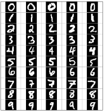
Many real-world data sets are likely to be reducible to a much lower dimension, where each axis represents a non-linear degree of freedom. We do not propose to find these intrinsic degrees of freedom. We only assume their existence in the data set in question. Several definitions of intrinsic dimensionality have been proposed, such as small covering numbers, Assouad dimension, low dimensional manifolds, and Local Covariance Dimension (LCD). In this paper we mostly consider LCD.

Random projection trees (rp-trees) were introduced by [2, 3]. This data structure differs from the kd-tree only in the nature of the splitter used. While the kd-tree always splits parallel to a single axis, the rp-tree splits in essentially a random direction. [2, 3] show that the rp-tree adapts to the intrinsic dimensionality of data (in terms of grouping nearby points in the same cells) much better than the kd-tree. However, NNS (using rp-trees) with the standard kd-tree pruning method still degenerates to brute force search in high dimensions.

The Cover Tree[11] is a new non-space partitioning NNS data structure that exploits the intrinsic dimensionality of data. It achieves very good search time and space usage, but suffers from slow preprocessing [18, 12]. The preprocessing requirements are also very sensitive to noise[11]. For this reason, it is not practical for use on large, high-dimensional and noisy data, such as image databases.

The most popular current high-dimensional NNS technique is Locality-Sensitive Hashing. It is almost practical for the real world, except for its large space usage[36, 8]. The index it builds is often many times larger than the original data, again making it unsuitable for very large databases.

The approximate NNS technique described in [41] proposes two solutions. One is hierarchical k-means trees, which is an example of a Geometric Nearest-Neighbor Access Tree (GNAT) [42]. These trees can suffer from slow preprocessing. The other solution is multiple randomized kd-trees. Since searching through kd-trees in high dimensions degenerates to brute force, [41] obtain approximate seach by simply searching through a fixed number of leaf nodes for each tree. This is similar in spirit to multi-probe LSH, and as we discuss in Section VIII, this approach is very likely to be improved by combining it with our method.

The process described in [1] is also not practical for large, high-dimensional data sets as it requires an eigendcomposition of the gram matrix - an $O(n^{3})$ operation. However, to perform efficient NNS, we will show that the expensive process of manifold learning can be avoided.

Contribution

We propose a data structure (Angle Tree) that for the first time gives us the ability to index large and high-dimensional data sets in practice. Its preprocessing and space requirements are not much greater than a regular kd-tree, while providing fast and highly-accurate NNS capability. It also maintains the simplicity of the original kd-tree.

As we will show, in our implementation using a space partitioning data structure, all we need to extract from the data are the angles that the data region in question makes with the splitting hyperplane (splitter). This angle has meaning even in high-dimensional space by the definition of the dot product.

The Angle Tree is described in Algorithms 1, 2 and 3, and is included in the Appendix. It is conceptually a small modification to any current tree-based indexing technique, such as a kd or rp-tree[2, 3], that adds the power to exploit the intrinsic structure of data during NNS, while introducing a very small probability of error (not finding the true nearest neighbors). While these tree structures can already perform near-neighbor search (ie. only search one cell of the tree), we introduce a new method of efficiently deciding which other cells, if any, also need to be searched. This method is a generalization of the classic kd-tree NNS algorithm for low intrinsic dimensionality data embedded in very high-dimensional space. If there is no intrinsic structure to exploit in a particular data set, then the Angle Tree will behave like a regular kd or rp-tree, with minimal additional overhead.

The remainder of the paper is organized as follows. In Section II we list all definitions used in the paper. In Section III we present the key idea of this paper and prove its correctness. In Section IV we discuss the behaviour of the dihedral angle (between the splitter and the low dimensional manifold region) in high dimensions. In Section V we introduce our method for finding the dihedral angle. In section VI we analyze the accuracy of NNS using Angle Trees. In Section VII we report the results of our experiments. In Section VIII we provide some further comments and suggest directions for future work.

II Definitions

In this section we collect all the definitions used in the paper for the convenience of the reader.

• Ambient Dimension ($D$): is the dimension of the raw data. For example, if data is presented as an $N\times D$ matrix, then the ambient dimension is $D$.

• Intrinsic Dimension ($d$): is the number of degrees of freedom in the data. Again, if data is presented as an $N\times D$ matrix then the intrinsic dimensionality ($d$) is typically much smaller than $D$. The intrinsic dimension is usually not known but can be estimated [15].

• Local Covariance Dimension (LCD): A set S has local covariance dimension $(d,\epsilon,r$) if it has $(1\text{\textminus}\epsilon)$ fraction of its variance concentrated in a $d$-dimensional subspace. More precisely, let $\sigma_{1}^{2},\sigma_{2}^{2},...,\sigma_{D}^{2}$ denote the eigenvalues of the covariance matrix; these are the variances in each of the eigenvector directions. "Set $S\subset\mathbb{R}^{D}$ has local covariance dimension $(d,\epsilon,r$) if its restriction to any ball of radius $\leq r$ has covariance matrix whose largest $d$ eigenvalues satisfy $\sigma_{i}^{2}\geq\frac{1-\epsilon}{d}\left(\sigma_{1}^{2},+\sigma+...+\sigma_{D}^{2}\right)$" [2]

• Intrinsic Plane (IP): is the $d$-dimensional affine subspace associated with the LCD defined above.

• Splitter: the splitting hyperplane of dimension $D-1$ to $\mathbb{R}^{D}$. It splits the data region in question into two not necessarily equal parts.

• Dihedral Angle ($\alpha$): The angle between the splitter and the IP. If the IP has codimension 1, then this angle is simply the angle between their normal vectors (the splitter always has codimension of 1). Otherwise, it is $\pi/2$ minus the angle between the normal vector to the splitter and its projection onto the IP [43].

• Error Angle ($\theta$): This angle reflects the accuracy of the dihedral angle returned by the getAngle() function (see Section V).

• Ambient Distance ($dist(q,p)$): is the distance in the ambient space between points or hyperplanes $q$ and $p$.

• Manifold Distance ($dist_{M}(q,p)$): is the distance between points or hyperplanes $q$ and $p$ when the path is restricted to the data manifold.

• Intrinsic Plane Distance ($dist_{IP}(q,p)$): is the distance between points or hyperplanes $q$ and $p$ when the path is restricted to the IP. If $q$ or $p$ does not lie on the IP, then we project it onto the IP before calculating the distance. Note that $dist_{m}(q,p)\geq dist(q,p)\geq dist_{IP}(q,p)$ if $p$ and $q$ are both points.

• Locality-Sensitive Hashing (LSH): A popular current NNS solution proposed by [28, 10]. In this paper we refer to the random projection implementation of LSH. Its main problem is space usage [36].

• Cover Tree: A relatively new NNS tree structure that is designed to exploit $d$. It does not partition the space, and in fact only requires a metric that satisfies the triangle inequality. Its main problem is preprocessing time[18, 12] and sensitivity to noise [11].

• Random Projection Tree (rp-tree): Data structure introduced by [2, 3]. Similar to kd-tree, but splits in a random direction. Has the property that every $O(dlogd)$ levels, the diameter (distance between two furthest points) of each cell is halved [2, 3].

III Key Idea

(a) kd-tree NNS Search

(b) Manifold Search

Figure 2: kd-tree NNS search ball. Q is query point. G is the nearest neighbor found so far. The top level split is in bold.

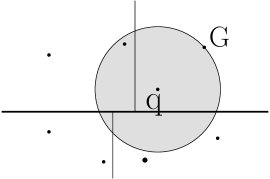
In order to appreciate the key insight of the proposed approach we first explain how a query point $q$ uses the classical kd-tree to carry out the NNS.

A query point $q$ will navigate down a branch of the kd-tree (each pair of branches being split by a splitter) until it reaches the leaf cell in which it is contained. The nearest neighbor in that cell will be identified ($G$ in Figure 2(a)). A search sphere of radius $dist(q,G)$ will be constructed and any neighboring cell which intersects the search sphere will be explored for points which are potentially closer to $q$ than $G$. Effectively this implies that the perpendicular distance between $q$ and the splitter(s), which form the walls of the cell, serve as a lower bound for pruning.

It is well known that in high-dimensional space, the kd-tree NNS degenerates to little better than brute force. We will provide an alternate explanation in Section IV in terms of the distance from $q$ to the walls of its cell.

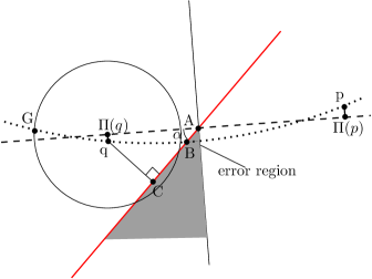
Now if the data lives in a low dimensional manifold, for example, on the dotted line in Figure 2(b) then a better lower bound is the manifold distance $dist_{M}(q,B)$. However, generally the manifold is not known, so we instead approximate $dist_{M}(q,B)$ with the IP distance $dist_{I}P(q,A)$.

In order to calculate the $dist_{I}P(q,A)$ we will use the trigonometric relation

$$dist(q,A)=\frac{dist(q,C)}{\sin\alpha}$$ (1)

The following is the crucial observation which underpins the whole approach.

• In low dimensional space, $\sin\alpha\approx 1$. Thus $dist(q,A)\approx dist(q,C)$ and thus the Angle Tree and kd-tree will behave in a similar fashion.

• In high dimensional space (with low intrinsic dimensionality), $\sin\alpha<<1$, and thus $dist(q,A)$ will be potentially a much tighter lower bound than $dist(q,C).$

• In practice, real data sets rarely follow the equations of a smooth manifold and there will be data points which lie outside the manifold. Also, even if the data forms a smooth manifold, this manifold can be highly curved making it difficult to approximate its local regions with an affine hyperplane. These two factors can cause data points to lie in the error region shown in Figure 2(b). Then the true nearest neighbors could be accidentally pruned.

IV High Dimensional Behavior

We provide a rigorous justification for the behavior of the dihedral angle ($\alpha$) in high dimensional space as noted in Section III. Theorem 1 below is based on Figure 2(b) but generalizes to higher dimensions.

Theorem 1.

Given a random $d$-dimensional hyperplane ($IP$) in $\mathbb{R}^{D}$ and a random affine hyperplane of dimension D-1 (splitter) defined by its normal vector $v\sim N(0,I_{D})$. Let $\alpha$ be the dihedral angle. If $D$ is large, $\sin\alpha$ converges to $\frac{\chi_{d}}{\sqrt{D-\frac{1}{2}}}$, where $\chi_{d}$ is the Chi-distribution with $d$ degrees of freedom [47]. If $d$ is also large,

$$\sin\alpha\sim N\left(\frac{\sqrt{d-\frac{1}{2}}}{\sqrt{D-\frac{1}{2}}},\frac{1}{2D-1}\right)$$

Proof:

As $v$ is a D-dimensional random vector, we can express it as $(x_{1},x_{2},\ldots,x_{D})$ and fix the d-dimensional IP as the hyperplane spanned by the first d axes of $\mathbb{R}^{D}$. Here each $x_{i}\sim N(0,1)$. Based on Figure 2(b), note $\alpha=\pi/2-\angle(v,\Pi v)$ where $\Pi v$ is the projection of $v$ onto $IP$. Thus $\Pi v=(x_{1},x_{2},..,x_{d},0,..,0)$.

$$\sin\alpha=\cos\angle(v,\Pi v)=\frac{v\cdot\Pi v}{|v||\Pi v|}=\frac{\sum_{i=1}^{d}x_{1}^{2}}{\sqrt{\sum_{i=1}^{d}x_{1}^{2}}\sqrt{\sum_{i=1}^{D}x_{1}^{2}}}=\frac{\sqrt{\sum_{i=1}^{d}x_{1}^{2}}}{\sqrt{\sum_{i=1}^{D}x_{1}^{2}}}$$

The numerator and denominator are both chi-distributions with $d$ and $D$ degrees of freedom respectively. For large $D,\,\chi_{D}\sim N(\sqrt{D-\frac{1}{2}},\frac{1}{2})$ [29]. Since we assume $D$ to be very large, the denominator’s variance becomes insignificant relative to its mean, and so we can replace it by its mean.

$$\sin\alpha\sim\frac{\chi_{d}}{\sqrt{D-\frac{1}{2}}}$$

For the case when $d$ is also large, we apply [29] to the numerator as well, yielding

$$\sin\alpha\sim N\left(\frac{\sqrt{d-\frac{1}{2}}}{\sqrt{D-\frac{1}{2}}},\frac{1}{2D-1}\right)$$

∎

V Estimation of the Dihedral Angle

Figure 3: $IP$ indicated by dashed line. Dots represent the data. $m$ is a representative point of the data region. $p$ an arbitrary point on the opposite side of the splitter (red hyperplane) to $m$. We let this region have a LCD with $\epsilon=0$ for clarity.

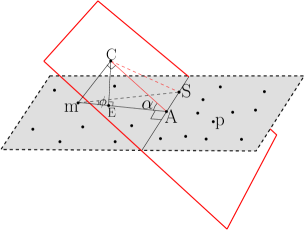
The dihedral angle $\alpha$ between two hyperplanes $P1$ and $P2$ of codimension 1 is related through their unit normals $n1$ and $n2$ by the equation [43]

$$\cos\alpha=n1\cdot n2$$ (2)

Thus if we know the two hyperplanes and their unique normals, calculating the dihedral angle is straightforward. The challenge in our case is that we do not know the equation of the Intrinsic Plane (IP) and furthermore we assume that the IP will change from region to region. In fact, by definition, manifolds are locally like hyperplanes. We could use a PCA-like technique but that would be computationally prohibitive as the complexity of PCA is $O(D^{3})$ where $D$ is the ambient dimension. We will propose a much simpler and more efficient method which is also mathematically rigorous. We refer the reader to Figure 3 for the discussion in this section.

In Figure 3, $m$ is the representative point and $\vec{mC}$ is the normal from $m$ to the splitter. $\alpha=\angle CAm$ is the dihedral angle which can be obtained by projecting $\vec{mC}$ onto the IP. Let $S$ be an arbitary point on the $IP$ (here it is shown to be on the intersection of the two planes but it does not have to be).

An important observation is captured in the following theorem.

Theorem 2.

$\cos\angle CmS=\sin\alpha\cos\phi$ where $\alpha$ is the dihedral angle and $\phi$ is the angle between $mA$ and $mS$ (see Figure 3).

Proof:

Since $\alpha$ is a dihedral angle, $\sin\alpha=\cos(\pi/2-\alpha)=\frac{\vec{mC}\cdot\vec{mA}}{|mC||mA|}$. Also

$$\cos\angle CmS=\frac{\vec{mC}\cdot\vec{mS}}{|mC||mS|}$$

Substituting $\vec{mS}=\vec{mA}+\vec{AS}$ and $|mS|=|mA|/\cos\phi$ in the above equation we get

$$\cos\angle CmS=\cos\phi\frac{\vec{mC}\cdot\vec{mA}+\vec{mC}\cdot\vec{AS}}{|mC||mA|}$$ (3)

Since $\vec{AS}\bot\vec{mA}$, $\vec{AS}\bot\Pi(\vec{mC)}$ where $\Pi(\vec{(}mC))$ is the projection of $\vec{mC}$ onto the $IP$. Clearly also $\vec{AS}\bot\left(\vec{mC}-\Pi(\vec{mC)}\right)$, since that is a vector normal to the $IP$. Then $\vec{AS}$ is normal to the plane spanned by $\Pi(\vec{mC)}$ and $\left(\vec{mC}-\Pi(\vec{mC)}\right)$. Therefore $\vec{AS}\bot\vec{mC}$ and $\vec{mC}\cdot\vec{AS}=0$
Then equation 3 becomes

$$\cos\angle CmS=\cos\phi\frac{\vec{mC}\cdot\vec{mA}}{|mC||mA|}=\cos\phi\sin\alpha$$

∎

We should note that the proof of this theorem does not make use of $S$ lying on the intersection between the $IP$ and the splitter, and so this angular relation is true for any $\vec{mS}$ on the $IP$.

Corollary 1.

$\forall\vec{v}\parallel IP\,\,\,\,\angle(\vec{v},\vec{mC})\leq\pi/2-\alpha$

Proof:

When $\pi/2\geq\phi\geq 0$, $\cos\angle CmS\leq\sin\alpha=\cos(\pi/2-\alpha)$. As $\phi\rightarrow 0$, $\cos\angle CmS\rightarrow\cos(\pi/2-\alpha)$ and hence $\angle CmS\rightarrow\pi/2-\alpha$ from below. ∎

Corollary 2.

The dihedral angle $\alpha\geq\angle mSC$

Proof:

Since $\angle CmS\geq\pi/2-\alpha$, $\alpha\geq\pi/2-\angle CmS=\angle mSC$ ∎

Theorem 2 and the corollaries suggest the following algorithm for estimating alpha:

We take the center of the data region and sample a constant number ($k)$ of random data points within the region. We then subtract the center from all of these points to obtain $k$ random vectors that will represent the region (there are many other methods for obtaining these $k$ random vectors). We calculate the angle that all of these vectors make with the normal to the splitter $\vec{mC}$ (each region has one splitter). The smallest of these $k$ angles will be within a small range of $\pi/2-\alpha$ ($\angle CmA$ in Figure 3), the true angle between $\vec{mC}$ and the $IP$ (See the Appendix for pseudocode of this procedure). In order for this to work, at least one of the random vectors must be within a small angle of $\vec{mA}$ (as close to parallel as possible). The probability of this occurring depends on the dimensionality of $IP$, as we will show.

V-A Evaluation of Random Vector Strategy

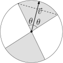
In order to evaluate this strategy, we form the following problem. We assume the data is evenly distributed within a d-ball of unit radius, centered at the origin, and we have some fixed vector $\vec{v}$ within this space. We then generate $k$ random vectors within the ball, and calculate the probability that not one of these is within some small angle $\theta$ (error angle) of $\vec{v}$ (please refer to Figure 4 for illustration). We denote the volume of the d-ball segment spanning the vectors that are close to $\vec{v}$ by $s$, and the volume of the entire d-ball by $S$. Since we assumed the data to be evenly distributed, every random vector has a constant probability $s/S$ of landing within the aforementioned segment. $s$ has volume given by the formula for the d-dimensional cone $Base\times Height/d$ [44] plus the volume of the hypersphere cap given by the formula described in [45]. Combining these two formulas, the ratio $s/S$ has the value given by:

$$s/S=2\left(\frac{1}{2}-\cos\theta\frac{\Gamma[1+\frac{d}{2}]}{\sqrt{\pi}\Gamma[\frac{d+1}{2}]}{}_{2}F_{1}\left(\tfrac{1}{2},\tfrac{1-d}{2};\tfrac{3}{2};\cos^{2}\theta\right)\right)+\frac{2\cos\theta\sin^{d-1}\theta\cdot\Gamma[1+\frac{d}{2}]}{d{\sqrt{\pi}\cdot\Gamma[1+\frac{d-1}{2}]}}$$ (4)

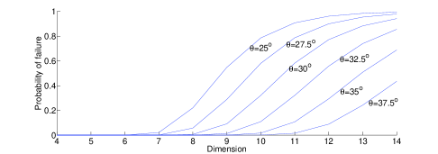
where $\Gamma$ is the Gamma function and ${}_{2}F_{1}$ is Gauss’ hypergeometric function [46]. Note that this ratio depends only on $\theta$ and the intrinsic dimension $d$. Monte Carlo experiments confirm the values given by this formula.

Figure 4: $\theta$ determines the width of the target region (shaded). If a random vector makes an angle close to $180^{o}$ to $\vec{v}$, we simply multiply it by -1 in order to obtain a vector close to $\vec{v}$. Hence our target region’s volume is doubled. The dashed line divides the target region into two parts; a hypercone and a hypersphere cap.

The probability that all $k$ vectors miss the segment is then $(1-s/S)^{k}$. We show that this probability can be made very small for $k\thickapprox 2,000$, $\theta\thickapprox 30^{o}$ while $d\leq 10.$ Beyond that dimension, to maintain a small $\theta$, $k$ would have to grow exponentially. So in Section V, as long as $d$ is not too large, we can get a vector $\vec{mS}$ that is within $\theta$ of $\vec{mC}$.

Figure 5: Probability of all the 2000 random vectors missing a segment (failure) of width $\theta$ within a d-dimensional ball is sensitive to both $\theta$ and $d$. The formula used to build this graph is $(1-s/S)^{2000}$ where s/S is given by Equation 4.

One obvious problem with this approach is that if the data is noisy, then the vectors we generate do not lie exactly on the $IP$. This causes some inaccuracy in determining $\alpha$. Our approach for dealing with this involves simply ignoring a constant portion of the most extreme angles, attributing them to noise. This is described further in Section VII.

Another problem occurs when the region in question is large, where the manifold curves sharply with respect to the splitter. In this case there is no low dimensional $IP$ that approximates the data well.

Figure 6: One of the random vectors needs to be (close to) normal to the splitter for the Angle Tree to behave like a regular kd-tree. Here the manifold despite being 1-dimensional, bends sharply w.r.t. the splitter, and so there are many such vectors. When the region is made smaller by further splits, the manifold will become flatter, and so the directions of the vectors generated in the region will be more limited.

The case in Figure 6 is not a pathological one. Despite the data having intrinsic dimension of 1, the region in question is too large to be approximated by a 1-dimensional $IP$. For this reason, we consider this data region to be 2-dimensional for our purposes.

In order for this technique to not prune any regions incorrectly, we must find that $\alpha=\pi/2$ here - we use the regular kd-tree search lower bound, since $dist(q,A)=dist(q,C)/\sin\alpha=dist(q,C)$ in this case. In order for this to happen, at least one of the randomly generated vectors must make an angle of $\pi/2$ (or close to it) with the splitter.

Then, we do not gain or lose anything compared to the standard kd-tree pruning method, in this case. As we continue to split the data, the regions will become small enough that they can be approximated by a low dimensional $IP$.

Another possibility: if the data lies on a d-dimensional manifold, but we consider a region where the manifold curves sharply, but only in one other dimension. In this case, the region can still be approximated by a d+1 dimensional $IP$. For example, the data in Figure 6 could have a very large ambient dimension, but this region can still be approximated by a 2-dimensional $IP$. Our method will be robust to this possibility, since from Theorem 1, the angle between the d+1 dimensional $IP$ and the D-1 dimensional splitter is still very likely to be much smaller than $\pi/2$, giving the angle tree a large performance boost over the standard kd-tree pruning.

V-B Effect of Error Angle on Pruning Calculation

We refer again to Figure 3. Let $\vec{mS}$ be an extension of the randomly generated vector making the smallest angle with $\vec{mC}$. Then if we have some estimation of $d$, and by referring to Figure 5, we can say that with high probability $\vec{mS}$ is within $\theta$ (of some appropriate size) of $\vec{mC}$ – $\phi<\theta$. Then making use of Theorem 2 again, $\cos\angle CmS=\sin\alpha\cos\phi>\sin\alpha\cos\theta$, and from this we can derive

$$|mA|>\cos\theta|mC|/\sin\angle CSm$$

where $\angle CSm$ is our slightly erroneous estimate for $\alpha$ and $\cos\theta$ is compensation for this error.

Putting the query point $q$ in the place of $m$, we now have a ’safe’ lower bound on $dist(q,A)$, and it tightens as $\theta$ is made smaller (by generating more random vectors, for instance). This bound should still be much tighter than $dist(q,C)$.

VI Error Region

Figure 7: Illustration of LCD. If $\epsilon$ is small, then the distance of data point $p$ from $IP$ is a relatively small component (on average over all $p$) of the distance of $p$ from the mean of the data region.

Figure 8: A is the geometric mean of the data. Error Region is blue. Red line is splitter. Vertical black line through A is perpendicular (ideal) splitter. The hypercylinder is made up of the $IP$ (a d-ball with radius $a$ - represented by the horizontal dashed line) and an infinite number of (D-d)-balls centered on each point in the $IP$ (not data point) and perpendicular to the $IP$. In the case when $d=1$ and $D=2$, the hypercylinder is a rectangle as shown. Data is evenly distributed within the hypercylinder.

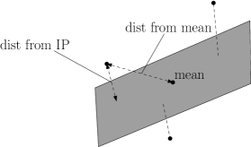
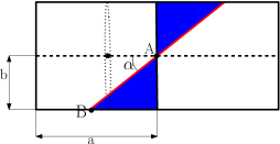
In Figure 2(b) we noted an error region, where any point $p$ falling into it has the property $dist_{IP}(q,p)<dist(q,A)$ and hence breaks one of our assumptions. The cell containing this point might be pruned using our algorithm, even though it contains a neighbor that is nearer to $q$ than the best-so-far found neighbor. In order to analyze this possibility we need a model of the region in question. For this, we make use of the property of LCD as described in [5]; if the data has covariance dimension $(d,\epsilon,r)$ for some $r$, then any data region that fits entirely inside a ball of radius $r$ will have

$$(avg\,dist^{2}\,from\,IP)\leq\epsilon\cdot(avg\,dist^{2}from\,mean)$$

where the $avg\,dist$ and $mean$ (geometric mean on all the dimensions) are taken across all the data points in the region (see Figure 7).

We assume that $\epsilon$ is small ($0\leq\epsilon\leq 0.1$). If we let the noise be uniform, we have the following model: points are uniformly distributed within the hypercylinder shown in Figure 8. The $IP$ itself is a $d$-ball with radius $a$. Centered on each point on the $IP$ we have a $(D-d)$-ball normal to $IP$ with radius $b$. $a$ and $b$ are chosen so that the data being distributed uniformly within the hypercylinder, has $avg\,distance{}^{2}$ within $IP$ equal to 1, and the $avg\,distance{}^{2}$ from subspace equal to $\epsilon$. The $avg\,distance{}^{2}$ from mean is then equal to $1+\epsilon$, so the model satisfies the above constraint (since $\epsilon\leq\epsilon+\epsilon^{2}$) while being close to the maximal noise case (since $\epsilon^{2}$ is insignificant for small $\epsilon$). Then the ratio of the volume of the error region $v$ to the volume of the entire region $V$ described by the model corresponds to the proportion of points that fall within the error region.

We obtain it by integrating the Error Region volume along $z$ (any axis within $IP$) from $B~{}(z=-b/\tan\alpha)$ til $A~{}(z=0)$ and multiplying by 2. We denote the volume of a $k$-ball with radius $l$ by $B^{k}(l)$ and the volume of a hypersphere cap of height $m$ and dimension $k$ by $C_{l}^{k}(m)$. By considering the intersection of the $IP$ (which we assumed to be a d-ball) and a 2-dimensional plane through $A$, and noting that this intersection must be a circle, we see that the radius of the (d-1)-ball in the $IP$ subtended by the integration slice $z$ units away from $A$ will have radius $\sqrt{a^{2}-z^{2}}$. The volume subtended from the (D-d)-ball in the noisy directions will equal $C_{b}^{D-d}\left(b+ztan\alpha\right)$. Hence the total volume of the Error Region is given by:

$$\frac{v}{V}=\frac{2\int_{-b/\tan\alpha}^{0}\,B^{d-1}\left(\sqrt{a^{2}-z^{2}}\right)\times C_{b}^{D-d}\left(b+ztan\alpha\right)dz}{B^{d}(a)\times B^{D-d}(b)}$$ (5)

Where $D$ is the ambient dimension, $d$ is the intrinsic dimension of $IP$, $a=\sqrt{3/d}$, $b=\sqrt{3\epsilon/(D-d)}$, and $\epsilon$ is the LCD coefficient. We often find that this ratio is very small when $d\ll D$ and $\epsilon\leq 0.1.$

Proposition 1.

When $a=\sqrt{3/d}$ and $b=\sqrt{3\epsilon/(D-d)}$, then the data distributed uniformly within the hypercylinder, has $avg\,distance{}^{2}$ within $IP$ equal to 1, and the $avg\,distance{}^{2}$ from subspace equal to $\epsilon$.

Proof:

We assumed that the first d axes are: $x_{i}\sim[-a,a]$. Then

$$E\left(\sum_{i=1}^{d}x_{i}^{2}\right)=\sum_{i=1}^{d}E\left(x_{i}^{2}\right)=d\cdot E\left(x_{1}^{2}\right)=1\Rightarrow E\left(x_{1}^{2}\right)=\frac{1}{d}$$

because of the linearity of expectation, and all the $E(x_{i}^{2})$’s are equal.

$E\left(x_{i}^{2}\right)=\frac{\int_{-a}^{a}\,x^{2}}{2a}=\frac{\frac{1}{3}\times 2a^{2}}{2a}=\frac{a^{2}}{3}=\frac{1}{d}$

giving $a=\sqrt{3/d}$

By a similar process we get $b=\sqrt{\frac{3\epsilon}{D-d}}$

∎

It can be seen that the Error Region is smaller if $\alpha$ is made larger (our splitter is closer to the ideal splitter). In Section VIII we give one possible way to achieve this.

VII Experiments and Analysis

VII-A Design of Experiments

In this section the Angle Tree is experimentally compared against the cover tree and locality sensitive hashing (LSH). They are the two most popular and most recent developments in high-dimensional NNS. The Angle Tree is also compared against Partial Brute Force (PBF). If for an experiment the Angle Tree achieved an average accuracy of 90% or 0.9 when searching for k-nearest neighbors (meaning that all k neighbors returned were the true nearest neighbors 90% of the time, as as verified by a full brute force search), then PBF, searching randomly through unindexed data, must search through $\%(100\times 0.9^{1/k})$ to achieve the same average accuracy.

The comparison will be based on preprocessing time, space complexity, query time and accuracy. The comparison vis-a-vis kd-trees and rp-trees is not reported as the NNS query using the latter two data structures degenerates to a brute force search in high dimensions if the standard pruning bound is used.

It it worth recalling that the original rp-tree (as proposed by the authors) can only be used to efficiently answer near neighbor search (where we only search through a single cell and terminate - see Section III for details of why this often misses the true nearest neighbors). If the kd-tree search strategy is used with the rp-tree, then the search degenerates to brute force. In fact, the principal aim of Angle Trees is to extend rp-trees (and kd-trees) to make NNS in high dimensions efficient and accurate.

VII-A1 Implementation Details

The Angle Tree was implemented on top of the rp-tree code base available from the authors website [2]. We did not use the error angle adjustment in our implementation, since speed seemed to be more of a bottleneck than accuracy. All experiments were performed on an AMD dual core 1 GHz processor with 4GB of RAM. In our experiments we will refer to the Angle Tree as angle rp-tree to emphasize its connection with random projections and rp-trees.

Cover tree code was obtained from the authors website [11]. This code was used to attempt to preprocess all of the data sets used. The cover tree performance data is taken from [12].

LSH (where the hash functions are a series of random projections) performance was inferred from the performance of near neighbor search in a single rp-tree. If $t$ independent rp-trees are built, then each one has a similar probability $p$ of having both the query point $q$ and its nearest neighbor hashed to the same cell. Then the probability of not finding the nearest neighbor in any of the $t$ trees is $(1-p)^{t}$. The average search time is then $xt$, where $x$ is the average search time for a single rp-tree near neighbor search. The probability $p$ obviously depends on the size of the cells - or the number of LSH hash buckets. This data is presented in Table III.

VII-A2 Data Sets

Several well known real data sets were used for comparison. We also generated two synthetic data sets on high-dimensional spheres. The details are listed in Table II in the Appendix. It is worth emphasizing that we used extremely high-dimensional, real world data sets (e.g., Reuters Bag of Words, Mnist and Yale Face image database) which are extremely noisy and hard to index. For overview of all the data sets used, see Appendix.

VII-A3 Comparison Metric

The fundamental metric used to compare the data structures is number of distance calculations (NDC) - which is defined as the number of times euclidean distance between two points is calculated. This metric is hardware independent.

NDC is used as a proxy to measure the running time of the algorithm, being by far the most computationally intensive part of the algorithm. NDC correlates very strongly with the actual running time of the algorithm, and was used in [12] to evaluate the cover tree.

VII-A4 Parameters

There is one important parameter in angle rp-trees whose effect needs to be measured, namely, the Ignore Outlier (IOut) parameter.

IOut controls the effect of noise in the data during the estimation of the dihedral angle. IOut is the proportion of the angles between the random vector and the normal to the splitter ($\vec{mC}$ in Figure 3) that will be ignored. The assumption is that very small angles are caused due to the presence of outliers, since outliers do not lie on the $IP$ and do not conform to Theorem 2.

For example, suppose one thousand random data vectors are generated and for each such vector, the angle with the normal to the splitter is calculated. These angles are then sorted in an increasing order and if the IOut value is 0.1, then the $100^{th}$ angle is the estimated value of the dihedral angle.

IOut controls the trade-off between accuracy and search time. High values of IOut will inflate the estimation of $dist_{IP}(q,A)$. This will result in more aggressive pruning but could result in some nearest neighbors being missed.

Another parameter that we vary is the number of levels in the tree. This is significant for the LSH analysis as it determines the number of hash buckets. More and smaller buckets usually translates to lower accuracy but faster search time.

The other LSH parameter is $t$, the number of trees (hash functions) over which we infer the performance of LSH.

VII-A5 Experiments

The following three experiments were conducted. In E1, we measure preprocessing efficiency, and in E2 and E3 we measure search efficiency.

• For each data set, the angle rp-tree was constructed and the NDC was recorded. We note that NDC has the same complexity as angle computations and projection onto splitter (O(D), since they all involve a dot product) and so for the angle rp-tree we include them in the NDC value. We also used the cover tree code to see whether preprocessing the various data sets would cause a crash. We used the standard rp-tree (with various number of levels) as an implementation for LSH.

• For each data set, one thousand random data points were chosen and used to simulate queries. In this way the query points were guaranteed to also come from the data manifold. The angle rp-tree was then used to search for 1-NN with various IOut parameter values for each query point. The NDC was recorded during the search process and then averaged over the one thousand queries.

• For the Mnist and KDD data, a search for 2-NN was also carried out as comparative data was available from [12].

Figure 9: Here is the main advantage of the angle rp-tree over the cover tree; cover tree preprocessing time - the number of distance computations in the construction of the data structure - is exponential in $d$. [11]

Figure 10: Speedup over partial brute force. The amount of data that the brute force randomly searches through in order to get the same average accuracy as our method. To get $x\%$ accuracy, partial brute force must on average search through $x\%$ of data for 1-NNS and $10\sqrt{x}\%$ of data for 2-NNS. ’in10’ means that the IOut value for an experiment was 0.1 – we ignored 10% of the most extreme angle values.

Figure 11: Search performance of angle rp-tree vs cover tree for 1-NNS. Various IOut values are used to balance speed and accuracy. While cover tree is capable of 100% accuracy, our method can come very close with comparable running time.

Figure 12: Search performance of angle rp-tree vs cover tree for 2-NNS. Various IOut values are used to balance speed and accuracy. While cover tree is capable of 100% accuracy, our method can come very close with comparable running time.

VII-B Results and Analysis

We now report on the results of the three different experiments under varying conditions.

VII-B1 E1

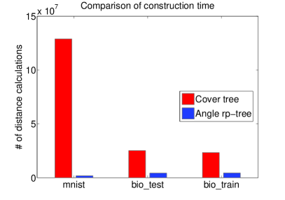
Cover Tree

See Figure 9. Theoretically the preprocessing time of angle rp-trees is nearly of the order of a standard kd-tree or rp-tree, which is $O(nlogn)$. The only additional overhead is the calculation and storage of the dihedral angle for each data region. Since the number of data regions (nodes) is $O(n)$, and we calculate a constant number of angles ($k$) in each data region, the complexity of angle rp-tree is $O(nlogn+nk)$ which is $O(nlogn)$.

For cover trees, the theoretical preprocessing time is:
$O(c^{6}n\log n)$ where $c$ (the KR-dimension) $\sim 2^{d}$ and potentially much larger for noisy data. A single noisy point can make $c$ grow arbitrarily [31].

The preprocessing in our experiments for the cover tree and angle rp-tree are shown in Figure 9. It is clear that the preprocessing time of the angle rp-tree is a small fraction (less than 1%) of the cover tree.

Another factor that is not reflected in the results is that even though the cover tree space requirements are O(n) just like the kd-tree, the data points appear multiple times in the structure. Thus cover tree’s space complexity has a higher constant. Its memory usage is often three to five times greater than the size of the data set [12].

We have only shown results on three data sets for which the comparison data was available. The cover tree crashed during construction for the Reuters Bag of Words and the synthetic sphere databases. It crashed likely due to overflow of the recursion stack during construction [18] due to those data sets having an intrinsic dimension that is too large.

LSH

See Table III. The preprocessing time of LSH is similar to rp-trees except that there are $t$ trees (hash functions) and so roughly $t$ times as much preprocessing (the constant number of angle calculations that are not required in LSH become relatively trivial anyway, when the data set is large). However, LSH preprocessing time has no dependence on $d$ and is unaffected by noise, and so is fairly efficient.

Due to there being $t$ trees and each data point is hashed into each tree, LSH space complexity is significantly greater than the angle rp-tree. It is difficult to say how much more exactly since only the hash values of the data are stored, but [36, 8] reports it to be significant - several times the size of the original data. As we will see later, when $t$ is reduced, then accuracy and/or search speed suffers. For larger data sets than the ones tested here, [36, 8] note that LSH often requires $t$ to be of the order of 100 to obtain acceptable search speed and accuracy.

VII-B2 E2

PBF

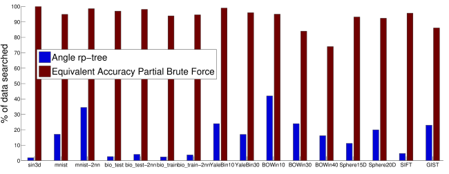
See Figure 10. Here we see the speedup of angle rp-tree over PBF. Even in 30,000+ dimensional data like the images database, we find the true nearest neighbors 95%+ of the time while searching <20% of the data. This indicates very strongly that the curse of dimensionality can be managed when data has a low intrinsic dimensionality, without any dependence on the ambient dimension. We believe that if the database had more items (Yale Face has <2500 items) the angle rp-tree indexing would give an even greater speedup, similar to the KDD data sets.

The noisiest (or least structured) and hence most difficult data set was the Reuters Bag of Words data set. For this data set we had to search through 42% of the data in order to achieve 95% accuracy for 1-NNS. We could also search through 24% of data to achieve 85% accuracy. This second result seems to be more practical to us, though the user would have to accept a 15% error rate. Additionally, in the 15% of cases where an incorrect neighbor was returned, it was usually a small error. As far as we know, no one else had indexed this kind of data set with any significant success.

The sin3D, as well as the 15D and 20D Sphere synthetic data sets are included to indicate what sort of complexity of structure the real world data sets must have, if they have similar performance to the synthetic data sets whose structure is known. The 15D Sphere data set gave much better results, and was close in performance to the KDD bio data sets, whereas the 20D sphere data set was closer to the Reuters Bag of Words data set. This is consistent with our analysis in Section V, which suggested that the intrinsic dimensionality must be not much greater than ten in order for the dihedral angle to be accurately estimated.

Results for the sin3D data set were 100% accurate, with most of the angles being over $80^{o}$. The angle rp-tree reduced to the kd-tree for this low-dimensional data set.

Cover Tree

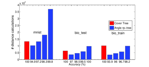
See Figure 11. The angle rp-tree achieves accuracy well over 95% with search speed similar to or faster than the cover tree, although the cover tree achieves 100% accuracy.

The angle rp-tree seems to slow down significantly as we try to approach 100% accuracy with noisy data. We search through twice as much data for the mnist data set in order to increase accuracy from 98.3% to 99.8%. This is likely because the $IP$ starts to include more and more rare, noisy directions as we reduce the IOut parameter value. As the $IP$ grows in dimension, the dihedral angle grows quite rapidly causing the pruning multiplier $1/\sin\alpha$ to shrink. This causes the algorithm to prune a lot less cells for very little gain in accuracy (when the noisy points turn out to be the true nearest neighbors). Due to this we can only really achieve 100% accuracy as well as fast running time when the data is not noisy, and hence can be well estimated by a low dimensional $IP$. For noisy real world data, we must at this stage settle for 95+% accuracy.

LSH

See Table III. In this table $t$ and $p$ are chosen so that the accuracy corresponds to one of the results in Figure 10.

We can see that for the Reuters Bag of Words and mnist data sets, LSH with large $t$ parameter is often several times faster on average than the angle rp- tree, while having a similar accuracy. However, when we reduce $t$ (in order to alleviate the space usage) but wish to maintain accuracy, a tree with less levels must be built. Then, since the leaf cells will contain more data, the probability that the leaf cell into which the query point is hashed will contain its true nearest neighbor, is made higher. This in turn makes LSH slower. In fact, it can be seen that when $t$ is made too small, LSH becomes significantly slower and less accurate than the angle rp-tree.

It is also worth noting that in Table III, when considering the Yale Face image database, LSH is significantly slower and less accurate (as well as more space consuming) than the angle rp-tree. We believe this is because the Yale Face image database is less noisy than mnist and Reuters BOW, and can be better approximated by a low dimensional $IP$.

VII-B3 E3

PBF

See Figure 10 - those columns labeled 2nn. The angle rp-tree searches through approximately twice as much data on average for 2-NNS than 1-NNS. This is logical since the second nearest neighbor is further away from the query point, making the search sphere (see Section III) larger, causing the algorithm to prune less subtrees. In this way the angle rp-tree behaves as it should. The kd-tree operating in the intrinsic space of the data would likely perform in a similar way.

Cover Tree

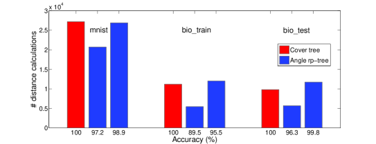
See Figure 12. These results are roughly the same as in E2. The angle rp-tree introduces a small probability of error while achieving comparable search speed to the cover tree.

VIII Discussion

Multi-probe Locality Sensitive Hashing

This is a variation of LSH, where instead of only checking one bucket, multiple buckets are probed. In some implementations, the buckets are sorted by probability that they contain the true nearest neighbor, and only the top few are checked. The purpose of this is to reduce the space requirement of LSH by reducing the number of hash functions that are needed to maintain high accuracy.

The problem with this approach is that a constant number of buckets will be checked with each query, whereas with the angle rp-tree it is often the case that the entire tree may be pruned after checking one or two cells. There is no set number of buckets to check.

Additionally, current implementations of multi-probe LSH are based on calculating the distance of the query point to the splitter [36]. However, as we saw in Theorem 1, since random splitters make significantly varying angles with the data, this distance alone is not the best way of ranking the cells. The angle rp-ree seems to be a promising way to improve current multi-probe LSH implementations.

We have shown that even at this early stage, our algorithm can compete with the state of the art algorithms in terms of running time and accuracy, while being significantly superior in terms of space and preprocessing requirements. Additionally, it is likely to be much simpler to use and implement, since it is not a major modification to the well known kd-tree. We have also provided some new insight on the nature of the curse of dimensionality in the context of NNS.

Future Work

A simple improvement to the random splitter (as used in the rp-tree) would be a splitter whose normal vector lies on or very close to the $IP$, but is still random within this restricted space. This can be achieved by generating some constant number of random vectors in the data as before, and then averaging them, finding their median, or combining them in some arbitrary way. A splitter generated thus would make a much larger angle with $IP$ than a random splitter, and make the error region discussed earlier much smaller.

It seems very likely to us that there is a superior and more robust method for estimating the dihedral angle with noisy data, such as a Kalman filter type of process.

The way we deal with noise in the data, and the effect it has on the dihedral angle estimation, is quite simplistic. It is almost certain that there are more robust ways for doing this.

The exact relationship between the error angle compensation (multiplying by $\cos\theta$) and the search speed hasn’t been analyzed yet. In fact, no guarantees on search speed, even in the average case, have been established.

Data set	Size	D	d	Description
sin3D	10,000	3	3	rp-tree example data
mnist [32]	60,000	784	5-10	Handwriting
bio_train [33]	145,751	75	6	KDD
bio_test [33]	139,658	74	6	KDD
Extended Yale Face B Cropped [34, 35]	2432	32,256	8	Human faces. Various people. Varying lighting
Reuters Bag of Words (BOW) [39]	11,887	6100	10-40	News articles word counts
15D Sphere	100,000	15	14	Synthetic
20D Sphere	100,000	20	19	Synthetic
SIFT[40]	1,000,000	128	15-30	Image descriptors

TABLE II: Overview of the data sets. D is the dimensionality of the data set and d is the approximate intrinsic dimension.

Levels in tree	Avg. Per Search	Accuracy (%)	Number of Trees	Projected Accuracy (%)	Avg. Per Search over all hashes	Avg. Per Search	Accuracy (%)
LSH with RP-tree						Angle rp-tree
mnist
12	205.8	21	13	95.4	2675.4	10272.0	94.9
10	269.1	21.2	13	95.5	3498.3	”	”
8	613.8	27.4	10	96	6138	”	”
4	5855.3	51.7	4	94.6	23,421.2	”	”
3	9144.8	61.1	3	94.1	27,434.4	”	”
bio_train
14	195.9	28.3	9	95	1763.1	3561.8	93.9
bio_test
14	183	29.6	10	97.1	1830	3635.8	97
Extended Yale Face B Cropped
9	169.2	57.4	5	98.6	846	620.5	99
Reuters Bag of Words
12	217.9	33.3	5	86.8	1089.5	2917.8	84
15D Sphere
17	192.3	13.2	19	93.2	3653.7	11,507	93.2
20D Sphere
17	204.3	10.6	26	94.6	5311.8	20,757	94.2

TABLE III: Number of distance function calls for near neighbor search (only checking one cell in the tree) for the mnist database. 1-NSS. This table compares the angle rp-tree with LSH, where the hashing function is a series of random projections.

procedure $createAngleTree(listofpointspointList,~{}treetype)$

1:  tree_node node {Create node}

2:  if $size(pointList)\leq minSize$ then

3:     $node.data\leftarrow pointsList$ {This will be a leaf node}

4:  else

5:     $node.splitter\leftarrow genSplitter(treetype,pointList)$ {Generate splitter based on the treetype. This splitter will have a direction (its normal vector) and a threshold}

6:     $node.angle\leftarrow getAngle(node.splitter,pointList)$ {Our only modification to regular tree creation}

7:     $node.negChild\leftarrow createAngleTree(p\in pointList:~{}p\cdot node.normal\leq threshold,~{}treetype)$

8:     $node.negChild\leftarrow angleTree(p\in pointList:~{}p\cdot node.normal>threshold,~{}treetype)$

9:  end if

procedure $getAngle(splitter,~{}pointList)$

1:  $angles\leftarrow[~{}]$

2:  $center\leftarrow$median (or mean) of pointList for each axis

3:  $ret\leftarrow 0$

4:  for $i=1$ to k do {k is some not very large constant, say 2000}

5:     $p\leftarrow$ random point from pointList

6:     $v\leftarrow(p-center)$ {v is random vector within region containing pointList}

7:     $angles.append(\arccos\left(\frac{abs(<v,\,splitter.normal>)}{|v||splitter.normal|}\right)$ {angle between v and splitter.normal}

8:  end for

9:  angles.sort()

10:  return  $angles[k(1-IOut)]$ {IOut is the Ignore Outlier parameter}

Pruning procedure during NNS

1:  $q\leftarrow query~{}point$

2:  $closestSoFar\leftarrow dist(q,~{}closest~{}neighbor~{}found~{}so~{}far)$

3:  We now modify our pruning criterion during NNS from:

4:  if $dist(q,~{}node.splitter)\geq closestSoFar$ then

5:     prune node’s other child (where $q$ did not come from)

6:  end if

7:  to:

8:  if $dist(q,~{}node.splitter)\cos\theta/\sin(node.angle)\geq closestSoFar$ then

9:     prune node’s other child (where $q$ did not come from) {$\theta$ is a small, constant Error Angle determined by k and d (see Section V)}.

10:  end if

———————

References

- [1] A global geometric framework for nonlinear dimensionality reduction. J. B. Tenenbaum, V. De Silva and J. C. Langford (2000). Science 290 (5500), 2319-2323.
- [2] Freund, Yoav; Dasgupta, Sanjoy Random projection trees and low dimensional manifolds. In Proceedings of the 40th annual ACM symposium on Theory of computing, Pages 537-546, 2008.
- [3] Freund, Yoav; Dasgupta, Sanjoy; Kabra, Mayank; Verma, Nakul Learning the structure of manifolds using random projections NIPS, 2007
- [4] Ting Liu, Andrew W. Moore, Alexander Gray and Ke Yang An Investigation of Practical Approximate Nearest Neighbor Algorithms NIPS, 2004
- [5] Freund, Yoav; Dasgupta, Sanjoy Random projection trees and low dimensional manifolds Lecture, University of California, San Diego, http://www.stanford.edu/group/mmds/slides2008/dasgupta.pdf accessed on 15/10/2009, 2008
- [6] Songrit Maneewongvatana and David M. Mount It’s okay to be skinny, if your friends are fat Center for Geometric Computing 4th Annual Workshop on Computational Geometry, December 1999
- [7] Jose A. Costa and Alfred O. Hero III Manifold Learning Using Euclidean K-Nearest Neighbor Graphs Acoustics, Speech, and Signal Processing. Proceedings. (ICASSP ’04). IEEE International Conference, May 2004
- [8] Alexis Joly and Olivier Buisson A Posteriori Multi-Probe Locality Sensitive Hashing International Multimedia Conference, Proceeding of the 16th ACM international conference on Multimedia, 2008
- [9] Alexandr Andoni; Piotr Indyk Near-Optimal Hashing Algorithms for Approximate Nearest Neighbor in High Dimensions Communications of the ACM, SPECIAL ISSUE: Breakthrough research: a preview of things to come, 2008
- [10] Alexandr Andoni Nearest Neighbor Search: the Old, the New, and the Impossible PhD thesis, Massachusetts Institute of Technology 2009, September 2009
- [11] Alina Beygelzimer; Sham Kakade; John Langford Cover Trees for Nearest Neighbor ACM International Conference Proceeding Series; Vol. 148, Proceedings of the 23rd international conference on Machine learning, 2006
- [12] Comparison of the Cover Tree and sb(S) Datastructures Additional Experiments http://hunch.net/~jl/projects/cover_tree/paper/ addendum/comparison.ps, January 2005
- [13] Piotr Indyk Near-Optimal Hashing Algorithms for Approximate Near(est) Neighbor Problem Lecture, Massachusetts Institute of Technology, http://www.mit.edu/~andoni/papers/cSquared.pdf accessed on 12/10/2009
- [14] Piotr Indyk HIGH-DIMENSIONAL COMPUTATIONAL GEOMETRY PhD thesis, Stanford University, September 2000
- [15] Peter J. Verveer, Robert P.W. Duin "An Evaluation of Intrinsic Dimensionality Estimators" IEEE Transactions on Pattern Analysis and Machine Intelligence, vol. 17, no. 1, pp. 81-86, Jan. 1995, doi:10.1109/34.368147
- [16] D. T. Lee1 and C. K. Wong (1977) Worst-Case Analysis for Region and Partial Region Searches in Multidimensional Binary Search Trees and Balanced Quad Trees Acta Informatica, Volume 9, Pages 23-29, 1977
- [17] Marius Muja, David G. Lowe Fast Approximate Nearest Neighbors with Automatic Algorithm Configuration VISSAPP (1) 2009: 331-340
- [18] Javen Qinfeng Shi Introduction to Cover Tree Lecture, SML of NICTA RSISE of ANU October, http://users.rsise.anu.edu.au/~qshi/talk/introduction%20to%20covertree060815.pdf accessed on 10/11/2009, 2006
- [19] Peter N. Yianilos Locally lifting the curse of dimensionality for nearest neighbor search Symposium on Discrete Algorithms, Proceedings of the eleventh annual ACM-SIAM symposium on Discrete algorithms, 2000
- [20] Yury Lifshits Nearest Neighbors in Doubling Metrics Algorithmic Problems Around the Web #7 Lecture, CalTech, CS101.2, http://yury.name/algoweb/07algoweb.pdf accessed on 12/10/2009, Fall’07
- [21] Donghui Yan; Ling Huang; Michael I. Jordan Fast Approximate Spectral Clustering International Conference on Knowledge Discovery and Data Mining, Proceedings of the 15th ACM SIGKDD international conference on Knowledge discovery and data mining, 2009
- [22] Roger Weber; Hans-Jorg Schek; Stephen Blott A Quantitative Analysis and Performance Study for Similarity-Search Methods in High-Dimensional Spaces Very Large Data Bases, Proceedings of the 24rd International Conference on Very Large Data Bases, 1998
- [23] R. Berinde and P. Indyk Sparse recovery using sparse random matrices MIT-CSAIL Technical Report, 2008
- [24] S. Dasgupta and A. Gupta An elementary proof of the Johnson–Lindenstrauss lemma Technical report 99–006, U. C. Berkeley, March 1999
- [25] Chinmay Hegde; Richard G. Baraniuk; Michael B. Wakin Random Projections for Manifold Learning NIPS, December 2007
- [26] Yoav Freund, Sanjoy Dasgupta, Mayank Kabra, Nakul Verma Learning the structure of manifolds using random projections NIPS, 2007
- [27] Dasgupta, S. Freund, Y Random projection trees for vector quantization Communication, Control, and Computing, 46th Annual Allerton Conference, September 2008
- [28] Piotr Indyk Nearest Neighbors In High-Dimensional Spaces Handbook of Discrete and Computational Geometry (2nd edition) J. E. Goodman and J. O’Rourke, editors. CRC Press LLC, 2004
- [29] Ronald Fisher http://en.wikipedia.org/wiki/Chi-square_distribution#Asymptotic_properties accessed on 31/10/2009
- [30] Beis, J. and Lowe, D. G. Shape indexing using approximate nearest-neighbour search in high-dimensional spaces Conference on Computer Vision and Pattern Recognition, Puerto Rico, pp. 1000-1006, 1997
- [31] David R. Karger, Matthias Ruhl Finding nearest neighbors in growth-restricted metrics Annual ACM Symposium on Theory of Computing archive Proceedings of the thiry-fourth ACM symposium on Theory of computing, 2002
- [32] The MNIST set of handwritten digits http://yann.lecun.com/exdb/mnist/
- [33] The 2004 KDD-cup data set http://kodiak.cs.cornell.edu/kddcup
- [34] Athinodoros Georghiades, Peter Belhumeur, and David Kriegma From Few to Many: Illumination Cone Models for Face Recognition under Variable Lighting and Pose PAMI, 2001
- [35] K.C. Lee and J. Ho and D. Kriegman Acquiring Linear Subspaces for Face Recognition under Variable Lighting IEEE Trans. Pattern Anal. Mach. Intelligence, Volume 27, Number 5, Pages 684-698, 2005
- [36] Qin Lv, William Josephson, Zhe Wang, Moses Charikar, Kai Li Multi-probe LSH: efficient indexing for high-dimensional similarity search Very Large Data Bases; Proceedings of the 33rd international conference on Very large data bases, 2007
- [37] Jerome H. Friedman, Jon Louis Bentley, Raphael Ari Finkel An Algorithm for Finding Best Matches in Logarithmic Expected Time ACM Transactions on Mathematical Software (TOMS) Volume 3, Issue 3, September 1977
- [38] Jacob E. Goodman, Joseph O’Rourke and Piotr Indyk (Ed.) (2004). "Chapter 39 : Nearest neighbors in high-dimensional spaces". Handbook of Discrete and Computational Geometry (2nd ed.). CRC Press.
- [39] Hettich, S. and Bay, S. D. (1999). The UCI KDD Archive [http://kdd.ics.uci.edu]. Irvine, CA: University of California, Department of Information and Computer Science.
- [40] R. M. Gray and D. L. Neuhoff Quantization IEEE Transactions on Information Theory, vol. 44, pp. 2325–2384, Oct. 1998.
- [41] Muja M, Lowe D. Fast approximate nearest neighbors with automatic algorithm configuration. Preprint. 2008. Available at: http://people.cs.ubc.ca/ lowe/papers/09muja.pdf.
- [42] Brin S. Near neighbor search in large metric spaces. Proceedings of the International Conference on Very Large Data Bases. INSTITUTE OF ELECTRICAL & ELECTRONICS ENGINEERS (IEEE); 1995:574-584. Available at: http://scholar.google.com/scholar?hl=en&btnG=Search&q=intitle:Near+Neighbor+Search+in+Large+Metric+Spaces#0.
- [43] Gellert, W.; Gottwald, S.; Hellwich, M.; KÀstner, H.; and KÌnstner, H. (Eds.). VNR Concise Encyclopedia of Mathematics, 2nd ed. New York: Van Nostrand Reinhold, 1989.
- [44] Su, Francis E., et al. "Volume of a Cone in N Dimensions." Mudd Math Fun Facts. <http://www.math.hmc.edu/funfacts>.
- [45] Harris, J. W. and Stocker, H. Spherical Segment (Spherical Cap) §4.8.4 in Handbook of Mathematics and Computational Science. New York: Springer-Verlag, p. 107, 1998.
- [46] Weisstein, Eric W. "Hypergeometric Function." From MathWorld–A Wolfram Web Resource. http://mathworld.wolfram.com/HypergeometricFunction.html
- [47] Weisstein, Eric W. "Chi Distribution." From MathWorld–A Wolfram Web Resource. http://mathworld.wolfram.com/ChiDistribution.html