Next-to-leading order QCD corrections to production at the LHC in Randall Sundrum model
Neelima Agarwala
111neel1dph@gmail.com,
V. Ravindranb
222ravindra@hri.res.in,
Vivek Kumar Tiwaria
333vivekkrt@gmail.com,
Anurag Tripathic
444anurag@theory.tifr.res.in
a) Department of Physics, University of Allahabad, Allahabad 211002, India.
b) Regional Centre for Accelerator-based Particle Physics,
Harish-Chandra Research Institute, Allahabad 211019, India.
c) Department of Theoretical Physics, Tata Institute of Fundamental Research,
Mumbai 400005, India.
Abstract
We present next-to-leading order QCD corrections to production of two bosons at the LHC in the Randall-Sundrum model. Various kinematical distributions are obtained to order in QCD by taking into account all the parton level subprocesses. We estimate the impact of the QCD corrections on various observables and find that they are significant. We also show the reduction in factorization scale uncertainty when effects are included.
The main aim of the upcoming Large Hadron Collider (LHC) is the search of the missing piece of the standard model (SM) ie. the Higgs boson and the existence of new physics which offers the solution to the hierarchy problem of SM. In this direction, there exist many models based on ideas of supersymmetry (SUSY), extra dimensions, technicolor etc. The possible existence of new spatial dimensions beyond 3+1, came from early works of Kaluza and Klein in which they postulated a fifth dimension to unify electromagnetism and gravity [1], but the renaissance of extra dimensions began with the proposals of Arkani-Hamed, Dimopoulos and Dvali (ADD) [2], and Randall and Sundrum (RS)[3].
The RS model is a 5-dimensional theory with the fifth dimension compactified on an orbifold with a radius . The Planck brane is located at the orbifold fixed point while the SM fields are localized at the TeV brane which is at . This geometry gives the following metric in 5-dimensions:
| (1) |
where . To explain the hierarchy between the Planck scale and the electroweak (EW) scale we need only of the order . Introducing an extra scalar field in the bulk [4, 5] showed that can be made stable against the quantum fluctuations.
The variations of the above setup have also been considered in the literature where the SM fields, except for the Higgs field, have been allowed to propagate in the bulk [6, 7, 8]. This framework provides an interesting new approach to the flavor problem, as now also the hierarchical structures observed in the masses and the mixing of the SM fermions could be explained in terms of geometrical effects [7], [8, 9, 10, 11]. We will consider the original proposal of RS for our analysis.
The effect of extra dimensions on the SM fields is felt through the gravitons. These gravitons, , couple to the SM energy momentum tensor and the interaction Lagrangian is
| (2) |
is the symmetric energy-momentum tensor for the SM particles on the 3-brane, and is the reduced Planck scale. The masses of the are given by
| (3) |
where the are the zeros of the Bessel function . The first term in the interaction Lagrangian gives the coupling of the zero-mode and it is Planck scale suppressed. The coupling of the massive states is enhanced due to the exponential factor and gives interactions of EW strength. Consequently, except for the overall warp factor in the RS case, the Feynman rules in the RS model are the same as those for the ADD case [12, 13, 27]. The basic parameters of the RS model are
| (4) |
where is a scale of the dimension of mass and () is an effective coupling. For our analysis we choose to work with the RS parameters and the first excited mode of the graviton rather than .
Summing over all the states we obtain effective graviton propagator :
| (5) |
where are the masses of the individual resonances (see Eq. 3) and the are the corresponding widths.
There are two ways to probe such effects at colliders, either through graviton emission or by virtual graviton exchange. In this paper we will consider only virtual spin-2 states. Production of boson pairs is one of the important process at the LHC both in the context of SM and new physics studies. Studies in other channels have been reported in [14] in extra dimension models. In this paper we will consider production of pair at the LHC. Owing to its importance many studies have been carried out for its production in the SM; a study in the context of anomalous triple gauge boson vertices was carried out in [15, 16]. Leading order (LO) studies in the SM can be found in [17]. As is well known the LO results are highly sensitive to the arbitrary renormalization and factorization scales. At this order the factorization scale enters solely through the parton distribution functions as the parton level cross-section, at this order, does not depend on . As we include higher order terms of the perturbation series the dependence will reduce and an all order result will be completely independent of these arbitrary scales. In addition the NLO results are usually significantly enhanced as compared to the LO results. It is thus important to carry out NLO calculation to reduce these scale dependencies. Because of its importance, its production has been studied to next-to-leading-order (NLO) accuracy in the SM [18, 19, 20, 21]. These results were subsequently updated in [23, 22]. These studies provide the precise estimate of higher order effects through factor as well as the sensitivity of the predictions to factorization scale. Its production has also been studied via gluon fusion through a quark box loop or triangle quark loop with or boson exchange [24] and at one and two loop level in high energy limit in SM [25].
Two bosons can couple to Kaluza Klein gravitons, so it is possible to produce them through virtual graviton exchange at LO [26]. The significance of NLO computations in the extra dimension models for Drell-Yan [27], diphoton [28], [29], graviton+photon [30], graviton+jet [31] production has already been demonstrated. Although NLO results are available in SM, they do not exist in literature in the context of RS model for boson pair production, which is the material of the present paper.
Before we present the results let us present in brief the pieces of NLO calculation. The details can be found in [32] where we have given the matrix elements etc. for the process in the context of ADD model. The signal comprises of contributions
| (6) |
where the first term is pure , the second is purely gravity mediated and the third term is the interference of and gravity mediated processes. At leading order in strong coupling has three contributions; a t-channel or u-channel process and s-channel processes via and boson.
| (7) |
As the gravitons couple with same strength to quarks and gluons both quark and gluon initiated Feynman diagrams with s-channel graviton propagator contribute to .
Next at order we have to include both one loop corrections to the above processes and also real emission contributions in which in addition to a parton is emitted in the final state. The soft and collinear configurations in the loop integrals give divergences which we have regulated using dimensional regularization thus the singularities appear as simple and double poles in . As the process under consideration is finite, these poles are only soft and collinear. In the real emission case we have and initiated processes. As we have at leading order through graviton exchange, we note that all the 4-kinds of splitting functions are involved in the calculation. In addition to the above soft and collinear singularities, the other set of these divergences appear from phase space integration of the real emission matrix elements. The sum of virtual and real contributions is completely finite ie. free of poles in after mass factorization is carried out. We have used scheme throughout, both for the renormalization and factorization.
We have employed the method of two cutoff phase space slicing to handle the real emission processes. In this method two small dimensionless slicing parameters and are introduced to divide the real emission phase space into soft and collinear regions (for a review of the method please see [33]). The cross section can be written as, then,
| (8) |
Here the third term gives the contribution coming from the soft and collinear regions which is rendered finite after adding the counter term (CT) for mass factorization. The last term denotes the contribution of hard non collinear configurations and is finite. We define
| (9) | |||
| (10) |
Note that, individually and depend on and but the sum should be independent of the parameters which were introduced to slice the phase space. We have incorporated all the above details in our monte carlo code which is implemented on FORTRAN 77 and easy to tailor for various cuts on the final state bosons.
We now make some general remarks about the computation. We have used Feynman gauge in QCD sector and unitary gauge in electroweak sector. The choice of unitary gauge simplifies the calculation as both the electroweak Goldstone bosons and ghosts disappear. Further we note that the term proportional to in gluon-gluon-graviton vertex does not contribute. Also the results do no depend on the arbitrary vector which appears in gluon polarization sum:
| (11) |
Further our SM matrix elements agree with those given in [18, 19]. To check the numerical implementation of the phase space slicing method we have checked the stability of the sum of and contributions against variation of slicing parameters and and we found the sum to be stable over a wide range of these parameters. In what follows we will use and .
We now present the kinematical distributions for the production at the LHC. The LHC with a center of mass energy of will be our default choice. However we will also present some results for a center of mass energy of for the LHC. For numerical evaluation, the following SM parameters [34] will be used
| (12) |
where is the weak mixing angle. For the electromagnetic coupling constant we use . CTEQ6 [35] density sets are used for parton distribution functions. 2-loop running for the strong coupling constant is used . The number of active light-quark flavors is taken to be 5 and the value of is chosen as prescribed by the CTEQ6 density sets. At leading order we use CTEQ6L1 density set ( which uses the LO running ) with the corresponding . At NLO we use CTEQ6M density set ( which uses 2-loop running ) with the ; this value of enters into the evaluation of the 2-loop strong coupling. The default choice for the renormalization and factorization scale is the identification to the invariant mass of the boson pair ie., . Furthermore the bosons will be constrained to satisfy , where is the rapidity of a final state boson .
We present invariant mass () and rapidity () distribution of the boson pairs. These kinematical variables are defined as
| (13) |
where and are the momenta of colliding hadrons, and denotes the sum of the -boson 4-momenta. In obtaining these distributions all order contributions have been taken into account.
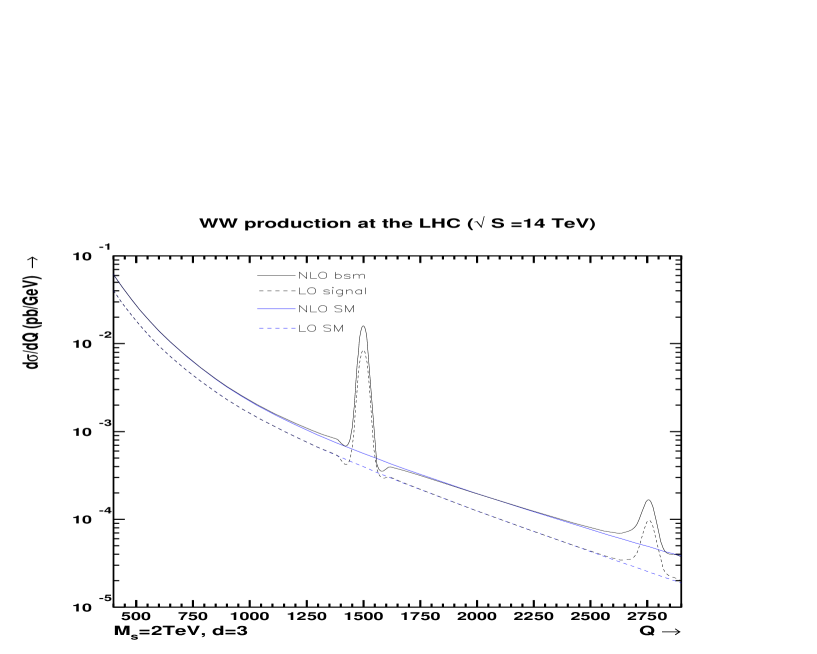
In Fig. 1 we have plotted the invariant mass distribution both for the SM and the signal for LHC at . The two curves with peaks correspond to the signal and the remaining two curves give SM predictions. Here we have chosen and . To highlight the importance of QCD corrections we have also displayed the LO results of SM and the signal, and we observe that at the factors (defined as ) has a value 1.9. Thus NLO QCD corrections give a substantial enhancement over the LO predictions.
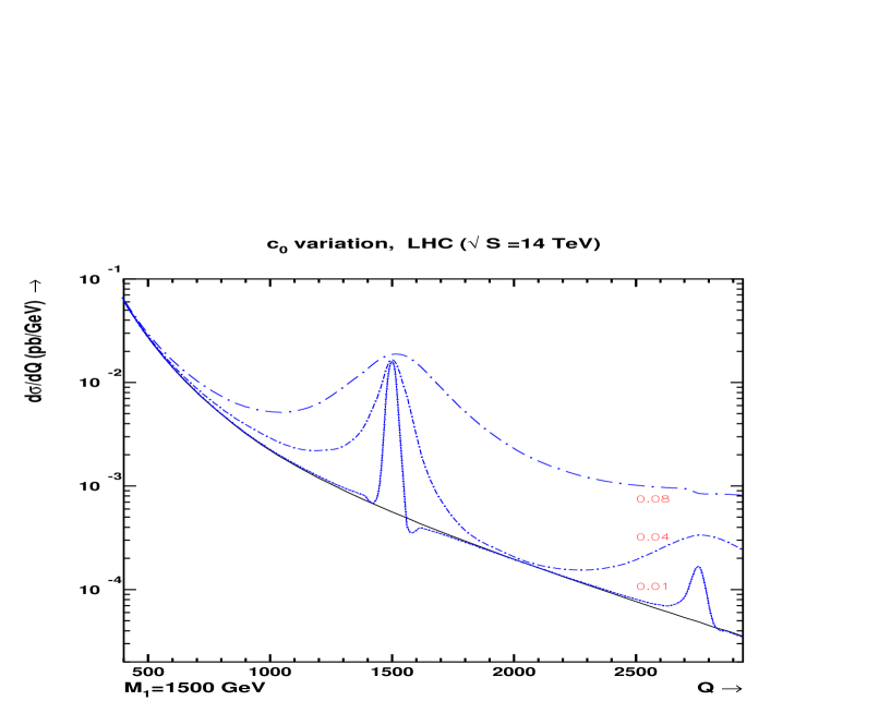
Next we present in Fig. 2 the effects of varying the parameter on the invariant mass distribution. All the curves shown correspond to NLO results, and we have also plotted the SM background for comparison.
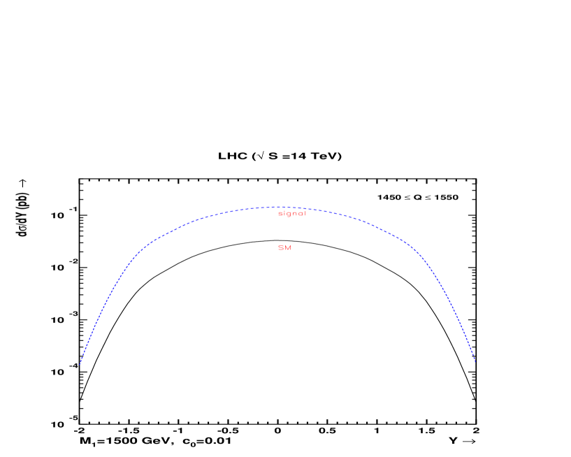
In Fig. 3 we have plotted the rapidity distribution at NLO both for SM and the signal for . We have plotted this distribution in the interval and have carried out an integration over the invariant mass interval to increase the signal over the SM background. As expected the distribution is symmetric about .
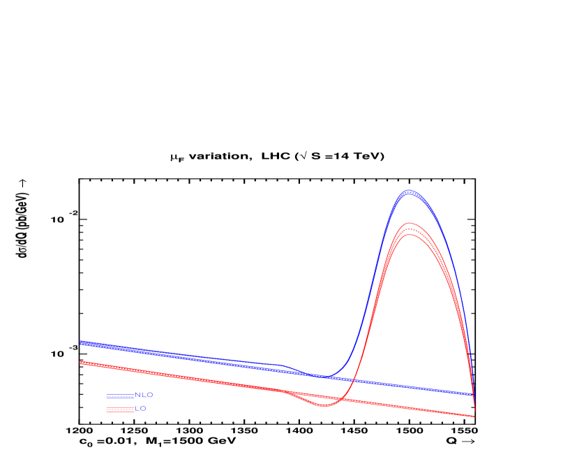
As was noted above the NLO QCD corrections reduce the sensitivity of the cross sections to the factorization scale ; this we now show in the Fig. 4. We have plotted SM and the signal both at LO and NLO, and have varied the factorization scale in the range . The central curve in a given band (shown by the dotted curves) correspond to . In all these results the renormalization scale is fixed at . We notice that the factorization scale uncertainty at LO is 21.8 % at as compared to 6.7 % at NLO. Thus we see that NLO computation achieves significant reduction in uncertainty and makes predictions much more precise.
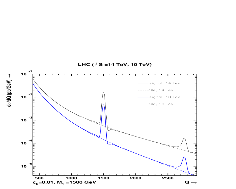
At the end we present in Fig. 5, for LHC with a centre of mass energy of at NLO both for SM and signal. For comparison we have also plotted the results in the same figure.
To summarize, in this paper we have carried out a full NLO QCD calculation for
the production of two bosons at the LHC at and in the
extra dimension model of Randall and Sundrum. Here we take all order contributions,
both in the SM and in the gravity mediated processes and their interferences,
into account.
We have presented invariant mass and rapidity distributions both at LO and NLO.
We use CTEQ 6L1 and CTEQ 6M parton density sets for LO and NLO observables, respectively.
Significant enhancements over the LO predictions are observed.
The factor are large and at (we have taken this as the first RS resonance)
. This justifies the entire exercise of carrying out a NLO computation.
The effect of variation of parameter in
invariant mass distribution is also presented. We have shown that a significant
reduction in LO theoretical uncertainty, arising from the factorization scale, is achieved
by our NLO computation. It is observed that an uncertainty of 21.8 % at LO
as is varied between and is reduced to
6.7 %.
Thus our NLO results are more precise than the LO results
and suitable for further studies for constraining the parameters of the RS model.
Invariant mass distribution is also presented for LHC at a center of mass energy of
at the NLO level.
Acknowledgments: The work of NA is supported by CSIR Senior Research Fellowship, New Delhi. NA, AT and VR would also like to thank the cluster computing facility at Harish-Chandra Research Institute. NA and VKT acknowledge the computational support of the computing facility which has been developed by the Nuclear Particle Physics Group of the Physics Department, Allahabad University under the Center of Advanced Study (CAS) funding of U.G.C. India. The authors would like to thank Prakash Mathews and M.C. Kumar for useful discussions.
References
- [1] T. Kaluza, Sitzungsber. Preuss. Akad. Wiss. Berlin (Math. Phys. ) 1921, 966 (1921); O. Klein, Z. Phys. 37, 895 (1926) [Surveys High Energ. Phys. 5, 241 (1986)].
- [2] I. Antoniadis, N. Arkani-Hamed, S. Dimopoulos and G. R. Dvali, Phys. Lett. B 436, 257 (1998) [arXiv:hep-ph/9804398]. N. Arkani-Hamed, S. Dimopoulos and G. R. Dvali, Phys. Lett. B 429, 263 (1998) [arXiv:hep-ph/9803315]. N. Arkani-Hamed, A. G. Cohen and H. Georgi, Phys. Rev. Lett. 86, 4757 (2001) [arXiv:hep-th/0104005].
- [3] L. Randall and R. Sundrum, Phys. Rev. Lett. 83, 3370 (1999) [arXiv:hep-ph/9905221]. L. Randall and R. Sundrum, Phys. Rev. Lett. 83, 4690 (1999) [arXiv:hep-th/9906064].
- [4] W. D. Goldberger and M. B. Wise, Phys. Rev. Lett. 83, 4922 (1999) [arXiv:hep-ph/9907447]; W. D. Goldberger and M. B. Wise, Phys. Lett. B 475, 275 (2000) [arXiv:hep-ph/9911457].
- [5] C. Csaki, M. Graesser, L. Randall and J. Terning, Phys. Rev. D 62, 045015 (2000) [arXiv:hep-ph/9911406]; C. Csaki, M. L. Graesser and G. D. Kribs, Phys. Rev. D 63, 065002 (2001) [arXiv:hep-th/0008151].
- [6] H. Davoudiasl, J. L. Hewett and T. G. Rizzo, Phys. Lett. B 473, 43 (2000) [arXiv:hep-ph/9911262]; A. Pomarol, Phys. Lett. B 486, 153 (2000) [arXiv:hep-ph/9911294]; S. Chang, J. Hisano, H. Nakano, N. Okada and M. Yamaguchi, Phys. Rev. D 62, 084025 (2000) [arXiv:hep-ph/9912498].
- [7] Y. Grossman and M. Neubert, Phys. Lett. B 474, 361 (2000) [arXiv:hep-ph/9912408].
- [8] T. Gherghetta and A. Pomarol, Nucl. Phys. B 586, 141 (2000) [arXiv:hep-ph/0003129].
- [9] N. Arkani-Hamed and M. Schmaltz, Phys. Rev. D 61, 033005 (2000) [arXiv:hep-ph/9903417].
- [10] S. J. Huber and Q. Shafi, Phys. Lett. B 498, 256 (2001) [arXiv:hep-ph/0010195].
- [11] S. J. Huber, Nucl. Phys. B 666, 269 (2003) [arXiv:hep-ph/0303183].
- [12] G. F. Giudice, R. Rattazzi and J. D. Wells, Nucl. Phys. B 544 (1999) 3 [arXiv:hep-ph/9811291].
- [13] T. Han, J. D. Lykken and R. J. Zhang, Phys. Rev. D 59 (1999) 105006 [arXiv:hep-ph/9811350].
- [14] P. Mathews, S. Raychaudhuri and K. Sridhar, JHEP 0007, 008 (2000) [arXiv:hep-ph/9904232]; K. Hagiwara, P. Konar, Q. Li, K. Mawatari and D. Zeppenfeld, JHEP 0804, 019 (2008) [arXiv:0801.1794 [hep-ph]]; S. Lola, P. Mathews, S. Raychaudhuri and K. Sridhar, arXiv:hep-ph/0010010; M. Kober, B. Koch and M. Bleicher, Phys. Rev. D 76, 125001 (2007) [arXiv:0708.2368 [hep-ph]]; J. Gao, C. S. Li, X. Gao and J. J. Zhang, Phys. Rev. D 80, 016008 (2009) [arXiv:0903.2551 [hep-ph]].
- [15] K. Hagiwara, R. D. Peccei, D. Zeppenfeld and K. Hikasa, Nucl. Phys. B 282 (1987) 253.
- [16] U. Baur, T. Han and J. Ohnemus, Phys. Rev. D 53, 1098 (1996) [arXiv:hep-ph/9507336].
- [17] R. W. Brown and K. O. Mikaelian, Phys. Rev. D 19 (1979) 922.
- [18] J. Ohnemus, Phys. Rev. D 44, 1403 (1991).
- [19] S. Frixione, Nucl. Phys. B 410, 280 (1993).
- [20] J. Ohnemus, Phys. Rev. D 50, 1931 (1994) [arXiv:hep-ph/9403331].
- [21] L. J. Dixon, Z. Kunszt and A. Signer, Nucl. Phys. B 531, 3 (1998) [arXiv:hep-ph/9803250].
- [22] L. J. Dixon, Z. Kunszt and A. Signer, Phys. Rev. D 60, 114037 (1999) [arXiv:hep-ph/9907305].
- [23] J. M. Campbell and R. K. Ellis, Phys. Rev. D 60, 113006 (1999) [arXiv:hep-ph/9905386].
- [24] C. Kao and D. A. Dicus, Phys. Rev. D 43, 1555 (1991); G. Davatz, G. Dissertori, M. Dittmar, M. Grazzini and F. Pauss, JHEP 0405, 009 (2004) [arXiv:hep-ph/0402218]; M. Duhrssen, K. Jakobs, J. J. van der Bij and P. Marquard, JHEP 0505, 064 (2005) [arXiv:hep-ph/0504006]; T. Binoth, M. Ciccolini, N. Kauer and M. Kramer, JHEP 0612, 046 (2006) [arXiv:hep-ph/0611170]; E. Accomando, Phys. Lett. B 661, 129 (2008) [arXiv:0709.1364 [hep-ph]].
- [25] G. Chachamis, M. Czakon and D. Eiras, arXiv:0806.3043 [hep-ph]; G. Chachamis, M. Czakon and D. Eiras, JHEP 0812, 003 (2008) [arXiv:0802.4028 [hep-ph]].
- [26] K. Agashe, H. Davoudiasl, G. Perez and A. Soni, Phys. Rev. D 76, 036006 (2007) [arXiv:hep-ph/0701186]. K. Agashe, S. Gopalakrishna, T. Han, G. Y. Huang and A. Soni, Phys. Rev. D 80, 075007 (2009) [arXiv:0810.1497 [hep-ph]]. O. Antipin, D. Atwood and A. Soni, Phys. Lett. B 666, 155 (2008) [arXiv:0711.3175 [hep-ph]].
- [27] P. Mathews, V. Ravindran, K. Sridhar and W. L. van Neerven, Nucl. Phys. B 713, 333 (2005) [arXiv:hep-ph/0411018]; P. Mathews, V. Ravindran and K. Sridhar, JHEP 0510, 031 (2005) [arXiv:hep-ph/0506158]; P. Mathews and V. Ravindran, Nucl. Phys. B 753, 1 (2006) [arXiv:hep-ph/0507250]; M. C. Kumar, P. Mathews and V. Ravindran, Eur. Phys. J. C 49, 599 (2007) [arXiv:hep-ph/0604135].
- [28] M. C. Kumar, P. Mathews, V. Ravindran and A. Tripathi, Phys. Lett. B 672, 45 (2009) [arXiv:0811.1670 [hep-ph]]; M. C. Kumar, P. Mathews, V. Ravindran and A. Tripathi, Nucl. Phys. B 818, 28 (2009) [arXiv:0902.4894 [hep-ph]].
- [29] N. Agarwal, V. Ravindran, V. K. Tiwari and A. Tripathi, arXiv:0909.2651 [hep-ph]; N. Agarwal, V. Ravindran, V. K. Tiwari and A. Tripathi, arXiv:0910.1551 [hep-ph].
- [30] X. Gao, C. S. Li, J. Gao, R. J. Oakes and J. Wang, arXiv:0912.0199 [hep-ph].
- [31] S. Karg, M. Kramer, Q. Li and D. Zeppenfeld, arXiv:0911.5095 [hep-ph].
- [32] N. Agarwal, V. Ravindran, V. K. Tiwari and A. Tripathi, under preparation.
- [33] B. W. Harris and J. F. Owens, Phys. Rev. D 65, 094032 (2002) [arXiv:hep-ph/0102128].
- [34] C. Amsler et al. [Particle Data Group], Phys. Lett. B 667, 1 (2008).
- [35] J. Pumplin, D. R. Stump, J. Huston, H. L. Lai, P. M. Nadolsky and W. K. Tung, JHEP 0207 (2002) 012 [arXiv:hep-ph/0201195]; D. Stump, J. Huston, J. Pumplin, W. K. Tung, H. L. Lai, S. Kuhlmann and J. F. Owens, JHEP 0310 (2003) 046 [arXiv:hep-ph/0303013].