Effective field theory for Sp(N) antiferromagnets
and its phase structure

Keisuke Kataoka, Shinya Hattori, and Ikuo Ichinose Department of Applied Physics, Nagoya Institute of Technology, Nagoya, Japan
Abstract

In this paper, we study quantum Sp(N) antiferromagnetic (AF) Heisenberg models in two dimensions (2D) by using the Schwinger-boson representation and the path-integral methods. An effective field theory, which is an extension of CPN-1 model in (2+1)D, is derived and its phase structure is studied by the 1/N1๐‘1/N-expansion. We introduce a spatial anisotropy in the exchange couplings and show that the effective coupling constant in the CPN-1 model is an increasing function of the anisotropy. For the SU(N) AF Heisenberg model, which is a specific case of the Sp(N) model, we found that phase transition from the ordered โ€œNรฉel stateโ€ to paramagnetic phase takes place as the anisotropy is increased. In the vicinity of the SU(N) symmetric point, this phase structure is retained. However as a parameter that controls explicit breaking of the SU(N) symmetry is increased, a new phase, which is similar to the spiral-spin phase with a nematic order in frustrated SU(2) spin systems, appears. It is shown that at that phase transition point, a local SU(2) gauge symmetry with composite SU(2) gauge field appears in the low-energy sector. It is another example of symmetry-enhancement phenomenon at low energies. We also introduce a lattice gauge-theoretical model, which is a counterpart of the effective field theory, and study its phase structure by means of the Monte-Carlo simulations.

I Introduction

Study on quantum antiferromagnets has been one of the most active area in the condensed matter physics. In particular in the last decade, much attention has been paid to exotic phase and exotic phase transition for which Landauโ€™s classic paradigm cannot be applicableglw . It is expected that investigation of such exotic states is useful to understand anomalous properties of under doped high-Tcsubscript๐‘‡๐‘T_{c} materialslnw . Furthermore recent development in technologies of ultracold atoms and optical lattice trap elevates purely academic quantum spin models to realistic ones, and these cold-atom systems are sometimes regarded as a final simulator for strongly-correlated electron systems. Quantum SU(N) antiferromagnets are one of these examples. Theoretically these models can be studied by using the Schwinger-boson methods and the 1/N1๐‘1/N-expansionrs . In a seminal papercold , it was shown that spin-(Nโˆ’1)/2๐‘12(N-1)/2 (N๐‘N is an even integer) cold atom systems in an optical lattice with one atom per quantum well can be regarded as quantum Sp(N) antiferromagnets. There are two parameters J1,J2subscript๐ฝ1subscript๐ฝ2J_{1},\;J_{2} in the Hamiltonian of the Sp(N) magnets and when J1=J2subscript๐ฝ1subscript๐ฝ2J_{1}=J_{2}, the symmetry is enhanced to SU(N)โŠƒsuperset-of\supsetSp(N) and a SU(N) quantum antiferromagnet is realized.

In the present paper, we shall study Sp(N) quantum antiferromagnets by using the slave-boson (Schwinger boson) representation and the path-integral methods. We first derive an effective field theory for the Sp(N) Heisenberg model. This field theory is an extension of the CPN-1 model for the SU(N) antiferromagnetic (AF) Heisenberg model. Then we investigate its phase structure by using the 1/N1๐‘1/N-expansion. We also study numerically its lattice-gauge-model counterpart by means of the Monte-Carlo (MC) simulations.

This paper is organized as follows. In Sect.2, we shall derive the effective field theory for the Sp(N) AF Heisenberg model by using CPN-1 representation of (pseudo-)spin degrees of freedom. In Sect.3, we study the field-theory model by the 1/N1๐‘1/N-expansion. We focus on quantum phase transition in the spatial two-dimensional (2D) system. We first show that in the SU(N) AF magnets with anisotropic exchange couplings on a square lattice, a phase transition from the AF Nรฉel state to the paramagnetic state takes place as the anisotropy is increased. These two states persist in the Sp(N) system in the vicinity of the SU(N) symmetric point J1=J2subscript๐ฝ1subscript๐ฝ2J_{1}=J_{2}. As J2/J1subscript๐ฝ2subscript๐ฝ1J_{2}/J_{1} is decreased to some critical value, a phase transition to a new phase with a composite vector-field condensation takes place and a new kind of spin order appears. In Sect.4, we study a lattice version of the obtained field theory and show the results of the numerical study for the Sp(4) case. Obtained phase diagram is qualitatively in agreement with that obtained by the 1/N1๐‘1/N-expansion, but we also find some discrepancy between the 1/N1๐‘1/N-expansion and the numerical study, e.g. order of the phase transition, etc. Section 5 is devoted for conclusion. In the Appendix, some details of the derivation of the effective field theory are given.

II Model and effective field theory

II.1 Sp(N) Heisenberg model

We consider anisotropic Sp(N) Heisenberg model on a square lattice, i.e., exchange couplings in the x๐‘ฅx and y๐‘ฆy-directions are different. Quantum Hamiltonian of the system is given as follows in the most general form,

โ„‹=โˆ‘โŸจi,jโŸฉ{J1i,jโ€‹โˆ‘a,bฮ“iaโ€‹bโ€‹ฮ“jaโ€‹bโˆ’J2i,jโ€‹โˆ‘aฮ“iaโ€‹ฮ“ja},โ„‹subscript๐‘–๐‘—subscriptsuperscript๐ฝ๐‘–๐‘—1subscript๐‘Ž๐‘subscriptsuperscriptฮ“๐‘Ž๐‘๐‘–subscriptsuperscriptฮ“๐‘Ž๐‘๐‘—subscriptsuperscript๐ฝ๐‘–๐‘—2subscript๐‘Žsubscriptsuperscriptฮ“๐‘Ž๐‘–subscriptsuperscriptฮ“๐‘Ž๐‘—{\cal H}=\sum_{\langle i,j\rangle}\Big{\{}J^{i,j}_{1}\sum_{a,b}\Gamma^{ab}_{i}\Gamma^{ab}_{j}-J^{i,j}_{2}\sum_{a}\Gamma^{a}_{i}\Gamma^{a}_{j}\Big{\}}, (2.1)

where i,j๐‘–๐‘—i,j denote lattice sites and ฮ“aโ€‹bโˆˆ๐ฌ๐ฉโ€‹(N)superscriptฮ“๐‘Ž๐‘๐ฌ๐ฉN\Gamma^{ab}\in{\bf sp}(\mathrm{N}) (the Lie algebra of Sp(N)) have Nโ€‹(N+1)2๐‘๐‘12{N(N+1)\over 2} components. On the other hand, ฮ“aโˆˆ๐ฌ๐ฎโ€‹(N)/๐ฌ๐ฉโ€‹(N)superscriptฮ“๐‘Ž๐ฌ๐ฎN๐ฌ๐ฉN\Gamma^{a}\in{\bf su}(\mathrm{N})/{\bf sp}(\mathrm{N}), and there are (N+1)โ€‹(Nโˆ’2)2๐‘1๐‘22{(N+1)(N-2)\over 2} components. Hereafter in most of cases, we set the exchange coupling J1i,jsuperscriptsubscript๐ฝ1๐‘–๐‘—J_{1}^{i,j} and J2i,jsuperscriptsubscript๐ฝ2๐‘–๐‘—J_{2}^{i,j} as follows,

Jni,i+x^=Jn,x,Jni,i+y^=Jn,y,(n=1,2),otherwiseย 0,formulae-sequencesuperscriptsubscript๐ฝ๐‘›๐‘–๐‘–^๐‘ฅsubscript๐ฝ๐‘›๐‘ฅsuperscriptsubscript๐ฝ๐‘›๐‘–๐‘–^๐‘ฆsubscript๐ฝ๐‘›๐‘ฆ๐‘›12otherwiseย 0J_{n}^{i,i+\hat{x}}=J_{n,x},\;J_{n}^{i,i+\hat{y}}=J_{n,y},\;(n=1,2),\;\mbox{otherwise $0$},

where x^โ€‹(y^)^๐‘ฅ^๐‘ฆ\hat{x}\;(\hat{y}) is the unit vector of the x๐‘ฅx(y๐‘ฆy)-direction. For the N=4๐‘4N=4 caseqi , the above generators are explicitly given as

ฮ“a=ฯƒaโŠ—ฮผz,a=1,2,3,ฮ“4=1โŠ—ฮผx,ฮ“5=1โŠ—ฮผy,formulae-sequencesuperscriptฮ“๐‘Žtensor-productsuperscript๐œŽ๐‘Žsuperscript๐œ‡๐‘งformulae-sequence๐‘Ž123formulae-sequencesuperscriptฮ“4tensor-product1superscript๐œ‡๐‘ฅsuperscriptฮ“5tensor-product1superscript๐œ‡๐‘ฆ\Gamma^{a}=\sigma^{a}\otimes\mu^{z},a=1,2,3,\;\;\Gamma^{4}=1\otimes\mu^{x},\;\;\Gamma^{5}=1\otimes\mu^{y}, (2.2)

and

ฮ“aโ€‹b=12โ€‹iโ€‹[ฮ“a,ฮ“b],superscriptฮ“๐‘Ž๐‘12๐‘–superscriptฮ“๐‘Žsuperscriptฮ“๐‘\Gamma^{ab}=\frac{1}{2i}[\Gamma^{a},\Gamma^{b}], (2.3)

where ฯƒa,ฮผaโ€‹(a=1,2,3)superscript๐œŽ๐‘Žsuperscript๐œ‡๐‘Ž๐‘Ž123\sigma^{a},\mu^{a}(a=1,2,3) are two sets of the 2ร—2222\times 2 Pauli matrices. The Sp(4) case corresponds to the spin-3/2 system, and ฮ“asuperscriptฮ“๐‘Ž\Gamma^{a} involves even powers of the SU(2) spin matrices, whereas ฮ“aโ€‹bsuperscriptฮ“๐‘Ž๐‘\Gamma^{ab} involves odd powers of the spin matrices. Then the long-range order of ฮ“asuperscriptฮ“๐‘Ž\Gamma^{a} indicates a spin-nematic order.

It is useful to introduce the matrix ๐’ฅ๐’ฅ\mathcal{J}, which has the following properties and is a generalization of the time-reversal matrix iโ€‹ฯƒ2๐‘–superscript๐œŽ2i\sigma^{2} in the SU(2) spin case,

๐’ฅt=โˆ’๐’ฅ,๐’ฅ2=โˆ’1,๐’ฅโ€‹ฮ“aโ€‹bโ€‹๐’ฅ=(ฮ“aโ€‹b)t,๐’ฅโ€‹ฮ“aโ€‹๐’ฅ=โˆ’(ฮ“a)t.formulae-sequencesuperscript๐’ฅ๐‘ก๐’ฅformulae-sequencesuperscript๐’ฅ21formulae-sequence๐’ฅsuperscriptฮ“๐‘Ž๐‘๐’ฅsuperscriptsuperscriptฮ“๐‘Ž๐‘๐‘ก๐’ฅsuperscriptฮ“๐‘Ž๐’ฅsuperscriptsuperscriptฮ“๐‘Ž๐‘ก\mathcal{J}^{t}=-\mathcal{J},\ \mathcal{J}^{2}=-1,\ \mathcal{J}\Gamma^{ab}\mathcal{J}=(\Gamma^{ab})^{t},\ \mathcal{J}\Gamma^{a}\mathcal{J}=-(\Gamma^{a})^{t}. (2.4)

For the Sp(4) case with Eqs.(2.2), ๐’ฅ=iโ€‹ฯƒyโŠ—ฮผx๐’ฅtensor-product๐‘–superscript๐œŽ๐‘ฆsuperscript๐œ‡๐‘ฅ\mathcal{J}=i\sigma^{y}\otimes\mu^{x}.

We introduce the Schwinger boson operator b^ฮฑโ€‹(ฮฑ=1,โ‹ฏ,N)subscript^๐‘๐›ผ๐›ผ1โ‹ฏ๐‘\hat{b}_{\alpha}\;(\alpha=1,\cdots,N) and represent the โ€œspin operatorsโ€ in the Hamiltonian (2.1) in terms of them, ฮ“^iaโ€‹b=b^i,ฮฑโ€ โ€‹ฮ“ฮฑโ€‹ฮฒaโ€‹bโ€‹b^i,ฮฒsubscriptsuperscript^ฮ“๐‘Ž๐‘๐‘–superscriptsubscript^๐‘๐‘–๐›ผโ€ subscriptsuperscriptฮ“๐‘Ž๐‘๐›ผ๐›ฝsubscript^๐‘๐‘–๐›ฝ\hat{\Gamma}^{ab}_{i}=\hat{b}_{i,\alpha}^{\dagger}\Gamma^{ab}_{\alpha\beta}\hat{b}_{i,\beta}, โ€„ ฮ“^ia=b^i,ฮฑโ€ โ€‹ฮ“ฮฑโ€‹ฮฒaโ€‹b^i,ฮฒ.subscriptsuperscript^ฮ“๐‘Ž๐‘–superscriptsubscript^๐‘๐‘–๐›ผโ€ subscriptsuperscriptฮ“๐‘Ž๐›ผ๐›ฝsubscript^๐‘๐‘–๐›ฝ\hat{\Gamma}^{a}_{i}=\hat{b}_{i,\alpha}^{\dagger}\Gamma^{a}_{\alpha\beta}\hat{b}_{i,\beta}. By using the identities,

โˆ‘a,bฮ“ฮฑโ€‹ฮฒaโ€‹bโ€‹ฮ“ฮณโ€‹ฯƒaโ€‹bsubscript๐‘Ž๐‘subscriptsuperscriptฮ“๐‘Ž๐‘๐›ผ๐›ฝsubscriptsuperscriptฮ“๐‘Ž๐‘๐›พ๐œŽ\displaystyle\sum_{a,b}\Gamma^{ab}_{\alpha\beta}\Gamma^{ab}_{\gamma\sigma} =2โ€‹ฮดฮฑโ€‹ฯƒโ€‹ฮดฮฒโ€‹ฮณโˆ’2โ€‹๐’ฅฮฑโ€‹ฮณโ€‹๐’ฅฮฒโ€‹ฯƒ,absent2subscript๐›ฟ๐›ผ๐œŽsubscript๐›ฟ๐›ฝ๐›พ2subscript๐’ฅ๐›ผ๐›พsubscript๐’ฅ๐›ฝ๐œŽ\displaystyle=2\delta_{\alpha\sigma}\delta_{\beta\gamma}-2\mathcal{J}_{\alpha\gamma}\mathcal{J}_{\beta\sigma}, (2.5)
โˆ‘aฮ“ฮฑโ€‹ฮฒaโ€‹ฮ“ฮณโ€‹ฯƒasubscript๐‘Žsubscriptsuperscriptฮ“๐‘Ž๐›ผ๐›ฝsubscriptsuperscriptฮ“๐‘Ž๐›พ๐œŽ\displaystyle\sum_{a}\Gamma^{a}_{\alpha\beta}\Gamma^{a}_{\gamma\sigma} =2โ€‹ฮดฮฑโ€‹ฯƒโ€‹ฮดฮฒโ€‹ฮณ+2โ€‹๐’ฅฮฑโ€‹ฮณโ€‹๐’ฅฮฒโ€‹ฯƒโˆ’ฮดฮฑโ€‹ฮฒโ€‹ฮดฮณโ€‹ฯƒ,absent2subscript๐›ฟ๐›ผ๐œŽsubscript๐›ฟ๐›ฝ๐›พ2subscript๐’ฅ๐›ผ๐›พsubscript๐’ฅ๐›ฝ๐œŽsubscript๐›ฟ๐›ผ๐›ฝsubscript๐›ฟ๐›พ๐œŽ\displaystyle=2\delta_{\alpha\sigma}\delta_{\beta\gamma}+2\mathcal{J}_{\alpha\gamma}\mathcal{J}_{\beta\sigma}-\delta_{\alpha\beta}\delta_{\gamma\sigma}, (2.6)

we obtain

โ„‹=โˆ‘โŸจi,jโŸฉ{2โ€‹(J1i,jโˆ’J2i,j)โ€‹K^iโ€‹jโ€ โ€‹K^iโ€‹jโˆ’2โ€‹(J1i,j+J2i,j)โ€‹Q^iโ€‹jโ€ โ€‹Q^iโ€‹j},โ„‹subscript๐‘–๐‘—2superscriptsubscript๐ฝ1๐‘–๐‘—superscriptsubscript๐ฝ2๐‘–๐‘—superscriptsubscript^๐พ๐‘–๐‘—โ€ subscript^๐พ๐‘–๐‘—2superscriptsubscript๐ฝ1๐‘–๐‘—superscriptsubscript๐ฝ2๐‘–๐‘—superscriptsubscript^๐‘„๐‘–๐‘—โ€ subscript^๐‘„๐‘–๐‘—\mathcal{H}=\sum_{\langle i,j\rangle}\{2(J_{1}^{i,j}-J_{2}^{i,j})\hat{K}_{ij}^{\dagger}\hat{K}_{ij}-2(J_{1}^{i,j}+J_{2}^{i,j})\hat{Q}_{ij}^{\dagger}\hat{Q}_{ij}\}, (2.7)

where Q^iโ€‹j=๐’ฅฮฑโ€‹ฮฒโ€‹b^i,ฮฑโ€‹b^j,ฮฒsubscript^๐‘„๐‘–๐‘—subscript๐’ฅ๐›ผ๐›ฝsubscript^๐‘๐‘–๐›ผsubscript^๐‘๐‘—๐›ฝ\hat{Q}_{ij}=\mathcal{J}_{\alpha\beta}\hat{b}_{i,\alpha}\hat{b}_{j,\beta} and K^iโ€‹j=b^ฮฑ,iโ€ โ€‹b^ฮฑ,jsubscript^๐พ๐‘–๐‘—subscriptsuperscript^๐‘โ€ ๐›ผ๐‘–subscript^๐‘๐›ผ๐‘—\hat{K}_{ij}=\hat{b}^{\dagger}_{\alpha,i}\hat{b}_{\alpha,j}. The operator ๐’ฅฮฑโ€‹ฮฒโ€‹b^j,ฮฒsubscript๐’ฅ๐›ผ๐›ฝsubscript^๐‘๐‘—๐›ฝ\mathcal{J}_{\alpha\beta}\hat{b}_{j,\beta} is the conjugate spinor of b^j,ฮฒsubscript^๐‘๐‘—๐›ฝ\hat{b}_{j,\beta} and then Q^iโ€‹jsubscript^๐‘„๐‘–๐‘—\hat{Q}_{ij} represents pairing of spins on the lattice sites i,j๐‘–๐‘—i,j, whereas K^iโ€‹jsubscript^๐พ๐‘–๐‘—\hat{K}_{ij} corresponds to the Schwinger boson (spinon) hopping. Subsidiary condition

โˆ‘ฮฑ=1Nb^i,ฮฑโ€ โ€‹b^i,ฮฑโ€‹|physโŸฉ=|physโŸฉ,superscriptsubscript๐›ผ1๐‘subscriptsuperscript^๐‘โ€ ๐‘–๐›ผsubscript^๐‘๐‘–๐›ผketphysketphys\sum_{\alpha=1}^{N}\hat{b}^{\dagger}_{i,\alpha}\hat{b}_{i,\alpha}|\mbox{phys}\rangle=|\mbox{phys}\rangle, (2.8)

must be imposed as the physical-state condition. We redefine the exchange couplings as Ji,jโ‰ก2โ€‹(J1i,j+J2i,j)subscript๐ฝ๐‘–๐‘—2superscriptsubscript๐ฝ1๐‘–๐‘—superscriptsubscript๐ฝ2๐‘–๐‘—J_{i,j}\equiv 2(J_{1}^{i,j}+J_{2}^{i,j}), Ji,jโ€ฒโ‰ก2โ€‹(J1i,jโˆ’J2i,j)subscriptsuperscript๐ฝโ€ฒ๐‘–๐‘—2superscriptsubscript๐ฝ1๐‘–๐‘—superscriptsubscript๐ฝ2๐‘–๐‘—J^{\prime}_{i,j}\equiv 2(J_{1}^{i,j}-J_{2}^{i,j}), then

โ„‹=โˆ‘โŸจi,jโŸฉ{Ji,jโ€ฒโ€‹K^iโ€‹jโ€ โ€‹K^iโ€‹jโˆ’Ji,jโ€‹Q^iโ€‹jโ€ โ€‹Q^iโ€‹j}.โ„‹subscript๐‘–๐‘—subscriptsuperscript๐ฝโ€ฒ๐‘–๐‘—superscriptsubscript^๐พ๐‘–๐‘—โ€ subscript^๐พ๐‘–๐‘—subscript๐ฝ๐‘–๐‘—superscriptsubscript^๐‘„๐‘–๐‘—โ€ subscript^๐‘„๐‘–๐‘—{\cal H}=\sum_{\langle i,j\rangle}\{J^{\prime}_{i,j}\hat{K}_{ij}^{\dagger}\hat{K}_{ij}-J_{i,j}\hat{Q}_{ij}^{\dagger}\hat{Q}_{ij}\}. (2.9)

From Eq.(2.9), it is obvious that when Ji,jโ€ฒ=0subscriptsuperscript๐ฝโ€ฒ๐‘–๐‘—0J^{\prime}_{i,j}=0 (Ji,j=0subscript๐ฝ๐‘–๐‘—0J_{i,j}=0), the model have the global SU(N) symmetry. In the following section, we shall derive the effective field theory for the system (2.9) by using the path-integral methods.

II.2 Effective field theory

In this subsection, we shall derive the low-energy effective field theory of the Hamiltonian (2.9). To this end, we use the coherent path-integral methods. For the Schwinger boson, we use the CPN-1 boson that satisfies zยฏiโ‹…zi=โˆ‘ฮฑzยฏi,ฮฑโ€‹zi,ฮฑ=1โ‹…subscriptยฏ๐‘ง๐‘–subscript๐‘ง๐‘–subscript๐›ผsubscriptยฏ๐‘ง๐‘–๐›ผsubscript๐‘ง๐‘–๐›ผ1\bar{z}_{i}\cdot z_{i}=\sum_{\alpha}\bar{z}_{i,\alpha}z_{i,\alpha}=1 corresponding to the condition (2.8). Then the partition function is given as

Z๐‘\displaystyle Z =โˆซ๐’Ÿโ€‹zยฏโ€‹๐’Ÿโ€‹zโ€‹ฮดโ€‹(zยฏโ‹…zโˆ’1)โ€‹expโก[โˆซ0ฮฒ๐‘‘ฯ„โ€‹Aโ€‹(ฯ„)]absent๐’Ÿยฏ๐‘ง๐’Ÿ๐‘ง๐›ฟโ‹…ยฏ๐‘ง๐‘ง1subscriptsuperscript๐›ฝ0differential-d๐œ๐ด๐œ\displaystyle=\int\mathcal{D}\bar{z}\mathcal{D}z\delta(\bar{z}\cdot z-1)\exp\left[\int^{\beta}_{0}d\tau A(\tau)\right]
Aโ€‹(ฯ„)๐ด๐œ\displaystyle A(\tau) =โˆ’โˆ‘i,ฮฑzยฏi,ฮฑโ€‹zห™i,ฮฑโˆ’โ„‹โ€‹(z,zยฏ),absentsubscript๐‘–๐›ผsubscriptยฏ๐‘ง๐‘–๐›ผsubscriptห™๐‘ง๐‘–๐›ผโ„‹๐‘งยฏ๐‘ง\displaystyle=-\sum_{i,\alpha}\bar{z}_{i,\alpha}\dot{z}_{i,\alpha}-\mathcal{H}(z,\bar{z}), (2.10)

where โ„‹โ€‹(z,zยฏ)โ„‹๐‘งยฏ๐‘ง\mathcal{H}(z,\bar{z}) is obtained from Eq.(2.9) by replacing b^i,ฮฑโ†’zi,ฮฑโ†’subscript^๐‘๐‘–๐›ผsubscript๐‘ง๐‘–๐›ผ\hat{b}_{i,\alpha}\rightarrow{z}_{i,\alpha} and b^i,ฮฑโ€ โ†’zยฏi,ฮฑโ†’subscriptsuperscript^๐‘โ€ ๐‘–๐›ผsubscriptยฏ๐‘ง๐‘–๐›ผ\hat{b}^{\dagger}_{i,\alpha}\rightarrow\bar{z}_{i,\alpha}.

Refer to caption
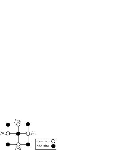
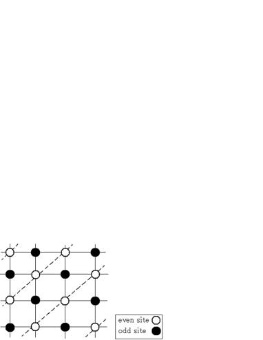
Figure 1: CP1 variables on odd sites are paired with their NN zesubscript๐‘ง๐‘’z_{e}.

In order to obtain the effective field theory from Eq.(2.10), we integrate out the half of the CPN-1 variables, e.g. those at odd sitesim . To this end, we introduce a complete-orthogonal set of vectors in the CPN-1 space, {wi;i=0,1,โ‹ฏ,Nโˆ’1}formulae-sequencesubscript๐‘ค๐‘–๐‘–01โ‹ฏ๐‘1\{w_{i};i=0,1,\cdots,N-1\}. Arbitrary CPN-1 variable z๐‘งz can be expanded as z=โˆ‘ipiโ€‹wi๐‘งsubscript๐‘–subscript๐‘๐‘–subscript๐‘ค๐‘–z=\sum_{i}p_{i}w_{i}, where pisubscript๐‘๐‘–p_{i}โ€™s are complex numbers satisfying โˆ‘i|pi|2=1subscript๐‘–superscriptsubscript๐‘๐‘–21\sum_{i}|p_{i}|^{2}=1. As we are interested in the case with the both exchange couplings Ji,j,Ji,jโ€ฒโ‰ฅ0subscript๐ฝ๐‘–๐‘—subscriptsuperscript๐ฝโ€ฒ๐‘–๐‘—0J_{i,j},\;J^{\prime}_{i,j}\geq 0, dominant configurations in the path integral are given by zeโ‰ˆzsubscript๐‘ง๐‘’๐‘งz_{e}\approx z at even sites and zoโ‰ˆ๐’ฅโ€‹zยฏsubscript๐‘ง๐‘œ๐’ฅยฏ๐‘งz_{o}\approx\mathcal{J}\bar{z} at odd sites, where z๐‘งz is a smoothly varying CPN-1 field. We parameterize odd-site zosubscript๐‘ง๐‘œz_{o} by referring to one of its nearest-neighbor(NN) even sites zesubscript๐‘ง๐‘’z_{e} as (see Fig.1),

zo=โˆ‘ipiโ€‹wi,subscript๐‘ง๐‘œsubscript๐‘–subscript๐‘๐‘–subscript๐‘ค๐‘–z_{o}=\sum_{i}p_{i}w_{i}, (2.11)

where w0=ze,w1=๐’ฅโ€‹zยฏeformulae-sequencesubscript๐‘ค0subscript๐‘ง๐‘’subscript๐‘ค1๐’ฅsubscriptยฏ๐‘ง๐‘’w_{0}=z_{e},\;w_{1}=\mathcal{J}\bar{z}_{e} and we do not have to specify the other wisubscript๐‘ค๐‘–w_{i}โ€™s. Then by the above remarks on the dominant configurations, we can assume piโ€‹(iโ‰ 1)โ‰ช1much-less-thansubscript๐‘๐‘–๐‘–11p_{i}(i\neq 1)\ll 1 and

p1subscript๐‘1\displaystyle p_{1} =Uโ€‹(1โˆ’โˆ‘iโ‰ 1|pi|2)1/2absent๐‘ˆsuperscript1subscript๐‘–1superscriptsubscript๐‘๐‘–212\displaystyle=U(1-\sum_{i\neq 1}|p_{i}|^{2})^{1/2}
โ‰ˆUโˆ’12โ€‹Uโ€‹(โˆ‘iโ‰ 1|pi|2),absent๐‘ˆ12๐‘ˆsubscript๐‘–1superscriptsubscript๐‘๐‘–2\displaystyle\approx U-\frac{1}{2}U(\sum_{i\neq 1}|p_{i}|^{2}), (2.12)

where U๐‘ˆU is a U(1) variable that appears as a result of the local U(1) symmetry of the system, zi,ฮฑโ†’eiโ€‹ฮธiโ€‹zi,ฮฑโ†’subscript๐‘ง๐‘–๐›ผsuperscript๐‘’๐‘–subscript๐œƒ๐‘–subscript๐‘ง๐‘–๐›ผz_{i,\alpha}\rightarrow e^{i\theta_{i}}z_{i,\alpha}.

From Eq.(2.12),

zoโ‰ˆโˆ‘iโ‰ 1piโ€‹wi+Uโ€‹(1โˆ’12โ€‹โˆ‘iโ‰ 1|pi|2)โ€‹w1.subscript๐‘ง๐‘œsubscript๐‘–1subscript๐‘๐‘–subscript๐‘ค๐‘–๐‘ˆ112subscript๐‘–1superscriptsubscript๐‘๐‘–2subscript๐‘ค1z_{o}\approx\sum_{i\neq 1}p_{i}w_{i}+U\left(1-\dfrac{1}{2}\sum_{i\neq 1}|p_{i}|^{2}\right)w_{1}. (2.13)

By substituting Eq.(2.13) into the action (2.10), we obtain

Aโ€‹(ฯ„)=โˆ‘oddโˆ’site(A0+๐ฉยฏโ‹…๐ค+๐ฅยฏโ‹…๐ฉโˆ’๐ฉยฏโ€‹๐Œ๐ฉ)+Oโ€‹(๐ฉ4),๐ด๐œsubscriptoddsitesubscript๐ด0โ‹…ยฏ๐ฉ๐คโ‹…ยฏ๐ฅ๐ฉยฏ๐ฉ๐Œ๐ฉ๐‘‚superscript๐ฉ4\displaystyle A(\tau)=\sum_{\rm odd-site}(A_{0}+\bar{\mathbf{p}}\cdot\mathbf{k}+\bar{\mathbf{l}}\cdot\mathbf{p}-\bar{\mathbf{p}}\mathbf{M}\mathbf{p})+O(\mathbf{p}^{4}), (2.14)

where ๐ฉ=(p0,p2,p3,โ‹ฏ,pNโˆ’1)t๐ฉsuperscriptsubscript๐‘0subscript๐‘2subscript๐‘3โ‹ฏsubscript๐‘๐‘1๐‘ก\mathbf{p}=(p_{0},p_{2},p_{3},\cdots,p_{N-1})^{t}. The matrix ๐Œ๐Œ\mathbf{M} is explicitly given as follows,

๐Œ=(โˆ’4โ€‹Jo,jโˆ’4โ€‹Jo,jโ€ฒ0โ‹ฏ00โˆ’4โ€‹Jo,jโ‹ฏ0โ‹…0โ‹…โ‹…โ‹…โ‹…โ‹…000โ‹ฏโˆ’4โ€‹Jo,j)๐Œ4subscript๐ฝ๐‘œ๐‘—4subscriptsuperscript๐ฝโ€ฒ๐‘œ๐‘—0โ‹ฏ004subscript๐ฝ๐‘œ๐‘—โ‹ฏ0โ‹…0โ‹…โ‹…โ‹…โ‹…โ‹…000โ‹ฏ4subscript๐ฝ๐‘œ๐‘—\mathbf{M}=\left(\begin{array}[]{cccc}-4J_{o,j}-4J^{\prime}_{o,j}&0&\cdots&0\\ 0&-4J_{o,j}&\cdots&0\\ \cdot&0&\cdot&\cdot\\ \cdot&\cdot&\cdot&0\\ 0&0&\cdots&-4J_{o,j}\end{array}\right) (2.15)

and the โ€œvectorsโ€ ๐ค๐ค\mathbf{k} and ๐ฅยฏยฏ๐ฅ\bar{\mathbf{l}} have rather complicated form of composite of z๐‘งz, zยฏยฏ๐‘ง\bar{z}, w๐‘คw and wยฏยฏ๐‘ค\bar{w}, which are explicitly shown in the Appendix. In Eq.(2.15), Jo,jโ€‹(Jo,jโ€ฒ)subscript๐ฝ๐‘œ๐‘—subscriptsuperscript๐ฝโ€ฒ๐‘œ๐‘—J_{o,j}\;(J^{\prime}_{o,j}) denotes Ji,jโ€‹(Ji,jโ€ฒ)subscript๐ฝ๐‘–๐‘—subscriptsuperscript๐ฝโ€ฒ๐‘–๐‘—J_{i,j}\;(J^{\prime}_{i,j}) for i=o๐‘–๐‘œi=o and the NN even j๐‘—j (see Fig.2). As the kernel ๐Œ๐Œ\mathbf{M} has negative diagonal elements, the Gaussian integral over ๐ฉ๐ฉ\mathbf{p} can be safely done,

Z๐‘\displaystyle Z =โˆซ๐’Ÿโ€‹zยฏโ€‹๐’Ÿโ€‹zโ€‹ฮดโ€‹(zยฏโ‹…zโˆ’1)โ€‹expโก[โˆซ0ฮฒ๐‘‘ฯ„โ€‹Aโ€‹(ฯ„)]absent๐’Ÿยฏ๐‘ง๐’Ÿ๐‘ง๐›ฟโ‹…ยฏ๐‘ง๐‘ง1subscriptsuperscript๐›ฝ0differential-d๐œ๐ด๐œ\displaystyle=\int\mathcal{D}\bar{z}\mathcal{D}z\delta(\bar{z}\cdot z-1)\exp\left[\int^{\beta}_{0}d\tau A(\tau)\right]
=โˆซ๐’Ÿโ€‹๐ฉยฏโ€‹๐’Ÿโ€‹๐ฉโ€‹expโก[โˆซ0ฮฒ๐‘‘ฯ„โ€‹Aโ€‹(ฯ„)]absent๐’Ÿยฏ๐ฉ๐’Ÿ๐ฉsubscriptsuperscript๐›ฝ0differential-d๐œ๐ด๐œ\displaystyle=\int\mathcal{D}\bar{\mathbf{p}}\mathcal{D}\mathbf{p}\exp\left[\int^{\beta}_{0}d\tau A(\tau)\right]
โ‰ˆexpโก[โˆซ0ฮฒ๐‘‘ฯ„โ€‹Azโ€‹(ฯ„)],absentsuperscriptsubscript0๐›ฝdifferential-d๐œsubscript๐ด๐‘ง๐œ\displaystyle\approx\exp\bigg{[}\int_{0}^{\beta}d\tau A_{z}(\tau)\bigg{]}, (2.16)
Azโ€‹(ฯ„)=โˆ‘oddโˆ’site๐ฅยฏโ€‹(ฯ„)โ€‹๐Œโˆ’1โ€‹(ฯ„)โ€‹๐คโ€‹(ฯ„)+โˆ‘oddโˆ’siteA0โ€‹(ฯ„),subscript๐ด๐‘ง๐œsubscriptoddsiteยฏ๐ฅ๐œsuperscript๐Œ1๐œ๐ค๐œsubscriptoddsitesubscript๐ด0๐œA_{z}(\tau)=\sum_{\mathrm{odd-site}}\bar{\bf{l}}(\tau){\bf{M}}^{-1}(\tau){\bf{k}}(\tau)+\sum_{\mathrm{odd-site}}A_{0}(\tau), (2.17)
A0=โˆ’โˆ‘jJo,jโ€‹(zยฏjโ€‹๐’ฅโ€‹wยฏ1)โ€‹(zjโ€‹๐’ฅโ€‹w1)โˆ’โˆ‘jJo,jโ€ฒโ€‹(wยฏ1โ€‹zj)โ€‹(zยฏjโ€‹w1),subscript๐ด0subscript๐‘—subscript๐ฝ๐‘œ๐‘—subscriptยฏ๐‘ง๐‘—๐’ฅsubscriptยฏ๐‘ค1subscript๐‘ง๐‘—๐’ฅsubscript๐‘ค1subscript๐‘—subscriptsuperscript๐ฝโ€ฒ๐‘œ๐‘—subscriptยฏ๐‘ค1subscript๐‘ง๐‘—subscriptยฏ๐‘ง๐‘—subscript๐‘ค1A_{0}=-\sum_{j}J_{o,j}(\bar{z}_{j}\mathcal{J}\bar{w}_{1})(z_{j}\mathcal{J}w_{1})-\sum_{j}J^{\prime}_{o,j}(\bar{w}_{1}z_{j})(\bar{z}_{j}{w}_{1}), (2.18)

where โˆ‘jsubscript๐‘—\sum_{j} in Eq.(2.18) denotes the summation over even site j๐‘—j around odd site o๐‘œo (see Fig.2).

Refer to caption
Figure 2: zosubscript๐‘ง๐‘œz_{o} and its NN zjsubscript๐‘ง๐‘—z_{j}โ€™s on even sites.

We can consider a continuum limit of the effective model (2.17), as the remaining variables zjsubscript๐‘ง๐‘—z_{j}โ€™s can be regarded as a smoothly varying field zโ€‹(r)๐‘ง๐‘Ÿz(r) (r0=ฯ„,r1=x,r2=yformulae-sequencesubscript๐‘Ÿ0๐œformulae-sequencesubscript๐‘Ÿ1๐‘ฅsubscript๐‘Ÿ2๐‘ฆr_{0}=\tau,r_{1}=x,r_{2}=y). Hereafter we explicitly set the exchange couplings between adjacent spins as follows,

Jx=J0,Jy=ฮปโ€‹J0,Jxโ€ฒ=J0โ€ฒ,Jyโ€ฒ=ฮปโ€‹J0โ€ฒ,formulae-sequencesubscript๐ฝ๐‘ฅsubscript๐ฝ0formulae-sequencesubscript๐ฝ๐‘ฆ๐œ†subscript๐ฝ0formulae-sequencesubscriptsuperscript๐ฝโ€ฒ๐‘ฅsubscriptsuperscript๐ฝโ€ฒ0subscriptsuperscript๐ฝโ€ฒ๐‘ฆ๐œ†subscriptsuperscript๐ฝโ€ฒ0J_{x}=J_{0},\ J_{y}=\lambda J_{0},\ J^{\prime}_{x}=J^{\prime}_{0},\ J^{\prime}_{y}=\lambda J^{\prime}_{0}, (2.19)

where ฮป๐œ†\lambda is the parameter for the anisotropy between x๐‘ฅx and y๐‘ฆy directions. We take the limit ฮฒ=1Tโ†’โˆž๐›ฝ1๐‘‡โ†’\beta={1\over T}\rightarrow\infty, introduce explicitly the lattice spacing a๐‘Ža and rescale the coordinates as,

{ฯ„โ†’2โ€‹(1+ฮป)โ€‹J0โ€‹aโ€‹ฯ„=cโ€‹ฯ„xโ†’1+ฮป2โ€‹xyโ†’1+ฮป2โ€‹ฮปโ€‹y,casesโ†’๐œ21๐œ†subscript๐ฝ0๐‘Ž๐œ๐‘๐œotherwiseโ†’๐‘ฅ1๐œ†2๐‘ฅotherwiseโ†’๐‘ฆ1๐œ†2๐œ†๐‘ฆotherwise\displaystyle\begin{cases}\tau\rightarrow\sqrt{2}(1+\lambda)J_{0}a\tau=c\tau\\ x\rightarrow\sqrt{\frac{1+\lambda}{2}}x\\ y\rightarrow\sqrt{\frac{1+\lambda}{2\lambda}}y,\end{cases} (2.20)

where c๐‘c is the โ€œspeed of lightโ€ of the system. Then we obtain action of the effective field theory for anisotropic Sp(N) AF magnets in two dimensions,

S=12โ€‹gโ€‹โˆซd3โ€‹rโ€‹(Dฮผโ€‹zยฏโ€‹Dฮผโ€‹zโˆ’ฮณโ€‹(zยฏโ€‹๐’ฅโ€‹Dฮผโ€‹zยฏ)โ€‹(zโ€‹๐’ฅโ€‹Dฮผโ€‹z)+ฯƒโ€‹(|z|2โˆ’1)),๐‘†12๐‘”superscript๐‘‘3๐‘Ÿsubscript๐ท๐œ‡ยฏ๐‘งsubscript๐ท๐œ‡๐‘ง๐›พยฏ๐‘ง๐’ฅsubscript๐ท๐œ‡ยฏ๐‘ง๐‘ง๐’ฅsubscript๐ท๐œ‡๐‘ง๐œŽsuperscript๐‘ง21S=\frac{1}{2g}\int d^{3}r\Big{(}D_{\mu}\bar{z}D_{\mu}z-\gamma(\bar{z}\mathcal{J}D_{\mu}\bar{z})(z\mathcal{J}D_{\mu}z)+\sigma(|z|^{2}-1)\Big{)}, (2.21)

where Dฮผ=โˆ‚ฮผโˆ’zยฏโ€‹โˆ‚ฮผzsubscript๐ท๐œ‡subscript๐œ‡ยฏ๐‘งsubscript๐œ‡๐‘งD_{\mu}=\partial_{\mu}-\bar{z}\partial_{\mu}z, ฯƒ๐œŽ\sigma is the Lagrange multiplier for the CPN-1 constraint, ฮณ๐›พ\gamma is an increasing function of J0โ€ฒ/J0subscriptsuperscript๐ฝโ€ฒ0subscript๐ฝ0J^{\prime}_{0}/J_{0}, ฮณ=J0โ€ฒ/J0+Oโ€‹((J0โ€ฒ/J0)2)๐›พsubscriptsuperscript๐ฝโ€ฒ0subscript๐ฝ0๐‘‚superscriptsubscriptsuperscript๐ฝโ€ฒ0subscript๐ฝ02\gamma=J^{\prime}_{0}/J_{0}+O((J^{\prime}_{0}/J_{0})^{2}), and the coupling constant g๐‘”g is given by

g=1+ฮป2โ€‹ฮปโ€‹a.๐‘”1๐œ†2๐œ†๐‘Žg=\frac{1+\lambda}{\sqrt{2\lambda}}a. (2.22)

From Eq.(2.22), it is obvious that the effective coupling g๐‘”g has the minimum at the isotropic point ฮป=1๐œ†1\lambda=1. As we see in the following section, this means that the anisotropy tends to break the AF order of the ground state.

As it is shown in the Appendix, there also exists a Berry phase in the action,

SB=โˆ’16โ€‹2โ€‹ฮป1+ฮปโ€‹(1โˆ’J0โ€ฒJ0)โ€‹โˆซd3โ€‹rโ€‹ฯตฮผโ€‹ฮฝโ€‹ฯโ€‹Dฮผโ€‹(Dยฏฮฝโ€‹zยฏโ€‹Dฯโ€‹z).subscript๐‘†๐ต162๐œ†1๐œ†1subscriptsuperscript๐ฝโ€ฒ0subscript๐ฝ0superscript๐‘‘3๐‘Ÿsubscriptitalic-ฯต๐œ‡๐œˆ๐œŒsubscript๐ท๐œ‡subscriptยฏ๐ท๐œˆยฏ๐‘งsubscript๐ท๐œŒ๐‘งS_{B}=-\frac{1}{6}\sqrt{\frac{2\lambda}{1+\lambda}}\Big{(}1-{J^{\prime}_{0}\over J_{0}}\Big{)}\int d^{3}r\epsilon_{\mu\nu\rho}D_{\mu}(\bar{D}_{\nu}\bar{z}D_{\rho}z). (2.23)

The Berry phase (2.23) with the fractional coefficient depending on the anisotropy ฮป๐œ†\lambda and Jโ€ฒsuperscript๐ฝโ€ฒJ^{\prime}-coupling does not suppress effects of instanton in contrast to that with an integer coefficient, i.e., SBsubscript๐‘†๐ตS_{B} does not give any substantial effects on the phase structure and critical behavioryoshioka . For the case of the SU(2) AF magnets on 2D lattice with anisotropic couplings, this observation has been verified directly by the numerical studyJanke .

In the following sections, we shall study the field theory (2.21) by analytical and numerical methods.

III Phase structure: Analytical study

III.1 1/N1๐‘1/N expansion: Case of small ฮณ๐›พ\gamma

The partition function of the effective field theory is given as,

Z=โˆซ๐’Ÿโ€‹zโ€‹๐’Ÿโ€‹zยฏโ€‹๐’Ÿโ€‹ฯƒโ€‹expโก(โˆ’N2โ€‹gโ€‹โˆซd3โ€‹rโ€‹[Dฮผโ€‹zยฏโ€‹Dฮผโ€‹zโˆ’ฮณโ€‹(zยฏโ€‹๐’ฅโ€‹Dฮผโ€‹zยฏ)โ€‹(zโ€‹๐’ฅโ€‹Dฮผโ€‹z)+ฯƒโ€‹(|z|2โˆ’1)]),๐‘๐’Ÿ๐‘ง๐’Ÿยฏ๐‘ง๐’Ÿ๐œŽ๐‘2๐‘”superscript๐‘‘3๐‘Ÿdelimited-[]subscript๐ท๐œ‡ยฏ๐‘งsubscript๐ท๐œ‡๐‘ง๐›พยฏ๐‘ง๐’ฅsubscript๐ท๐œ‡ยฏ๐‘ง๐‘ง๐’ฅsubscript๐ท๐œ‡๐‘ง๐œŽsuperscript๐‘ง21\displaystyle Z=\int\mathcal{D}z\mathcal{D}\bar{z}\mathcal{D}\sigma\exp\Big{(}-\frac{N}{2g}\int d^{3}r[D_{\mu}\bar{z}D_{\mu}z-\gamma(\bar{z}\mathcal{J}D_{\mu}\bar{z})(z\mathcal{J}D_{\mu}z)\;\;+\sigma(|z|^{2}-1)]\Big{)}, (3.1)

where we have introduced the factor N๐‘N in front of the action to perform the 1/N1๐‘1/N-expansion in the analytical studyan . At ฮณ=0๐›พ0\gamma=0, the system (3.1) has the global SU(N) symmetry, z(r)โ†’Vz(r),Vโˆˆz(r)\rightarrow Vz(r),\;V\in SU(N). We first consider the case of small ฮณ๐›พ\gamma, and put the following parameterization for z๐‘งz, z=z0+u+iโ€‹v,๐‘งsubscript๐‘ง0๐‘ข๐‘–๐‘ฃz=z_{0}+u+iv, where z0=(n0,0,โ‹ฏ,0),u=(0,u2,โ‹ฏ,uN)โ€‹andโ€‹v=(0,v2,โ‹ฏ,vN).formulae-sequencesubscript๐‘ง0subscript๐‘›00โ‹ฏ0๐‘ข0subscript๐‘ข2โ‹ฏsubscript๐‘ข๐‘and๐‘ฃ0subscript๐‘ฃ2โ‹ฏsubscript๐‘ฃ๐‘z_{0}=(n_{0},0,\cdots,0),\;u=(0,u_{2},\cdots,u_{N})\;\mbox{and}\;v=(0,v_{2},\cdots,v_{N}). The fields u๐‘ขu and v๐‘ฃv are real vectors. We have used the gauge-fixing condition v1=0subscript๐‘ฃ10v_{1}=0. After substituting the above parameterization to Eq.(3.1) and keeping the quadratic terms, we perform the Gaussian integration over u๐‘ขu and v๐‘ฃv as the leading order of 1/N1๐‘1/N,

Z๐‘\displaystyle Z =โˆซ๐’Ÿโ€‹n0โ€‹๐’Ÿโ€‹ฯƒโ€‹๐’Ÿโ€‹uโ€‹๐’Ÿโ€‹vโ€‹expโก[โˆ’N2โ€‹gโ€‹โˆซd3โ€‹rโ€‹{(โˆ‚ฮผu)2+(โˆ‚ฮผv)2+ฯƒโ€‹(n02+u2+v2โˆ’1)}]absent๐’Ÿsubscript๐‘›0๐’Ÿ๐œŽ๐’Ÿ๐‘ข๐’Ÿ๐‘ฃ๐‘2๐‘”superscript๐‘‘3๐‘Ÿsuperscriptsubscript๐œ‡๐‘ข2superscriptsubscript๐œ‡๐‘ฃ2๐œŽsuperscriptsubscript๐‘›02superscript๐‘ข2superscript๐‘ฃ21\displaystyle=\int\mathcal{D}n_{0}\mathcal{D}\sigma\mathcal{D}u\mathcal{D}v\exp\Big{[}-\frac{N}{2g}\int d^{3}r\{(\partial_{\mu}u)^{2}+(\partial_{\mu}v)^{2}+\sigma(n_{0}^{2}+u^{2}+v^{2}-1)\}\Big{]}
=โˆซ๐’Ÿโ€‹n0โ€‹๐’Ÿโ€‹ฯƒโ€‹expโก(โˆ’Seffโ€‹(n0,ฯƒ)),absent๐’Ÿsubscript๐‘›0๐’Ÿ๐œŽsubscript๐‘†effsubscript๐‘›0๐œŽ\displaystyle=\int\mathcal{D}n_{0}\mathcal{D}\sigma\exp(-S_{\mathrm{eff}}(n_{0},\sigma)), (3.2)

where

Seffโ€‹(n0,ฯƒ)=(Nโˆ’1)โ€‹Trโ€‹logโก(โˆ’โˆ‚ฮผ2+ฯƒ)+N2โ€‹gโ€‹โˆซd3โ€‹xโ€‹ฯƒโ€‹(n02โˆ’1).subscript๐‘†effsubscript๐‘›0๐œŽ๐‘1Trsuperscriptsubscript๐œ‡2๐œŽ๐‘2๐‘”superscript๐‘‘3๐‘ฅ๐œŽsuperscriptsubscript๐‘›021S_{\mathrm{eff}}(n_{0},\sigma)=(N-1)\mathrm{Tr}\log(-\partial_{\mu}^{2}+\sigma)+\frac{N}{2g}\int d^{3}x\sigma(n_{0}^{2}-1). (3.3)

As the ฮณ๐›พ\gamma-term generates only higher order terms of u๐‘ขu and v๐‘ฃv, it does not give any effect in the leading order of 1/N1๐‘1/N.

Gap equations are obtained as follows from Seffโ€‹(n0,ฯƒ)subscript๐‘†effsubscript๐‘›0๐œŽS_{\mathrm{eff}}(n_{0},\sigma) in Eq.(3.3),

ฮดโ€‹Seffโ€‹(n0,ฯƒ)ฮดโ€‹ฯƒ๐›ฟsubscript๐‘†effsubscript๐‘›0๐œŽ๐›ฟ๐œŽ\displaystyle\frac{\delta S_{\mathrm{eff}}(n_{0},\sigma)}{\delta\sigma} =(Nโˆ’1)โ€‹โˆซd3โ€‹k(2โ€‹ฯ€)3โ€‹1k2+ฯƒ+N2โ€‹gโ€‹(n02โˆ’1)=0absent๐‘1superscript๐‘‘3๐‘˜superscript2๐œ‹31superscript๐‘˜2๐œŽ๐‘2๐‘”superscriptsubscript๐‘›0210\displaystyle=(N-1)\int\frac{d^{3}k}{(2\pi)^{3}}\frac{1}{k^{2}+\sigma}+\frac{N}{2g}(n_{0}^{2}-1)=0 (3.4)
ฮดโ€‹Seffโ€‹(n0,ฯƒ)ฮดโ€‹n0๐›ฟsubscript๐‘†effsubscript๐‘›0๐œŽ๐›ฟsubscript๐‘›0\displaystyle\frac{\delta S_{\mathrm{eff}}(n_{0},\sigma)}{\delta n_{0}} =Ngโ€‹ฯƒโ€‹n0=0.absent๐‘๐‘”๐œŽsubscript๐‘›00\displaystyle=\frac{N}{g}\;\sigma n_{0}=0. (3.5)

We use the Pauli-Villars regularization with a cutoff ฮ›(โˆผฯ€/a)annotatedฮ›similar-toabsent๐œ‹๐‘Ž\Lambda\;(\sim\pi/a) for the integral (3.4), and obtain the critical coupling gcsubscript๐‘”๐‘g_{c} by putting ฯƒ=n0=0๐œŽsubscript๐‘›00\sigma=n_{0}=0,

1gc=12โ€‹ฯ€โ€‹ฮ›.1subscript๐‘”๐‘12๐œ‹ฮ›{1\over g_{c}}={1\over 2\pi}\Lambda. (3.6)

There are two phases, one for g>gc๐‘”subscript๐‘”๐‘g>g_{c},

ฯƒ0=2โ€‹ฯ€Nโ€‹(1gcโˆ’1g),n0=0,ฯƒ0=โŸจฯƒโŸฉ,formulae-sequencesubscript๐œŽ02๐œ‹๐‘1subscript๐‘”๐‘1๐‘”formulae-sequencesubscript๐‘›00subscript๐œŽ0delimited-โŸจโŸฉ๐œŽ\displaystyle\sqrt{\sigma_{0}}=\frac{2\pi}{N}\left(\frac{1}{g_{c}}-\frac{1}{g}\right),\;\;n_{0}=0,\;\;\sigma_{0}=\langle\sigma\rangle, (3.7)

and the other for g<gc๐‘”subscript๐‘”๐‘g<g_{c},

n02=1โˆ’ggc,ฯƒ0=0.formulae-sequencesuperscriptsubscript๐‘›021๐‘”subscript๐‘”๐‘subscript๐œŽ00n_{0}^{2}=1-\frac{g}{g_{c}},\;\;\sigma_{0}=0. (3.8)

For g<gc๐‘”subscript๐‘”๐‘g<g_{c}, Sp(N) symmetry is spontaneously broken and

โˆ‘a,bโŸจ(zยฏโ€‹(r)โ€‹ฮ“aโ€‹bโ€‹zโ€‹(r))โ€‹(zยฏโ€‹(rโ€ฒ)โ€‹ฮ“aโ€‹bโ€‹zโ€‹(rโ€ฒ))โŸฉโ‰ 0,forโ€‹|rโˆ’rโ€ฒ|โ†’โˆž,formulae-sequencesubscript๐‘Ž๐‘delimited-โŸจโŸฉยฏ๐‘ง๐‘Ÿsuperscriptฮ“๐‘Ž๐‘๐‘ง๐‘Ÿยฏ๐‘งsuperscript๐‘Ÿโ€ฒsuperscriptฮ“๐‘Ž๐‘๐‘งsuperscript๐‘Ÿโ€ฒ0โ†’for๐‘Ÿsuperscript๐‘Ÿโ€ฒ\displaystyle\sum_{a,b}\langle(\bar{z}(r)\Gamma^{ab}z(r))(\bar{z}(r^{\prime})\Gamma^{ab}z(r^{\prime}))\rangle\neq 0,\;\;\mbox{for}\;|r-r^{\prime}|\rightarrow\infty,
โˆ‘aโŸจ(zยฏโ€‹(r)โ€‹ฮ“aโ€‹zโ€‹(r))โ€‹(zยฏโ€‹(rโ€ฒ)โ€‹ฮ“aโ€‹zโ€‹(rโ€ฒ))โŸฉโ‰ 0,forโ€‹|rโˆ’rโ€ฒ|โ†’โˆž.formulae-sequencesubscript๐‘Ždelimited-โŸจโŸฉยฏ๐‘ง๐‘Ÿsuperscriptฮ“๐‘Ž๐‘ง๐‘Ÿยฏ๐‘งsuperscript๐‘Ÿโ€ฒsuperscriptฮ“๐‘Ž๐‘งsuperscript๐‘Ÿโ€ฒ0โ†’for๐‘Ÿsuperscript๐‘Ÿโ€ฒ\displaystyle\sum_{a}\langle(\bar{z}(r)\Gamma^{a}z(r))(\bar{z}(r^{\prime})\Gamma^{a}z(r^{\prime}))\rangle\neq 0,\;\;\mbox{for}\;|r-r^{\prime}|\rightarrow\infty. (3.9)

In later section, the above result will be verified by the numerical study of the lattice model for the effective field theoryfnx .

III.2 Case ฮณโ‰ˆ1๐›พ1\gamma\approx 1: Auxiliary fields

In this subsection, we shall consider the case ฮณโ‰ˆ1๐›พ1\gamma\approx 1. It is useful to introduce two kinds of auxiliary vector fields ฮปฮผsubscript๐œ†๐œ‡\lambda_{\mu} and ฯ‰ฮผsubscript๐œ”๐œ‡\omega_{\mu} to investigate the phase structure of the model. Inserting the following identities to the partition function (3.1) (where Z1,Z2subscript๐‘1subscript๐‘2Z_{1},Z_{2} are irrelevant normalization constants and will be ignored hereafter),

11\displaystyle 1 =Z1โ€‹โˆซ๐’Ÿโ€‹ฮปฮผโ€‹expโก[โˆ’N2โ€‹gโ€‹โˆซd3โ€‹rโ€‹(ฮปฮผโˆ’iโ€‹zยฏโ€‹โˆ‚ฮผz)2]absentsubscript๐‘1๐’Ÿsubscript๐œ†๐œ‡๐‘2๐‘”superscript๐‘‘3๐‘Ÿsuperscriptsubscript๐œ†๐œ‡๐‘–ยฏ๐‘งsubscript๐œ‡๐‘ง2\displaystyle=Z_{1}\int\mathcal{D}\lambda_{\mu}\exp\left[-\frac{N}{2g}\int d^{3}r(\lambda_{\mu}-i\bar{z}\partial_{\mu}z)^{2}\right] (3.10)
11\displaystyle 1 =Z2โ€‹โˆซ๐’Ÿโ€‹ฯ‰ยฏโ€‹Dโ€‹ฯ‰โ€‹expโก[โˆ’Nโ€‹ฮณ2โ€‹gโ€‹โˆซd3โ€‹rโ€‹|ฯ‰ฮผโˆ’zโ€‹๐’ฅโ€‹Dฮผโ€‹z|2],absentsubscript๐‘2๐’Ÿยฏ๐œ”๐ท๐œ”๐‘๐›พ2๐‘”superscript๐‘‘3๐‘Ÿsuperscriptsubscript๐œ”๐œ‡๐‘ง๐’ฅsubscript๐ท๐œ‡๐‘ง2\displaystyle=Z_{2}\int\mathcal{D}\bar{\omega}D\omega\exp\left[-\frac{N\gamma}{2g}\int d^{3}r|\omega_{\mu}-z\mathcal{J}D_{\mu}z|^{2}\right], (3.11)

we obtain,

Z๐‘\displaystyle Z =โˆซ๐’Ÿz๐’Ÿzยฏ๐’Ÿฯƒ๐’Ÿฮปฮผ๐’Ÿฯ‰ยฏฮผ๐’Ÿฯ‰ฮผexp(โˆ’N2โ€‹gโˆซd3r[zยฏ(โˆ’โˆ‚ฮผ2+iฮปฮผโˆ‚โ†”ฮผ+ฯƒ)z\displaystyle=\int\mathcal{D}z\mathcal{D}\bar{z}\mathcal{D}\sigma\mathcal{D}\lambda_{\mu}\mathcal{D}\bar{\omega}_{\mu}\mathcal{D}\omega_{\mu}\exp\bigg{(}-\frac{N}{2g}\int d^{3}r[\bar{z}(-\partial_{\mu}^{2}+i\lambda_{\mu}\overleftrightarrow{\partial}_{\mu}+\sigma)z
โˆ’z(ฮณฯ‰ยฏฮผ๐’ฅโˆ‚ฮผ)zโˆ’zยฏ(ฮณฯ‰ฮผ๐’ฅโˆ‚ฮผ)zยฏ+ฮปฮผ2+ฮณ|ฯ‰ฮผ|2โˆ’ฯƒ])\displaystyle\;\;\;-z(\gamma\bar{\omega}_{\mu}\mathcal{J}\partial_{\mu})z-\bar{z}(\gamma\omega_{\mu}\mathcal{J}\partial_{\mu})\bar{z}+\lambda_{\mu}^{2}+\gamma|\omega_{\mu}|^{2}-\sigma]\bigg{)}
=โˆซ๐’Ÿz๐’Ÿzยฏ๐’Ÿฯƒ๐’Ÿฮปฮผ๐’Ÿฯ‰ยฏฮผ๐’Ÿฯ‰ฮผexp(โˆ’N2โ€‹gโˆซd3r[zยฏ(โˆ’โˆ‚ฮผ2+iฮปฮผโˆ‚โ†”ฮผ+ฮปฮผ2\displaystyle=\int\mathcal{D}z\mathcal{D}\bar{z}\mathcal{D}\sigma\mathcal{D}\lambda_{\mu}\mathcal{D}\bar{\omega}_{\mu}\mathcal{D}\omega_{\mu}\exp\bigg{(}-\frac{N}{2g}\int d^{3}r[\bar{z}(-\partial_{\mu}^{2}+i\lambda_{\mu}\overleftrightarrow{\partial}_{\mu}+\lambda_{\mu}^{2}
+ฮณ|ฯ‰ฮผ|2+ฯƒ)zโˆ’z(ฮณฯ‰ยฏฮผ๐’ฅโˆ‚ฮผ)zโˆ’zยฏ(ฮณฯ‰ฮผ๐’ฅโˆ‚ฮผ)zยฏโˆ’ฯƒ]),\displaystyle\;\;\;+\gamma|\omega_{\mu}|^{2}+\sigma)z-z(\gamma\bar{\omega}_{\mu}\mathcal{J}\partial_{\mu})z-\bar{z}(\gamma\omega_{\mu}\mathcal{J}\partial_{\mu})\bar{z}-\sigma]\bigg{)}, (3.12)

where zยฏโ€‹ฮปฮผโ€‹โˆ‚โ†”ฮผโ€‹z=ฮปฮผโ€‹(zยฏโ‹…โˆ‚ฮผzโˆ’โˆ‚ฮผzยฏโ‹…z)ยฏ๐‘งsubscript๐œ†๐œ‡subscriptโ†”๐œ‡๐‘งsubscript๐œ†๐œ‡โ‹…ยฏ๐‘งsubscript๐œ‡๐‘งsubscript๐œ‡โ‹…ยฏ๐‘ง๐‘ง\bar{z}\lambda_{\mu}\overleftrightarrow{\partial}_{\mu}z=\lambda_{\mu}(\bar{z}\cdot\partial_{\mu}z-\partial_{\mu}\bar{z}\cdot z).

III.2.1 Strong-coupling region

First we shall study the model (3.12) in the strong-coupling region g>gc๐‘”subscript๐‘”๐‘g>g_{c}, in which n0=0,โŸจฯƒโŸฉ>0formulae-sequencesubscript๐‘›00delimited-โŸจโŸฉ๐œŽ0n_{0}=0,\;\langle\sigma\rangle>0. We put B=ฮณโ€‹ฯ‰ฮผโ€‹๐’ฅโ€‹โˆ‚ฮผ,Bยฏ=ฮณโ€‹ฯ‰ยฏฮผโ€‹๐’ฅโ€‹โˆ‚ฮผformulae-sequence๐ต๐›พsubscript๐œ”๐œ‡๐’ฅsubscript๐œ‡ยฏ๐ต๐›พsubscriptยฏ๐œ”๐œ‡๐’ฅsubscript๐œ‡B=\gamma\omega_{\mu}\mathcal{J}\partial_{\mu},\ \bar{B}=\gamma\bar{\omega}_{\mu}\mathcal{J}\partial_{\mu} for notational simplicity. Then the partition function is expressed as

Z๐‘\displaystyle Z =โˆซ๐’Ÿz๐’Ÿzยฏ๐’Ÿฯƒ๐’Ÿฮปฮผ๐’Ÿฯ‰ยฏฮผ๐’Ÿฯ‰ฮผexp(โˆ’N2โ€‹gโˆซd3r[u(โˆ’โˆ‚ฮผ2+ฮปฮผ2\displaystyle=\int\mathcal{D}z\mathcal{D}\bar{z}\mathcal{D}\sigma\mathcal{D}\lambda_{\mu}\mathcal{D}\bar{\omega}_{\mu}\mathcal{D}\omega_{\mu}\exp\bigg{(}-\frac{N}{2g}\int d^{3}r[u(-\partial_{\mu}^{2}+\lambda_{\mu}^{2}
+ฯƒ+ฮณ|ฯ‰ฮผ|2+B+Bยฏ)u+u{โˆ’ฮปฮผโˆ‚โ†”ฮผ+i(Bยฏโˆ’B)}v\displaystyle+\sigma+\gamma|\omega_{\mu}|^{2}+B+\bar{B})u+u\{-\lambda_{\mu}\overleftrightarrow{\partial}_{\mu}+i(\bar{B}-B)\}v
+v{ฮปฮผโˆ‚โ†”ฮผ+i(Bยฏโˆ’B)}u+v{โˆ’โˆ‚ฮผ2+ฮปฮผ2+ฯƒ+ฮณ|ฯ‰ฮผ|2\displaystyle+v\{\lambda_{\mu}\overleftrightarrow{\partial}_{\mu}+i(\bar{B}-B)\}u+v\{-\partial_{\mu}^{2}+\lambda_{\mu}^{2}+\sigma+\gamma|\omega_{\mu}|^{2}
โˆ’(B+Bยฏ)}vโˆ’ฯƒ]),\displaystyle-(B+\bar{B})\}v-\sigma]\bigg{)}, (3.13)

where z=u+iโ€‹v๐‘ง๐‘ข๐‘–๐‘ฃz=u+iv. As the action in Eq.(3.13) is a quadratic form of z=u+iโ€‹v๐‘ง๐‘ข๐‘–๐‘ฃz=u+iv, integration over z๐‘งz can be done. We define

ฮฑ๐›ผ\displaystyle\alpha =โˆ’โˆ‚ฮผ2+ฮปฮผ2+ฮณโ€‹|ฯ‰ฮผ|2+ฯƒ,absentsuperscriptsubscript๐œ‡2superscriptsubscript๐œ†๐œ‡2๐›พsuperscriptsubscript๐œ”๐œ‡2๐œŽ\displaystyle=-\partial_{\mu}^{2}+\lambda_{\mu}^{2}+\gamma|\omega_{\mu}|^{2}+\sigma,
ฮฒ๐›ฝ\displaystyle\beta =(ฮปฮผโ€‹โˆ‚โ†”ฮผ)2+ฮณ2โ€‹|ฯ‰ฮผโ€‹โˆ‚โ†”ฮผ|2,absentsuperscriptsubscript๐œ†๐œ‡subscriptโ†”๐œ‡2superscript๐›พ2superscriptsubscript๐œ”๐œ‡subscriptโ†”๐œ‡2\displaystyle=\sqrt{(\lambda_{\mu}\overleftrightarrow{\partial}_{\mu})^{2}+\gamma^{2}|\omega_{\mu}\overleftrightarrow{\partial}_{\mu}|^{2}}, (3.14)

and the result after the integration over z๐‘งz is given as

Z=โˆซ๐’Ÿโ€‹ฯƒโ€‹๐’Ÿโ€‹ฮปฮผโ€‹๐’Ÿโ€‹ฯ‰ยฏฮผโ€‹๐’Ÿโ€‹ฯ‰ฮผโ€‹expโก(โˆ’N2โ€‹Trโ€‹logโก(ฮฑ2+ฮฒ2)+N2โ€‹gโ€‹โˆซ๐‘‘x3โ€‹ฯƒ),๐‘๐’Ÿ๐œŽ๐’Ÿsubscript๐œ†๐œ‡๐’Ÿsubscriptยฏ๐œ”๐œ‡๐’Ÿsubscript๐œ”๐œ‡๐‘2Trsuperscript๐›ผ2superscript๐›ฝ2๐‘2๐‘”differential-dsuperscript๐‘ฅ3๐œŽ\displaystyle Z=\int\mathcal{D}\sigma\mathcal{D}\lambda_{\mu}\mathcal{D}\bar{\omega}_{\mu}\mathcal{D}\omega_{\mu}\exp\Big{(}-\frac{N}{2}\mathrm{Tr}\log(\alpha^{2}+\beta^{2})+\frac{N}{2g}\int dx^{3}\sigma\Big{)}, (3.15)

where

logโก(ฮฑ2+ฮฒ2)=logโก{(โˆ’โˆ‚ฮผ2+ฮปฮผ2+ฮณโ€‹|ฯ‰ฮผ|2+ฯƒ)2+(ฮปฮผโ€‹โˆ‚โ†”ฮผ)2+ฮณ2โ€‹|ฯ‰ฮผโ€‹โˆ‚โ†”ฮผ|2}.superscript๐›ผ2superscript๐›ฝ2superscriptsuperscriptsubscript๐œ‡2superscriptsubscript๐œ†๐œ‡2๐›พsuperscriptsubscript๐œ”๐œ‡2๐œŽ2superscriptsubscript๐œ†๐œ‡subscriptโ†”๐œ‡2superscript๐›พ2superscriptsubscript๐œ”๐œ‡subscriptโ†”๐œ‡2\displaystyle\log(\alpha^{2}+\beta^{2})=\log\Big{\{}(-\partial_{\mu}^{2}+\lambda_{\mu}^{2}+\gamma|\omega_{\mu}|^{2}+\sigma)^{2}+(\lambda_{\mu}\overleftrightarrow{\partial}_{\mu})^{2}+\gamma^{2}|\omega_{\mu}\overleftrightarrow{\partial}_{\mu}|^{2}\Big{\}}.

From Eq.(3.15), we shall obtain an effective action of the vector fields ฮปฮผsubscript๐œ†๐œ‡\lambda_{\mu} and ฯ‰ฮผsubscript๐œ”๐œ‡\omega_{\mu} in power of them. To this end, we use the identity

logโก(ฮฑ2+ฮฒ2)=2โ€‹logโก(โˆ’โˆ‚ฮผ2+ฯƒ)superscript๐›ผ2superscript๐›ฝ22superscriptsubscript๐œ‡2๐œŽ\displaystyle\log(\alpha^{2}+\beta^{2})=2\log(-\partial_{\mu}^{2}+\sigma)
+Trโ€‹[2โˆ’โˆ‚ฮผ2+ฯƒโ€‹ฮปฮผ2+1(โˆ’โˆ‚ฮผ2+ฯƒ)2โ€‹(ฮปฮผโ€‹โˆ‚โ†”ฮผ)2]Trdelimited-[]2superscriptsubscript๐œ‡2๐œŽsuperscriptsubscript๐œ†๐œ‡21superscriptsuperscriptsubscript๐œ‡2๐œŽ2superscriptsubscript๐œ†๐œ‡subscriptโ†”๐œ‡2\displaystyle\hskip 28.45274pt+\mathrm{Tr}\bigg{[}\frac{2}{-\partial_{\mu}^{2}+\sigma}\lambda_{\mu}^{2}+\frac{1}{(-\partial_{\mu}^{2}+\sigma)^{2}}(\lambda_{\mu}\overleftrightarrow{\partial}_{\mu})^{2}\bigg{]}
+Trโ€‹[2โ€‹ฮณโˆ’โˆ‚ฮผ2+ฯƒโ€‹|ฯ‰ฮผ|2+ฮณ2(โˆ’โˆ‚ฮผ2+ฯƒ)2โ€‹|ฯ‰ฮผโ€‹โˆ‚โ†”ฮผ|2]Trdelimited-[]2๐›พsuperscriptsubscript๐œ‡2๐œŽsuperscriptsubscript๐œ”๐œ‡2superscript๐›พ2superscriptsuperscriptsubscript๐œ‡2๐œŽ2superscriptsubscript๐œ”๐œ‡subscriptโ†”๐œ‡2\displaystyle\hskip 28.45274pt+\mathrm{Tr}\left[\frac{2\gamma}{-\partial_{\mu}^{2}+\sigma}|\omega_{\mu}|^{2}+\frac{\gamma^{2}}{(-\partial_{\mu}^{2}+\sigma)^{2}}|\omega_{\mu}\overleftrightarrow{\partial}_{\mu}|^{2}\right]
+Oโ€‹(ฮปฮผ4,ฯ‰ฮผ4,ฮปฮผ2โ€‹ฯ‰ฮผ2),๐‘‚subscriptsuperscript๐œ†4๐œ‡subscriptsuperscript๐œ”4๐œ‡subscriptsuperscript๐œ†2๐œ‡subscriptsuperscript๐œ”2๐œ‡\displaystyle\hskip 28.45274pt+O(\lambda^{4}_{\mu},\omega^{4}_{\mu},\lambda^{2}_{\mu}\omega^{2}_{\mu}), (3.16)

for positive constant ฯƒ๐œŽ\sigma. We explicitly evaluate the momentum integrals in Eq.(3.16),

Trโ€‹[2โˆ’โˆ‚ฮผ2+ฯƒโ€‹ฮปฮผ2+1(โˆ’โˆ‚ฮผ2+ฯƒ)2โ€‹(ฮปฮผโ€‹โˆ‚โ†”ฮผ)2]Trdelimited-[]2superscriptsubscript๐œ‡2๐œŽsuperscriptsubscript๐œ†๐œ‡21superscriptsuperscriptsubscript๐œ‡2๐œŽ2superscriptsubscript๐œ†๐œ‡subscriptโ†”๐œ‡2\displaystyle\mathrm{Tr}\left[\frac{2}{-\partial_{\mu}^{2}+\sigma}\lambda_{\mu}^{2}+\frac{1}{(-\partial_{\mu}^{2}+\sigma)^{2}}(\lambda_{\mu}\overleftrightarrow{\partial}_{\mu})^{2}\right]
=โˆซd3โ€‹p(2โ€‹ฯ€)3โ€‹ฮปฮผโ€‹(p)โ€‹ฮ ฮผโ€‹ฮฝโ€‹(p)โ€‹ฮปฮฝโ€‹(โˆ’p),absentsuperscript๐‘‘3๐‘superscript2๐œ‹3subscript๐œ†๐œ‡๐‘subscriptฮ ๐œ‡๐œˆ๐‘subscript๐œ†๐œˆ๐‘\displaystyle\hskip 28.45274pt=\int\frac{d^{3}p}{(2\pi)^{3}}\lambda_{\mu}(p)\Pi_{\mu\nu}(p)\lambda_{\nu}(-p), (3.17)
Trโ€‹[2โ€‹ฮณโˆ’โˆ‚ฮผ2+ฯƒโ€‹|ฯ‰ฮผ|2]=ฮณโ€‹โˆซd3โ€‹p(2โ€‹ฯ€)3โ€‹ฯ‰ยฏฮผโ€‹(p)โ€‹ฮฉฮผโ€‹ฮฝ(1)โ€‹ฯ‰ฮฝโ€‹(p),Trdelimited-[]2๐›พsuperscriptsubscript๐œ‡2๐œŽsuperscriptsubscript๐œ”๐œ‡2๐›พsuperscript๐‘‘3๐‘superscript2๐œ‹3subscriptยฏ๐œ”๐œ‡๐‘subscriptsuperscriptฮฉ1๐œ‡๐œˆsubscript๐œ”๐œˆ๐‘\displaystyle\mathrm{Tr}\left[\frac{2\gamma}{-\partial_{\mu}^{2}+\sigma}|\omega_{\mu}|^{2}\right]=\gamma\int\frac{d^{3}p}{(2\pi)^{3}}\bar{\omega}_{\mu}(p)\Omega^{(1)}_{\mu\nu}\omega_{\nu}(p), (3.18)
Trโ€‹[ฮณ2(โˆ’โˆ‚ฮผ2+ฯƒ)2โ€‹|ฯ‰ฮผโ€‹โˆ‚โ†”ฮผ|2]=ฮณ2โ€‹โˆซd3โ€‹p(2โ€‹ฯ€)3โ€‹ฯ‰ยฏฮผโ€‹(p)โ€‹ฮฉฮผโ€‹ฮฝ(2)โ€‹(p)โ€‹ฯ‰ฮฝโ€‹(p),Trdelimited-[]superscript๐›พ2superscriptsuperscriptsubscript๐œ‡2๐œŽ2superscriptsubscript๐œ”๐œ‡subscriptโ†”๐œ‡2superscript๐›พ2superscript๐‘‘3๐‘superscript2๐œ‹3subscriptยฏ๐œ”๐œ‡๐‘subscriptsuperscriptฮฉ2๐œ‡๐œˆ๐‘subscript๐œ”๐œˆ๐‘\displaystyle\mathrm{Tr}\left[\frac{\gamma^{2}}{(-\partial_{\mu}^{2}+\sigma)^{2}}|\omega_{\mu}\overleftrightarrow{\partial}_{\mu}|^{2}\right]=\gamma^{2}\int\frac{d^{3}p}{(2\pi)^{3}}\bar{\omega}_{\mu}(p)\Omega^{(2)}_{\mu\nu}(p)\omega_{\nu}(p), (3.19)

where

ฮ ฮผโ€‹ฮฝโ€‹(p)subscriptฮ ๐œ‡๐œˆ๐‘\displaystyle\Pi_{\mu\nu}(p) =โˆซd3โ€‹q(2โ€‹ฯ€)3โ€‹[ฮดฮผโ€‹ฮฝq2+ฯƒโˆ’(p+2โ€‹q)ฮผโ€‹(p+2โ€‹q)ฮฝ2โ€‹((p+q)2+ฯƒ)โ€‹(q2+ฯƒ)]absentsuperscript๐‘‘3๐‘žsuperscript2๐œ‹3delimited-[]subscript๐›ฟ๐œ‡๐œˆsuperscript๐‘ž2๐œŽsubscript๐‘2๐‘ž๐œ‡subscript๐‘2๐‘ž๐œˆ2superscript๐‘๐‘ž2๐œŽsuperscript๐‘ž2๐œŽ\displaystyle=\int\frac{d^{3}q}{(2\pi)^{3}}\left[\frac{\delta_{\mu\nu}}{q^{2}+\sigma}-\frac{(p+2q)_{\mu}(p+2q)_{\nu}}{2((p+q)^{2}+\sigma)(q^{2}+\sigma)}\right]
=(ฮดฮผโ€‹ฮฝโˆ’pฮผโ€‹pฮฝp2)โ€‹ฮ โ€‹(p),absentsubscript๐›ฟ๐œ‡๐œˆsubscript๐‘๐œ‡subscript๐‘๐œˆsuperscript๐‘2ฮ ๐‘\displaystyle=\left(\delta_{\mu\nu}-\frac{p_{\mu}p_{\nu}}{p^{2}}\right)\Pi(p), (3.20)
ฮ โ€‹(p)ฮ ๐‘\displaystyle\Pi(p) =12โ€‹(p2+4โ€‹ฯƒ)โ€‹ฮฃโ€‹(p)โˆ’ฯƒ4โ€‹ฯ€,absent12superscript๐‘24๐œŽฮฃ๐‘๐œŽ4๐œ‹\displaystyle=\frac{1}{2}(p^{2}+4\sigma)\Sigma(p)-\frac{\sqrt{\sigma}}{4\pi},\hskip 12.0pt
ฮฃโ€‹(p)ฮฃ๐‘\displaystyle\Sigma(p) =14โ€‹ฯ€โ€‹|p|โ€‹tanโˆ’1โกp24โ€‹ฯƒ,absent14๐œ‹๐‘superscript1superscript๐‘24๐œŽ\displaystyle=\frac{1}{4\pi|p|}\tan^{-1}\sqrt{\frac{p^{2}}{4\sigma}},
ฮฉฮผโ€‹ฮฝ(1)subscriptsuperscriptฮฉ1๐œ‡๐œˆ\displaystyle\Omega^{(1)}_{\mu\nu} =โˆซd3โ€‹q(2โ€‹ฯ€)3โ€‹ฮดฮผโ€‹ฮฝq2+ฯƒ=ฮฉ(1)โ€‹ฮดฮผโ€‹ฮฝ,absentsuperscript๐‘‘3๐‘žsuperscript2๐œ‹3subscript๐›ฟ๐œ‡๐œˆsuperscript๐‘ž2๐œŽsuperscriptฮฉ1subscript๐›ฟ๐œ‡๐œˆ\displaystyle=\int\frac{d^{3}q}{(2\pi)^{3}}\frac{\delta_{\mu\nu}}{q^{2}+\sigma}=\Omega^{(1)}\delta_{\mu\nu},
ฮฉฮผโ€‹ฮฝ(2)โ€‹(p)subscriptsuperscriptฮฉ2๐œ‡๐œˆ๐‘\displaystyle\Omega^{(2)}_{\mu\nu}(p) =โˆ’โˆซd3โ€‹q(2โ€‹ฯ€)3โ€‹(p+2โ€‹q)ฮผโ€‹(p+2โ€‹q)ฮฝ2โ€‹((p+q)2+ฯƒ)โ€‹(q2+ฯƒ).absentsuperscript๐‘‘3๐‘žsuperscript2๐œ‹3subscript๐‘2๐‘ž๐œ‡subscript๐‘2๐‘ž๐œˆ2superscript๐‘๐‘ž2๐œŽsuperscript๐‘ž2๐œŽ\displaystyle=-\int\frac{d^{3}q}{(2\pi)^{3}}\frac{(p+2q)_{\mu}(p+2q)_{\nu}}{2((p+q)^{2}+\sigma)(q^{2}+\sigma)}. (3.21)

Then effective action of the vector fields ฮปฮผsubscript๐œ†๐œ‡\lambda_{\mu} and ฯ‰ฮผsubscript๐œ”๐œ‡\omega_{\mu} is obtained as follows up to the quadratic order of them,

Seff(2)โ€‹(ฮปฮผ,ฯ‰ฮผ)subscriptsuperscript๐‘†2effsubscript๐œ†๐œ‡subscript๐œ”๐œ‡\displaystyle S^{(2)}_{\rm eff}(\lambda_{\mu},\omega_{\mu}) =Nโ€‹โˆซd3โ€‹p(2โ€‹ฯ€)3โ€‹ฮปฮผโ€‹(p)โ€‹ฮ ฮผโ€‹ฮฝโ€‹(p)โ€‹ฮปฮฝโ€‹(โˆ’p)absent๐‘superscript๐‘‘3๐‘superscript2๐œ‹3subscript๐œ†๐œ‡๐‘subscriptฮ ๐œ‡๐œˆ๐‘subscript๐œ†๐œˆ๐‘\displaystyle=N\int\frac{d^{3}p}{(2\pi)^{3}}\lambda_{\mu}(p)\Pi_{\mu\nu}(p)\lambda_{\nu}(-p)
+Nโ€‹ฮณ2โ€‹โˆซd3โ€‹p(2โ€‹ฯ€)3โ€‹ฯ‰ยฏฮผโ€‹(p)โ€‹ฮ ฮผโ€‹ฮฝโ€‹(p)โ€‹ฯ‰ฮฝโ€‹(p)๐‘superscript๐›พ2superscript๐‘‘3๐‘superscript2๐œ‹3subscriptยฏ๐œ”๐œ‡๐‘subscriptฮ ๐œ‡๐œˆ๐‘subscript๐œ”๐œˆ๐‘\displaystyle+N\gamma^{2}\int\frac{d^{3}p}{(2\pi)^{3}}\bar{\omega}_{\mu}(p)\Pi_{\mu\nu}(p)\omega_{\nu}(p)
+Nโ€‹ฮณโ€‹(1โˆ’ฮณ)โ€‹โˆซd3โ€‹p(2โ€‹ฯ€)3โ€‹ฯ‰ยฏฮผโ€‹(p)โ€‹ฮฉ(1)โ€‹ฯ‰ฮฝโ€‹(p)๐‘๐›พ1๐›พsuperscript๐‘‘3๐‘superscript2๐œ‹3subscriptยฏ๐œ”๐œ‡๐‘superscriptฮฉ1subscript๐œ”๐œˆ๐‘\displaystyle+N\gamma(1-\gamma)\int\frac{d^{3}p}{(2\pi)^{3}}\bar{\omega}_{\mu}(p)\Omega^{(1)}\omega_{\nu}(p)
โˆ’N2โ€‹gโ€‹โˆซd3โ€‹p(2โ€‹ฯ€)3โ€‹ฯƒ.๐‘2๐‘”superscript๐‘‘3๐‘superscript2๐œ‹3๐œŽ\displaystyle-\frac{N}{2g}\int\frac{d^{3}p}{(2\pi)^{3}}\sigma. (3.22)

For positive ฯƒ๐œŽ\sigma and pโ‰ช1much-less-than๐‘1p\ll 1,

ฮฃโ€‹(p)ฮฃ๐‘\displaystyle\Sigma(p) โ‰ˆ14โ€‹ฯ€โ€‹pโ€‹p24โ€‹ฯƒabsent14๐œ‹๐‘superscript๐‘24๐œŽ\displaystyle\approx\frac{1}{4\pi p}\sqrt{\frac{p^{2}}{4\sigma}} (3.23)
ฮ โ€‹(p)ฮ ๐‘\displaystyle\Pi(p) โ‰ˆ12โ€‹(p2+4โ€‹ฯƒ)โ€‹18โ€‹ฯ€โ€‹ฯƒโˆ’ฯƒ4โ€‹ฯ€=p216โ€‹ฯ€โ€‹ฯƒabsent12superscript๐‘24๐œŽ18๐œ‹๐œŽ๐œŽ4๐œ‹superscript๐‘216๐œ‹๐œŽ\displaystyle\approx\frac{1}{2}(p^{2}+4\sigma)\frac{1}{8\pi\sqrt{\sigma}}-\frac{\sqrt{\sigma}}{4\pi}=\frac{p^{2}}{16\pi\sqrt{\sigma}} (3.24)
ฮ ฮผโ€‹ฮฝโ€‹(p)subscriptฮ ๐œ‡๐œˆ๐‘\displaystyle\Pi_{\mu\nu}(p) โ‰ˆ116โ€‹ฯ€โ€‹ฯƒโ€‹(p2โ€‹ฮดฮผโ€‹ฮฝโˆ’pฮผโ€‹pฮฝ),absent116๐œ‹๐œŽsuperscript๐‘2subscript๐›ฟ๐œ‡๐œˆsubscript๐‘๐œ‡subscript๐‘๐œˆ\displaystyle\approx\frac{1}{16\pi\sqrt{\sigma}}(p^{2}\delta_{\mu\nu}-p_{\mu}p_{\nu}), (3.25)

and therefore the quadratic term of ฯ‰ฮผsubscript๐œ”๐œ‡\omega_{\mu} becomes as follows at low momentum,

Nโ€‹โˆซd3โ€‹p(2โ€‹ฯ€)3โ€‹ฯ‰ยฏฮผโ€‹(p)โ€‹[ฮณ216โ€‹ฯ€โ€‹ฯƒโ€‹(p2โ€‹ฮดฮผโ€‹ฮฝโˆ’pฮผโ€‹pฮฝ)+ฮณโ€‹(1โˆ’ฮณ)โ€‹ฮฉ(1)โ€‹ฮดฮผโ€‹ฮฝ]โ€‹ฯ‰ฮฝโ€‹(p).๐‘superscript๐‘‘3๐‘superscript2๐œ‹3subscriptยฏ๐œ”๐œ‡๐‘delimited-[]superscript๐›พ216๐œ‹๐œŽsuperscript๐‘2subscript๐›ฟ๐œ‡๐œˆsubscript๐‘๐œ‡subscript๐‘๐œˆ๐›พ1๐›พsuperscriptฮฉ1subscript๐›ฟ๐œ‡๐œˆsubscript๐œ”๐œˆ๐‘\displaystyle N\int\frac{d^{3}p}{(2\pi)^{3}}\bar{\omega}_{\mu}(p)\Big{[}\frac{\gamma^{2}}{16\pi\sqrt{\sigma}}(p^{2}\delta_{\mu\nu}-p_{\mu}p_{\nu})+\gamma(1-\gamma)\Omega^{(1)}\delta_{\mu\nu}\Big{]}\omega_{\nu}(p). (3.26)

From Eq.(3.26), it is obvious that ฯ‰ฮผsubscript๐œ”๐œ‡\omega_{\mu} behaves like a massive vector field for ฮณ<1๐›พ1\gamma<1, for ฮณ=1๐›พ1\gamma=1 it becomes massless and behaves like a kind of gauge field, and finally for ฮณ>1๐›พ1\gamma>1 its nonvanishing condensation is expected to occur. More detailed study on the case ฮณ=1๐›พ1\gamma=1 will be given in later section, and it is shown there that a SU(2) gauge model really appears.

Let us study the case ฮณ>1๐›พ1\gamma>1 somewhat in detail for the large-N๐‘N limit. Condensation of ฯ‰ฮผsubscript๐œ”๐œ‡\omega_{\mu} apparently breaks the rotational symmetry of the space (or ฯ€2๐œ‹2\frac{\pi}{2}-rotation of the square lattice) and also the U(1) gauge symmetry to Z2subscript๐‘2Z_{2}nakane . Here we assume โŸจฯ‰xโŸฉ=ฯ‰โ‰ 0delimited-โŸจโŸฉsubscript๐œ”๐‘ฅ๐œ”0\langle\omega_{x}\rangle=\omega\neq 0 without loss of generality. We also assume that ฯ‰๐œ”\omega is real by the gauge symmetry of the system. Then the action of zโ€‹(r)๐‘ง๐‘Ÿz(r) is given as

Szsubscript๐‘†๐‘ง\displaystyle S_{z} =N2โ€‹gโ€‹โˆซd3โ€‹rโ€‹[โˆ’zยฏโ€‹โˆ‚ฮผ2zโˆ’ฮณโ€‹ฯ‰โ€‹(zยฏโ€‹๐’ฅโ€‹โˆ‚xzยฏ)โˆ’ฮณโ€‹ฯ‰โ€‹(zยฏโ€‹๐’ฅโ€‹โˆ‚xzยฏ)+ฯƒโ€‹(|z|2โˆ’1)].absent๐‘2๐‘”superscript๐‘‘3๐‘Ÿdelimited-[]ยฏ๐‘งsuperscriptsubscript๐œ‡2๐‘ง๐›พ๐œ”ยฏ๐‘ง๐’ฅsubscript๐‘ฅยฏ๐‘ง๐›พ๐œ”ยฏ๐‘ง๐’ฅsubscript๐‘ฅยฏ๐‘ง๐œŽsuperscript๐‘ง21\displaystyle=\frac{N}{2g}\int d^{3}r[-\bar{z}\partial_{\mu}^{2}z-\gamma\omega(\bar{z}\mathcal{J}\partial_{x}\bar{z})-\gamma{\omega}(\bar{z}\mathcal{J}\partial_{x}\bar{z})+\sigma(|z|^{2}-1)]. (3.27)

The action Szsubscript๐‘†๐‘งS_{z} in Eq.(3.27) can be diagonalized by introducing field ฮพโ€‹(r)๐œ‰๐‘Ÿ\xi(r) as

zโ€‹(r)=12โ€‹{eโˆ’iโ€‹ฮณโ€‹ฯ‰โ€‹xโ€‹ฮพโ€‹(r)+eiโ€‹ฮณโ€‹ฯ‰โ€‹xโ€‹(iโ€‹๐’ฅโ€‹ฮพยฏโ€‹(r))},๐‘ง๐‘Ÿ12superscript๐‘’๐‘–๐›พ๐œ”๐‘ฅ๐œ‰๐‘Ÿsuperscript๐‘’๐‘–๐›พ๐œ”๐‘ฅ๐‘–๐’ฅยฏ๐œ‰๐‘Ÿz(r)=\frac{1}{\sqrt{2}}\{e^{-i\gamma\omega x}\xi(r)+e^{i\gamma\omega x}(i\mathcal{J}\bar{\xi}(r))\}, (3.28)
Sฮพsubscript๐‘†๐œ‰\displaystyle S_{\xi} =Sz=N2โ€‹gโ€‹โˆซd3โ€‹rโ€‹{ฮพยฏโ€‹(โˆ’โˆ‚ฮผ2+ฮณโ€‹(1โˆ’ฮณ)โ€‹ฯ‰2)โ€‹ฮพ+ฯƒโ€‹(ฮพยฏโ€‹ฮพโˆ’1)}.absentsubscript๐‘†๐‘ง๐‘2๐‘”superscript๐‘‘3๐‘Ÿยฏ๐œ‰superscriptsubscript๐œ‡2๐›พ1๐›พsuperscript๐œ”2๐œ‰๐œŽยฏ๐œ‰๐œ‰1\displaystyle=S_{z}=\frac{N}{2g}\int d^{3}r\{\bar{\xi}(-\partial_{\mu}^{2}+\gamma(1-\gamma)\omega^{2})\xi+\sigma(\bar{\xi}\xi-1)\}. (3.29)

From Eq.(3.29), it is obvious that the field ฮพโ€‹(r)๐œ‰๐‘Ÿ\xi(r) acquires its mass squared ฯƒโ€ฒ=ฯƒ+ฮณโ€‹(1โˆ’ฮณ)โ€‹ฯ‰2superscript๐œŽโ€ฒ๐œŽ๐›พ1๐›พsuperscript๐œ”2\sigma^{\prime}=\sigma+\gamma(1-\gamma)\omega^{2}.

From Sฮพsubscript๐‘†๐œ‰S_{\xi} in Eq.(3.29), we can have a gap equation and determine the critical coupling gcsubscript๐‘”๐‘g_{c}. By integrating out ฮพโ€‹(r)๐œ‰๐‘Ÿ\xi(r), we obtain

Seffโ€ฒโ€‹(ฯƒโ€ฒ)=Nโ€‹Trโ€‹logโก(โˆ’โˆ‚ฮผ2+ฯƒโ€ฒ)โˆ’N2โ€‹gโ€‹โˆซd3โ€‹xโ€‹{ฯƒโ€ฒโˆ’ฮณโ€‹(1โˆ’ฮณ)โ€‹ฯ‰2},subscriptsuperscript๐‘†โ€ฒeffsuperscript๐œŽโ€ฒ๐‘Trsuperscriptsubscript๐œ‡2superscript๐œŽโ€ฒ๐‘2๐‘”superscript๐‘‘3๐‘ฅsuperscript๐œŽโ€ฒ๐›พ1๐›พsuperscript๐œ”2\displaystyle S^{\prime}_{\mathrm{eff}}(\sigma^{\prime})=N\mathrm{Tr}\log(-\partial_{\mu}^{2}+\sigma^{\prime})-\frac{N}{2g}\int d^{3}x\{\sigma^{\prime}-\gamma(1-\gamma)\omega^{2}\}, (3.30)

and

Seffโ€ฒโ€‹(ฯƒโ€ฒ)ฮดโ€‹ฯƒโ€ฒ=Nโ€‹โˆซd3โ€‹k(2โ€‹ฯ€)3โ€‹1k2+ฯƒโ€ฒโˆ’N2โ€‹g=0.subscriptsuperscript๐‘†โ€ฒeffsuperscript๐œŽโ€ฒ๐›ฟsuperscript๐œŽโ€ฒ๐‘superscript๐‘‘3๐‘˜superscript2๐œ‹31superscript๐‘˜2superscript๐œŽโ€ฒ๐‘2๐‘”0\frac{S^{\prime}_{\mathrm{eff}}(\sigma^{\prime})}{\delta\sigma^{\prime}}=N\int\frac{d^{3}k}{(2\pi)^{3}}\frac{1}{k^{2}+\sigma^{\prime}}-\frac{N}{2g}=0. (3.31)

Solution to Eq.(3.31) is obtained as

ฯƒโ€ฒsuperscript๐œŽโ€ฒ\displaystyle\sqrt{\sigma^{\prime}} =2โ€‹ฯ€โ€‹(1gcโˆ’1g)absent2๐œ‹1subscript๐‘”๐‘1๐‘”\displaystyle=2\pi\left(\frac{1}{g_{c}}-\frac{1}{g}\right) (3.32)
1gc1subscript๐‘”๐‘\displaystyle\frac{1}{g_{c}} =ฮ›2โ€‹ฯ€.absentฮ›2๐œ‹\displaystyle=\frac{\Lambda}{2\pi}. (3.33)

The above critical value gcsubscript๐‘”๐‘g_{c} is the same with that obtained for the case of small ฮณ๐›พ\gamma.

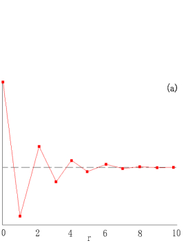
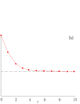
In the large-N๐‘N limit, spin correlations are obtained from Eq.(3.28), see Fig.3.

Refer to caption
Refer to caption
Figure 3: (a)Correlation of ฮ“aโ€‹bsuperscriptฮ“๐‘Ž๐‘\Gamma^{ab} (b)Correlation of ฮ“asuperscriptฮ“๐‘Ž\Gamma^{a}.

III.2.2 Weak-coupling region

We shall consider the weak coupling region g<gc๐‘”subscript๐‘”๐‘g<g_{c}, in which the condensation of zโ€‹(r)๐‘ง๐‘Ÿz(r) occurs. We assume a smooth second-order phase transition from the phase of ฯ‰=0๐œ”0\omega=0 to that of ฯ‰โ‰ 0๐œ”0\omega\neq 0 as ฮณ๐›พ\gamma is increased, and estimate the critical coupling ฮณcsubscript๐›พ๐‘\gamma_{c}fnb . From Eq.(3.28), we divide z๐‘งz as z=z0+z~๐‘งsubscript๐‘ง0~๐‘งz=z_{0}+\tilde{z}, where z0=(z1,0,โ‹ฏ,0,zN)subscript๐‘ง0subscript๐‘ง10โ‹ฏ0subscript๐‘ง๐‘z_{0}=(z_{1},0,\cdots,0,z_{N}), z~=(0,z2,โ‹ฏ,zNโˆ’1,0)~๐‘ง0subscript๐‘ง2โ‹ฏsubscript๐‘ง๐‘10\tilde{z}=(0,z_{2},\cdots,z_{N-1},0). Furthermore we put โŸจฯƒโŸฉ=0delimited-โŸจโŸฉ๐œŽ0\langle\sigma\rangle=0. Substituting the above expression of z๐‘งz into the action, we obtain

S๐‘†\displaystyle S =N2โ€‹gโˆซd3r[zยฏ(โˆ’โˆ‚ฮผ2+ฮปฮผ2+ฮณ|ฯ‰ฮผ|2+ฯƒ)z\displaystyle=\frac{N}{2g}\int d^{3}r\Big{[}\bar{z}(-\partial_{\mu}^{2}+\lambda_{\mu}^{2}+\gamma|\omega_{\mu}|^{2}+\sigma)z
+iฮปฮผzยฏโˆ‚โ†”ฮผzโˆ’ฯ‰ยฏฮผz๐’ฅโˆ‚ฮผzโˆ’ฯ‰ฮผzยฏ๐’ฅโˆ‚ฮผzยฏโˆ’ฯƒ]\displaystyle+i\lambda_{\mu}\bar{z}\overleftrightarrow{\partial}_{\mu}z-\bar{\omega}_{\mu}z\mathcal{J}\partial_{\mu}z-\omega_{\mu}\bar{z}\mathcal{J}\partial_{\mu}\bar{z}-\sigma\Big{]}
=S~+S0,absent~๐‘†subscript๐‘†0\displaystyle=\tilde{S}+S_{0}, (3.34)

where

S~~๐‘†\displaystyle\tilde{S} =N2โ€‹gโˆซd3r[z~ยฏ(โˆ’โˆ‚ฮผ2+ฮปฮผ2+ฮณ|ฯ‰ฮผ|2+ฯƒ)z~\displaystyle=\frac{N}{2g}\int d^{3}r\Big{[}\bar{\tilde{z}}(-\partial_{\mu}^{2}+\lambda_{\mu}^{2}+\gamma|\omega_{\mu}|^{2}+\sigma)\tilde{z}
+iฮปฮผz~ยฏโˆ‚โ†”ฮผz~โˆ’ฯ‰ยฏฮผz~๐’ฅโˆ‚ฮผz~โˆ’ฯ‰ฮผz~ยฏ๐’ฅโˆ‚ฮผz~ยฏโˆ’ฯƒ]\displaystyle+i\lambda_{\mu}\bar{\tilde{z}}\overleftrightarrow{\partial}_{\mu}\tilde{z}-\bar{\omega}_{\mu}\tilde{z}\mathcal{J}\partial_{\mu}\tilde{z}-\omega_{\mu}\bar{\tilde{z}}\mathcal{J}\partial_{\mu}\bar{\tilde{z}}-\sigma\Big{]} (3.35)
S0subscript๐‘†0\displaystyle S_{0} =N2โ€‹gโˆซd3r[zยฏ0(โˆ’โˆ‚ฮผ2+ฮปฮผ2+ฮณ|ฯ‰ฮผ|2+ฯƒ)z0\displaystyle=\frac{N}{2g}\int d^{3}r\Big{[}\bar{z}_{0}(-\partial_{\mu}^{2}+\lambda_{\mu}^{2}+\gamma|\omega_{\mu}|^{2}+\sigma)z_{0}
+iฮปฮผzยฏ0โˆ‚โ†”ฮผz0โˆ’ฯ‰ยฏฮผz0๐’ฅโˆ‚ฮผz0โˆ’ฯ‰ฮผzยฏ0๐’ฅโˆ‚ฮผzยฏ0].\displaystyle+i\lambda_{\mu}\bar{z}_{0}\overleftrightarrow{\partial}_{\mu}z_{0}-\bar{\omega}_{\mu}z_{0}\mathcal{J}\partial_{\mu}z_{0}-\omega_{\mu}\bar{z}_{0}\mathcal{J}\partial_{\mu}\bar{z}_{0}\Big{]}. (3.36)

Integration over z~xsubscript~๐‘ง๐‘ฅ\tilde{z}_{x} can be performed as in the previous case,

โˆซ๐’Ÿโ€‹z~ยฏโ€‹๐’Ÿโ€‹z~โ€‹expโก(โˆ’S~)๐’Ÿยฏ~๐‘ง๐’Ÿ~๐‘ง~๐‘†\displaystyle\int\mathcal{D}\bar{\tilde{z}}\mathcal{D}\tilde{z}\exp(-\tilde{S})
=exp[โˆ’Nโˆ’42โˆซd3r{(โˆ’โˆ‚ฮผ2+ฮปฮผ2+ฮณ|ฯ‰ฮผ|2+ฯƒ)2\displaystyle\hskip 14.22636pt=\exp\Big{[}-\frac{N-4}{2}\int d^{3}r\Big{\{}(-\partial^{2}_{\mu}+\lambda^{2}_{\mu}+\gamma|\omega_{\mu}|^{2}+\sigma)^{2}
+(ฮปฮผโˆ‚โ†”ฮผ)2+ฮณ2|ฯ‰ฮผโˆ‚ฮผ|2}+N2โ€‹gโˆซd3rฯƒ].\displaystyle\hskip 28.45274pt+(\lambda_{\mu}\overleftrightarrow{\partial}_{\mu})^{2}+\gamma^{2}|\omega_{\mu}\partial_{\mu}|^{2}\Big{\}}+{N\over 2g}\int d^{3}r\;\sigma\Big{]}. (3.37)

For S0subscript๐‘†0S_{0}, we substitute the following expression for z0subscript๐‘ง0z_{0},

z0subscript๐‘ง0\displaystyle z_{0} =N0+zโ€ฒ,N0=(12โ€‹n0,0,โ‹ฏ,0,12โ€‹n0),formulae-sequenceabsentsubscript๐‘0superscript๐‘งโ€ฒsubscript๐‘012subscript๐‘›00โ‹ฏ012subscript๐‘›0\displaystyle=N_{0}+z^{\prime},\;N_{0}=(\frac{1}{\sqrt{2}}n_{0},0,\cdots,0,\frac{1}{\sqrt{2}}n_{0}),
zโ€ฒsuperscript๐‘งโ€ฒ\displaystyle z^{\prime} =(z1,0,โ‹ฏ,0,zN),absentsubscript๐‘ง10โ‹ฏ0subscript๐‘ง๐‘\displaystyle=(z_{1},0,\cdots,0,z_{N}), (3.38)

and obtain

S0subscript๐‘†0\displaystyle S_{0} =N2โ€‹gโˆซd3r[zยฏโ€ฒ(โˆ’โˆ‚ฮผ2+ฮปฮผ2+ฮณ|ฯ‰ฮผ|2+ฯƒ)zโ€ฒ\displaystyle=\frac{N}{2g}\int d^{3}r\Big{[}\bar{z}^{\prime}(-\partial_{\mu}^{2}+\lambda_{\mu}^{2}+\gamma|\omega_{\mu}|^{2}+\sigma)z^{\prime}
+iฮปฮผzยฏโ€ฒโˆ‚โ†”ฮผzโ€ฒโˆ’ฯ‰ยฏฮผzโ€ฒ๐’ฅโˆ‚ฮผzโ€ฒโˆ’ฯ‰ฮผzยฏโ€ฒ๐’ฅโˆ‚ฮผzยฏโ€ฒ]\displaystyle+i\lambda_{\mu}\bar{z}^{\prime}\overleftrightarrow{\partial}_{\mu}z^{\prime}-\bar{\omega}_{\mu}z^{\prime}\mathcal{J}\partial_{\mu}z^{\prime}-\omega_{\mu}\bar{z}^{\prime}\mathcal{J}\partial_{\mu}\bar{z}^{\prime}\Big{]}
+Sint,subscript๐‘†int\displaystyle+S_{\mathrm{int}}, (3.39)

where

Sintsubscript๐‘†int\displaystyle S_{\mathrm{int}} =N2โ€‹gโˆซd3r[(ฮปฮผ2+ฮณ|ฯ‰ฮผ|2+ฯƒ){N02+N0(zยฏโ€ฒ+zโ€ฒ)}\displaystyle=\frac{N}{2g}\int d^{3}r\Big{[}(\lambda_{\mu}^{2}+\gamma|\omega_{\mu}|^{2}+\sigma)\{N_{0}^{2}+N_{0}(\bar{z}^{\prime}+z^{\prime})\}
+iฮปฮผN0โˆ‚ฮผ(zโ€ฒโˆ’zยฏโ€ฒ)โˆ’ฮณฯ‰ยฏฮผN0๐’ฅโˆ‚ฮผzโ€ฒโˆ’ฮณฯ‰ฮผN0๐’ฅโˆ‚ฮผzยฏโ€ฒ].\displaystyle+i\lambda_{\mu}N_{0}\partial_{\mu}(z^{\prime}-\bar{z}^{\prime})-\gamma\bar{\omega}_{\mu}N_{0}\mathcal{J}\partial_{\mu}z^{\prime}-\gamma\omega_{\mu}N_{0}\mathcal{J}\partial_{\mu}\bar{z}^{\prime}\Big{]}. (3.40)

We cannot integrate out zโ€ฒsuperscript๐‘งโ€ฒz^{\prime} exactly and therefore treat the cubic terms in Sintsubscript๐‘†intS_{\mathrm{int}} as a โ€œperturbationโ€ of the 1/N1๐‘1/N-expansionan . Then the final expression of the effective action Seffโ€ฒโ€‹(ฮปฮผ,ฯ‰ฮผ)subscriptsuperscript๐‘†โ€ฒeffsubscript๐œ†๐œ‡subscript๐œ”๐œ‡S^{\prime}_{\rm eff}(\lambda_{\mu},\omega_{\mu}) is given as follows up the quadratic terms of ฮปฮผ,ฯƒsubscript๐œ†๐œ‡๐œŽ\lambda_{\mu},\;\sigma and ฯ‰ฮผsubscript๐œ”๐œ‡\omega_{\mu},

Seffโ€ฒโ€‹(ฮปฮผ,ฯ‰ฮผ)subscriptsuperscript๐‘†โ€ฒeffsubscript๐œ†๐œ‡subscript๐œ”๐œ‡\displaystyle S^{\prime}_{\rm eff}(\lambda_{\mu},\omega_{\mu}) =Nโ€‹ฮปฮผโ€‹{ฮ ฮผโ€‹ฮฝ+n02โ€‹(ฮดฮผโ€‹ฮฝโˆ’pฮผโ€‹pฮฝp2)}โ€‹ฮปฮผabsent๐‘subscript๐œ†๐œ‡subscriptฮ ๐œ‡๐œˆsuperscriptsubscript๐‘›02subscript๐›ฟ๐œ‡๐œˆsubscript๐‘๐œ‡subscript๐‘๐œˆsuperscript๐‘2subscript๐œ†๐œ‡\displaystyle={N}\lambda_{\mu}\left\{\Pi_{\mu\nu}+n_{0}^{2}\left(\delta_{\mu\nu}-\frac{p_{\mu}p_{\nu}}{p^{2}}\right)\right\}\lambda_{\mu}
+Nโ€‹ฮณ2โ€‹ฯ‰ฮผRโ€‹{ฮ ฮผโ€‹ฮฝ+n02โ€‹(1ฮณโ€‹ฮดฮผโ€‹ฮฝโˆ’pฮผโ€‹pฮฝp2)+1โˆ’ฮณฮณโ€‹ฮฉฮผโ€‹ฮฝ(1)}โ€‹ฯ‰ฮผR๐‘superscript๐›พ2superscriptsubscript๐œ”๐œ‡๐‘…subscriptฮ ๐œ‡๐œˆsuperscriptsubscript๐‘›021๐›พsubscript๐›ฟ๐œ‡๐œˆsubscript๐‘๐œ‡subscript๐‘๐œˆsuperscript๐‘21๐›พ๐›พsuperscriptsubscriptฮฉ๐œ‡๐œˆ1superscriptsubscript๐œ”๐œ‡๐‘…\displaystyle+{N}\gamma^{2}\omega_{\mu}^{R}\Big{\{}\Pi_{\mu\nu}+n_{0}^{2}\Big{(}\frac{1}{\gamma}\delta_{\mu\nu}-\frac{p_{\mu}p_{\nu}}{p^{2}}\Big{)}+\frac{1-\gamma}{\gamma}\Omega_{\mu\nu}^{(1)}\Big{\}}\omega_{\mu}^{R}
+Nโ€‹ฮณ2โ€‹ฯ‰ฮผIโ€‹{ฮ ฮผโ€‹ฮฝ+n02โ€‹(1ฮณโ€‹ฮดฮผโ€‹ฮฝโˆ’pฮผโ€‹pฮฝp2)+1โˆ’ฮณฮณโ€‹ฮฉฮผโ€‹ฮฝ(1)}โ€‹ฯ‰ฮผI๐‘superscript๐›พ2superscriptsubscript๐œ”๐œ‡๐ผsubscriptฮ ๐œ‡๐œˆsuperscriptsubscript๐‘›021๐›พsubscript๐›ฟ๐œ‡๐œˆsubscript๐‘๐œ‡subscript๐‘๐œˆsuperscript๐‘21๐›พ๐›พsuperscriptsubscriptฮฉ๐œ‡๐œˆ1superscriptsubscript๐œ”๐œ‡๐ผ\displaystyle+{N}\gamma^{2}\omega_{\mu}^{I}\left\{\Pi_{\mu\nu}+n_{0}^{2}\left(\frac{1}{\gamma}\delta_{\mu\nu}-\frac{p_{\mu}p_{\nu}}{p^{2}}\right)+\frac{1-\gamma}{\gamma}\Omega_{\mu\nu}^{(1)}\right\}\omega_{\mu}^{I}
+Nโ€‹ฯƒโ€‹(12โ€‹ฮฃโ€‹(p)+n02)โ€‹ฯƒโˆ’N2โ€‹gโ€‹ฯƒ,๐‘๐œŽ12ฮฃ๐‘subscriptsuperscript๐‘›20๐œŽ๐‘2๐‘”๐œŽ\displaystyle+{N}\sigma\left(\frac{1}{2}\Sigma(p)+n^{2}_{0}\right)\sigma-\frac{N}{2g}\;\sigma, (3.41)

where ฯ‰ฮผ=ฯ‰ฮผR+iโ€‹ฯ‰ฮผIsubscript๐œ”๐œ‡superscriptsubscript๐œ”๐œ‡๐‘…๐‘–superscriptsubscript๐œ”๐œ‡๐ผ\omega_{\mu}=\omega_{\mu}^{R}+i\omega_{\mu}^{I}.

It is obvious that for n0โ‰ 0subscript๐‘›00n_{0}\neq 0 case, only the transverse modes of ฯ‰ฮผsubscript๐œ”๐œ‡\omega_{\mu} (i.e., โˆ‘ฮผpฮผโ€‹ฯ‰ฮผ=0subscript๐œ‡subscript๐‘๐œ‡subscript๐œ”๐œ‡0\sum_{\mu}p_{\mu}\omega_{\mu}=0) can survive at low momentum. Furthermore its mass is renormalized by n0โ‰ 0subscript๐‘›00n_{0}\neq 0 as ฮณโ€‹[n02+(1โˆ’ฮณ)โ€‹ฮฉ(1)]๐›พdelimited-[]subscriptsuperscript๐‘›201๐›พsuperscriptฮฉ1\gamma[n^{2}_{0}+(1-\gamma)\Omega^{(1)}]. Then for ฮณ>ฮณc=1+n02โ€‹(g)ฮฉ(1)๐›พsubscript๐›พ๐‘1subscriptsuperscript๐‘›20๐‘”superscriptฮฉ1\gamma>\gamma_{c}=1+{n^{2}_{0}(g)\over\Omega^{(1)}}, ฮพโ€‹(r)๐œ‰๐‘Ÿ\xi(r), instead of zโ€‹(r)๐‘ง๐‘Ÿz(r), condenses and nontrivial correlations of the โ€œspin operatorsโ€, ฮ“^aโ€‹bsuperscript^ฮ“๐‘Ž๐‘\hat{\Gamma}^{ab}, appear as a result of โŸจฯ‰ฮผโŸฉโ‰ 0delimited-โŸจโŸฉsubscript๐œ”๐œ‡0\langle\omega_{\mu}\rangle\neq 0. In this phase,

โŸจฮ“^aโ€‹bโ€‹(r)โŸฉdelimited-โŸจโŸฉsuperscript^ฮ“๐‘Ž๐‘๐‘Ÿ\displaystyle\langle\hat{\Gamma}^{ab}(r)\rangle =\displaystyle= โŸจzยฏโ€‹(r)โ€‹ฮ“aโ€‹bโ€‹zโ€‹(r)โŸฉdelimited-โŸจโŸฉยฏ๐‘ง๐‘Ÿsuperscriptฮ“๐‘Ž๐‘๐‘ง๐‘Ÿ\displaystyle\langle\bar{z}(r)\Gamma^{ab}z(r)\rangle (3.42)
=\displaystyle= n1aโ€‹bโ€‹cosโก(2โ€‹ฮณโ€‹ฯ‰โ€‹x)+n2aโ€‹bโ€‹sinโก(2โ€‹ฮณโ€‹ฯ‰โ€‹x),superscriptsubscript๐‘›1๐‘Ž๐‘2๐›พ๐œ”๐‘ฅsuperscriptsubscript๐‘›2๐‘Ž๐‘2๐›พ๐œ”๐‘ฅ\displaystyle n_{1}^{ab}\cos(2\gamma\omega x)+n_{2}^{ab}\sin(2\gamma\omega x),

where n1aโ€‹b=Reโ€‹[โŸจฮพโŸฉโ€‹๐’ฅโ€‹ฮ“aโ€‹bโ€‹โŸจฮพโŸฉ],n2aโ€‹b=Imโ€‹[โŸจฮพโŸฉโ€‹๐’ฅโ€‹ฮ“aโ€‹bโ€‹โŸจฮพโŸฉ]formulae-sequencesuperscriptsubscript๐‘›1๐‘Ž๐‘Redelimited-[]delimited-โŸจโŸฉ๐œ‰๐’ฅsuperscriptฮ“๐‘Ž๐‘delimited-โŸจโŸฉ๐œ‰superscriptsubscript๐‘›2๐‘Ž๐‘Imdelimited-[]delimited-โŸจโŸฉ๐œ‰๐’ฅsuperscriptฮ“๐‘Ž๐‘delimited-โŸจโŸฉ๐œ‰n_{1}^{ab}=\mbox{Re}[\langle\xi\rangle\mathcal{J}\Gamma^{ab}\langle\xi\rangle],\;n_{2}^{ab}=\mbox{Im}[\langle\xi\rangle\mathcal{J}\Gamma^{ab}\langle\xi\rangle]. On the other hand, โŸจฮ“^aโ€‹(r)โŸฉ=โŸจฮพยฏโŸฉโ€‹ฮ“aโ€‹โŸจฮพโŸฉdelimited-โŸจโŸฉsuperscript^ฮ“๐‘Ž๐‘Ÿdelimited-โŸจโŸฉยฏ๐œ‰superscriptฮ“๐‘Ždelimited-โŸจโŸฉ๐œ‰\langle\hat{\Gamma}^{a}(r)\rangle=\langle\bar{\xi}\rangle\Gamma^{a}\langle\xi\rangle.

IV SU(2) gauge theory at ฮณ=1๐›พ1\gamma=1

In the previous section, we found that the composite vector field ฯ‰ฮผsubscript๐œ”๐œ‡\omega_{\mu} behaves like a massless gauge field at ฮณ=1๐›พ1\gamma=1, and for g<gc๐‘”subscript๐‘”๐‘g<g_{c} it acquires mass squared propotional to n02=โŸจzยฏโ‹…zโŸฉsuperscriptsubscript๐‘›02delimited-โŸจโŸฉโ‹…ยฏ๐‘ง๐‘งn_{0}^{2}=\langle\bar{z}\cdot z\rangle as a result of the Higgs mechanism. In this section, we shall explicitly show that the three real vector fields (ฮปฮผ,ฯ‰ฮผR,ฯ‰ฮผI)subscript๐œ†๐œ‡subscriptsuperscript๐œ”๐‘…๐œ‡subscriptsuperscript๐œ”๐ผ๐œ‡(\lambda_{\mu},\omega^{R}_{\mu},\omega^{I}_{\mu}) form a SU(2) gauge field minimally coupled with zxsubscript๐‘ง๐‘ฅz_{x} at ฮณ=1๐›พ1\gamma=1. This is another example of the symmetry-enhancement phenomenon, i.e., emergent symmetry at low energies.

We start with the action Sฮณ=1subscript๐‘†๐›พ1S_{\gamma=1} in Eq.(3.12),

Sฮณ=1subscript๐‘†๐›พ1\displaystyle S_{\gamma=1} =N2โ€‹gโ€‹โˆซd3โ€‹rโ€‹[zยฏโ€‹(โˆ’โˆ‚ฮผ2+iโ€‹ฮปฮผโ€‹โˆ‚โ†”ฮผ+ฮปฮผ2+|ฯ‰ฮผ|2+ฯƒ)โ€‹zโˆ’zโ€‹(ฯ‰ยฏฮผโ€‹๐’ฅโ€‹โˆ‚ฮผ)โ€‹zโˆ’zยฏโ€‹(ฯ‰ฮผโ€‹๐’ฅโ€‹โˆ‚ฮผ)โ€‹zยฏโˆ’ฯƒ],absent๐‘2๐‘”superscript๐‘‘3๐‘Ÿdelimited-[]ยฏ๐‘งsuperscriptsubscript๐œ‡2๐‘–subscript๐œ†๐œ‡subscriptโ†”๐œ‡superscriptsubscript๐œ†๐œ‡2superscriptsubscript๐œ”๐œ‡2๐œŽ๐‘ง๐‘งsubscriptยฏ๐œ”๐œ‡๐’ฅsubscript๐œ‡๐‘งยฏ๐‘งsubscript๐œ”๐œ‡๐’ฅsubscript๐œ‡ยฏ๐‘ง๐œŽ\displaystyle=\frac{N}{2g}\int d^{3}r\Big{[}\bar{z}(-\partial_{\mu}^{2}+i\lambda_{\mu}\overleftrightarrow{\partial}_{\mu}+\lambda_{\mu}^{2}+|\omega_{\mu}|^{2}+\sigma)z-z(\bar{\omega}_{\mu}\mathcal{J}\partial_{\mu})z-\bar{z}(\omega_{\mu}\mathcal{J}\partial_{\mu})\bar{z}-\sigma\Big{]}, (4.1)

where we have put ฮณ=1๐›พ1\gamma=1. Hereafter we explicitly consider the CP3 case but generalization to an arbitrary N๐‘N is straightforward. We first redefine the CP3 field Zโ€‹(r)๐‘๐‘ŸZ(r) from the original zโ€‹(r)๐‘ง๐‘Ÿz(r) as follows, Zโ€‹(r)=(z1โ€‹(r),z2โ€‹(r),zยฏ4โ€‹(r),โˆ’zยฏ3โ€‹(r))t๐‘๐‘Ÿsuperscriptsubscript๐‘ง1๐‘Ÿsubscript๐‘ง2๐‘Ÿsubscriptยฏ๐‘ง4๐‘Ÿsubscriptยฏ๐‘ง3๐‘Ÿ๐‘กZ(r)=(z_{1}(r),z_{2}(r),\bar{z}_{4}(r),-\bar{z}_{3}(r))^{t}. It is easily verified that Zโ€‹(r)๐‘๐‘ŸZ(r) is a CP3 field, โˆ‘i=14|Ziโ€‹(r)|2=1.subscriptsuperscript4๐‘–1superscriptsubscript๐‘๐‘–๐‘Ÿ21\sum^{4}_{i=1}|Z_{i}(r)|^{2}=1.

It is straightfward to verify the following equation,

zยฏโ€‹โˆ‚โ†”ฮผโ€‹z=Zยฏโ€‹ฮฃ3โ€‹โˆ‚โ†”ฮผโ€‹Z,ยฏ๐‘งsubscriptโ†”๐œ‡๐‘งยฏ๐‘subscriptฮฃ3subscriptโ†”๐œ‡๐‘\bar{z}\overleftrightarrow{\partial}_{\mu}z=\bar{Z}\Sigma_{3}\overleftrightarrow{\partial}_{\mu}Z, (4.2)

where

ฮฃ3=(1000010000โˆ’10000โˆ’1).subscriptฮฃ31000010000100001\Sigma_{3}=\left(\begin{array}[]{cccc}1&0&0&0\\ 0&1&0&0\\ 0&0&-1&0\\ 0&0&0&-1\end{array}\right). (4.3)

Similarly

ฯ‰ยฏฮผโ€‹(zโ€‹๐’ฅโ€‹โˆ‚ฮผ)โ€‹z+ฯ‰ฮผโ€‹(zยฏโ€‹๐’ฅโ€‹โˆ‚ฮผ)โ€‹zยฏ=iโ€‹ฯ‰ฮผRโ€‹(Zยฏโ€‹ฮฃ2โ€‹โˆ‚โ†”ฮผโ€‹Z)+iโ€‹ฯ‰ฮผIโ€‹(Zยฏโ€‹ฮฃ1โ€‹โˆ‚โ†”ฮผโ€‹Z),subscriptยฏ๐œ”๐œ‡๐‘ง๐’ฅsubscript๐œ‡๐‘งsubscript๐œ”๐œ‡ยฏ๐‘ง๐’ฅsubscript๐œ‡ยฏ๐‘ง๐‘–subscriptsuperscript๐œ”๐‘…๐œ‡ยฏ๐‘subscriptฮฃ2subscriptโ†”๐œ‡๐‘๐‘–subscriptsuperscript๐œ”๐ผ๐œ‡ยฏ๐‘subscriptฮฃ1subscriptโ†”๐œ‡๐‘\displaystyle\bar{\omega}_{\mu}(z\mathcal{J}\partial_{\mu})z+\omega_{\mu}(\bar{z}\mathcal{J}\partial_{\mu})\bar{z}=i\omega^{R}_{\mu}(\bar{Z}\Sigma_{2}\overleftrightarrow{\partial}_{\mu}Z)+i\omega^{I}_{\mu}(\bar{Z}\Sigma_{1}\overleftrightarrow{\partial}_{\mu}Z), (4.4)

where

๐’ฅ=(000100โˆ’100100โˆ’1000),ฮฃ2=(00i0000iโˆ’i0000โˆ’i00),formulae-sequence๐’ฅ0001001001001000subscriptฮฃ200๐‘–0000๐‘–๐‘–0000๐‘–00\mathcal{J}=\left(\begin{array}[]{cccc}0&0&0&1\\ 0&0&-1&0\\ 0&1&0&0\\ -1&0&0&0\end{array}\right),\;\;\Sigma_{2}=\left(\begin{array}[]{cccc}0&0&i&0\\ 0&0&0&i\\ -i&0&0&0\\ 0&-i&0&0\end{array}\right),
ฮฃ1=(0010000110000100).subscriptฮฃ10010000110000100\Sigma_{1}=\left(\begin{array}[]{cccc}0&0&1&0\\ 0&0&0&1\\ 1&0&0&0\\ 0&1&0&0\end{array}\right). (4.5)

It is obvious that ฮฃiโ€‹(i=1,2,3)subscriptฮฃ๐‘–๐‘–123\Sigma_{i}(i=1,2,3) satisfy the SU(2) algebra. Let us define SU(2) gauge field ๐’œโ†’ฮผsubscriptโ†’๐’œ๐œ‡\vec{\cal A}_{\mu} as ๐’œโ†’ฮผ=(ฮปฮผ1,ฮปฮผ2,ฮปฮผ3)=(ฯ‰ฮผI,ฯ‰ฮผR,ฮปฮผ)subscriptโ†’๐’œ๐œ‡subscriptsuperscript๐œ†1๐œ‡subscriptsuperscript๐œ†2๐œ‡subscriptsuperscript๐œ†3๐œ‡subscriptsuperscript๐œ”๐ผ๐œ‡subscriptsuperscript๐œ”๐‘…๐œ‡subscript๐œ†๐œ‡\vec{\cal A}_{\mu}=(\lambda^{1}_{\mu},\lambda^{2}_{\mu},\lambda^{3}_{\mu})=(\omega^{I}_{\mu},\omega^{R}_{\mu},\lambda_{\mu}), then the Lagrangian (4.1) can be rewritten as follows,

Sฮณ=1=N2โ€‹gโ€‹โˆซd3โ€‹rโ€‹[|(โˆ‚ฮผ+iโ€‹ฮฃโ†’โ‹…๐’œโ†’ฮผ)โ€‹Z|2+ฯƒโ€‹|Z|2โˆ’ฯƒ].subscript๐‘†๐›พ1๐‘2๐‘”superscript๐‘‘3๐‘Ÿdelimited-[]superscriptsubscript๐œ‡โ‹…๐‘–โ†’ฮฃsubscriptโ†’๐’œ๐œ‡๐‘2๐œŽsuperscript๐‘2๐œŽS_{\gamma=1}=\frac{N}{2g}\int d^{3}r\Big{[}|(\partial_{\mu}+i\vec{\Sigma}\cdot\vec{\cal A}_{\mu})Z|^{2}+\sigma|Z|^{2}-\sigma\Big{]}. (4.6)

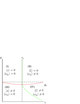
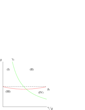
Lattice gauge model corresponding to the above SU(2) gauge theory (4.6) is under study and result will be reported in a future publication. However phase structure of the system can be inferred by qualitative discussion. As in the usual CPN-1 model coupled with the U(1) gauge field, there exists a phase transition that separates ordered and disordered phases. However, as the SU(2) gauge field fluctuates the hopping of the spinon Zโ€‹(r)๐‘๐‘ŸZ(r) more strongly than the U(1) gauge field, the critical coupling gcโ€‹(ฮณ=1)subscript๐‘”๐‘๐›พ1g_{c}(\gamma=1) is expected to be smaller than gcโ€‹(ฮณ=0)subscript๐‘”๐‘๐›พ0g_{c}(\gamma=0). From this consideration, we expect that the critical coupling gcโ€‹(ฮณ)subscript๐‘”๐‘๐›พg_{c}(\gamma) is a decreasing function of ฮณ๐›พ\gamma for ฮณ<ฮณc๐›พsubscript๐›พ๐‘\gamma<\gamma_{c}, though in the previous discussion for small ฮณโ‰ช1much-less-than๐›พ1\gamma\ll 1 by the 1/N1๐‘1/N-expansion we do not find any ฮณ๐›พ\gamma dependence of gcsubscript๐‘”๐‘g_{c}. As ฮณ๐›พ\gamma exceeds ฮณcsubscript๐›พ๐‘\gamma_{c}, the condensation of ฯ‰ฮผsubscript๐œ”๐œ‡\omega_{\mu} tends to occur and fluctuations of ฯ‰ฮผsubscript๐œ”๐œ‡\omega_{\mu} are suppressed. Moreover the original U(1) gauge symmetry reduces to Z2subscript๐‘2Z_{2} gauge symmetry by the Anderson-Higgs mechanism and fluctuations of ฮปฮผsubscript๐œ†๐œ‡\lambda_{\mu} are also suppressed. Then gcโ€‹(ฮณ)subscript๐‘”๐‘๐›พg_{c}(\gamma) starts to increase at ฮณ=ฮณc๐›พsubscript๐›พ๐‘\gamma=\gamma_{c}. The above expectation will be confirmed by the numerical study of lattice-gauge model in the following section. Expected phase diagram is show in the (ฮณโˆ’g)โˆ’limit-from๐›พ๐‘”(\gamma-g)- plane in Fig.4.

Refer to caption
Refer to caption
Figure 4: Phase diagram in (ฮณโˆ’g)๐›พ๐‘”(\gamma-g) and (ฮณ/gโˆ’g)โˆ’limit-from๐›พ๐‘”๐‘”(\gamma/g-g)- planes.

In the following section, we shall introduce a lattice model for the effective field theory with general value of ฮณ๐›พ\gamma, and study it by means of MC simulations.
Refer to caption
Figure 5: Interaction terms in ALsubscript๐ด๐ฟA_{L} in Eq.(5.1).
Refer to caption
Refer to caption
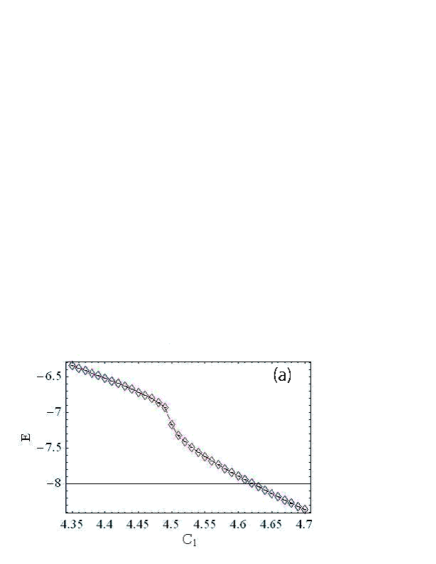
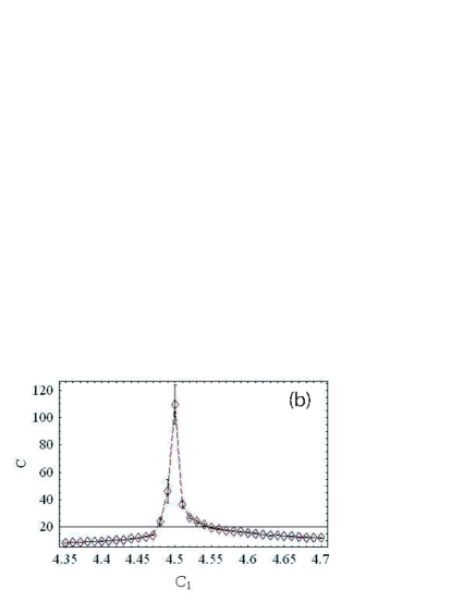
Figure 6: (a)Enegry E๐ธE as a function of c1subscript๐‘1c_{1} for c2=c3=0subscript๐‘2subscript๐‘30c_{2}=c_{3}=0. There exists a discontinuity at c1=4.5subscript๐‘14.5c_{1}=4.5. (b)โ€œSpecific heatโ€ C๐ถC as a function of c1subscript๐‘1c_{1} for c2=c3=0subscript๐‘2subscript๐‘30c_{2}=c_{3}=0. There exists a sharp peak at c1=4.5subscript๐‘14.5c_{1}=4.5. System size L=20๐ฟ20L=20.

V Numerical study

Refer to caption
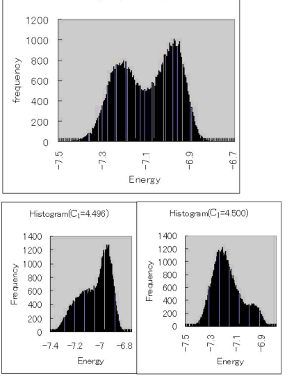
Figure 7: Enegry distribution Nโ€‹[E]๐‘delimited-[]๐ธN[E] for the pure CP3 model. At c1=4.498subscript๐‘14.498c_{1}=4.498, Nโ€‹(E)๐‘๐ธN(E) has double-peak shape, whereas it has single peak at c1=4.496subscript๐‘14.496c_{1}=4.496 and 4.5004.5004.500. System size L=20๐ฟ20L=20.

In this section we formulate the effective field theory (3.1) on a cubic lattice, and investigate its phase structure by means of the MC simulations. We explicitly consider the Sp(4) model. Action of the lattice model ALsubscript๐ด๐ฟA_{L} is given as follows,

ALsubscript๐ด๐ฟ\displaystyle A_{L} =c1โ€‹โˆ‘r,ฮผzยฏr+ฮผโ€‹Urโ€‹ฮผโ€‹zr+c.c.absentsubscript๐‘1subscript๐‘Ÿ๐œ‡subscriptยฏ๐‘ง๐‘Ÿ๐œ‡subscript๐‘ˆ๐‘Ÿ๐œ‡subscript๐‘ง๐‘Ÿc.c.\displaystyle=c_{1}\sum_{r,\mu}\bar{z}_{r+\mu}U_{r\mu}z_{r}+\mbox{c.c.}
+c2โ€‹โˆ‘r,ฮผ,ฮฝUrโ€‹ฮผโ€‹Ur+ฮผ,ฮฝโ€‹Uยฏr+ฮฝ,ฮผโ€‹Uยฏrโ€‹ฮฝ+c.c.subscript๐‘2subscript๐‘Ÿ๐œ‡๐œˆsubscript๐‘ˆ๐‘Ÿ๐œ‡subscript๐‘ˆ๐‘Ÿ๐œ‡๐œˆsubscriptยฏ๐‘ˆ๐‘Ÿ๐œˆ๐œ‡subscriptยฏ๐‘ˆ๐‘Ÿ๐œˆc.c.\displaystyle+c_{2}\sum_{r,\mu,\nu}U_{r\mu}U_{r+\mu,\nu}\bar{U}_{r+\nu,\mu}\bar{U}_{r\nu}+\mbox{c.c.}
+c3โ€‹โˆ‘r,ฮผ|zrโ€‹๐’ฅโ€‹zr+ฮผ|2+c4โ€‹โˆ‘r,ฮผ|zrโ€‹๐’ฅโ€‹zr+1+2|2,subscript๐‘3subscript๐‘Ÿ๐œ‡superscriptsubscript๐‘ง๐‘Ÿ๐’ฅsubscript๐‘ง๐‘Ÿ๐œ‡2subscript๐‘4subscript๐‘Ÿ๐œ‡superscriptsubscript๐‘ง๐‘Ÿ๐’ฅsubscript๐‘ง๐‘Ÿ122\displaystyle+c_{3}\sum_{r,\mu}|z_{r}\mathcal{J}z_{r+\mu}|^{2}+c_{4}\sum_{r,\mu}|z_{r}\mathcal{J}z_{r+1+2}|^{2}, (5.1)

where r๐‘Ÿr denotes the cubic lattice site, ฮผ=(0,1,2)๐œ‡012\mu=(0,1,2) is the direction index and it also denotes the unit vector in the ฮผ๐œ‡\mu-direction. Field zrsubscript๐‘ง๐‘Ÿz_{r}โ€™s are CP3 variables and Urโ€‹ฮผsubscript๐‘ˆ๐‘Ÿ๐œ‡U_{r\mu} is a U(1) gauge field defined on link (r,ฮผ)๐‘Ÿ๐œ‡(r,\mu), Urโ€‹ฮผโˆผeiโ€‹ฮปฮผโ€‹(r)similar-tosubscript๐‘ˆ๐‘Ÿ๐œ‡superscript๐‘’๐‘–subscript๐œ†๐œ‡๐‘ŸU_{r\mu}\sim e^{i\lambda_{\mu}(r)}. The parameters c1โˆ1/gproportional-tosubscript๐‘11๐‘”c_{1}\propto 1/g, c3โˆฮณ/gproportional-tosubscript๐‘3๐›พ๐‘”c_{3}\propto\gamma/g and the c2subscript๐‘2c_{2}-term is the lattice Maxwell term (the so-called Wilson term) corresponding to (โˆ‚ฮผAฮฝโˆ’โˆ‚ฮฝAฮผ)2superscriptsubscript๐œ‡subscript๐ด๐œˆsubscript๐œˆsubscript๐ด๐œ‡2(\partial_{\mu}A_{\nu}-\partial_{\nu}A_{\mu})^{2} in the continuum spacetimefnb . We also added the c4subscript๐‘4c_{4}-term on the diagonal lines in the 2D layers that represents the exchange couplings between spins on even sites of the original lattice. See Fig.5. The partition function ZLsubscript๐‘๐ฟZ_{L} is given as

ZL=โˆซ[Dโ€‹U]โ€‹[Dโ€‹zโ€‹Dโ€‹zยฏ]CPโ€‹eAL,subscript๐‘๐ฟdelimited-[]๐ท๐‘ˆsubscriptdelimited-[]๐ท๐‘ง๐ทยฏ๐‘งCPsuperscript๐‘’subscript๐ด๐ฟZ_{L}=\int[DU][DzD\bar{z}]_{\rm CP}\;e^{A_{L}}, (5.2)

where [Dโ€‹zโ€‹Dโ€‹zยฏ]CPsubscriptdelimited-[]๐ท๐‘ง๐ทยฏ๐‘งCP[DzD\bar{z}]_{\rm CP} denotes the integration over CP3 variables, and we use a specific parameterization for them in the MC simulations. For the MC simulations, we used the standard Metropolis algorithm of local update. The typical statistics was 105superscript10510^{5} MC steps per sample, and the averages and errors were estimated over ten samples. The typical acceptance ratio was about 505050%. We also used multi-histogram methods to obtain reliable results near the phase transition pointmhm .
Refer to caption
Refer to caption
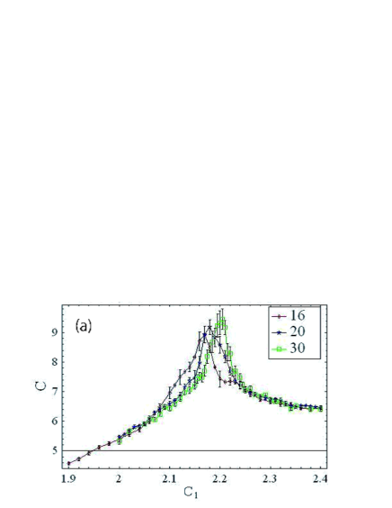
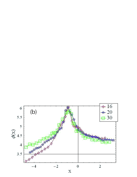
Figure 8: (a)C๐ถC for c2=2.0,c3=0formulae-sequencesubscript๐‘22.0subscript๐‘30c_{2}=2.0,\;c_{3}=0. System size is L=16,โ€„20,โ€„30๐ฟ162030L=16,\;20,\;30. (b)Scaling function ฯ•โ€‹(x)italic-ฯ•๐‘ฅ\phi(x) in finite-size scaling (5.4). Critical exponents and critical coupling are estimated as ฮฝ=0.8,ฯƒ=0.11formulae-sequence๐œˆ0.8๐œŽ0.11\nu=0.8,\;\sigma=0.11 and c1โ€‹c=2.23subscript๐‘1๐‘2.23c_{1c}=2.23.

We first consider the case of the pure CP3 model with c2=c3=c4=0subscript๐‘2subscript๐‘3subscript๐‘40c_{2}=c_{3}=c_{4}=0, which corresponds to the anisotropic SU(4) AF magnetkawashima . We calculate the โ€œinternal energyโ€ E=โŸจALโŸฉ/L3๐ธdelimited-โŸจโŸฉsubscript๐ด๐ฟsuperscript๐ฟ3E=\langle A_{L}\rangle/L^{3} and the โ€œspecific heatโ€ C=โŸจ(ALโˆ’E)2โŸฉ/L3๐ถdelimited-โŸจโŸฉsuperscriptsubscript๐ด๐ฟ๐ธ2superscript๐ฟ3C=\langle(A_{L}-E)^{2}\rangle/L^{3} to study phase structure, where L3superscript๐ฟ3L^{3} is the lattice size and we impose the periodic boundary condition in moose of calculations. In Fig.6, we show E๐ธE and C๐ถC as a function of c1subscript๐‘1c_{1}. It is obvious that E๐ธE has a discontinuity at c1โ‰ƒ4.5similar-to-or-equalssubscript๐‘14.5c_{1}\simeq 4.5 and C๐ถC has a very large peak at c1โ‰ƒ4.5similar-to-or-equalssubscript๐‘14.5c_{1}\simeq 4.5, which indicates a first-order phase transition. In order to verify this observation, we calculated density of states Nโ€‹[E]๐‘delimited-[]๐ธN[E] that is defined as

Nโ€‹[E]=โˆซ[Dโ€‹U]โ€‹[Dโ€‹zโ€‹Dโ€‹zยฏ]CPโ€‹ฮดโ€‹(ALโˆ’E)โ€‹eAL.๐‘delimited-[]๐ธdelimited-[]๐ท๐‘ˆsubscriptdelimited-[]๐ท๐‘ง๐ทยฏ๐‘งCP๐›ฟsubscript๐ด๐ฟ๐ธsuperscript๐‘’subscript๐ด๐ฟN[E]=\int[DU][DzD\bar{z}]_{\rm CP}\;\delta(A_{L}-E)\;e^{A_{L}}. (5.3)

Result in Fig.7 shows that Nโ€‹[E]๐‘delimited-[]๐ธN[E] has a double-peak shape at c1=4.498subscript๐‘14.498c_{1}=4.498, whereas it has a single peak at the other couplings. This confirms the existence of the first-order phase transition in the CP3 model, though corresponding phase transitions in the CP1 and CP2 models are of second order. Study of the correlation functions of the โ€œspinโ€ operators given later on shows that phase transition from โ€œNรฉelโ€ to paramagnetic states takes place at c1=4.498subscript๐‘14.498c_{1}=4.498.

CPN-1 model in the 3D spacetime was studied by the 1/N1๐‘1/N-expansion and it was suggested that there existed a second-order phase transition from ordered to disordered phases as the coupling constant is increased. However the present investigation by means of the MC simulations shows that the order of the phase transition varies as a function of the parameter N๐‘N. Similar phenomenon was recently observed some related model, e.g. multi-Higgs U(1) gauge model in 3D. We also studied finite but small c2subscript๐‘2c_{2} cases and found that the phase transition is still of first-order. However at intermediate value of c2subscript๐‘2c_{2}, C๐ถC exhibits the finite-size scaling (see Fig.8), i.e., the data of Cโ€‹(c1,L)๐ถsubscript๐‘1๐ฟC(c_{1},L) for system size L๐ฟL and c2=2.0subscript๐‘22.0c_{2}=2.0 can be fit as follows with a scaling function ฯ•โ€‹(x)italic-ฯ•๐‘ฅ\phi(x)fss ,

Cโ€‹(c1,L)=Lฯƒ/ฮฝโ€‹ฯ•โ€‹(L1/ฮฝโ€‹ฯต),ฯต=(c1โˆ’c1โ€‹c)/c1โ€‹c,formulae-sequence๐ถsubscript๐‘1๐ฟsuperscript๐ฟ๐œŽ๐œˆitalic-ฯ•superscript๐ฟ1๐œˆitalic-ฯตitalic-ฯตsubscript๐‘1subscript๐‘1๐‘subscript๐‘1๐‘C(c_{1},L)=L^{\sigma/\nu}\phi(L^{1/\nu}\epsilon),\;\;\;\epsilon=(c_{1}-c_{1c})/c_{1c}, (5.4)

where c1โ€‹csubscript๐‘1๐‘c_{1c} is the critical coupling at infinite system size and estimated as c1โ€‹c=2.23subscript๐‘1๐‘2.23c_{1c}=2.23. This fact means that the phase transition becomes of second-order as the value of c2subscript๐‘2c_{2} is increased.

Refer to caption
Refer to caption
Figure 9: (a)C๐ถC for c2=2.0,c3=1.0formulae-sequencesubscript๐‘22.0subscript๐‘31.0c_{2}=2.0,\;c_{3}=1.0. System size is L=14,โ€„20,โ€„30๐ฟ142030L=14,\;20,\;30. Critical coupling is estimated at c1=2.35subscript๐‘12.35c_{1}=2.35. (b)C๐ถC for c1=3.0,c2=2.0formulae-sequencesubscript๐‘13.0subscript๐‘22.0c_{1}=3.0,\;c_{2}=2.0. System size is L=18๐ฟ18L=18. There are two phase transitions at c3=3.7subscript๐‘33.7c_{3}=3.7 and 5.25.25.2.

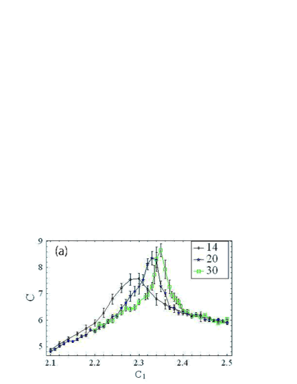
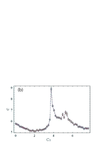
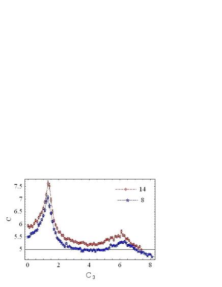
Let us turn on the c3subscript๐‘3c_{3}-term and see how location of the phase transition varies. We studied the system by varying value of c1subscript๐‘1c_{1} with fixed c3subscript๐‘3c_{3}, and found clear signal of phase transitions, see, e.g. C๐ถC for c2=2.0,c3=1.0formulae-sequencesubscript๐‘22.0subscript๐‘31.0c_{2}=2.0,\;c_{3}=1.0 in Fig.9. We also investigated phase structure of the system with c1subscript๐‘1c_{1} fixed and c3subscript๐‘3c_{3} varied, and found that there is another phase transition line. See Fig.9.
Refer to caption
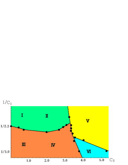
Figure 10: Phase diagram in (c3โˆ’1c1)subscript๐‘31subscript๐‘1(c_{3}-{1\over c_{1}}) plane for c2=2.0subscript๐‘22.0c_{2}=2.0. Solid lines are phase transition lines obtained by measurement of E๐ธE and C๐ถC. Dots denote phase transition points actually observed by measurement. โ€œSpinโ€ correlation functions exhibit different behavior in regions IโˆผVโ€‹Isimilar-to๐ผ๐‘‰๐ผI\sim VI. Similar phase structure is obtained for c2=0subscript๐‘20c_{2}=0.
Refer to caption
Refer to caption
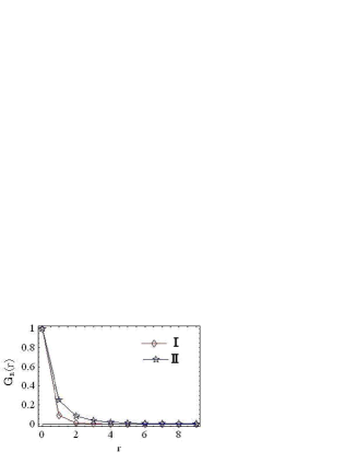
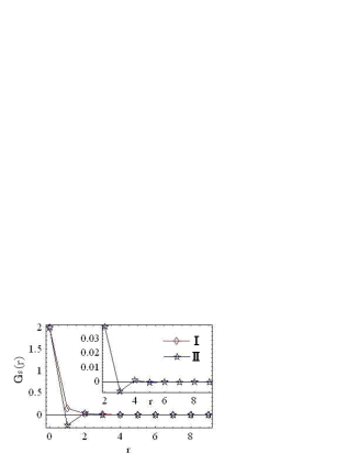
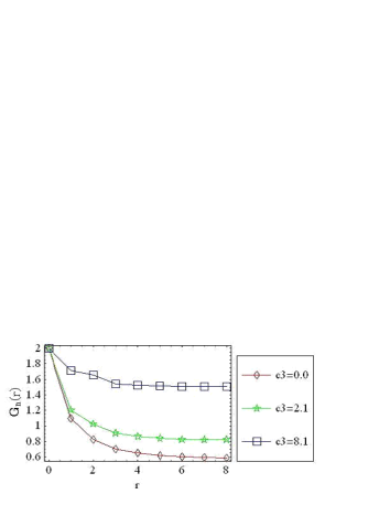
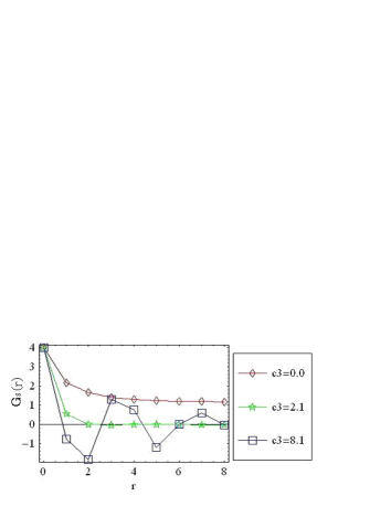
Figure 11: Spin correlation functions in I๐ผI and Iโ€‹I๐ผ๐ผII in phase diagram Fig.10. Both Gnโ€‹(r)subscript๐บ๐‘›๐‘ŸG_{n}(r) and Gsโ€‹(r)subscript๐บ๐‘ ๐‘ŸG_{s}(r) have no long-range order in I๐ผI and Iโ€‹I๐ผ๐ผII, however in Iโ€‹I๐ผ๐ผII Gsโ€‹(r)subscript๐บ๐‘ ๐‘ŸG_{s}(r) exhibits a short-range spiral order.
Refer to caption
Refer to caption
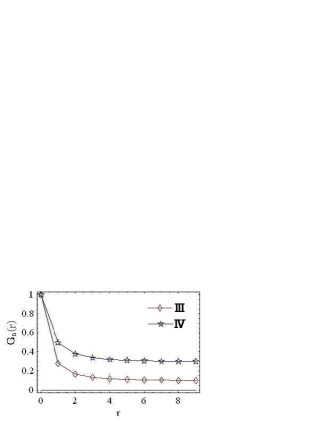
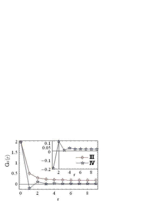
Figure 12: Spin correlation functions in Iโ€‹Iโ€‹I๐ผ๐ผ๐ผIII and Iโ€‹V๐ผ๐‘‰IV in phase diagram Fig.10. Gnโ€‹(r)subscript๐บ๐‘›๐‘ŸG_{n}(r) has long-range order both in Iโ€‹Iโ€‹I๐ผ๐ผ๐ผIII and Iโ€‹V๐ผ๐‘‰IV. In Iโ€‹V๐ผ๐‘‰IV, Gsโ€‹(r)subscript๐บ๐‘ ๐‘ŸG_{s}(r) exhibits a long-range spiral order, whereas it has usual long-range order in Iโ€‹Iโ€‹I๐ผ๐ผ๐ผIII.
Refer to caption
Refer to caption
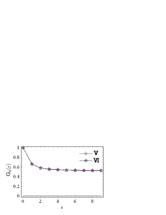
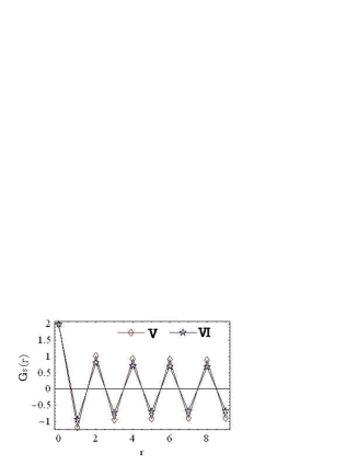
Figure 13: Spin correlation functions in V๐‘‰V and Vโ€‹I๐‘‰๐ผVI in phase diagram Fig.10. Both Gnโ€‹(r)subscript๐บ๐‘›๐‘ŸG_{n}(r) and Gsโ€‹(r)subscript๐บ๐‘ ๐‘ŸG_{s}(r) exhibit the same behavior in V๐‘‰V and Vโ€‹I๐‘‰๐ผVI.
Refer to caption
Figure 14: Specific heat on line c3=c4subscript๐‘3subscript๐‘4c_{3}=c_{4} with c1=6,c2=0formulae-sequencesubscript๐‘16subscript๐‘20c_{1}=6,\;c_{2}=0. Result indicates two phase transitions on the line.
Refer to caption
Refer to caption
Figure 15: Spin correlation functions for c1=6.0subscript๐‘16.0c_{1}=6.0 and c2=0subscript๐‘20c_{2}=0.

Obtained phase diagram in the (c3โˆ’1c1)subscript๐‘31subscript๐‘1(c_{3}-{1\over c_{1}}) plane is shown in Fig.10. There are four phases, which are identified by the measurement of E๐ธE and C๐ถC. We also investigated the behavior of the correlation function of the โ€œspinโ€ operators,

Gnโ€‹(r)=โˆ‘aโŸจฮ“rโ€ฒ+raโ€‹ฮ“rโ€ฒaโŸฉ,Gsโ€‹(r)=โˆ‘aโ€‹bโŸจฮ“rโ€ฒ+raโ€‹bโ€‹ฮ“rโ€ฒaโ€‹bโŸฉ.formulae-sequencesubscript๐บ๐‘›๐‘Ÿsubscript๐‘Ždelimited-โŸจโŸฉsubscriptsuperscriptฮ“๐‘Žsuperscript๐‘Ÿโ€ฒ๐‘Ÿsubscriptsuperscriptฮ“๐‘Žsuperscript๐‘Ÿโ€ฒsubscript๐บ๐‘ ๐‘Ÿsubscript๐‘Ž๐‘delimited-โŸจโŸฉsubscriptsuperscriptฮ“๐‘Ž๐‘superscript๐‘Ÿโ€ฒ๐‘Ÿsubscriptsuperscriptฮ“๐‘Ž๐‘superscript๐‘Ÿโ€ฒG_{n}(r)=\sum_{a}\langle\Gamma^{a}_{r^{\prime}+r}\Gamma^{a}_{r^{\prime}}\rangle,\;\;G_{s}(r)=\sum_{ab}\langle\Gamma^{ab}_{r^{\prime}+r}\Gamma^{ab}_{r^{\prime}}\rangle. (5.5)

As we expect that a phase transition to a โ€œspiral stateโ€ takes place as the parameters are increased, we take the free boundary condition in the two spatial directions. We found that the correlators exhibit different behavior in the six โ€œregionsโ€ IโˆผVโ€‹Isimilar-to๐ผ๐‘‰๐ผI\sim VI shown in Fig.10. It is obvious that not only simple ferromagnetic(FM) correlation, antiferromagnetic(AF) correlations appear in these correlators. For example in the regions I๐ผI and Iโ€‹I๐ผ๐ผII (Iโ€‹Iโ€‹I๐ผ๐ผ๐ผIII and Iโ€‹V๐ผ๐‘‰IV), the correlation of the nematic order Gnโ€‹(r)subscript๐บ๐‘›๐‘ŸG_{n}(r) exhibits the same behavior, but the spin correlator Gsโ€‹(r)subscript๐บ๐‘ ๐‘ŸG_{s}(r) behaves differently in I๐ผI and Iโ€‹I๐ผ๐ผII (Iโ€‹Iโ€‹I๐ผ๐ผ๐ผIII and Iโ€‹V๐ผ๐‘‰IV), see Fig.11 (Fig.12). We have observed no phase boundary between the I๐ผI and Iโ€‹I๐ผ๐ผII (Iโ€‹Iโ€‹I๐ผ๐ผ๐ผIII and Iโ€‹V๐ผ๐‘‰IV) regions on which the internal energy E๐ธE and specific heat C๐ถC exhibit anomalous behavior. However from the result of the spin correlation function, Gsโ€‹(r)subscript๐บ๐‘ ๐‘ŸG_{s}(r), we expect that the phases โŸจฯ‰ฮผโŸฉโ‰ 0,โŸจฮพโ€‹(r)โŸฉ=0formulae-sequencedelimited-โŸจโŸฉsubscript๐œ”๐œ‡0delimited-โŸจโŸฉ๐œ‰๐‘Ÿ0\langle\omega_{\mu}\rangle\neq 0,\;\langle\xi(r)\rangle=0 and โŸจฯ‰ฮผโŸฉโ‰ 0,โŸจฮพโ€‹(r)โŸฉโ‰ 0formulae-sequencedelimited-โŸจโŸฉsubscript๐œ”๐œ‡0delimited-โŸจโŸฉ๐œ‰๐‘Ÿ0\langle\omega_{\mu}\rangle\neq 0,\;\langle\xi(r)\rangle\neq 0 are realized in the regions Iโ€‹I๐ผ๐ผII and Iโ€‹V๐ผ๐‘‰IV, respectively. On the other hand, there are no phases in the effective field theory that correspond to the phases V๐‘‰V and Vโ€‹I๐‘‰๐ผVI of the FM long-range order in the lattice model.

Finally we turn on the c4subscript๐‘4c_{4}-term in addition to the c3subscript๐‘3c_{3}-term. Numerical study of the system was performed along the line c3=c4subscript๐‘3subscript๐‘4c_{3}=c_{4} with c1=6.0subscript๐‘16.0c_{1}=6.0 and c2=0subscript๐‘20c_{2}=0 in the phase diagram. Observed C๐ถC as a function of c3=c4subscript๐‘3subscript๐‘4c_{3}=c_{4} is shown in Fig.14. There are two phase transition, one at c3=c4โ‰ƒ0.7subscript๐‘3subscript๐‘4similar-to-or-equals0.7c_{3}=c_{4}\simeq 0.7 and the other at c3=c4โ‰ƒ6.0subscript๐‘3subscript๐‘4similar-to-or-equals6.0c_{3}=c_{4}\simeq 6.0. In order to understand these phase transitions, we calculated the spin correlation functions in each phase, which are shown in Fig.15. From the result, it is obvious that the AF order disappears first and then at the second transition the spiral state appears. This state corresponds to the state with nonvanishing โŸจฮพโ€‹(r)โŸฉโ‰ 0delimited-โŸจโŸฉ๐œ‰๐‘Ÿ0\langle\xi(r)\rangle\neq 0 studied in the previous sections.

VI Conclusion

In the present paper, we have studied the Sp(N) AF Heisenberg model in 2D that is expected to be realized in cold atom system in an optical lattice. We focus on the ground state structure of the system and derived the effective field theory for the system, which is a kind of extension of the CPN-1 nonlinear ฯƒ๐œŽ\sigma-model. Then we studied the phase structure and critical behavior by using the 1/N1๐‘1/N-expansion. We found that the spatial anisotropy induces a phase transition from the ordered state to paramagnetic state. As the explicit breaking of the SU(N) symmetry increases, the ground state exhibits a spiral order of the ad joint representation of Sp(N) group. This state also has a nematic order of vector representation of the Sp(N) group.

We also introduced a lattice gauge-model counterpart of the effective field theory, and studied its phase structure by means of the MC simulations. We found a similar phase diagram with that of the field theory, but order of the phase transitions is different in two systems.

In Ref.xu , finite-temperature phase diagram of Sp(N) model is studied by using a Ginzburg-Landau theory in terms of gauge-invariant spin fields, ฯ•aโ€‹b=zโ€ โ€‹ฮ“aโ€‹bโ€‹z,ฯ•a=zโ€ โ€‹ฮ“aโ€‹bโ€‹zformulae-sequencesuperscriptitalic-ฯ•๐‘Ž๐‘superscript๐‘งโ€ superscriptฮ“๐‘Ž๐‘๐‘งsuperscriptitalic-ฯ•๐‘Žsuperscript๐‘งโ€ superscriptฮ“๐‘Ž๐‘๐‘ง\phi^{ab}=z^{\dagger}\Gamma^{ab}z,\;\phi^{a}=z^{\dagger}\Gamma^{ab}z. There quantum phase transition of Sp(4) spin system in 3D stacked square lattice is also discussed. Phase transition from CP3 Nรฉel ordered state to photon liquid state is predicted. In the (3+1)D counterpart of the lattice model (5.1), it is expected that deconfined photon phase exists for sufficiently large c2subscript๐‘2c_{2}. U(1) gauge theory of CP1 field in (3+1)D was studied previouslysawamura , and it was found that phase transition from CP1 Nรฉel ordered state to photon liquid state is of second order.

It is interesting to study effects of hole doping to the Sp(N) AF magnets and investigate how the long-range orders are broken and if a new phase with hole-pair condensation appears. This system is an extension of the t-J model for high-temperature superconductivity. This problem is under study and we hope that results will be reported in a future publication.


Acknowledgment

This work was partially supported by Grant-in-Aid for Scientific Research from Japan Society for the Promotion of Science under Grant No.20540264.

Appendix A Derivation of the effective field theory

In Sec.2, we derived the effective field theory of the Sp(N) AF Heisenberg model. In the present appendix, we give some details of the derivation.

In Eq.(2.14), Aโ€‹(ฯ„)๐ด๐œA(\tau) is expanded in powers of ๐ฉ๐ฉ{\bf p} and ๐ฉยฏยฏ๐ฉ\bar{\bf p}. Vectors ๐ค๐ค{\bf k} and ๐ฅยฏยฏ๐ฅ\bar{\bf l} are explicitly given as follows,

๐ค=(โˆ’๐”โ€‹(๐ฐยฏ๐ŸŽโ€‹๐ฐห™๐Ÿ)โˆ’โˆ‘๐ฃ๐‰๐จ,๐ฃโ€‹(๐ณยฏ๐ฃโ€‹๐’ฅโ€‹๐ฐยฏ๐ŸŽ)โ€‹(๐ณ๐ฃโ€‹๐’ฅโ€‹๐ฐ๐Ÿ)โ€‹๐”โˆ’โˆ‘๐ฃ๐‰๐จ,๐ฃโ€ฒโ€‹(๐ฐยฏ๐ŸŽโ€‹๐ณ๐ฃ)โ€‹(๐ณยฏ๐ฃโ€‹๐ฐ๐Ÿ)โ€‹๐”โˆ’๐”โ€‹(๐ฐยฏ๐Ÿโ€‹๐ฐห™๐Ÿ)โˆ’โˆ‘๐ฃ๐‰๐จ,๐ฃโ€‹(๐ณยฏ๐ฃโ€‹๐’ฅโ€‹๐ฐยฏ๐Ÿ)โ€‹(๐ณ๐ฃโ€‹๐’ฅโ€‹๐ฐ๐Ÿ)โ€‹๐”โˆ’โˆ‘๐ฃ๐‰๐จ,๐ฃโ€ฒโ€‹(๐ฐยฏ๐Ÿโ€‹๐ณ๐ฃ)โ€‹(๐ณยฏ๐ฃโ€‹๐ฐ๐Ÿ)โ€‹๐”โˆ’๐”โ€‹(๐ฐยฏ๐Ÿ‘โ€‹๐ฐห™๐Ÿ)โˆ’โˆ‘๐ฃ๐‰๐จ,๐ฃโ€‹(๐ณยฏ๐ฃโ€‹๐’ฅโ€‹๐ฐยฏ๐Ÿ‘)โ€‹(๐ณ๐ฃโ€‹๐’ฅโ€‹๐ฐ๐Ÿ)โ€‹๐”โˆ’โˆ‘๐ฃ๐‰๐จ,๐ฃโ€ฒโ€‹(๐ฐยฏ๐Ÿ‘โ€‹๐ณ๐ฃ)โ€‹(๐ณยฏ๐ฃโ€‹๐ฐ๐Ÿ)โ€‹๐”)๐ค๐”subscriptยฏ๐ฐ0subscriptห™๐ฐ1subscript๐ฃsubscript๐‰๐จ๐ฃsubscriptยฏ๐ณ๐ฃ๐’ฅsubscriptยฏ๐ฐ0subscript๐ณ๐ฃ๐’ฅsubscript๐ฐ1๐”subscript๐ฃsubscriptsuperscript๐‰โ€ฒ๐จ๐ฃsubscriptยฏ๐ฐ0subscript๐ณ๐ฃsubscriptยฏ๐ณ๐ฃsubscript๐ฐ1๐”๐”subscriptยฏ๐ฐ2subscriptห™๐ฐ1subscript๐ฃsubscript๐‰๐จ๐ฃsubscriptยฏ๐ณ๐ฃ๐’ฅsubscriptยฏ๐ฐ2subscript๐ณ๐ฃ๐’ฅsubscript๐ฐ1๐”subscript๐ฃsubscriptsuperscript๐‰โ€ฒ๐จ๐ฃsubscriptยฏ๐ฐ2subscript๐ณ๐ฃsubscriptยฏ๐ณ๐ฃsubscript๐ฐ1๐”๐”subscriptยฏ๐ฐ3subscriptห™๐ฐ1subscript๐ฃsubscript๐‰๐จ๐ฃsubscriptยฏ๐ณ๐ฃ๐’ฅsubscriptยฏ๐ฐ3subscript๐ณ๐ฃ๐’ฅsubscript๐ฐ1๐”subscript๐ฃsubscriptsuperscript๐‰โ€ฒ๐จ๐ฃsubscriptยฏ๐ฐ3subscript๐ณ๐ฃsubscriptยฏ๐ณ๐ฃsubscript๐ฐ1๐”\displaystyle\bf{k}=\left(\begin{array}[]{c}-U(\bar{w}_{0}\dot{w}_{1})-\displaystyle\sum_{j}J_{o,j}(\bar{z}_{j}\mathcal{J}\bar{w}_{0})(z_{j}\mathcal{J}w_{1})U-\displaystyle\sum_{j}J^{\prime}_{o,j}(\bar{w}_{0}z_{j})(\bar{z}_{j}{w}_{1})U\\ -U(\bar{w}_{2}\dot{w}_{1})-\displaystyle\sum_{j}J_{o,j}(\bar{z}_{j}\mathcal{J}\bar{w}_{2})(z_{j}\mathcal{J}w_{1})U-\displaystyle\sum_{j}J^{\prime}_{o,j}(\bar{w}_{2}z_{j})(\bar{z}_{j}{w}_{1})U\\ -U(\bar{w}_{3}\dot{w}_{1})-\displaystyle\sum_{j}J_{o,j}(\bar{z}_{j}\mathcal{J}\bar{w}_{3})(z_{j}\mathcal{J}w_{1})U-\displaystyle\sum_{j}J^{\prime}_{o,j}(\bar{w}_{3}z_{j})(\bar{z}_{j}{w}_{1})U\end{array}\right) (A.4)
๐ฅยฏ=(โˆ’Uยฏโ€‹(wยฏ1โ€‹wห™0)โˆ’โˆ‘jJo,jโ€‹(zjโ€‹๐’ฅโ€‹w0)โ€‹(zยฏjโ€‹๐’ฅโ€‹wยฏ1)โ€‹Uยฏโˆ’โˆ‘jJo,jโ€ฒโ€‹(zยฏjโ€‹w0)โ€‹(wยฏ1โ€‹zj)โ€‹Uยฏโˆ’Uยฏโ€‹(wยฏ1โ€‹wห™2)โˆ’โˆ‘jJo,jโ€‹(zjโ€‹๐’ฅโ€‹w2)โ€‹(zยฏjโ€‹๐’ฅโ€‹wยฏ1)โ€‹Uยฏโˆ’โˆ‘jJo,jโ€ฒโ€‹(zยฏjโ€‹w2)โ€‹(wยฏ1โ€‹zj)โ€‹Uยฏโˆ’Uยฏโ€‹(wยฏ1โ€‹wห™3)โˆ’โˆ‘jJo,jโ€‹(zjโ€‹๐’ฅโ€‹w3)โ€‹(zยฏjโ€‹๐’ฅโ€‹wยฏ1)โ€‹Uยฏโˆ’โˆ‘jJo,jโ€ฒโ€‹(zยฏjโ€‹w3)โ€‹(wยฏ1โ€‹zj)โ€‹Uยฏ)ยฏ๐ฅยฏ๐‘ˆsubscriptยฏ๐‘ค1subscriptห™๐‘ค0subscript๐‘—subscript๐ฝ๐‘œ๐‘—subscript๐‘ง๐‘—๐’ฅsubscript๐‘ค0subscriptยฏ๐‘ง๐‘—๐’ฅsubscriptยฏ๐‘ค1ยฏ๐‘ˆsubscript๐‘—subscriptsuperscript๐ฝโ€ฒ๐‘œ๐‘—subscriptยฏ๐‘ง๐‘—subscript๐‘ค0subscriptยฏ๐‘ค1subscript๐‘ง๐‘—ยฏ๐‘ˆยฏ๐‘ˆsubscriptยฏ๐‘ค1subscriptห™๐‘ค2subscript๐‘—subscript๐ฝ๐‘œ๐‘—subscript๐‘ง๐‘—๐’ฅsubscript๐‘ค2subscriptยฏ๐‘ง๐‘—๐’ฅsubscriptยฏ๐‘ค1ยฏ๐‘ˆsubscript๐‘—subscriptsuperscript๐ฝโ€ฒ๐‘œ๐‘—subscriptยฏ๐‘ง๐‘—subscript๐‘ค2subscriptยฏ๐‘ค1subscript๐‘ง๐‘—ยฏ๐‘ˆยฏ๐‘ˆsubscriptยฏ๐‘ค1subscriptห™๐‘ค3subscript๐‘—subscript๐ฝ๐‘œ๐‘—subscript๐‘ง๐‘—๐’ฅsubscript๐‘ค3subscriptยฏ๐‘ง๐‘—๐’ฅsubscriptยฏ๐‘ค1ยฏ๐‘ˆsubscript๐‘—subscriptsuperscript๐ฝโ€ฒ๐‘œ๐‘—subscriptยฏ๐‘ง๐‘—subscript๐‘ค3subscriptยฏ๐‘ค1subscript๐‘ง๐‘—ยฏ๐‘ˆ\bar{\bf{l}}=\left(\begin{array}[]{c}-\bar{U}(\bar{w}_{1}\dot{w}_{0})-\displaystyle\sum_{j}J_{o,j}(z_{j}\mathcal{J}w_{0})(\bar{z}_{j}\mathcal{J}\bar{w}_{1})\bar{U}-\displaystyle\sum_{j}J^{\prime}_{o,j}(\bar{z}_{j}w_{0})(\bar{w}_{1}z_{j})\bar{U}\\ -\bar{U}(\bar{w}_{1}\dot{w}_{2})-\displaystyle\sum_{j}J_{o,j}(z_{j}\mathcal{J}w_{2})(\bar{z}_{j}\mathcal{J}\bar{w}_{1})\bar{U}-\displaystyle\sum_{j}J^{\prime}_{o,j}(\bar{z}_{j}w_{2})(\bar{w}_{1}z_{j})\bar{U}\\ -\bar{U}(\bar{w}_{1}\dot{w}_{3})-\displaystyle\sum_{j}J_{o,j}(z_{j}\mathcal{J}w_{3})(\bar{z}_{j}\mathcal{J}\bar{w}_{1})\bar{U}-\displaystyle\sum_{j}J^{\prime}_{o,j}(\bar{z}_{j}w_{3})(\bar{w}_{1}z_{j})\bar{U}\end{array}\right) (A.5)

After integrating out ๐ฉ๐ฉ\mathbf{p} and ๐ฉยฏยฏ๐ฉ\bar{\bf p}, we obtain Eq.(2.17). For Jo,jโ€ฒโ‰ชJoโ€‹jmuch-less-thansubscriptsuperscript๐ฝโ€ฒ๐‘œ๐‘—subscript๐ฝ๐‘œ๐‘—J^{\prime}_{o,j}\ll J_{oj}, the inverse of the matrix ๐Œ๐Œ{\bf M} can be approximated as

๐Œโˆ’1superscript๐Œ1\displaystyle{\bf M}^{-1} =(โˆ’(4โ€‹Jo,j+4โ€‹Jo,jโ€ฒ)โˆ’1000โˆ’(4โ€‹Jo,j)โˆ’1000โˆ’(4โ€‹Jo,j)โˆ’1)absentsuperscript4subscript๐ฝ๐‘œ๐‘—4subscriptsuperscript๐ฝโ€ฒ๐‘œ๐‘—1000superscript4subscript๐ฝ๐‘œ๐‘—1000superscript4subscript๐ฝ๐‘œ๐‘—1\displaystyle=\left(\begin{array}[]{ccc}-(4J_{o,j}+4J^{\prime}_{o,j})^{-1}&0&0\\ 0&-(4J_{o,j})^{-1}&0\\ 0&0&-(4J_{o,j})^{-1}\end{array}\right) (A.9)
โ‰ˆ(โˆ’14โ€‹Jo,j+Jo,jโ€ฒ4โ€‹Jo,j2000โˆ’14โ€‹Jo,j000โˆ’14โ€‹Jo,j)absent14subscript๐ฝ๐‘œ๐‘—subscriptsuperscript๐ฝโ€ฒ๐‘œ๐‘—4superscriptsubscript๐ฝ๐‘œ๐‘—200014subscript๐ฝ๐‘œ๐‘—00014subscript๐ฝ๐‘œ๐‘—\displaystyle\approx\left(\begin{array}[]{ccc}-\frac{1}{4J_{o,j}}+\frac{J^{\prime}_{o,j}}{4J_{o,j}^{2}}&0&0\\ 0&-\frac{1}{4J_{o,j}}&0\\ 0&0&-\frac{1}{4J_{o,j}}\end{array}\right) (A.13)

and

Azโ€‹(ฯ„)subscript๐ด๐‘ง๐œ\displaystyle A_{z}(\tau) =โˆ‘odd[โˆ’โˆ‘k12โ€‹Jkโ€ฒ(wยฏkwห™1)(wยฏ1wห™k)\displaystyle=\sum_{\mathrm{odd}}\bigg{[}-\sum_{k}{{}^{\prime}}\frac{1}{2J_{k}}(\bar{w}_{k}\dot{w}_{1})(\bar{w}_{1}\dot{w}_{k})
โˆ’Jo,iโ€‹โˆ‘k12โ€‹Jkโ€ฒโ€‹โˆ‘i{(zยฏiโ€‹๐’ฅโ€‹wยฏk)โ€‹(ziโ€‹๐’ฅโ€‹w1)โ€‹(wยฏ1โ€‹wห™k)+(ziโ€‹๐’ฅโ€‹wk)โ€‹(zยฏiโ€‹๐’ฅโ€‹wยฏ1)โ€‹(wยฏkโ€‹wห™1)}subscript๐ฝ๐‘œ๐‘–subscript๐‘˜superscript12subscript๐ฝ๐‘˜โ€ฒsubscript๐‘–subscriptยฏ๐‘ง๐‘–๐’ฅsubscriptยฏ๐‘ค๐‘˜subscript๐‘ง๐‘–๐’ฅsubscript๐‘ค1subscriptยฏ๐‘ค1subscriptห™๐‘ค๐‘˜subscript๐‘ง๐‘–๐’ฅsubscript๐‘ค๐‘˜subscriptยฏ๐‘ง๐‘–๐’ฅsubscriptยฏ๐‘ค1subscriptยฏ๐‘ค๐‘˜subscriptห™๐‘ค1\displaystyle-J_{o,i}\sum_{k}{{}^{\prime}}\frac{1}{2J_{k}}\sum_{i}\{(\bar{z}_{i}\mathcal{J}\bar{w}_{k})(z_{i}\mathcal{J}w_{1})(\bar{w}_{1}\dot{w}_{k})+(z_{i}\mathcal{J}w_{k})(\bar{z}_{i}\mathcal{J}\bar{w}_{1})(\bar{w}_{k}\dot{w}_{1})\}
โˆ’Jo,i2โ€‹โˆ‘k12โ€‹Jkโ€ฒโ€‹โˆ‘i,j(zยฏiโ€‹๐’ฅโ€‹wยฏk)โ€‹(ziโ€‹๐’ฅโ€‹w1)โ€‹(zjโ€‹๐’ฅโ€‹wk)โ€‹(zยฏjโ€‹๐’ฅโ€‹wยฏ1)subscriptsuperscript๐ฝ2๐‘œ๐‘–subscript๐‘˜superscript12subscript๐ฝ๐‘˜โ€ฒsubscript๐‘–๐‘—subscriptยฏ๐‘ง๐‘–๐’ฅsubscriptยฏ๐‘ค๐‘˜subscript๐‘ง๐‘–๐’ฅsubscript๐‘ค1subscript๐‘ง๐‘—๐’ฅsubscript๐‘ค๐‘˜subscriptยฏ๐‘ง๐‘—๐’ฅsubscriptยฏ๐‘ค1\displaystyle-J^{2}_{o,i}\sum_{k}{{}^{\prime}}\frac{1}{2J_{k}}\sum_{i,j}(\bar{z}_{i}\mathcal{J}\bar{w}_{k})(z_{i}\mathcal{J}w_{1})(z_{j}\mathcal{J}w_{k})(\bar{z}_{j}\mathcal{J}\bar{w}_{1})
โˆ’Jo,iโ€ฒโ€‹โˆ‘k12โ€‹Jkโ€ฒโ€‹โˆ‘i{(wยฏkโ€‹zi)โ€‹(zยฏiโ€‹w1)โ€‹(wยฏ1โ€‹wห™k)+(zยฏiโ€‹wยฏk)โ€‹(wยฏ1โ€‹zi)โ€‹(wยฏkโ€‹wห™1)}subscriptsuperscript๐ฝโ€ฒ๐‘œ๐‘–subscript๐‘˜superscript12subscript๐ฝ๐‘˜โ€ฒsubscript๐‘–subscriptยฏ๐‘ค๐‘˜subscript๐‘ง๐‘–subscriptยฏ๐‘ง๐‘–subscript๐‘ค1subscriptยฏ๐‘ค1subscriptห™๐‘ค๐‘˜subscriptยฏ๐‘ง๐‘–subscriptยฏ๐‘ค๐‘˜subscriptยฏ๐‘ค1subscript๐‘ง๐‘–subscriptยฏ๐‘ค๐‘˜subscriptห™๐‘ค1\displaystyle-J^{\prime}_{o,i}\sum_{k}{{}^{\prime}}\frac{1}{2J_{k}}\sum_{i}\{(\bar{w}_{k}z_{i})(\bar{z}_{i}w_{1})(\bar{w}_{1}\dot{w}_{k})+(\bar{z}_{i}\bar{w}_{k})(\bar{w}_{1}z_{i})(\bar{w}_{k}\dot{w}_{1})\}
โˆ’Jo,iJo,iโ€ฒโˆ‘k12โ€‹Jkโ€ฒโˆ‘i,j{(zยฏi๐’ฅwยฏk)(zi๐’ฅw1)(zยฏjwk)(wยฏ1zj)\displaystyle-J_{o,i}J^{\prime}_{o,i}\sum_{k}{{}^{\prime}}\frac{1}{2J_{k}}\sum_{i,j}\{(\bar{z}_{i}\mathcal{J}\bar{w}_{k})(z_{i}\mathcal{J}w_{1})(\bar{z}_{j}w_{k})(\bar{w}_{1}z_{j})
+(zi๐’ฅwk)(zยฏi๐’ฅwยฏ1)(wยฏkzj)(zยฏjw1)}\displaystyle+(z_{i}\mathcal{J}w_{k})(\bar{z}_{i}\mathcal{J}\bar{w}_{1})(\bar{w}_{k}z_{j})(\bar{z}_{j}w_{1})\}
โˆ’(Jo,iโ€ฒ)2โ€‹โˆ‘k12โ€‹Jkโ€ฒโ€‹โˆ‘i,j(wยฏkโ€‹zi)โ€‹(zยฏiโ€‹w1)โ€‹(zยฏjโ€‹wk)โ€‹(wยฏ1โ€‹zj)superscriptsubscriptsuperscript๐ฝโ€ฒ๐‘œ๐‘–2subscript๐‘˜superscript12subscript๐ฝ๐‘˜โ€ฒsubscript๐‘–๐‘—subscriptยฏ๐‘ค๐‘˜subscript๐‘ง๐‘–subscriptยฏ๐‘ง๐‘–subscript๐‘ค1subscriptยฏ๐‘ง๐‘—subscript๐‘ค๐‘˜subscriptยฏ๐‘ค1subscript๐‘ง๐‘—\displaystyle-(J^{\prime}_{o,i})^{2}\sum_{k}{{}^{\prime}}\frac{1}{2J_{k}}\sum_{i,j}(\bar{w}_{k}z_{i})(\bar{z}_{i}w_{1})(\bar{z}_{j}w_{k})(\bar{w}_{1}z_{j})
โˆ’Jo,iโˆ‘i(zยฏi๐’ฅwยฏ1)(zi๐’ฅw1)โˆ’Jo,iโ€ฒโˆ‘i(wยฏ1zi)(zยฏiw1)],\displaystyle-J_{o,i}\sum_{i}(\bar{z}_{i}\mathcal{J}\bar{w}_{1})(z_{i}\mathcal{J}w_{1})-J^{\prime}_{o,i}\sum_{i}(\bar{w}_{1}z_{i})(\bar{z}_{i}{w}_{1})\bigg{]}, (A.14)

where โˆ‘kโ€ฒ\sum_{k}{{}^{\prime}} denotes the sum over k=0,2,3๐‘˜023k=0,2,3, and J0โ‰ˆ4โ€‹Jo,i+4โ€‹Jo,iโ€ฒsubscript๐ฝ04subscript๐ฝ๐‘œ๐‘–4subscriptsuperscript๐ฝโ€ฒ๐‘œ๐‘–J_{0}\approx 4J_{o,i}+4J^{\prime}_{o,i} AJ2=J3=4โ€‹Jo,isubscript๐ฝ2subscript๐ฝ34subscript๐ฝ๐‘œ๐‘–J_{2}=J_{3}=4J_{o,i}. By using identity such as

(zยฏiโ€‹zj)=(zยฏiโ€‹z)โ€‹(zยฏโ€‹zj)+a2โ€‹(Dยฏiโ€‹zยฏโ€‹Djโ€‹z),subscriptยฏ๐‘ง๐‘–subscript๐‘ง๐‘—subscriptยฏ๐‘ง๐‘–๐‘งยฏ๐‘งsubscript๐‘ง๐‘—superscript๐‘Ž2subscriptยฏ๐ท๐‘–ยฏ๐‘งsubscript๐ท๐‘—๐‘ง\displaystyle(\bar{z}_{i}z_{j})=(\bar{z}_{i}z)(\bar{z}z_{j})+a^{2}(\bar{D}_{i}\bar{z}D_{j}z),
Dฮผ=โˆ‚ฮผ+iโ€‹Aฮผ,Aฮผ=iโ€‹zยฏโ€‹โˆ‚ฮผz,formulae-sequencesubscript๐ท๐œ‡subscript๐œ‡๐‘–subscript๐ด๐œ‡subscript๐ด๐œ‡๐‘–ยฏ๐‘งsubscript๐œ‡๐‘ง\displaystyle D_{\mu}=\partial_{\mu}+iA_{\mu},\;\;A_{\mu}=i\bar{z}\partial_{\mu}z, (A.15)

where a๐‘Ža is the lattice spacing, and the completeness of {wk}subscript๐‘ค๐‘˜\{w_{k}\},

โˆ‘k=03wkโ€‹ฮฑโ€‹wยฏkโ€‹ฮฒ=ฮดฮฑโ€‹ฮฒ,superscriptsubscript๐‘˜03subscript๐‘ค๐‘˜๐›ผsubscriptยฏ๐‘ค๐‘˜๐›ฝsubscript๐›ฟ๐›ผ๐›ฝ\sum_{k=0}^{3}w_{k\alpha}\bar{w}_{k\beta}=\delta_{\alpha\beta}, (A.16)

we obtain

Azโ€‹(ฯ„)=subscript๐ด๐‘ง๐œabsent\displaystyle A_{z}(\tau)= โˆ‘odd[12โ€‹Jโ€‹dDยฏฯ„zยฏDฯ„zโˆ’Jโ€‹a22โ€‹dโˆ‘i,jDยฏizยฏDjz\displaystyle\sum_{\mathrm{odd}}\bigg{[}\frac{1}{2Jd}\bar{D}_{\tau}\bar{z}D_{\tau}z-\frac{Ja^{2}}{2d}\sum_{i,j}\bar{D}_{i}\bar{z}D_{j}z
โˆ’a2โ€‹dโ€‹โˆ‘j(Dยฏฯ„โ€‹zยฏโ€‹Djโ€‹zโˆ’Dยฏjโ€‹zยฏโ€‹Dฯ„โ€‹z)+Jโ€‹a2โ€‹โˆ‘jDยฏjโ€‹zยฏโ€‹Djโ€‹zโˆ’2โ€‹Jโ€‹d๐‘Ž2๐‘‘subscript๐‘—subscriptยฏ๐ท๐œยฏ๐‘งsubscript๐ท๐‘—๐‘งsubscriptยฏ๐ท๐‘—ยฏ๐‘งsubscript๐ท๐œ๐‘ง๐ฝsuperscript๐‘Ž2subscript๐‘—subscriptยฏ๐ท๐‘—ยฏ๐‘งsubscript๐ท๐‘—๐‘ง2๐ฝ๐‘‘\displaystyle-\frac{a}{2d}\sum_{j}(\bar{D}_{\tau}\bar{z}D_{j}z-\bar{D}_{j}\bar{z}D_{\tau}z)+Ja^{2}\sum_{j}\bar{D}_{j}\bar{z}D_{j}z-2Jd
โˆ’Jโ€ฒ2โ€‹J2โ€‹dโ€‹(zยฏโ€‹๐’ฅโ€‹Dยฏฯ„โ€‹zยฏ)โ€‹(zโ€‹๐’ฅโ€‹Dฯ„โ€‹z)+Jโ€ฒโ€‹a22โ€‹dโ€‹โˆ‘i,j(zยฏโ€‹๐’ฅโ€‹Dยฏiโ€‹zยฏ)โ€‹(zโ€‹๐’ฅโ€‹Djโ€‹z)superscript๐ฝโ€ฒ2superscript๐ฝ2๐‘‘ยฏ๐‘ง๐’ฅsubscriptยฏ๐ท๐œยฏ๐‘ง๐‘ง๐’ฅsubscript๐ท๐œ๐‘งsuperscript๐ฝโ€ฒsuperscript๐‘Ž22๐‘‘subscript๐‘–๐‘—ยฏ๐‘ง๐’ฅsubscriptยฏ๐ท๐‘–ยฏ๐‘ง๐‘ง๐’ฅsubscript๐ท๐‘—๐‘ง\displaystyle-\frac{J^{\prime}}{2J^{2}d}(\bar{z}\mathcal{J}\bar{D}_{\tau}\bar{z})(z\mathcal{J}D_{\tau}z)+\frac{J^{\prime}a^{2}}{2d}\sum_{i,j}(\bar{z}\mathcal{J}\bar{D}_{i}\bar{z})(z\mathcal{J}D_{j}z)
โˆ’Jโ€ฒโ€‹a2โ€‹โˆ‘j(zยฏโ€‹๐’ฅโ€‹Dยฏjโ€‹zยฏ)โ€‹(zโ€‹๐’ฅโ€‹Djโ€‹z)superscript๐ฝโ€ฒsuperscript๐‘Ž2subscript๐‘—ยฏ๐‘ง๐’ฅsubscriptยฏ๐ท๐‘—ยฏ๐‘ง๐‘ง๐’ฅsubscript๐ท๐‘—๐‘ง\displaystyle-J^{\prime}a^{2}\sum_{j}(\bar{z}\mathcal{J}\bar{D}_{j}\bar{z})(z\mathcal{J}D_{j}z)
โˆ’Jโ€ฒ2โ€‹Jโ€‹dโ€‹โˆ‘j{(zยฏโ€‹๐’ฅโ€‹Dยฏjโ€‹zยฏ)โ€‹(zโ€‹๐’ฅโ€‹Dฯ„โ€‹z)โˆ’(zยฏโ€‹๐’ฅโ€‹Dยฏฯ„โ€‹zยฏ)โ€‹(zโ€‹๐’ฅโ€‹Djโ€‹z)}superscript๐ฝโ€ฒ2๐ฝ๐‘‘subscript๐‘—ยฏ๐‘ง๐’ฅsubscriptยฏ๐ท๐‘—ยฏ๐‘ง๐‘ง๐’ฅsubscript๐ท๐œ๐‘งยฏ๐‘ง๐’ฅsubscriptยฏ๐ท๐œยฏ๐‘ง๐‘ง๐’ฅsubscript๐ท๐‘—๐‘ง\displaystyle-\frac{J^{\prime}}{2Jd}\sum_{j}\{(\bar{z}\mathcal{J}\bar{D}_{j}\bar{z})(z\mathcal{J}D_{\tau}z)-(\bar{z}\mathcal{J}\bar{D}_{\tau}\bar{z})(z\mathcal{J}D_{j}z)\}
+Jโ€ฒ2โ€‹Jโ€‹dโˆ‘j{(zยฏ๐’ฅDยฏjzยฏ)(zj๐’ฅDฯ„z)โˆ’(z๐’ฅDjz)(zยฏj๐’ฅDยฏฯ„zยฏ)}].\displaystyle+\frac{J^{\prime}}{2Jd}\sum_{j}\{(\bar{z}\mathcal{J}\bar{D}_{j}\bar{z})(z_{j}\mathcal{J}D_{\tau}z)-(z\mathcal{J}D_{j}z)(\bar{z}_{j}\mathcal{J}\bar{D}_{\tau}\bar{z})\}\bigg{]}. (A.17)

From Fig.2, by substituting

{D1=(โˆ’)yโ€‹Dx+DyD2=2โ€‹(โˆ’)yโ€‹DxD3=(โˆ’)yโ€‹Dxโˆ’Dy,casessubscript๐ท1superscript๐‘ฆsubscript๐ท๐‘ฅsubscript๐ท๐‘ฆotherwisesubscript๐ท22superscript๐‘ฆsubscript๐ท๐‘ฅotherwisesubscript๐ท3superscript๐‘ฆsubscript๐ท๐‘ฅsubscript๐ท๐‘ฆotherwise\displaystyle\begin{cases}D_{1}=(-)^{y}D_{x}+D_{y}\\ D_{2}=2(-)^{y}D_{x}\\ D_{3}=(-)^{y}D_{x}-D_{y},\end{cases} (A.18)

the effective action SEsubscript๐‘†ES_{\rm E} defined by

SE=โˆซ0ฮฒ๐‘‘ฯ„โ€‹Azโ€‹(ฯ„)subscript๐‘†Esuperscriptsubscript0๐›ฝdifferential-d๐œsubscript๐ด๐‘ง๐œS_{\rm E}=\int_{0}^{\beta}d\tau A_{z}(\tau) (A.19)

is obtained as

SEsubscript๐‘†E\displaystyle S_{\rm E} =โˆซ0ฮฒdฯ„[14โ€‹JDยฏฯ„zยฏDฯ„z+2Ja2โˆ‘ฮผ=x,yDยฏฮผzยฏDฮผzโˆ’a(โˆ’)y(Dยฏฯ„zยฏDxzโˆ’DยฏxzยฏDฯ„z)\displaystyle=\int_{0}^{\beta}d\tau\bigg{[}\frac{1}{4J}\bar{D}_{\tau}\bar{z}D_{\tau}z+2Ja^{2}\sum_{\mu=x,y}\bar{D}_{\mu}\bar{z}D_{\mu}z-a(-)^{y}(\bar{D}_{\tau}\bar{z}D_{x}z-\bar{D}_{x}\bar{z}D_{\tau}z)
โˆ’Jโ€ฒ4โ€‹J2โ€‹(zยฏโ€‹๐’ฅโ€‹Dยฏฯ„โ€‹zยฏ)โ€‹(zโ€‹๐’ฅโ€‹Dฯ„โ€‹z)โˆ’2โ€‹Jโ€ฒโ€‹a2โ€‹โˆ‘ฮผ=x,y(zยฏโ€‹๐’ฅโ€‹Dยฏฮผโ€‹zยฏ)โ€‹(zโ€‹๐’ฅโ€‹Dฮผโ€‹z)superscript๐ฝโ€ฒ4superscript๐ฝ2ยฏ๐‘ง๐’ฅsubscriptยฏ๐ท๐œยฏ๐‘ง๐‘ง๐’ฅsubscript๐ท๐œ๐‘ง2superscript๐ฝโ€ฒsuperscript๐‘Ž2subscript๐œ‡๐‘ฅ๐‘ฆยฏ๐‘ง๐’ฅsubscriptยฏ๐ท๐œ‡ยฏ๐‘ง๐‘ง๐’ฅsubscript๐ท๐œ‡๐‘ง\displaystyle-\frac{J^{\prime}}{4J^{2}}(\bar{z}\mathcal{J}\bar{D}_{\tau}\bar{z})(z\mathcal{J}D_{\tau}z)-2J^{\prime}a^{2}\sum_{\mu=x,y}(\bar{z}\mathcal{J}\bar{D}_{\mu}\bar{z})(z\mathcal{J}D_{\mu}z)
โˆ’Jโ€ฒJโ€‹(โˆ’)yโ€‹{(zยฏโ€‹๐’ฅโ€‹Dยฏxโ€‹zยฏ)โ€‹(zโ€‹๐’ฅโ€‹Dฯ„โ€‹z)โˆ’(zยฏโ€‹๐’ฅโ€‹Dยฏฯ„โ€‹zยฏ)โ€‹(zโ€‹๐’ฅโ€‹Dxโ€‹z)}superscript๐ฝโ€ฒ๐ฝsuperscript๐‘ฆยฏ๐‘ง๐’ฅsubscriptยฏ๐ท๐‘ฅยฏ๐‘ง๐‘ง๐’ฅsubscript๐ท๐œ๐‘งยฏ๐‘ง๐’ฅsubscriptยฏ๐ท๐œยฏ๐‘ง๐‘ง๐’ฅsubscript๐ท๐‘ฅ๐‘ง\displaystyle-\frac{J^{\prime}}{J}(-)^{y}\{(\bar{z}\mathcal{J}\bar{D}_{x}\bar{z})(z\mathcal{J}D_{\tau}z)-(\bar{z}\mathcal{J}\bar{D}_{\tau}\bar{z})(z\mathcal{J}D_{x}z)\}
+Jโ€ฒ4โ€‹Jโˆ‘j{(zยฏ๐’ฅDยฏjzยฏ)(zj๐’ฅDฯ„z)โˆ’(z๐’ฅDjz)(zยฏj๐’ฅDยฏฯ„zยฏ)}].\displaystyle+\frac{J^{\prime}}{4J}\sum_{j}\{(\bar{z}\mathcal{J}\bar{D}_{j}\bar{z})(z_{j}\mathcal{J}D_{\tau}z)-(z\mathcal{J}D_{j}z)(\bar{z}_{j}\mathcal{J}\bar{D}_{\tau}\bar{z})\}\bigg{]}. (A.20)

By the rescaling (2.20),

S๐‘†\displaystyle S =2โ€‹ฮป2โ€‹aโ€‹(1+ฮป)โˆซd3r[โˆ‘ฮผ=ฯ„,x,yDยฏฮผzยฏDฮผzโˆ’1+ฮปaโˆ‚y(Dยฏฯ„zยฏDxzโˆ’DยฏxzยฏDฯ„z)\displaystyle=\frac{\sqrt{2\lambda}}{2a(1+\lambda)}\int d^{3}r\bigg{[}\sum_{\mu=\tau,x,y}\bar{D}_{\mu}\bar{z}D_{\mu}z-\sqrt{1+\lambda}a\partial_{y}(\bar{D}_{\tau}\bar{z}D_{x}z-\bar{D}_{x}\bar{z}D_{\tau}z)
โˆ’J0โ€ฒJ0โ€‹โˆ‘ฮผ=ฯ„,x,y(zยฏโ€‹๐’ฅโ€‹Dยฏฮผโ€‹zยฏ)โ€‹(zโ€‹๐’ฅโ€‹Dฮผโ€‹z)โˆ’J0โ€ฒJ0โ€‹1+ฮปโ€‹aโ€‹โˆ‚y(Dยฏxโ€‹zยฏโ€‹Dฯ„โ€‹zโˆ’Dยฏฯ„โ€‹zยฏโ€‹Dxโ€‹z)subscriptsuperscript๐ฝโ€ฒ0subscript๐ฝ0subscript๐œ‡๐œ๐‘ฅ๐‘ฆยฏ๐‘ง๐’ฅsubscriptยฏ๐ท๐œ‡ยฏ๐‘ง๐‘ง๐’ฅsubscript๐ท๐œ‡๐‘งsubscriptsuperscript๐ฝโ€ฒ0subscript๐ฝ01๐œ†๐‘Žsubscript๐‘ฆsubscriptยฏ๐ท๐‘ฅยฏ๐‘งsubscript๐ท๐œ๐‘งsubscriptยฏ๐ท๐œยฏ๐‘งsubscript๐ท๐‘ฅ๐‘ง\displaystyle-\frac{J^{\prime}_{0}}{J_{0}}\sum_{\mu=\tau,x,y}(\bar{z}\mathcal{J}\bar{D}_{\mu}\bar{z})(z\mathcal{J}D_{\mu}z)-\frac{J^{\prime}_{0}}{J_{0}}\sqrt{1+\lambda}a\partial_{y}(\bar{D}_{x}\bar{z}D_{\tau}z-\bar{D}_{\tau}\bar{z}D_{x}z)
+โˆ‘jJjโ€ฒ4โ€‹J01+ฮป{(zยฏ๐’ฅDยฏjzยฏ)(zj๐’ฅDฯ„z)โˆ’(z๐’ฅDjz)(zยฏj๐’ฅDยฏฯ„zยฏ)}].\displaystyle+\sum_{j}\frac{J^{\prime}_{j}}{4J_{0}}\sqrt{1+\lambda}\{(\bar{z}\mathcal{J}\bar{D}_{j}\bar{z})(z_{j}\mathcal{J}D_{\tau}z)-(z\mathcal{J}D_{j}z)(\bar{z}_{j}\mathcal{J}\bar{D}_{\tau}\bar{z})\}\bigg{]}. (A.21)

The last term in Eq.(A.21) is rewritten as

โˆ‘jJjโ€ฒ4โ€‹J0โ€‹1+ฮปโ€‹{(zยฏโ€‹๐’ฅโ€‹Dยฏjโ€‹zยฏ)โ€‹(zjโ€‹๐’ฅโ€‹Dฯ„โ€‹z)โˆ’(zโ€‹๐’ฅโ€‹Djโ€‹z)โ€‹(zยฏjโ€‹๐’ฅโ€‹Dยฏฯ„โ€‹zยฏ)}subscript๐‘—subscriptsuperscript๐ฝโ€ฒ๐‘—4subscript๐ฝ01๐œ†ยฏ๐‘ง๐’ฅsubscriptยฏ๐ท๐‘—ยฏ๐‘งsubscript๐‘ง๐‘—๐’ฅsubscript๐ท๐œ๐‘ง๐‘ง๐’ฅsubscript๐ท๐‘—๐‘งsubscriptยฏ๐‘ง๐‘—๐’ฅsubscriptยฏ๐ท๐œยฏ๐‘ง\displaystyle\sum_{j}\frac{J^{\prime}_{j}}{4J_{0}}\sqrt{1+\lambda}\{(\bar{z}\mathcal{J}\bar{D}_{j}\bar{z})(z_{j}\mathcal{J}D_{\tau}z)-(z\mathcal{J}D_{j}z)(\bar{z}_{j}\mathcal{J}\bar{D}_{\tau}\bar{z})\}
โ†’โˆ‘jJjโ€ฒ4โ€‹J0โ€‹1+ฮปโ€‹{(zยฏโ€‹๐’ฅโ€‹Dยฏjโ€‹zยฏ)โ€‹(zโ€‹๐’ฅโ€‹Dฯ„โ€‹z)โˆ’(zโ€‹๐’ฅโ€‹Djโ€‹z)โ€‹(zยฏโ€‹๐’ฅโ€‹Dยฏฯ„โ€‹zยฏ)}โ†’absentsubscript๐‘—subscriptsuperscript๐ฝโ€ฒ๐‘—4subscript๐ฝ01๐œ†ยฏ๐‘ง๐’ฅsubscriptยฏ๐ท๐‘—ยฏ๐‘ง๐‘ง๐’ฅsubscript๐ท๐œ๐‘ง๐‘ง๐’ฅsubscript๐ท๐‘—๐‘งยฏ๐‘ง๐’ฅsubscriptยฏ๐ท๐œยฏ๐‘ง\displaystyle\rightarrow\sum_{j}\frac{J^{\prime}_{j}}{4J_{0}}\sqrt{1+\lambda}\{(\bar{z}\mathcal{J}\bar{D}_{j}\bar{z})(z\mathcal{J}D_{\tau}z)-(z\mathcal{J}D_{j}z)(\bar{z}\mathcal{J}\bar{D}_{\tau}\bar{z})\}
=J0โ€ฒJ0โ€‹1+ฮปโ€‹(Dยฏxโ€‹zยฏโ€‹Dฯ„โ€‹zโˆ’Dยฏฯ„โ€‹zยฏโ€‹Dxโ€‹z),absentsubscriptsuperscript๐ฝโ€ฒ0subscript๐ฝ01๐œ†subscriptยฏ๐ท๐‘ฅยฏ๐‘งsubscript๐ท๐œ๐‘งsubscriptยฏ๐ท๐œยฏ๐‘งsubscript๐ท๐‘ฅ๐‘ง\displaystyle=\frac{J^{\prime}_{0}}{J_{0}}\sqrt{1+\lambda}(\bar{D}_{x}\bar{z}D_{\tau}z-\bar{D}_{\tau}\bar{z}D_{x}z), (A.22)

then,

SE=2โ€‹ฮป2โ€‹aโ€‹(1+ฮป)โ€‹โˆซd3โ€‹rโ€‹[โˆ‘ฮผ=ฯ„,x,yDยฏฮผโ€‹zยฏโ€‹Dฮผโ€‹zโˆ’J0โ€ฒJ0โ€‹โˆ‘ฮผ=ฯ„,x,y(zยฏโ€‹๐’ฅโ€‹Dยฏฮผโ€‹zยฏ)โ€‹(zโ€‹๐’ฅโ€‹Dฮผโ€‹z)]+SB,subscript๐‘†E2๐œ†2๐‘Ž1๐œ†superscript๐‘‘3๐‘Ÿdelimited-[]subscript๐œ‡๐œ๐‘ฅ๐‘ฆsubscriptยฏ๐ท๐œ‡ยฏ๐‘งsubscript๐ท๐œ‡๐‘งsubscriptsuperscript๐ฝโ€ฒ0subscript๐ฝ0subscript๐œ‡๐œ๐‘ฅ๐‘ฆยฏ๐‘ง๐’ฅsubscriptยฏ๐ท๐œ‡ยฏ๐‘ง๐‘ง๐’ฅsubscript๐ท๐œ‡๐‘งsubscript๐‘†๐ต\displaystyle S_{\rm E}=\frac{\sqrt{2\lambda}}{2a(1+\lambda)}\int d^{3}r\bigg{[}\sum_{\mu=\tau,x,y}\bar{D}_{\mu}\bar{z}D_{\mu}z-\frac{J^{\prime}_{0}}{J_{0}}\sum_{\mu=\tau,x,y}(\bar{z}\mathcal{J}\bar{D}_{\mu}\bar{z})(z\mathcal{J}D_{\mu}z)\bigg{]}+S_{B}, (A.23)

where SBsubscript๐‘†๐ตS_{B} is the Berry phase,

SB=โˆ’12โ€‹2โ€‹ฮป1+ฮปโ€‹(1โˆ’J0โ€ฒJ0)โ€‹โˆซd3โ€‹rโ€‹Dyโ€‹(Dยฏฯ„โ€‹zยฏโ€‹Dxโ€‹zโˆ’Dยฏxโ€‹zยฏโ€‹Dฯ„โ€‹z).subscript๐‘†๐ต122๐œ†1๐œ†1subscriptsuperscript๐ฝโ€ฒ0subscript๐ฝ0superscript๐‘‘3๐‘Ÿsubscript๐ท๐‘ฆsubscriptยฏ๐ท๐œยฏ๐‘งsubscript๐ท๐‘ฅ๐‘งsubscriptยฏ๐ท๐‘ฅยฏ๐‘งsubscript๐ท๐œ๐‘งS_{B}=-\frac{1}{2}\sqrt{\frac{2\lambda}{1+\lambda}}\Big{(}1-{J^{\prime}_{0}\over J_{0}}\Big{)}\int d^{3}rD_{y}(\bar{D}_{\tau}\bar{z}D_{x}z-\bar{D}_{x}\bar{z}D_{\tau}z). (A.24)

References

  • (1) T.Senthil, L.Balents, S.Sachdev, A.Vishwanath, and M.P.A.Fisher,
    Phys.Rev.B70, 144407 (2004);
    T.Senthil, A.Vishwanath, L.Balents, S.Sachdev, and M.P.A.Fisher, Science 303, 1490 (2004);
    S.Sachdev, Nature Physics 4, 173 (2008).
  • (2) A.P.Lee, N.Nagaosa, and X.-G.Wen, Rev.Mod.Phys.78, 17(2006).
  • (3) N.Read and S.Sachdev, Nucl.Phys.B316, 609(1989); Phys.Rev.B42, 4568(1990).
  • (4) C.Wu, J.P.Hu, and S.C.Zhang, Phys.Rev.Lett.91, 186402 (2003);
    C.Wu, Mod.Phys.Lett.B20, 1707(2006).
  • (5) Y.Qi and C.Xu, Phys.Rev.B78, 014410(2008).
  • (6) I. Ichinose and T. Matsui, Phys.Rev.B45, 9976(1992);
    H. Yamamoto, G. Tatara, I. Ichinose, and T. Matsui, Phys.Rev.B44, 7654(1991).
  • (7) D.Yoshioka, G.Arakawa, I.Ichinose, and T.Matsui, Phys. Rev. B70 174407(2004).
  • (8) S.Wenzel and W.Janke, Phys.Rev.B79, 014410(2009).
  • (9) For SU(N) (Nโ‰ค4absent4\leq 4) Heisenberg model with isotropic nearest-neigbhor coupling, it is known that the ground state has the AF long-range orderkawashima . This means that effective coupling of these spin models are smaller than the critical coupling gcsubscript๐‘”๐‘g_{c}.
  • (10) K.Harada, N.Kawashima, and M.Troyer, Phys.Rev.Lett.90, 117203(2003).
  • (11) I.Ya. Arefโ€™eva and S.I.Azakov, Nucl.Phys.B162, 298(1980).
  • (12) S.Sachdev, Nature Physics 4, 173(2008);
    K.Nakane, A.Shimizu, and I.Ichinose, Phys.Rev.B80, 224425(2009).
  • (13) However as the broken symmetry of Sp(N) in the phases of ฯ‰=0๐œ”0\omega=0 and ฯ‰โ‰ 0๐œ”0\omega\neq 0 is defferent, a first-order phase transition is possible.
  • (14) A.M.Ferrenberg and R.H.Swendsen, Phys.Rev.Lett. 63, 1195(1989).
  • (15) Here we should notice that the lattice gauge model ALsubscript๐ด๐ฟA_{L} is a compact U(1) gauge model as the original Sp(N) spin model with the Schwinger-boson representation has the compact U(1) gauge symmetry.
  • (16) See for example, J.M.Thijissen, โ€œComputational Physicsโ€ (Cambridge University Press, 1999).
  • (17) C.Xu, Phys.Rev.B80, 184407(2009).
  • (18) K.Sawamura, T.Hiramatsu, K.Ozaki, I.Ichinose, and T.Matsui, Phys.Rev.B77, 224404(2008).