The Rasmussen invariant of a homogeneous knot

Abstract

A homogeneous knot is a generalization of alternating knots and positive knots. We determine the Rasmussen invariant of a homogeneous knot. This is a new class of knots such that the Rasmussen invariant is explicitly described in terms of its diagrams. As a corollary, we obtain some characterizations of a positive knot. In particular, we recover Baader’s theorem which states that a knot is positive if and only if it is homogeneous and strongly quasipositive.

1 Introduction

In [25], Rasmussen introduced a smooth concordance invariant of a knot $K$ by using the Khovanov-Lee theory (see [15] and [16]), now called the Rasmussen invariant $s(K)$. This gives a lower bound for the four ball genus $g_{*}(K)$ of a knot $K$ as follows.

$$|s(K)|\leq 2g_{*}(K).$$ (1.1)

This lower bound is very powerful and it enables us to give a combinatorial proof of the Milnor conjecture on the unknotting number of a torus knot. Our motivation for studying the Rasmussen invariant is to describe $s(K)$ in terms of a given diagram of a knot $K$ to better understand $g_{*}(K)$. From this point of view, some estimations of the Rasmussen invariant are known (Plamenevskaya [24], Shumakovitch [30] and Kawamura [12]. See also Stoimenow [32]).

Let $O_{+}(D)$ and $O_{-}(D)$ be the numbers of connected components of the diagrams which is obtained from $D$ by smoothing all negative and positive crossings of $D$, respectively. Recently, Kawamura [13] and Lobb [20] independently obtained a more sharper estimation for the Rasmussen invariant as follows.

Theorem 1.1 ([13] and [20]).

Let $D$ be a diagram of a knot $K$. Then

$$w(D)-O(D)+2O_{+}(D)-1\leq s(K),$$

where $\omega(D)$ denotes the writhe of $D$ (i.e. the number of positive crossings of $D$ minus the number of negative crossings of $D$) and $O(D)$ denotes the number of the Seifert circles of $D$.

Let $\Delta(D)=O(D)+1-O_{+}(D)-O_{-}(D)$ (a graph theoretical interpretation of $\Delta(D)$ due to Lobb is given in Section 3). In addition to Theorem 1.1, Lobb [20] showed that if $\Delta(D)=0$, then $s(K)=w(D)-O(D)+2O_{+}(D)-1$.

Our motivation for this paper is to study which diagrams $D$ satisfy the condition $\Delta(D)=0$. Lobb [20] showed that if $D$ is positive, negative, alternating, or a certain braid diagram, then $\Delta(D)=0$. Note that these diagrams are all homogeneous (the definition is given in Section 2). In this paper, we show that if $D$ is a homogeneous diagram of a knot, then $\Delta(D)=0$ (the converse is also true. See Theorem 3.4) and our main result is to determine the Rasmussen invariant of a homogeneous knot. This is a new class of knots such that the Rasmussen invariant is explicitly described in terms of its diagrams.

Theorem 1.2.

Let $D$ be a homogeneous diagram of a knot $K$. Then

$$s(K)=w(D)-O(D)+2O_{+}(D)-1.$$

Ozsváth and Szabó [22] and Rasmussen [26] independently introduced another smooth concordance invariant of a knot $K$ by using the Heegaard Floer homology theory, now widely known as the tau invariant $\tau(K)$. The Rasmussen invariant and tau invariant share some formal properties and these are closely related to positivity of knots. There are many notions of positivity (e.g. braid positive, positive, strongly quasipositive and quasipositive). We recall these notions of positivity in Section 3. Let $D$ be a diagram of a knot $K$. Then Kawamura [13] also proved

$$w(D)-O(D)+2O_{+}(D)-1\leq 2\tau(K).$$

Note that, if $\Delta(D)=0$, $2\tau(K)=w(D)-O(D)+2O_{+}(D)-1$. Therefore the corresponding result to Theorem 1.2 holds for the tau invariant. In particular, we obtain $\tau(K)=s(K)/2$ for a homogeneous knot $K$.

On the other hand, the Rasmussen invariant and tau invariant sometimes behave differently. It has been conjectured that $\tau=s/2$, however, Hedden and Ording [11] proved that the Rasmussen invariant and tau invariant are distinct (see also [19]). It may be worth remarking that the Rasmussen invariant is sometimes stronger than the tau invariant as an obstruction to a knot being smoothly slice ([11] and [19], see also [7]). This is the reason why we are more interested in the Rasmussen invariant rather than the tau invariant.

One can easily see that a braid positive knot is strongly quasipositive, however, it is not obvious whether a positive knot is strongly quasipositive. Nakamura [21] and Rudolph [28] independently proved that a positive knot is strongly quasipositive. Not all strongly quasipositive knots are positive. For instance, such examples are given by divide knots [27]. Rudolph [28] asked whether positive knots could be characterized as strongly positive knots with some extra geometric conditions. Several years later, Baader found that the extra condition is homogeneity. To be precise, Baader [2] proved that a knot is positive if and only if it is homogeneous and strongly quasipositive. As a corollary of Theorem 1.2, we obtain some characterizations of a positive knot.

Theorem 1.3.

Let $K$ be a knot. Then $(1)$–$(4)$ are equivalent.
$(1)$ $K$ is positive.
$(2)$ $K$ is homogeneous and strongly quasipositive.
$(3)$ $K$ is homogeneous, quasipositive and $g_{*}(K)=g(K)$.
$(4)$ $K$ is homogeneous and $\tau(K)=s(K)/2=g_{*}(K)=g(K)$.

In particular, we recover Baader’s theorem. Note that our proof is 4-dimensional in the sense that we use concordance invariants, whereas Baader [2] used the Homflypt polynomial. As an immediate corollary of Theorem 1.3, we obtain the following.

Corollary 1.4.

Let $K$ be a homogeneous knot. Then the following are equivalent.
$(1)$ $K$ is positive.
$(2)$ $K$ is strongly quasipositive.
$(3)$ $K$ is quasipositive and $g_{*}(K)=g(K)$.
$(4)$ $\tau(K)=s(K)/2=g_{*}(K)=g(K)$.

It may be interesting to compare Corollary 1.4 and the following proposition by Hedden.

Proposition 1.5 ([10]).

Let $K$ be a fibered knot. Then the following are equivalent.
$(1)$ $K$ is strongly quasipositive.
$(2)$ $K$ is quasipositive and $g_{*}(K)=g(K)$.
$(3)$ $\tau(K)=g_{*}(K)=g(K)$.

At a first glance, we wonder why similar results hold for fibered knots and homogeneous knots. However, it is not surprising since homogeneous knots are related to fiberedness. For instance, a knot which admits a homogeneous braid diagram is fibered (see Section 2 or Proposition 1.4 in [20]).

This paper is constructed as follows. In Section 2, we observe a geometric aspect of a homogeneous knot. In Section 3, we give a new characterization of a homogeneous diagram of a knot and determine the Rasmussen invariant of a homogeneous knot (Theorem 1.2). In Section 4, we recall some notions of positivity for knots and give some characterizations of a positive knot (Theorem 1.3). In Section 5, we propose a new approach to estimate the Rasmussen invariant of a knot.

2 Geometric aspect of a homogeneous knot

Cromwell [4] introduced the notion of homogeneity for knots to generalize results on alternating knots. The notion of homogeneity is also defined for signed graphs and diagrams. For graph theoretical terminologies in this paper, we refer the reader the book of Cromwell [5].

A graph is signed if each edge of the graph is labeled $+$ or $-$. A typical signed graph is the Seifert graph $G(D)$ associated to a knot diagram $D$: for each Seifert circle of $D$, we associate a vertex of $G(D)$ and two vertices of $G(D)$ are connected by an edge if there is a crossing of $D$ whose adjacent two Seifert circles are corresponding to the two vertices. Each edge of $G(D)$ is labeled $+$ or $-$ depending on the sign of its associated crossing of $D$. For convenience, we say a $+$ or $-$ edge instead of an edge labeled $+$ or $-$.

A block of a (signed) graph is a maximal subgraph of the graph with no cut-vertices. A signed graph is homogeneous if each block has the same signs. A diagram $D$ of a knot is homogeneous if $G(D)$ is homogeneous. Cromwell [4] showed that alternating diagrams and positive diagrams are homogeneous. There are many homogeneous diagrams which are non-alternating and non-positive.

Example 2.1.

Let $D$ be the non-alternating and non-positive diagram as in Figure 1. Then $G(D)$ is homogeneous (see Figure 2). Therefore $D$ is a homogeneous diagram which is non-alternating and non-positive. Note that $D$ is not minimal crossing diagram (this is not used later).

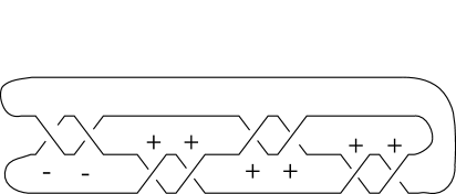
Figure 1: a non-alternating and non-positive diagram

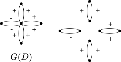
Figure 2: the graph $G(D)$ is homogeneous

Let $B_{n}$ be the braid group on $n$ strands with generators $\sigma_{1},\sigma_{2},\cdots,\sigma_{n-1}$. Stallings [31] introduced the notion of a homogeneous braid. A braid $\beta=\sigma_{i_{1}}^{\epsilon_{1}}\sigma_{i_{2}}^{\epsilon_{2}}\cdots\sigma_{i_{k}}^{\epsilon_{k}},\epsilon_{j}=\pm 1\ (j=1,\cdots,k)$ is homogeneous if

1. every $\sigma_{j}$ occurs at least once,

2. for each $j$, the exponents of all occurrences of $\sigma_{j}$ are the same.

For example, the braid $\sigma_{1}\sigma^{-1}_{2}\sigma_{1}\sigma^{-1}_{2}$ is homogeneous, however, the braid $\sigma^{2}_{1}\sigma_{2}\sigma_{1}\sigma^{-1}_{2}$ is not homogeneous. Stallings [31] proved that the closure of a homogeneous braid is fibered. The following lemma is origin of the name “homogeneous”.

Lemma 2.2 ([4]).

Let $\beta$ be a braid whose closure is a knot. Then $\beta$ is homogeneous if and only if the braid diagram of the closure of $\beta$ is homogeneous.

A knot $K$ is homogeneous if $K$ has a homogeneous diagram. The class of homogeneous knots includes alternating knots and positive knots. There are homogeneous knots which are non-alternating and non-positive and Cromwell [4] showed that the knot $9_{43}$ is the simplest one. One of the distinguished properties of a homogeneous diagram is the following.

Theorem 2.3 ([4]).

Let $D$ be a homogeneous diagram of a knot $K$. Then the genus of $K$ is realized by that of the Seifert surface obtained by applying Seifert’s algorithm to $D$.

Cromwell proved the above theorem algebraically. There is a geometric proof. Here we give an outline of the proof, which is suggested by M. Hirasawa.

The Seifert circles of a diagram is divided into two types: a Seifert circle is of type 1 if it does not contain any other Seifert circles in $\mathbb{R}^{2}$, otherwise it is of type 2. Let $D\subset\mathbb{R}^{2}$ be a knot diagram and $C$ a type 2 Seifert circle of $D$. Then $C$ separates $\mathbb{R}^{2}$ into two components $U$ and $V$ such that $U\cup V=\mathbb{R}^{2}$ and $U\cap V=\partial U=\partial V=C$. Let $D_{1}$ and $D_{2}$ be the diagrams formed form $D\cap U$ and $D\cap V$ by adding suitable arcs from $C$ respectively. If both $(U-C)\cap D\neq\emptyset$ and $(V-C)\cap D\neq\emptyset$, then $C$ decomposes $D$ into a $*$-product of $D_{1}$ and $D_{2}$, which is denoted by $D=D_{1}*D_{2}$. Then the Seifert surface obtained by applying Seifert’s algorithm to $D$ is a Murasugi sum of Seifert surfaces obtained by applying Seifert’s algorithm to $D_{1}$ and $D_{2}$ respectively (for the definition of a Murasugi sum, see [14] or [8]). A diagram is special if $D$ has no decomposing Seifert circles of type 2. A special positive (or negative) diagram is alternating. Cromwell implicitly showed the following (see Theorem 1 in [4]).

Lemma 2.4 ([4]).

Let $D$ be a homogeneous diagram of a knot $K$. Then
(1) there are special diagrams $D_{1},\cdots,D_{n}$ such that $D=D_{1}*D_{2}*\cdots*D_{n}$,
(2) each special diagram $D_{i}\ (i=1,\cdots,n)$ is the connected sum of special alternating diagrams,
(3) each special alternating diagram corresponds to a block of $G(D)$.

Let $D$ be homogeneous diagram of a knot $K$. Then, by Lemma 2.4, the Seifert surface $S$ obtained by applying Seifert’s algorithm to $D$ is Murasugi sums of the Seifert surfaces obtained by applying Seifert’s algorithm to the special alternating diagrams. The following lemma is classical results of Crowell and Murasugi.

Lemma 2.5.

Let $D$ be a alternating diagram of a knot $K$. Then the genus of $K$ is realized by that of the Seifert surface obtained by applying Seifert’s algorithm to $D$.

In [9], Gabai gave an elementary proof of Lemma 2.5 by using cut-and-past arguments. By Lemma 2.5, $S$ is Murasugi sums of minimal Seifert surfaces. Let $R_{1}$ and $R_{2}$ be two minimal Seifert surfaces. Then a Murasugi sum of $R_{1}$ and $R_{2}$ is a minimal Seifert surface due to Gabai [8]. Therefore we obtain a geometric proof of Theorem 2.3.

3 A characterization of a homogeneous diagram

In this section, we give a new characterization of a homogeneous diagram (Theorem 3.4). In particular, we show that if $D$ is a homogeneous diagram of a knot, then $\Delta(D)=0$. One can prove this by induction on the number of cut-vertices of $G(D)$, however, we prove this more graph-theoretically. For the Seifert Graph $G(D)$ associated to a knot diagram $D$, we construct a graph (which is denoted by $G(D)_{\Delta}$ later) such that the number of cycles of the graph is equal to $\Delta(D)$ and we prove if $D$ is homogeneous, then the graph has no cycles. By using Theorems 1.1 and 3.4, we determine the Rasmussen invariant of a homogeneous knot (Theorem 1.2).

Let $G_{+}$ and $G_{-}$ be the graphs which are obtained from a signed graph $G$ by removing all $-$ and $+$ edges, respectively. Here we note that, by definition, each vertex of $G$ belongs to exactly one connected component of $G_{+}$ and $G_{-}$ respectively. Let $G_{\Delta}$ be the graph whose vertices are the connected components of $G_{+}$ and $G_{-}$ and two vertices of $G_{\Delta}$ are connected by an edge if a vertex of $G$ belong to the two connected components (which correspond to the two vertices). We give two examples, which provide us the idea of the proof of Lemma 3.3.

Example 3.1.

Let $G(D)$ be the signed graph as in Figure 2. We label $1$ and $2$ the connected components of $G_{+}$ and $3$, $4$, $5$ and $6$ the connected components of $G_{-}$. Then $G_{\Delta}$ is the graph as in Figure 3 and it is tree.

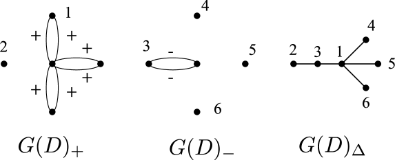
Figure 3: the graph $G_{\Delta}$ is tree

Example 3.2.

Let $G$ be the signed graph as in Figure 4. Then $G$ has only one block and it is $G$ itself. Since the block contains $+$ and $-$ edges, $G$ is not homogeneous. Note that $G$ has a cycle which contains $+$ and $-$ edges (in this case, the cycle is unique). We label $1$ and $2$ the connected components of $G_{+}$ and $3$, $4$, $5$ and $6$ the connected components of $G_{-}$. Then $G_{\Delta}$ is the graph as in Figure 4 and $G_{\Delta}$ has a cycle which is denoted by $(1,5)(5,2)(2,6)(6,1)$ (in this case, the cycle is also unique).

Conversely, let $\widetilde{e}_{1},\widetilde{e}_{2},\widetilde{e}_{3}$ and $\widetilde{e}_{4}$ be the edges of $G_{\Delta}$ and $\widetilde{v}_{1},\widetilde{v}_{2},\widetilde{v}_{3},\widetilde{v}_{4}$and $\widetilde{v}_{5}$ the vertices of $G_{\Delta}$ as in Figure 5. Let $v_{i}$ $(i=1,\cdots,4)$ be the vertex of $G$ which corresponds to $\widetilde{e}_{i}$ and let $v_{5}=v_{1}$. Then $\widetilde{v}_{i+1}$ as a connected component of $G_{+}$ or $G_{-}$ contains $v_{i}$ and $v_{i+1}$ and there exists a simple path $l_{i}$ in $\widetilde{v}_{i+1}$ from $v_{i}$ to $v_{i+1}$. Therefore we obtain a cycle $l_{1}l_{2}l_{3}l_{4}$ from $v_{1}$ to $v_{5}(=v_{1})$.

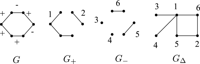
Figure 4: the graph $G$ is not homogeneous

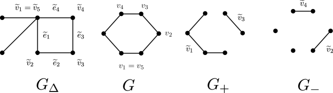
Figure 5: the graph $G$ is not homogeneous

For a signed graph $G$, we denote by sign$(e)$ the sign of an edge $e$ of $G$. We show the following lemma to prove Theorem 3.4. To prove $(2)\Longleftarrow(3)$ is essential.

Lemma 3.3.

Let $G$ be a signed graph. The following are equivalent.
(1) $G$ is not homogeneous.
(2) $G$ has a cycle which contains both $+$ and $-$ edges.
(3) $G_{\Delta}$ has a cycle.

Proof.

$(1)\Longrightarrow(2)$ Since $G$ is not homogeneous, by definition, there exists a block which contains $+$ and $-$ edges. Then there exist a vertex $v$ and edges $e_{1}$ and $e_{2}$ of the block such that one of the endpoints of $e_{1}$ and $e_{2}$ is $v$ respectively and sign($e_{1}$) $\neq$ sign($e_{2}$). Now $v$ is not a cut-vertex since $v$ is a vertex of the block. There $G$ has a cycle which contains both $+$ and $-$ edges.
$(1)\Longleftarrow(2)$ Let $e_{1}\cdots e_{n}$ be the cycle of $G$ which contains both $+$ and $-$ edges. Then there exists a natural number $i$ such that $\mathop{\mathrm{sign}}\nolimits(e_{i})\neq\mathop{\mathrm{sign}}\nolimits(e_{i+1})$. Let $v$ be the vertex such that one of the endpoints of $e_{i}$ and $e_{i+1}$ is $v$ respectively. Since $v$ is not a cut-vertex, edges $e_{i}$ and $e_{i+1}$ belong to the same block. Therefore $G$ is not homogeneous.
$(2)\Longrightarrow(3)$ Let $(e_{1}\cdots e_{i_{1}})\cdots(e_{i_{k-1}+1}\cdots e_{i_{k}})\cdots(e_{i_{j-1}+1}\cdots e_{i_{j}})$ be the cycle which contains both $+$ and $-$ edges, where $\mathop{\mathrm{sign}}\nolimits(e_{i_{k-1}+1})=\cdots=\mathop{\mathrm{sign}}\nolimits(e_{i_{k}})$ and $\mathop{\mathrm{sign}}\nolimits(e_{i_{k}})\neq\mathop{\mathrm{sign}}\nolimits(e_{i_{k}+1})$. Then the path $e_{i_{k-1}+1}\cdots e_{i_{k}}$ is also one in $G_{\mathop{\mathrm{sign}}\nolimits(e_{i_{k}})}$, which contracts to a vertex $\widetilde{v}_{k}$ of $G_{\Delta}$ $(k=1,\cdots,j)$. Let $\widetilde{e}_{k}$ be the edge of $G_{\Delta}$ whose endpoints are $\widetilde{v}_{k}$ and $\widetilde{v}_{k+1}$ $(k=1,\cdots,j-1)$, which is corresponding to the vertex $v_{k}$ such that one of the endpoints of $e_{i_{k}}$ and $e_{i_{k}+1}$ is $v_{k}$ respectively. Let $\widetilde{e}_{j}$ be the edge of $G_{\Delta}$ whose endpoints are $\widetilde{v}_{j}$ and $\widetilde{v}_{1}$, which is corresponding to the vertex $v_{j}$ such that one of the endpoints of $e_{i_{j}}$ and $e_{1}$ is $v_{j}$ respectively.

Therefore $\widetilde{e}_{1}\cdots\widetilde{e}_{j}$ is a path from $\widetilde{v}_{1}$ to $\widetilde{v}_{1}$, possibly not a cycle. If the path is not a cycle, we choose a cycle (as a subsequence of edges of the path). Therefore $G_{\Delta}$ has a cycle.
$(2)\Longleftarrow(3)$ Let $\widetilde{e}_{1}\cdots\widetilde{e}_{n}$ be the cycle $G_{\Delta}$ $(i=1,\cdots,n)$ and denote $\widetilde{e}_{i}=(\widetilde{v}_{i},\widetilde{v}_{i+1})$. Then $\widetilde{v}_{n+1}=\widetilde{v}_{1}$. Let $v_{i}$ be the vertex of $G$ which corresponds to $\widetilde{e}_{i}$ $(i=1,\cdots,n)$ and $v_{n+1}=v_{1}$. Recall that a vertex of $G_{\Delta}$ corresponds to a connected component of $G_{+}$ or $G_{-}$. Then $\widetilde{v}_{i+1}$ (as a connected component of $G_{+}$ or $G_{-}$) contain $v_{i}$ and $v_{i+1}$ $(i=1,\cdots,n)$. There exists a simple path $l_{i}$ from $v_{i}$ to $v_{i+1}$. There we obtain a path $l_{1}l_{2}\cdots l_{n}$ from $v_{1}$ to $v_{n+1}(=v_{1})$, possibly not a cycle. If the path is not a cycle, we choose a cycle (as a subsequence of edges of the path). By the construction, the cycle always contains both $+$ and $-$ edges. ∎

Note that $O_{+}(D)$ and $O_{-}(D)$ are equal to the numbers of connected components of $G(D)_{+}$ and $G(D)_{-}$, respectively. Therefore the number of vertices of $G(D)_{\Delta}$ is equal to $O_{+}(D)+O_{-}(D)$ and, by definition, the number of edges of $G(D)_{\Delta}$ is equal to $O(D)$. Lobb [20] showed that $\Delta(D)=b_{1}(G(D)_{\Delta})$ for any diagram $D$. For the completeness, we recall the proof here.

$$b_{1}(G(D)_{\Delta}) =b_{0}(G(D)_{\Delta})-\chi(G(D)_{\Delta})$$

$$=1-(O_{+}(D)+O_{-}(D)-O(D))$$

$$=\Delta(D),$$

where $b_{i}$ denotes the $i$-th Betti number $(i=0,1)$ and $\chi$ denotes the Euler characteristic. Then we obtain the following.

Theorem 3.4.

A diagram $D$ of a knot is homogeneous if and only if $\Delta(D)=0$.

Proof.

By the above argument, $\Delta(D)=0$ if and only if $G_{\Delta}$ is tree. Therefore the proof immediately follows from Lemma 3.3. ∎

Now we prove Theorem 1.2.

Proof of Theorem 1.2.

By Theorem 3.4, we obtain $\Delta(D)=0$. As mentioned before, Lobb [20] showed that if $\Delta(D)=0$, then $s(K)=w(D)-O(D)+2O_{+}(D)-1$. This completes the proof. ∎

4 Positivity of knots

In this section, we recall some notions of positivity and give some characterizations of a positive knot (Theorem 1.3). In particular, we recover Baader’s theorem which states that a knot is positive if and only if it is homogeneous and strongly quasipositive.

Let $D$ be a diagram of a knot. We denote by $D_{p}$ the diagram which is obtained from $D$ by smoothing (along the orientation of $D$) at a crossing $p$. A crossing of $D$ is nugatory if there exists a curve $l$ such that the intersection of $D$ and $l$ is only a crossing of $D$ (see also Figure 6). Then it is easy to see that the following lemma holds.

Figure 6: nugatory crossings

Lemma 4.1.

Let $p$ be a crossing of $D$. Then $p$ is nugatory if and only if the number of the connected components of $D_{p}$ is two.

Here we recall some notions of positivity for knots. A knot is braid positive if it is the closure of a braid of the form $\beta=\prod_{k=1}^{m}\sigma_{i_{k}}$. A knot is positive if it has a diagram without negative crossings. L. Rudolph introduced the concept of a (strongly) quasipositive knot (see [27]). Let

$$\sigma_{i,j}=(\sigma_{i},\cdots,\sigma_{j-2})(\sigma_{j-1})(\sigma_{i},\cdots,\sigma_{j-2})^{-1}.$$

A knot is strongly quasipositive if it is the closure of a braid of the form

$$\beta=\prod_{k=1}^{m}\sigma_{i_{k},j_{k}}.$$

A knot is quasipositive if it is the closure of a braid of the form

$$\beta=\prod_{k=1}^{m}\omega_{k}\sigma_{i_{k}}\omega_{k}^{-1},$$

where $\omega_{k}$ is a word in $B_{n}$. The following are known.

1. Let $K$ be a torus knot. Then $\tau(K)=s(K)/2=g_{*}(K)=g(K)$, where $g(K)$ denotes the (Seifert) genus of $K$. This is due to Rasmussen for $s$ [25] and Ozsváth and Szabó for $\tau$ [22]. These equalities provide a proof of the Milnor conjecture.

2. Let $K$ be a strongly quasipositive knot. Then $\tau(K)=s(K)/2=g_{*}(K)=g(K)$. This is due to Livingston [17].

3. Let $K$ be a quasipositive knot. Then $\tau(K)=s(K)/2=g_{*}(K)$. This is due to Plamenevskaya [23] and Hedden (with a detailed and constructive proof) [10] for $\tau$, and Plamenevskaya [24] and Shumakovitch [30] for $s$.

By using Lemma 4.1, we prove Theorem 1.3.

Proof of Theorem 1.3.

$(1)\Longrightarrow(2)$ A positive knot is strongly quasipositive ([21] and [28]).
$(2)\Longrightarrow(3)$ A strongly quasipositive knot $K$ is a quasipositive knot with $g_{*}(K)=g(K)$ [27].
$(3)\Longrightarrow(4)$ Since $K$ is a quasipositive knot, $\tau(K)=s(K)/2=g_{*}(K)$. By the assumption, $g_{*}(K)=g(K).$ Therefore $\tau(K)=s(K)/2=g_{*}(K)=g(K)$.
$(4)\Longrightarrow(1)$ Let $D$ be a homogeneous diagram of $K$. Then the genus of $K$ is realized by that of the surface constructed by applying Seifert’s algorithm to $D$ (Theorem 2.3). Therefore $2g(K)=1+c(D)-O(D)$, where $c(D)$ denotes the number of crossings of $D$. By Theorem 1.2, we have $s(K)=w(D)-O(D)+2O_{+}(D)-1$. By assumption, $s(K)=2g(K)$. This implies that $O_{+}(D)-1=n_{-}(D)$, where $n_{-}(D)$ denotes the number of negative crossings of $D$.

If there exists a non-nugatory negative crossing $p$ of $D$, then $D_{p}$ is connected by Lemma 4.1. Therefore $O_{+}(D)-1<n_{-}(D)$ (since, in general, the difference of the numbers of the connected components of two link diagrams $D_{1}$ and $D_{2}$ such that $D_{2}$ is obtained from $D_{1}$ by smoothing at a crossing of $D_{1}$ is $0$ or $1$). This contradicts the fact that $O_{+}(D)-1=n_{-}(D)$. Therefore all negative crossings of $D$ are nugatory and $D$ represents a positive knot. ∎

Corollary 1.4 immediately follows from Theorem 1.3.

5 A new approach to estimate the Rasmussen invariant of a knot

Let $D$ be a diagram of a knot with $\Delta(D)\neq 0$. Then Kawamura-Lobb’s inequality may not be sharp as follow.

Example 5.1.

Let $K$ be the pretzel knot of type $(3,-5,-7)$ and $D$ the standard pretzel diagram of $K$. Then $\omega(D)=9,O(D)=14,O_{+}(D)=3$ and $O_{-}(D)=11$. Therefore $\Delta(D)=1$ and $w(D)-O(D)+2O_{+}(D)-1=0$. On the other hand, since $K$ is strongly quasipositive [29], we obtain $s(K)=2g_{*}(K)=2g(K)=2$. Remark that $K$ is topologically slice but not smoothly slice.

We need a more shaper estimation to describe the Rasmussen invariant of the pretzel knot of type $(3,-5,-7)$ in terms of its standard pretzel diagram. Roughly speaking, there are two approaches to estimate or determine the Rasmussen invariant. One of them is to compute the Khovanov homology by using a computer and to use the spectral sequence which converges to Lee’s homology. The other is to use some formal properties of the Rasmussen invariant (and the tau invariant). We propose a new and direct approach to estimate or determine the Rasmussen invariant. We briefly recall the definition of the Rasmussen invariant to explain this. For a full explanation, see [25].

Let $D$ be a diagram of a knot $K$ and $C_{Lee}^{*}(D)$ Lee’s complex (see [25] for the definition). Then Lee [16] proved that the homology group of $C_{Lee}^{*}(D)$ is independent of the choice of diagrams of $K$. Lee’s homology of $K$, denoted by $H_{Lee}^{*}(K)$, is defined to be the homology group of $C_{Lee}^{*}(D)$. In addition, for a diagram $D$ of a knot $K$, Lee [16] associated two (co)cycles of $C_{Lee}^{*}(D)$, denoted by $f_{o}$ and $f_{\bar{o}}$, and proved that $[f_{o}]$ and $[f_{\bar{o}}]$ are a basis of $H_{Lee}^{*}(K)$, in particular, that the dimension of $H_{Lee}^{*}(K)$ is equal to two, where [$\cdot$] denotes its homology class. This basis is called canonical since the basis is determined up to multiple of $2^{c}$ for $K$ [25], where $c$ is an integer.

Rasmussen [25] defined a filtration grading $q$ on a non-zero element of $C_{Lee}^{*}(D)$ (which induces a filtration on $C_{Lee}^{*}(D)$). Then a filtration grading $s$ on a non-zero element $[x]$ of $H_{Lee}^{*}(K)$ (which also induces a filtration on $H_{Lee}^{*}(K)$) is defined as follows.

$$s([x])=\max\{q(y)|[x]=[y]\}.$$

Then the Rasmussen invariant of $K$, denoted by $s(K)$, is defined to be $s([f_{o}])+1(=s([f_{\bar{o}}])+1)$.

Since $s([f_{o}])\geq q(f_{o})$ and $q(f_{o})=\omega(D)-O(D)$ (by the definition of $q$), we obtain $s(K)\geq\omega(D)-O(D)+1$. This is the slice-Bennequin inequality for the Rasmussen invariant for $K$ (see [24] and [30]). Theorem 1.1 implies that there exists a cycle $f$ such that $[f_{o}]=[f]$ and $q(f)=\omega(D)-O(D)+2O_{+}(D)-2$, however, yet no one has succeeded to describe $f$ explicitly. In [1], as a first step toward this, we describe a cycle $f_{1}$ with $[f_{o}]=[f_{1}]$ which gives the so-called shaper slice-Bennequin inequality for the Rasmussen invariant of a knot [12] (which is stronger than the slice-Bennequin inequality and weaker than the inequality of Kawamura and Lobb, see [13]). In the future work, the graph $G(D)_{\Delta}$ is expected to play an important role (see also [6]). We conclude this paper by giving the following problem.

Problem. Let $D$ be the standard diagram of $P(3,-5,-7)$. Find a cycle $f$ of $C_{Lee}^{*}(D)$ such that $[f_{o}]=[f]$ and $q(f)=\omega(D)-O(D)+2O_{+}(D)=1$.

References

- [1] T. Abe, A cycle of Lee’s homology of a knot, preprint.
- [2] S. Baader, Quasipositivity and homogeneity, Math. Proc. Cambridge Philos. Soc. 139 (2005), no. 2, 287–290.
- [3] Cornelia A. Van Cott, Ozsváth-Szabó and Rasmussen invariants of cable knots, arXiv:0803.0500v2 [math.GT].
- [4] P. R. Cromwell, Homogeneous links, J. London Math. Soc. (2) 39 (1989), no. 3, 535–552.
- [5] P. R. Cromwell, Knots and Links, Cambridge University Press, (2004).
- [6] A. Elliott, State Cycles, Quasipositive Modification, and Constructing H-thick Knots in Khovanov Homology, arXiv:0901.4039v2 [math.GT].
- [7] M. Freedman, R. Gompf, S. Morrison, K. Walker, Man and machine thinking about the smooth 4-dimensional Poincaré conjecture,arXiv:0906.5177v2 [math.GT].
- [8] D. Gabai, The Murasugi sum is a natural geometric operation, Low-dimensional topology (San Francisco, Calif., 1981), 131–143, Contemp. Math., 20, Amer. Math. Soc., Providence, RI, 1983.
- [9] D. Gabai, Genera of the alternating links, Duke Math. J. 53 (1986), no. 3, 677–681.
- [10] M. Hedden, Notions of positivity and the Ozsváth-Szabó concordance invariant, arXiv:math/0509499v1 [math.GT].
- [11] M. Hedden and P. Ording, The Ozsváth-Szabó and Rasmussen concordance invariants are not equal, Amer. J. Math. 130 (2008), no. 2, 441–453.
- [12] T. Kawamura, The Rasmussen invariants and the sharper slice-Bennequin inequality on knots, Topology 46 (2007), no. 1, 29–38.
- [13] T. Kawamura, An estimate of the Rasmussen invariant for links, preprint (2009).
- [14] A. Kawauchi, A survey of knot theory, Birkhäuser-Verlag, Basel (1996).
- [15] M. Khovanov, A categorification of the Jones polynomial, Duke Math. J. 101 (2000), no. 3, 359–426.
- [16] E. S. Lee, An endomorphism of the Khovanov invariant, Adv. Math. 197 (2005), no. 2, 554–586.
- [17] C. Livingston, Computations of the Ozsváth-Szabó knot concordance invariant, Geom. Topol. 8 (2004) 735–742.
- [18] C. Livingston and S. Naik, Ozsváth-Szabó and Rasmussen invariants of doubled knots, Algebr. Geom. Topol. 6 (2006), 651–657.
- [19] C. Livingston, Slice knots with distinct Ozsváth-Szabó and Rasmussen invariants, Proc. Amer. Math. Soc. 136 (2008), no. 1, 347–349.
- [20] A. Lobb, Computable bounds for Rasmussen’s concordance invariant, arXiv:0908.2745v2 [math.GT].
- [21] T. Nakamura, Four-genus and unknotting number of positive knots and links, Osaka J. Math. 37 (2000), no. 2, 441-451.
- [22] P. Ozsváth and Z. Szabó, Knot Floer homology and the four-ball genus, Geom. Topol. 7 (2003), 615–639.
- [23] O. Plamenevskaya, Bounds for the Thurston-Bennequin number from Floer homology, Algebr. Geom. Topol. 4 (2004), 399–406.
- [24] O. Plamenevskaya, Transverse knots and Khovanov homology, Math. Res. Lett. 13 (2006), no. 4, 571–586.
- [25] J. Rasmussen, Khovanov homology and the slice genus, to appear in Invent. Math.
- [26] J. Rasmussen, Floer homology and knot complements, arXiv:math.GT/0306378.
- [27] L. Rudolph, Knot theory of complex plane curves, Handbook of knot theory, 349–427, Elsevier B. V., Amsterdam, (2005).
- [28] L. Rudolph, Positive links are strongly quasipositive, Geometry Topology Monographs 2 (1999), Proceedings of the Kirbyfest, paper no. 25, 555–562.
- [29] L. Rudolph, Quasipositivity as an obstruction to sliceness, Bull. Amer. Math. Soc. (N.S.) 29 (1993), no. 1, 51–59.
- [30] A. Shumakovitch, Rasmussen invariant, slice-Bennequin inequality, and sliceness of knots math, J. Knot Theory Ramifications 16 (2007), no. 10, 1403–1412.
- [31] J. Stallings, Constructions of fibred knots and links, Algebraic and geometric topology (Proc. Sympos. Pure Math., Stanford Univ., Stanford, Calif., 1976), Part 2, pp. 55–60, Proc. Sympos. Pure Math., XXXII, Amer. Math. Soc., Providence, R. I., 1978.
- [32] A. Stoimenow, Some examples related to knot sliceness, J. Pure Appl. Algebra 210 (2007), no. 1, 161–175.