Evolutionary advantage of small populations on complex fitness landscapes

Abstract

Recent experimental and theoretical studies have shown that small asexual populations evolving on complex fitness landscapes may achieve a higher fitness than large ones due to the increased heterogeneity of adaptive trajectories. Here we introduce a class of haploid three-locus fitness landscapes that allow the investigation of this scenario in a precise and quantitative way. Our main result derived analytically shows how the probability of choosing the path of the largest initial fitness increase grows with the population size. This makes large populations more likely to get trapped at local fitness peaks and implies an advantage of small populations at intermediate time scales. The range of population sizes where this effect is operative coincides with the onset of clonal interference. Additional studies using ensembles of random fitness landscapes show that the results achieved for a particular choice of three-locus landscape parameters are robust and also persist as the number of loci increases. Our study indicates that an advantage for small populations is likely whenever the fitness landscape contains local maxima. The advantage appears at intermediate time scales, which are long enough for trapping at local fitness maxima to have occurred but too short for peak escape by the creation of multiple mutants.

KEY WORDS: clonal interference, finite population, fitness landscape, fixation probability, three-locus models

Running Title : Advantage of small populations

Contact Information (for all authors)

Kavita Jain

postal address: Theoretical Sciences Unit and Evolutionary and Organismal Biology Unit, Jawaharlal Nehru Centre for Advanced Scientific Research, Jakkur P.O., Bangalore 560064, India

work telephone number: +91-80-22082948

E-mail:jain@jncasr.ac.in

Joachim Krug

postal address: Institute für Theoretische Physik, Universität zu Köln, Zülpicher Str. 77, 50937 Köln, Germany

work telephone number: +49-221-470-2818

E-mail:krug@thp.uni-koeln.de

Su-Chan Park (Corresponding Author)

address: Department of Physics, The Catholic University of Korea, 43-1 Yeokgok 2-dong, Wonmi-gu, Bucheon 420-743, Republic of Korea

work telephone number: +82-2-2164-4524

E-mail: spark0@catholic.ac.kr

Consider a population experiencing a recent environmental change. Assuming that the population is ill-adapted to the new environment, as is typically the case in the beginning of an evolution experiment (Lenski and Travisano, 1994), the adaptation to the new environment relies on the supply of beneficial mutations available to the population. During the early stages of adaptation, it is a good approximation to assume that the supply of beneficial mutations is unlimited. Then as the rate at which the beneficial mutations appear is given by the mutation rate per individual times the population size, a large population is expected to experience more beneficial mutations and hence adapt faster than a small population.

This conclusion does not seem to depend on the topography and epistatic interactions in the fitness landscape. If the fitness landscape is non-epistatic in the sense that (beneficial) mutations act multiplicatively on fitness, a large population adapts faster than a small population, although this advantage is strongly reduced in asexuals due to clonal interference (Gerrish and Lenski, 1998; de Visser et al., 1999; Wilke, 2004; Park and Krug, 2007; Park et al., 2010). Even if the fitness landscape is highly epistatic such as a maximally rugged (house-of-cards) landscape (Kingman, 1978), a large population still wins on average (Park and Krug, 2008). This leaves the question as to whether small populations might be at an advantage in complex fitness landscapes with an intermediate degree of epistasis and ruggedness.

In a recent experimental work (Rozen et al., 2008) studying the adaptation dynamics of populations of E. coli in simple and complex nutrient environments, it was found that small populations could attain higher fitness than large populations in a complex medium which can be expected, on general grounds, to give rise to a rugged and epistatic fitness landscape. The observed fitness advantage of small populations was associated with a greater heterogeneity in their adaptive trajectories compared to large populations. Specifically, small populations that eventually reached the highest fitness levels were often the ones that initially displayed a rather shallow fitness increase, whereas the fitness of those that gained a large initial advantage tended to level off quickly. In large populations trajectories were more uniform and typically showed a rapid initial fitness increase followed by a significant slowing down or saturation.

These experiments suggest that an adaptive advantage can arise from the higher level of stochasticity in the incorporation of beneficial mutations displayed by small populations, provided the topography of the underlying fitness landscape is sufficiently complex. As the detailed structure of the experimental fitness landscape is unknown and unfeasible to determine, it is useful to investigate this mechanism theoretically. In previous work this was done using extensive simulations for a class of random fitness landscapes with tunable ruggedness (Handel and Rozen, 2009). The main conclusion from this study was that an advantage of small populations can be observed in a substantial fraction of random landscapes, but the dependence of the effect on parameters such as the population size, the mutation rate and the fitness effect of beneficial mutations was not explored systematically.

In this article, we introduce a minimal, analytically tractable model which captures the dynamic behavior of the population fitness in the experiments by Rozen et al. (2008). We show that the simplest fitness landscape that can exhibit a small population advantage is a haploid, diallelic three-locus landscape where the genotypes of minimal and maximal fitness are separated by three mutational steps. There are then 3! = 6 distinct shortest paths leading from the global fitness minimum (the wild type) to the global maximum, corresponding to the different orderings in which the mutations are introduced into the population (Gokhale et al., 2009). We distinguish between smooth paths along which fitness increases monotonically, and rugged paths containing at least one deleterious mutation. The three-locus landscape is constructed in such a way that the rugged paths contain a local fitness maximum, and they confer the greatest initial fitness increase to a population initially fixed for the minimal fitness genotype.

The existence of rugged paths is the hallmark of sign epistasis, a specific type of genetic interaction under which a given mutation can be beneficial or deleterious depending on the genetic background (Weinreich et al., 2005; Poelwijk et al., 2007). Sign epistasis implies that at least some of the mutational pathways leading to the global maximum of the fitness landscape are rugged, and thus inaccessible to an adaptive dynamics that is constrained to increase fitness in each step. In addition, sign epistasis is a necessary (but not sufficient) condition for the existence of multiple fitness maxima (Poelwijk et al., 2011). The presence of sign epistasis was established in several recent experimental studies, where all combinations of a selected set of individually beneficial or deleterious mutations were constructed and their fitness effects (or some proxy thereof) were measured (Weinreich et al., 2006; Lozovsky et al., 2009; de Visser et al., 2009; Carneiro and Hartl, 2010). There is also considerable evidence for the existence of multiple fitness maxima from evolution experiments using bacterial and viral populations (Korona et al., 1994; Burch and Chao, 1999, 2000; Elena and Lenski, 2003). It is therefore reasonable to assume that sign epistasis and mulitple fitness maxima are present also in the complex environment considered by Rozen et al. (2008).

The analysis presented below shows that the speed of adaptation is generally an increasing function of population size both along smooth and along rugged paths. However, the probability with which a particular type of path is chosen depends on population size in such a way that small populations can be favored at least over a certain range of time scales. In particular, as we shall show, the probability to choose the rugged path in the three-locus model rises sharply with the onset of clonal interference, and it approaches unity when the dynamics becomes completely deterministic for very large populations, because then the mutation with the largest initial fitness increase is certain to fix (Jain and Krug, 2007b). The dynamics of small populations are less predictable, and they therefore enjoy an advantage by more frequently avoiding getting trapped at the local fitness maximum. The main part of the article is devoted to a detailed, quantitative analysis of this scenario. We then show that the mechanism identified within the specific three-locus model is robust by simulating populations on variants of the house-of-cards fitness landscape with three or more loci, and conclude the paper with a discussion of our key results.

Models

Fitness landscapes

In the main part of this work we consider the space of genotypes composed of three loci with two alleles each, which will be denoted $0$ and $1$. Each genotype is assigned a fitness $W$ according to

$$W(000) = 1$$

$$W(001) = W(010)=1+s_{1}$$

$$W(100) = 1+s_{2}$$

$$W(011) = W(101)=W(110)=(1+s_{1})^{2}$$

$$W(111) = (1+s_{1})^{3}$$ (1)

where $s_{2}>s_{1}>0$ and $(1+s_{1})^{2}<1+s_{2}<(1+s_{1})^{3}$. Thus there is a local fitness maximum at genotype $\{100\}$ and the global maximum is located at genotype $\{111\}$.

In addition to the landscape equation (1), we consider two ensembles of random fitness landscapes consisting of $L$-locus genotypes with two alleles at each site. In the first ensemble referred to as unconstrained ensemble, the least fit genotype is assigned the allele $0$ at every locus and fitness $1$ while the rest of the genotypes are given fitnesses

$$W(\textrm{genotype})=1+Sx,$$ (2)

where $S$ controls the strength of selection and $x$ is a random number drawn from an exponential distribution with mean $1$. This is Kingman’s house-of-cards model adapted to a finite number of diallelic loci (Kingman, 1978; Kauffman and Levin, 1987; Jain and Krug, 2007b; Park and Krug, 2008). It is also instructive to study a constrained version of the above model in which the fittest genotype has all loci with allele 1 (Klözer, 2008; Carneiro and Hartl, 2010). Such landscapes are generated by assigning the maximum value amongst $2^{L}-1$ random numbers given by equation (2) as the fitness of the antipodal point of the least fit genotype in the genotype space. Note that these landscapes have exactly the same statistics as those which are sampled under the condition that the antipodal genotype is the fittest among all randomly generated landscapes by equation (2).

Population dynamics

We mainly work with a finite population of size $N$ which evolves according to standard Wright-Fisher dynamics in discrete generations. In each generation, an offspring chooses a parent with a probability proportional to the parent’s fitness and copies the parent’s genotype. Then the point mutation process is implemented symmetrically in which $0\leftrightarrow 1$ with probability $\mu$. This process is repeated until all $N$ offspring have been generated. In the actual simulations, we treated the population size of each genotype as a random variable which is sampled according to a multinomial distribution; for details see Park and Krug (2007).

It is also useful to compare the results obtained for finite $N$ with the predictions of the deterministic mutation-selection dynamics of “quasispecies” type which applies for infinite populations (Bürger, 2000; Jain and Krug, 2007a). This is done by iterating the deterministic evolution equations for the frequencies $f(\sigma,t)$ of genotype $\sigma$ at generation $t$, which read

$$f(\sigma,t+1)=\frac{\sum_{\sigma^{\prime}}M(\sigma\leftarrow\sigma^{\prime})W(\sigma^{\prime})f(\sigma^{\prime},t)}{\sum_{\sigma^{\prime}}W(\sigma^{\prime})f(\sigma^{\prime},t)}.$$ (3)

Here $M(\sigma\leftarrow\sigma^{\prime})=\mu^{d(\sigma,\sigma^{\prime})}(1-\mu)^{L-d(\sigma,\sigma^{\prime})}$ is the probability that an $L$-locus genotype $\sigma^{\prime}$ mutates to genotype $\sigma$ at Hamming distance $d(\sigma,\sigma^{\prime})$.

Results

Evolution time scales

We begin by a comparison of the time taken to reach the global maximum along the smooth and the rugged paths on the fitness landscape defined by equation (1). A population that is initially fixed for the minimum fitness genotype $\{000\}$ has a choice between three single site mutations. Two of these (to genotypes $\{001\}$ and $\{010\}$) lead the population to a smooth path towards the global fitness maximum $\{111\}$, whereas the third leads to the local fitness maximum $\{100\}$ from which the population can escape only by the creation of a double mutant (Iwasa et al., 2004; Weinreich and Chao, 2005; Weissman et al., 2009).

We estimate the time scales of the relevant evolutionary processes in the strong selection weak mutation (SSWM) regime (Gillespie, 1983, 1984; Orr, 2002), where $N\mu\ll 1$ and the population is monomorphic almost all the time. For simplicity, in the present discussion we neglect back mutations towards the wild type genotype $\{000\}$. Starting from the wild type, each of the single step mutants is generated in the population at rate $N\mu$ and goes to fixation with probability $\pi(s)$ given by (Kimura, 1962)

$$\pi(s)\approx\frac{1-e^{-2s}}{1-e^{-2Ns}}$$ (4)

with $s=s_{1}$ or $s_{2}$. For $N^{-1}\ll s\ll 1$, the fixation probability $\pi(s)\approx 2s$. The waiting times for low fitness ($T_{1}$) and high fitness ($T_{2}$) mutants that will ultimately fix are therefore

$$T_{1}\approx\frac{1}{2\mu Ns_{1}},\;\;\;T_{2}\approx\frac{1}{2\mu Ns_{2}}.$$ (5)

Adaptation along one of the smooth paths proceeds by sequentially fixing two additional beneficial mutations with selection coefficient $s_{1}$, and the total evolution time is therefore $T_{\mathrm{smooth}}\approx 3T_{1}$.

By contrast, populations that choose the rugged path need to escape from the local fitness peak $\{100\}$ in order to reach the global maximum. The corresponding escape time can be estimated along the lines of Weinreich and Chao (2005). Following these authors we introduce the selection coefficients

$$s_{\mathrm{ben}}=\frac{W(111)}{W(100)}-1\approx 3s_{1}-s_{2},\;\;\;s_{\mathrm{del}}=\frac{W(100)}{W(101)}-1\approx s_{2}-2s_{1}$$ (6)

which express the relative fitness advantage of the global maximum compared to the local peak ($s_{\mathrm{ben}}$) and that of the valley genotypes compared to the local peak ($s_{\mathrm{del}}$), respectively. Depending on the population size, the peak escape can proceed through two distinct pathways. In populations smaller than a critical size $N_{c}$ (Weinreich and Chao, 2005), the two mutations separating the genotypes $\{100\}$ and $\{111\}$ fix sequentially, while in larger populations they fix simultaneously. We are interested in population size $\gg N_{c}\approx\ln(s/\mu)/s$ which can be easily satisfied in the SSWM regime as $Ns\gg 1$. In the simultaneous mode the escape time is given approximately by

$$T_{\mathrm{esc}}\approx\frac{s_{\mathrm{del}}}{4N\mu^{2}s_{\mathrm{ben}}}.$$ (7)

Assuming all selection coefficients $s_{1},s_{2},s_{\mathrm{ben}},s_{\mathrm{del}}$ to be of a similar magnitude $s$, we see that

$$\frac{T_{\mathrm{esc}}}{T_{1,2}}\sim\frac{s}{\mu}\gg 1$$ (8)

whenever $\mu\ll s$, which is expected to hold under most conditions. In particular, it is true in the SSWM regime because $N\mu\ll 1$ and $Ns\gg 1$. Equation (8) implies that the evolution time $T_{\mathrm{rugged}}$ along a rugged path is dominated by the escape time $T_{\mathrm{esc}}$, and is much larger than $T_{\mathrm{smooth}}$. However, both equation (5) and equation (7) share the same dependence on population size $N$, so once the type of evolutionary path is chosen, a large population is always at a relative advantage.

Mean fitness evolution and heterogeneous adaptive trajectories

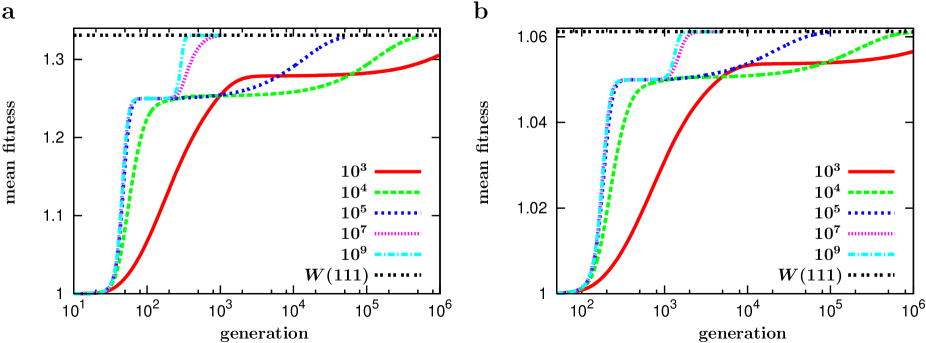
Figure 1: Average fitness as a function of time on the fitness landscape defined by equation (1) for $\mu=10^{-5}$, (a) $s_{1}=0.1$, $s_{2}=0.25$ and (b) $s_{1}=0.02$, $s_{2}=0.05$, and various population sizes indicated in the figures. As a guide to the eye, the maximum fitness values $W(111)$ for each case are also drawn. The data have been averaged over $10^{5}$ histories. Fitness increases with population size at short times and at long times, but in both cases this relationship is reversed for a range of population sizes at intermediate times.

Figure 1 shows the evolution of the population fitness obtained from simulations of the Wright-Fisher model in the landscape defined by equation (1). Each curve contains data averaged over many stochastic histories for a given value of $N$, keeping other parameters fixed, and starting with all individuals at the genotype $\{000\}$ with lowest fitness. At short times the fitness rises more rapidly for larger populations, as expected on the basis of the estimates given in equation (5) for $N\mu\ll 1$, while for $N\mu>1$ fitness becomes independent of $N$. Large populations are also seen to be at an advantage for extremely long times, beyond $10^{5}$ generations. However, for both parameter sets displayed in the figure, the ordering of fitness with increasing population size is reversed in an intermediate time interval, which begins at around 2000 generations.

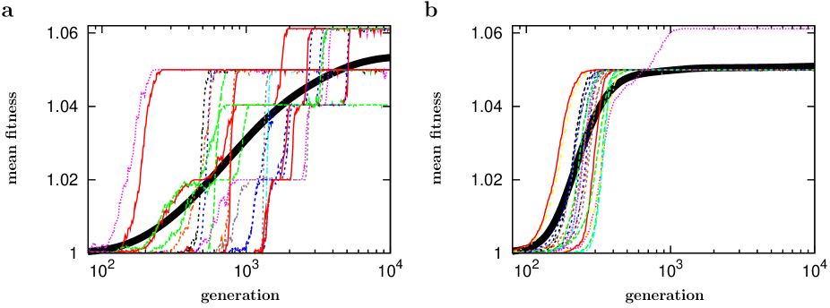
Figure 2: Population mean fitness as a function of time for 20 histories on the fitness landscape equation (1). The population size is (a) $N=10^{3}$ and (b) $10^{4}$, the selection coefficients are $s_{1}=0.02$ and $s_{2}=0.05$ and the mutation probability is $\mu=10^{-5}$ (same as in Figure 1(b)). The smooth curves depict the average over $10^{5}$ independent runs.

The origin of this reversal is illustrated in Figure 2, which shows individual fitness trajectories for the parameter set of Figure 1 (b) and two different population sizes. Individual fitness trajectories display a step-like behavior, which reflect the transitions in the most populated genotype. In particular, populations in which the local peak genotype $\{100\}$ becomes dominant are seen to remain trapped at the local peak for a long time (compare to equation (7)). Although the initial rise in fitness is much faster for the large populations than for the small ones, the fraction of trajectories that take the rugged path (and thus get trapped at the local peak) also increases with increasing $N$, from 11/20 in the Figure 2(a) ($N=10^{3}$) to 19/20 in Figure 2(b) ($N=10^{4}$). As a consequence, the fitness after $10^{4}$ generations, when averaged over all trajectories, is larger for the small populations than for the large ones. Similar to the experimental observations of Rozen et al. (2008) and the simulations of Handel and Rozen (2009), smaller populations reach a higher fitness level because their adaptive trajectories are more heterogeneous, allowing them to avoid trapping at the local fitness peak in a larger number of trials.

Path probability

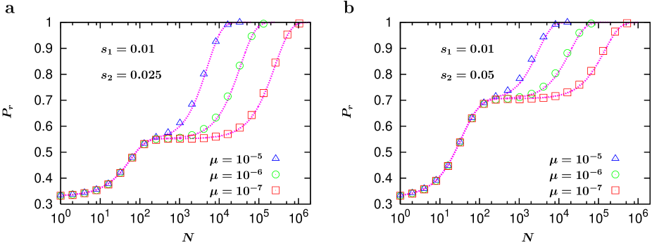
Figure 3: Fixation probability $P_{r}$ of the allele $C$ for the simplified three alleles system obtained using numerical simulations for $\mu=10^{-5}$ (triangles), $10^{-6}$ (circles), and $10^{-7}$ (squares). Dotted lines show the analytic prediction of equations (18,19).

To quantify the statement that large populations are more likely to take the rugged path, we introduce the probability $P_{r}(N)$ that the rugged path is taken by a population of size $N$. In simulations, the probability $P_{r}$ was measured by counting the number of events in which $\{100\}$ becomes the most populated genotype for the first time. In Figure 3 these numerical results are compared with the analytical expressions (discussed below) and the two are seen to be in very good agreement. We see that $P_{r}$ generally increases with $N$ (provided $\mu$ is not too small) thus supporting our main contention. Before presenting an analytic calculation of $P_{r}$ covering the full range of population sizes, we discuss the limiting cases of very small and very large populations.

SSWM regime: $N\mu\ll 1$

When $N\mu\ll 1$, the path probability $P_{r}$ is equal to the probability that the first mutant that will be fixed in a population initially monomorphic for the genotype $\{000\}$ is the local peak genotype $\{100\}$. That is,

$$P_{r}|_{N\mu\ll 1}=\frac{\pi(s_{2})}{\pi(s_{2})+2\pi(s_{1})}.$$ (9)

When selection is weak, in the sense of $Ns_{1,2}\ll 1$, the fixation probability is given by its neutral value $\pi=1/N$ and we obtain $P_{r}=1/3$. On the other hand, for strong selection (and assuming that $s_{1,2}\ll 1$) we have

$$P_{r}^{SSWM}\approx\frac{s_{2}}{s_{2}+2s_{1}}$$ (10)

independent of $N$, which is equal to 0.54 and 0.56, respectively, in the two cases displayed in Figure 1.

Deterministic quasispecies regime: $N\to\infty$

For very large populations the local peak mutant is always present in the population in considerable numbers and can therefore be expected to dominate the population with a probability approaching unity (Jain and Krug, 2007b). The quantitative analysis of this case is based on the deterministic infinite population dynamics defined by equation (3). As the initial population is assumed to be fixed at the genotype $\{000\}$, for small mutation rates equation (3) gives $f(\sigma,t=1)\sim\mu^{d(\sigma,000)}$ which is the same for all genotypes at constant Hamming distance from $\{000\}$. For $t>1$, the genotypic population can be determined by a simple construction described by Jain and Krug (2005) and Jain (2007) in which the population of a genotype increases exponentially with its fitness, starting from $f(\sigma,1)$.

For our fitness landscape, as the population frequencies $f(111,1)<f(100,1)$ but the fitness values $W(111)>W(100)$, it is possible that the genotype $\{111\}$ becomes the most populated one before $\{100\}$ thus bypassing the local maximum. The population at sequence $\{100\}$ overtakes that of $\{000\}$ at time $t_{1}$ when $f(000,t_{1})=f(100,t_{1})$, which on using $f(\sigma,t)\propto\mu^{d(\sigma,000)}W(\sigma)^{t}$ gives $t_{1}=-\ln\mu/\ln W(100)$. Similarly the time $t_{2}$ at which the population of the global maximum overtakes that of the initial sequence is given by $t_{2}=-3\ln\mu/\ln W(111)$. Thus the condition for bypassing corresponding to $t_{2}<t_{1}$ reads

$$W^{3}(100)<W(111)\Leftrightarrow s_{2}<s_{1}$$ (11)

which is ruled out by construction. Thus bypassing cannot occur and we conclude that

$$\lim_{N\to\infty}P_{r}(N)=1.$$ (12)

Clonal interference regime

The phenomenon of interest in this paper occurs in the intermediate range of population sizes where $P_{r}$ increases from its small population value in equation (9) to the large population limit in equation (12). This regime is more difficult to analyze because of the presence of multiple competing mutant clones in the population. To find an analytic expression for $P_{r}(N)$ in this regime, we first reduce the three-locus problem into a single locus with three alleles, say $A$ , $B$, and $C$ with respective fitness 1, $1+s_{1}$, and $1+s_{2}$. The two genotypes $\{010\}$ and $\{001\}$ are lumped into a single allele $B$. The mutation from $A$ to $B$ occurs with probability $2\mu$ and that from $A$ to $C$ with $\mu$. No other mutation is possible, which ensures that either $B$ or $C$ will be eventually fixed. It is clear that the fixation probability of allele $B$ approximates $1-P_{r}$.

We now present an approximate calculation of $P_{r}$ for the three-allele model using ideas from clonal interference theory. At time zero the population is monomorphic for allele $A$. We would like to determine the probability that an allele $B$ which originates at some time $t_{0}>0$ fixes at a later time $t_{0}+t_{f}$. It is plausible to assume that the fixation and origination of a mutation are not correlated, and hence to treat the two processes separately.

Let us first consider the probability $p_{1}(t)$ for the allele $B$ to originate at time $t$. An allele $B$ appears in the population at rate $2N\mu$ and would, in the absence of other mutations, go to fixation with probability $\pi(s_{1})$. As is customary in the field (Maynard Smith, 1971; Gerrish and Lenski, 1998; Desai and Fisher, 2007), we interpret the fixation probability $\pi$ as the probability for the mutant population to survive genetic drift and, thus, to reach a size large enough for the further time evolution to be essentially deterministic. Mutations of type $B$ which reach this level are called contending mutations (Gerrish, 2001), and they arise at rate $2N\mu\pi(s_{1})$. To obtain $p_{1}(t)$ this rate has to be multiplied with the probability that the contending mutation in question is the first to appear among all possible contenders for fixation. To estimate the probability that no contending mutation (of any type) has appeared before time $t$, we use a Poisson approximation in which the probability for the non-occurrence of an event is the negative exponential of the expected number of events. Since the expected number of contending mutations arising up to time $t$ is $N\mu(\pi(s_{2})+2\pi(s_{1}))t$, we conclude that

$$p_{1}(t)=2N\mu\pi(s_{1})\exp(-N\mu(\pi(s_{2})+2\pi(s_{1}))t).$$ (13)

We next determine the probability $p_{2}$ that the fixation of the contending mutation of type $B$ is not impeded by the appearance of a contending mutation of type $C$ at some time larger than $t_{0}$. Such a mutation can only arise from the wildtype population $A$. According to our assumptions, the evolution of the frequency $x$ of $B$ alleles after time $t_{0}$ follows the deterministic, logistic growth equation

$$\frac{dx}{dt}=s_{1}x(1-x).$$ (14)

The expected number of $C$ alleles that arise from the wildtype population until the fixation time $t_{f}$ is therefore

$$\int_{0}^{t_{f}}N\mu(1-x(t))dt=\int_{x_{0}}^{1}\frac{N\mu}{xs_{1}}dx=-\frac{N\mu}{s_{1}}\ln(x_{0}),$$ (15)

where $x_{0}$ is the initial frequency of the contending $B$ allele. As before, we use a Poisson approximation to determine the probability that no contending mutation of type $C$ arises until the fixation of the $B$ allele. Since the expected number of such contending mutations is $-N\mu\ln(x_{0})\pi(s_{2})/s_{1}$, we have

$$p_{2}=\exp[N\mu\ln(x_{0})\pi(s_{2})/s_{1}].$$ (16)

To obtain the total probability $1-P_{r}$ for the $B$ allele to fix we multiply $p_{1}$ by $p_{2}$ and integrate over the initial time $t_{0}$, which gives

$$1-P_{r}(N)=p_{2}\int_{0}^{\infty}dt_{0}\;p_{1}(t_{0})=\frac{2\pi(s_{1})}{\pi(s_{2})+2\pi(s_{1})}e^{N\mu\ln(x_{0})\pi(s_{2})/s_{1}}.$$ (17)

To complete the analysis we have to determine $x_{0}$. A naive argument would suggest that $x_{0}=1/N$ because the contending mutation should start from a single mutant. However, this does not include the fact that the fixation process conditioned on survival is faster than the logistic growth with $x_{0}=1/N$ (Hermisson and Pennings, 2005; Desai and Fisher, 2007). A simple approximate way to take into account this effect is to let the contending mutant clone start at frequency $x_{0}=1/(s_{1}N)\gg 1/N$ (Maynard Smith, 1971). Inserting this into equation (17) we obtain the final result given by

$$P_{r}(N)=1-\frac{2\pi(s_{1})}{\pi(s_{2})+2\pi(s_{1})}\exp(-Q(N)),$$ (18)

where

$$Q(N)=N\mu\ln(Ns_{1})\pi(s_{2})/s_{1}.$$ (19)

Figure 3 shows that equation (18) agrees well with simulations of the three-allele model described at the beginning of this section. In the strong selection limit, using $\pi(s)\approx 2s$ the above expression for $P_{r}$ can be simplified to give $P_{r}(N)\approx 1-(1-P_{r}^{SSWM})e^{-Q(N)}$ with $Q(N)\approx 2N\mu\ln(Ns_{1})s_{2}/s_{1}$. Thus the path probability is close to the SSWM value when $Q(N)\ll 1$ and approaches unity for large $Q(N)$. The increase of $P_{r}$ beyond the SSWM value which ultimately gives rise to the reversal in the ordering of fitness with increasing population size in Figure 1, takes place when $Q(N)$ is of order unity,

$$N\mu\ln(Ns)\sim{\cal{O}}(1)$$ (20)

where it is assumed that both selection coefficients have a similar scale $s$.

It is straightforward to generalize the above derivation of $P_{r}$ to an $L$-locus system where $L-1$ initial mutations confer a selective advantage $s_{1}$ and one mutation confers a higher advantage $s_{2}>s_{1}$. This merely increases the mutation rate from allele $A$ to allele $B$ to $(L-1)\mu$ and leads to the expression

$$P_{r}(N)=1-\frac{(L-1)\pi(s_{1})}{\pi(s_{2})+(L-1)\pi(s_{1})}\exp(-N\mu\ln(Ns_{1})\pi(s_{2})/s_{1}).$$ (21)

House-of-cards models

At this point the question naturally arises as to how generic our results are with respect to the number of loci and the structure of the fitness landscape. To address this question, we simulated populations evolving in two ensembles of random fitness landscapes, the unconstrained and constrained house-of-cards models. In these models the fitness values of genotypes differing by single mutational steps are assumed to be uncorrelated. While this is not likely to be the case in real fitness landscapes (Miller et al., 2011), the house-of-cards models constitute the conceptually simplest realization of a generic, rugged fitness landscape which is essentially parameter-free, apart from the overall fitness scale $S$ in equation (2).

Before discussing the dynamics of adaptation in random landscapes, we may ask how typical the three-locus landscape equation (1) itself is within the constrained ensemble with $L=3$. The main topographic features of the landscape equation (1) are (i) the existence of a single local maximum, in addition to the global maximum, and (ii) the existence of 2 rugged and 4 smooth paths from the global minimum $\{000\}$ to the global maximum $\{111\}$. The enumeration of all $6!=720$ possibilities of ordering the fitness values of the 6 genotypes intermediate between the global minimum and the global maximum shows that these two features are shared by a fraction of $11/120\approx 0.0917$ of all landscapes in the constrained ensemble. However, the evolutionary dynamics of populations is determined not only by the order statistics of the fitness landscape, but depends also on the magnitude of the selection coefficients assigned to different adaptive pathways. These effects can only be addressed by explicit simulations, which we discuss next.

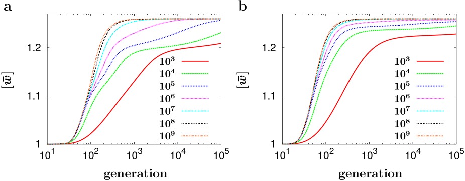
Figure 4: Mean fitness evolution in random three-locus fitness landscapes. Fitness has been averaged over $10^{4}$ realizations of the landscape and 128 population histories in each realization, with parameters $\mu=10^{-5}$ and $S=0.1$, and population sizes as indicated in the figures. Both for (a) the constrained ensemble and (b) the unconstrained ensemble the mean fitness increases monotonically with population size for all times.

In Figure 4 we show the time evolution of the mean fitness, averaged over many realizations of the landscape, for both ensembles of random three-locus landscapes; as before, all individuals are initially placed at the least fit genotype. In contrast to Figure 1, the mean fitness is now a monotonic function of population size at all times: When averaged over the landscape ensemble, there is no advantage of small populations. This however does not preclude the existence of such an advantage for individual landscapes. To test for this possibility, we introduce the probability $P(t,N,N^{\prime})$ of a small population advantage, defined as the probability that the mean fitness of a population of size $N$ at generation $t$ is larger than that of a population of size $N^{\prime}$ at the same generation, where $N<N^{\prime}$.

To determine $P(t,N,N^{\prime})$ numerically, we first calculated the mean fitness for population size $N$ by averaging over 128 independent evolutionary histories on a single landscape, and then compared it to that for a different population size $N^{\prime}$ on the same landscape. Finally the outcome of the comparison was averaged over $10^{4}$ samples of the random landscape ensemble. In order to avoid spurious contributions from cases where the fitness is in fact independent of population size and an apparent advantage of small populations arises due to fluctuations, we count only instances in which the inequality $(1-\alpha)w(N)>w(N^{\prime})$ is satisfied, where $w(N)$ stands for the calculated mean fitness for population size $N$. We choose $\alpha=10^{-3}$, which is large enough to remove the error due to fluctuations. Of course, this may also screen out landscapes with very small advantage, but we do not think that this effect is substantial, since a mean fitness advantage of less than 0.1% is negligible compared to the scale $S=0.1$ of typical selection coefficients.

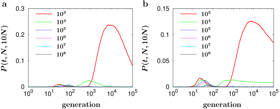
Figure 5: Probability of small population advantage in random three-locus fitness landscapes. Plots show $P(t,N,N^{\prime})$ as a function of $t$, with $N^{\prime}=10N$ and $N$ as indicated in the figures, $\mu=10^{-5}$, and $S=0.1$. Part (a) shows the constrained ensemble, part (b) the unconstrained ensembles. The constrained ensemble with the maximum fitness at the antipodal point is more likely to allow small populations to have larger mean fitness.

The resulting probabilities for the two ensembles are summarized in Figure 5. Referring first to the constrained ensemble, which mimics most closely the overall topography of the landscape equation (1), we see that a conspicuous probability for an advantage of small populations begins to appear around $10^{3}$ generations and is most pronounced for population size $N\approx 10^{3}$. Note that in Fig. 1 a where the selection coefficient is of the order of 0.1 as in Fig. 5, the fitness advantage of a small population becomes conspicuous when the population with size $10^{3}$ is compared to that with $10^{4}$ in the time window between $10^{3}$ and $10^{5}$. That is, the quantitative as well as the qualitative behavior of the house-of-cards model in the constrained ensemble is similar to the three-locus model in the previous section. Thus, we may conclude that the landscape equation (1) is quite generic within the constrained ensemble, in the sense that between 20% and 30% of all landscapes show similar dynamical features. In the unconstrained ensemble the probabilities are reduced by about a factor of 2, but the overall behavior is the same.

More than three loci

Within the house-of-cards models, it is straightforward to investigate the effect of varying the number of loci $L$. In the simulations reported in this subsection we allow for at most one mutation per individual and generation, and specify the genome-wide mutation probability $U$ rather than the mutation probability $\mu$ per locus. The general relation between $U$ and $\mu$ is (Park and Krug, 2008) $U=1-(1-\mu)^{L}\approx\mu L$ when $\mu L\ll 1$. With increasing $L$ the difference between the constrained and unconstrained ensembles becomes less important, because populations typically do not reach the global maximum within the simulation time, and hence its precise location is irrelevant. In the following we therefore restrict the discussion to the standard (unconstrained) model.

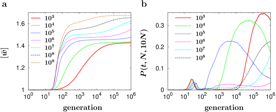
Figure 6: (a) Mean fitness evolution and (b) probability of small population advantage for the unconstrained ensemble with $L=20$ loci. Parameters are $U=10^{-5}$ and $S=0.1$, and population sizes as indicated in the figures.

As an illustration, we present simulation results for $L=20$ in Figure 6. In this case the expected fitness value of the global maximum is $\approx 2.44$ which is far larger than the mean fitness of the population with size $10^{9}$ within the observation time. This means that most of evolutions up to size $10^{9}$ and generation $10^{6}$ have not arrived at the global maximum, but rather explore the surroundings of the low fitness starting genotype. As in the three-locus case, the mean fitness averaged over all landscapes is monotonic in the population size (Figure 6a), and the plot of $P(t,N,N^{\prime})$ in Figure 6b displays a similar, though more pronounced advantage of small populations for $N=10^{3}-10^{5}$. However, for $N\geq 10^{7}$ a new peak is seen to appear in $P(t,N,N^{\prime})$ at later time, which is not present for $L=3$.

We may interpret this behavior in terms of the different evolutionary regimes described by Jain and Krug (2007b). The disappearance of the first peak in $P(t,N,N^{\prime})$ marks the point where the mutation supply rate $NU$ is sufficiently large for the population to easily escape from local fitness maxima by the creation of double mutants. Such a population will however still have difficulties to cross wider fitness valleys, and hence it will tend to get trapped at local maxima which are separated by three or more mutational steps. The mechanism for an advantage of small populations that was found in the three-locus model thus reemerges on a larger scale, giving rise to secondary peaks in $P(t,N,N^{\prime})$.

Discussion

Understanding the effect of population size on the rate of adaptation is a central problem in evolutionary theory, which continues to attract considerable attention (Weinreich and Chao, 2005; Gokhale et al., 2009; Weissman et al., 2009; Lynch and Abegg, 2010). Motivated by the experiments of Rozen et al. (2008), the present work has addressed a specific aspect of this general problem. In the experiments, several populations of E. coli consisting of either $5\times 10^{5}$ or $2.5\times 10^{7}$ individuals were evolved in a complex nutrient medium which can be modeled by a complex fitness landscape. The fitness measurements after $500$ generations showed that small populations can achieve higher fitness than large populations.

A classic scenario in which a small population can acquire an evolutionary advantage because of genetic drift has been put forward in the framework of Wright’s shifting balance theory (Wright, 1931), referred to as SBT in the following discussion. Apart from the intrinsic shortcomings of the SBT (Coyne et al., 1997), however, there are several reasons why it cannot be directly applied to the experimental situation of Rozen et al. (2008). First of all, the population in the experiments is not structured, and it is therefore not possible for different demes to occupy separate fitness peaks as assumed in phase II of the SBT. Second, the number of generations in the experiment is too small for the entire population to cross a fitness valley either by the fixation of deleterious mutations (phase I of the SBT) or by the simultaneous fixation of individually deleterious but jointly beneficial mutations (Weinreich and Chao, 2005). Hence for a proper explanation of the experimental observations it cannot be assumed that the population resides at a local fitness optimum from the beginning of the process. Rather, the evolutionary trajectories begin in a fitness valley, and the dynamics is determined by the competition between different fitness peaks that are available to the population (Rozen et al., 2008).

In the preceding sections we have demonstrated that under these conditions, small populations may indeed reach higher fitness levels than large ones because they are more likely to evade trapping at local fitness maxima. Our detailed study of a three-locus model where a single local fitness peak competes with the global maximum has shown that the dynamical behavior of the population fitness is not determined by the time scale to acquire beneficial mutation(s) alone and depends on the path probability $P_{r}(N)$ also. This probability increases from a constant value $1/3$ to $P_{r}^{SSWM}$ and finally approaches the deterministic value unity as the population size $N$ increases. For the parameter regimes in which $P_{r}$ is constant in $N$, as the waiting times $T_{\mathrm{rugged}}$ and $T_{\mathrm{smooth}}$ both decrease with $N$, larger populations are at an advantage.

However when the probability to take a rugged path increases with $N$, a larger population may get trapped at the local fitness maximum thus acquiring lower fitness than a small population. For the parameters in Figure 1, the path probability exceeds the SSWM value $0.55$ for $N>500$. From equation (18), it is approximately $0.6$ for $N=10^{3}$ but close to unity for $N\geq 10^{4}$ and therefore a population of size $N\sim 10^{3}$ is able to acquire a higher fitness than larger populations.

A key result of our analysis is that the regime of population sizes in which this mechanism operates coincides with the onset of clonal interference, which occurs precisely when the criterion in equation (20) is satisfied (Gerrish and Lenski, 1998; de Visser et al., 1999; Wilke, 2004; Park and Krug, 2007). In the context of the three-allele model discussed previously, clonal interference implies that a high fitness clone (allele C) may arise while the low fitness mutant (allele B) is still on the way to fixation, thus enhancing the probability for C to fix and increasing the probability for the population to evolve along a rugged path. From the criterion in equation (20), we can determine the mutation probability for the bacterial populations used in the experiment of Rozen et al. (2008). Since the small population advantage is observed around $N=5\times 10^{5}$ and the characteristic size of selection coefficients derived from the fitness trajectories in the experiment is $\simeq 0.1$, the estimated mutation probability is

$$\mu\approx\frac{1}{N\ln(Ns)}\simeq 10^{-6},$$ (22)

which should be interpreted as a beneficial mutation rate. This estimate is consistent with values for the beneficial mutation rate in E.coli obtained by other experimental approaches, which range from $10^{-4}$ to $10^{-7}$ (Hegreness et al., 2006; Perfeito et al., 2007).

Our theoretical analysis also shows that the advantage of small populations over large ones is transient and at sufficiently large times, the fitness of the large population exceeds that of the small population. This reversal occurs when the large population escapes the fitness valley at time $T_{\mathrm{esc}}\sim(N\mu^{2})^{-1}$ (see Eq. 7) and should be testable over an experimentally accessible time scale of $10^{3}$ generations if the population size exceeds $(10^{3}\mu^{2})^{-1}\sim 10^{9}$ where we have used (22). In the experiments of Rozen et al. (2008), the large populations had a size of $N\sim 10^{7}$ which is two orders of magnitude below our prediction and hence the reversal in the ordering of fitness was not observed. It would be interesting to test this effect in experiments using larger populations.

In their work, Rozen et al. (2008) attributed the fitness advantage seen for small populations to the heterogeneity in evolutionary trajectories. This qualitative description can be made precise by considering predictability of the first adaptive step along the evolutionary trajectory. Following Orr (2005) and Roy (2009) we define the predictability $P_{2}$ to be the probability that two replicate populations follow the same evolutionary trajectory, which equals the sum of the squares of the probability of these trajectories. Specializing to the first adaptive step in our three-locus system, the possible outcomes $\{100\}$, $\{010\}$ and $\{001\}$ occur with probability $P_{r}$, $(1-P_{r})/2$ and $(1-P_{r})/2$, respectively so that $P_{2}=P_{r}^{2}+\frac{1}{2}(1-P_{r})^{2}$ which increases from $P_{2}=1/3$ to $1$ with increasing population size, similar to the behavior of $P_{r}$ itself. For the parameter range $N\mu\ll 1,Ns\gg 1$ in which $P_{r}$ is independent of $N$, the predictability $P_{2}<1$ is also a constant and as discussed above, we do not expect a fitness advantage for such populations. Thus although small populations will exhibit heterogeneous evolutionary trajectories in general, this does not necessarily imply a fitness advantage.

The robustness of our results with respect to modifications of the fitness landscape equation (1) was addressed within the framework of two variants of the house-of-cards model. From this study we concluded that an advantage of small populations is generally not present when the mean fitness is averaged over all possible realizations of the landscape; however, in the appropriate range of time scales and population sizes identified for the landscape equation (1), a non-negligible fraction of all landscapes do display such an advantage. This agrees with the results obtained by Handel and Rozen (2009) for a class of models with tunable ruggedness, and is also consistent with the analysis of the mean fitness evolution in the infinite sites limit of the house-of-cards model by Park and Krug (2008).

Returning to the evolution experiments that initially motivated this work, we expect the effects described here to be observable whenever the underlying fitness landscape displays multiple local maxima. Among the small number of available empirical fitness landscapes, local maxima have been found in some cases (de Visser et al., 2009; Lozovsky et al., 2009) but not in others (Weinreich et al., 2006). Further work on the structure of empirical fitness landscapes is therefore needed in order to assess the generality of the proposed mechanism for an evolutionary advantage of small populations.

Acknowledgements

This work was supported by DFG within SFB 680 Molecular Basis of Evolutionary Innovations. We thank Arjan de Visser, Siegfried Roth and Sijmen Schoustra for helpful discussions and comments, and two anonymous reviewers for their suggestions on the manuscript. K.J. and J.K. acknowledge the hospitality of KITP, Santa Barbara, and support under NSF grant PHY05-51164 during the initial stages of this work.

Figures

LITERATURE CITED

- Bürger (2000) Bürger, R. 2000. The Mathematical Theory of Selection, Recombination, and Mutation. Wiley, Chichester.
- Burch and Chao (1999) Burch, C. L., and L. Chao. 1999. Evolution by small steps and rugged landscapes in the RNA virus 6. Genetics 151:921–927.
- Burch and Chao (2000) Burch, C. L., and L. Chao. 2000. Evolvability of an RNA virus is determined by its mutational neighborhood. Nature 406:625–628.
- Carneiro and Hartl (2010) Carneiro, M., and D. L. Hartl. 2010. Adaptive landscapes and protein evolution. Proc. Nat. Acad. Sci. USA 107 (suppl. 1):1747–1751.
- Coyne et al. (1997) Coyne, J. A., N. H. Barton, and M. Turelli. 1997. A critique of Sewall Wright’s shifting balance theory of evolution. Evolution 51:643–671.
- Desai and Fisher (2007) Desai, M. M., and D. S. Fisher. 2007. Beneficial mutation-selection balance and the effect of linkage on positive selection. Genetics 176:1759–1798.
- Elena and Lenski (2003) Elena, S. F., and R. E. Lenski. 2003. Evolution experiments with microorganisms: The dynamics and genetic bases of adaptation. Nature Reviews Genetics 4:457–469.
- Gerrish (2001) Gerrish, P. J. 2001. The rhythm of microbial adaptation. Nature 413:299–302.
- Gerrish and Lenski (1998) Gerrish, P. J., and R. E. Lenski. 1998. The fate of competing beneficial mutations in an asexual population. Genetica 102/103:127–144.
- Gillespie (1983) Gillespie, J. H. 1983. Some properties of finite populations experiencing strong selection and weak mutation. Am. Nat. 121:691–708.
- Gillespie (1984) ———. 1984. Molecular evolution over the mutational landscape. Evolution 38:1116–1129.
- Gokhale et al. (2009) Gokhale, C. S., Y. Iwasa, M. A. Nowak, and A. Traulsen. 2009. The pace of evolution across fitness valleys. J. Theor. Biol. 259:613–620.
- Handel and Rozen (2009) Handel, A., and D. E. Rozen. 2009. The impact of population size on the evolution of asexual microbes on smooth versus rugged fitness landscapes. BMC Evolutionary Biology 9:236.
- Hegreness et al. (2006) Hegreness, M., N. Shoresh, D. Hartl, and R. Kishony. 2006. An equivalence principle for the incorporation of favorable mutations in asexual populations. Science 311:1615–1617.
- Hermisson and Pennings (2005) Hermisson, J., and P. S. Pennings. 2005. Soft sweeps: molecular population genetics of adaptation from standing genetic variation. Genetics 169:2335–2352.
- Iwasa et al. (2004) Iwasa, Y., F. Michor, and M. A. Nowak. 2004. Stochastic tunnels in evolutionary dynamics. Genetics 166:1571–1579.
- Jain (2007) Jain, K. 2007. Evolutionary dynamics of the most populated genotype on rugged fitness landscapes. Phys. Rev. E 76:031922.
- Jain and Krug (2005) Jain, K., and J. Krug. 2005. Evolutionary trajectories in rugged fitness landscapes. J. Stat. Mech.: Theory Exp. P04008.
- Jain and Krug (2007a) ———. 2007a. Adaptation in simple and complex fitness landscapes. in U. Bastolla, M. Porto, H. E. Roman, and M. Vendruscolo, eds. Structural approaches to sequence evolution: Molecules, networks and populations. Springer, Berlin.
- Jain and Krug (2007b) ———. 2007b. Deterministic and stochastic regimes of asexual evolution on rugged fitness landscapes. Genetics 175:1275–1288.
- Kauffman and Levin (1987) Kauffman, S., and S. Levin. 1987. Towards a general theory of adaptive walks on rugged landscapes. J. Theor. Biol. 128:11–45.
- Kimura (1962) Kimura, M. 1962. On the probability of fixation of mutant genes in a population. Genetics 47:713–719.
- Kingman (1978) Kingman, J. F. C. 1978. A simple model for the balance between selection and mutation. J. Appl. Prob. 15:1–12.
- Klözer (2008) Klözer, A. 2008. NK fitness landscapes. Master’s thesis, University of Cologne, Institute for Theoretical Physics.
- Korona et al. (1994) Korona, R., C. H. Nakatsu, L. J. Forney, and R. E. Lenski. 1994. Evidence for multiple adaptive peaks from populations of bacteria evolving in a structured habitat. Proc. Nat. Acad. Sci. USA 91:9037–9041.
- Lenski and Travisano (1994) Lenski, R. E., and M. Travisano. 1994. Dynamics of adaptation and diversification: a 10,000-generation experiment with bacterial populations. Proc. Nat. Acad. Sci. USA 91:6808–6814.
- Lynch and Abegg (2010) Lynch, M., and A. Abegg. 2010. The rate of establishment of complex adaptations. Mol. Biol. Evol. 27:1404–1414.
- Lozovsky et al. (2009) Lozovsky, E. R., T. Chookajorn, K. M. Brown, M. Imwong, P. J. Shaw, S. Kamchonwongpaisan, D. E. Neafsey, D. M. Weinreich, and D. L. Hartl. 2009. Stepwise acquisition of pyrimethamine resistance in the malaria parasite. Proc. Nat. Acad. Sci. USA 106:12025–12030.
- Maynard Smith (1971) Maynard Smith, J. 1971. What use is sex? J. theor. Biol. 30:319–335.
- Miller et al. (2011) Miller, C. R., P. Joyce, and H.A. Wichman. 2011. Mutational effects and population dynamics during viral adaptation challenge current models. Genetics 187:185–202,.
- Orr (2002) Orr, H. A. 2002. The population genetics of adaptation: The adaptation of DNA sequences. Evolution 56:1317–1330.
- Orr (2005) ———. 2005. The probability of parallel evolution. Evolution 59:216–220.
- Park and Krug (2007) Park, S.-C., and J. Krug. 2007. Clonal interference in large populations. Proc. Nat. Acad. Sci. USA 104:18135–18140.
- Park and Krug (2008) ———. 2008. Evolution in random fitness landscapes: the infinite sites model. J. Stat. Mech.: Theory Exp. P04014.
- Park et al. (2010) Park, S.-C., D. Simon, and J. Krug. 2010. The speed of evolution in large asexual populations. J. Stat. Phys. 138:381–410.
- Perfeito et al. (2007) Perfeito, L., L. Fernandes, C. Mota, and I. Gordo. 2007. Adaptive mutations in bacteria: high rate and small effects. Science 317:813–815.
- Poelwijk et al. (2007) Poelwijk, F. J., D. J. Kiviet, D. M. Weinreich, and S. J. Tans. 2007. Empirical fitness landscapes reveal accessible evolutionary paths. Nature 445:383–386.
- Poelwijk et al. (2011) Poelwijk, F. J., S. Tănase-Nicola, D. J. Kiviet, S. J. Tans. 2011. Reciprocal sign epistasis is a necessary condition for multi-peaked fitness landscapes. J. Theor. Biol. 272:141–144.
- Roy (2009) Roy, S. 2009. Probing evolutionary repeatability: Neutral and double changes and the predictability of evolutionary adaptation. PLoS ONE 4:e4500.
- Rozen et al. (2008) Rozen, D. E., M. G. J. L. Habets, A. Handel, and J. A. G. M. de Visser. 2008. Heterogeneous adaptive trajectories of small populations on complex fitness landscapes. PLoS ONE 3:e1715.
- de Visser et al. (2009) de Visser, J. A. G. M., S.-C. Park, and J. Krug. 2009. Exploring the effect of sex on empirical fitness landscapes. Am. Nat. 174:S15–S30.
- de Visser et al. (1999) de Visser, J. A. G. M., C. W. Zeyl, P. J. Gerrish, J. L. Blanchard, and R. E. Lenski. 1999. Diminishing returns from mutation supply rate in asexual populations. Science 283:404–406.
- Weinreich and Chao (2005) Weinreich, D. M., and L. Chao. 2005. Rapid evolutionary escape by large populations from local fitness peaks is likely in nature. Evolution 59:1175–1182.
- Weinreich et al. (2006) Weinreich, D. M., N. F. Delaney, M. A. DePristo, and D. L. Hartl. 2006. Darwinian evolution can follow only very few mutational paths to fitter proteins. Science 312:111–114.
- Weinreich et al. (2005) Weinreich, D. M., R. A. Watson, and L. Chao. 2005. Sign epistasis and genetic constraint on evolutionary trajectories. Evolution 59:1165–1174.
- Weissman et al. (2009) Weissman, D. B., M. M. Desai, D. S. Fisher, and M. W. Feldman. 2009. The rate at which asexual populations cross fitness valleys. Theor. Pop. Biol. 75:286–300.
- Wilke (2004) Wilke, C. O. 2004. The speed of adaptation in large asexual populations. Genetics 167:2045–2053.
- Wright (1931) Wright, S. 1931. Evolution in Mendelian populations. Genetics 16:97–159.