The Next-to-Leading Order Corrections to Top Quark Decays to Heavy Quarkonia

Abstract

The decay widths of top quark to S-wave $b\bar{c}$ and $b\bar{b}$ bound states are evaluated at the next-to-leading(NLO) accuracy in strong interaction. Numerical calculation shows that the NLO corrections to these processes are remarkable. The quantum chromodynamics(QCD) renormalization scale dependence of the results is obviously depressed, and hence the uncertainties lying in the leading order calculation are reduced.

PACS number(s): 13.85.Ni, 14.40.Lb, 12.39.Hg, 12.38.Bx.

I Introduction

Since predicted by the Standard Model (SM)top3 ; top4 ; top5 , top quark has become an important role in high energy physics due to its large mass, which is close to the electroweak symmetry breaking scale top1 . A great deal of researches focusing on top quark physics have been performed after its discovery in 1995 in the Fermilab top6 . On the experiment aspect, with the running of the Tevatron and forthcoming LHC, the lack of adequate events will not be an obstacle for the top quark physics study. According to Ref. top2 , at the LHC $10^{7}\sim 10^{8}$ $t\bar{t}$ pairs can be obtained per year, so this enables people to measure various top quark decay channels. Meanwhile, the copious production of the top quarks supplies also a great number of bottom quark mesons since the dominant top quark decay channel is $t\rightarrow b+W^{+}$. Therefore, the bottom quark meson production in top quark decays may stand as an important and independent means for the study of heavy meson physics and the test of perturbative QCD (pQCD).

As the known heaviest mesons, bottomonia and $B_{c}$ ($b\bar{c}$ or $\bar{b}c$) possess particular meaning in the study of heavy flavor physics. The LHCb as a detector specifically for the heavy flavor study at the LHC will supply copious $B_{c}$ and $\Upsilon$ data for this aim. Theoretically, the direct hadroproduction of $B_{c}$ and $\Upsilon$ was studied in the literature Bc1 ; Bc7 ; Bs7 . In addition to the “direct” production, “indirect” process as in top quark decays may stand as an independent and important source for $B_{c}$ and $\Upsilon$ production. Since the top quark’s lifetime is too short to form a bound state top7 , the $B_{c}$ and $\Upsilon$ production involved scheme in top quark decays is less affected by the non-pertubative effects than in other processes. In Ref. Bc2 , the top quark decays into $\Upsilon$ and ${\bar{B}_{c}}^{*}$ at the Born level was evaluated. Recently, the S- and P-wave $B_{c}$ meson productions in top quark decays were fully evaluated, including the color-octet contributions, at the leading order accuracy of QCD by Chang $et$ $al.$ Bc3 .

Considering the importance of investigating $B_{c}$ and $\Upsilon$ in the study of perturbative Quantum Chromodynamics (pQCD) and potential model, it is reasonable and interesting to evaluate the production rates of these mesons in top quark decays at the next-to-leading order (NLO) accuracy of pQCD. At the bottom quark and charm quark mass scales the strong coupling is not very small, therefore the higher order corrections are usually large. On the other hand, in the processes of top quark decays into $\bar{B}_{c}(\Upsilon)$, the $t\rightarrow b\overline{c}(\bar{b})+c(b)+W^{+}$, there exist large scale uncertainties in the tree level calculation Bc4 . The NLO corrections should in principle minimize it and give a more precise prediction. To calculate the $\bar{B}_{c}$ and $\Upsilon$ production rates in top quark decays at the NLO accuracy are the aims of this work. In our calculation, both of the S-wave spin-singlet and -triplet states are taken into account, i.e., ${\bar{B}_{c}}^{*}$, $\bar{B}_{c}$, $\Upsilon$ and $\eta_{b}$. To deal with the non-perturbative effects, the non-relativistic QCD (NRQCD) Bc5 effective theory is employed. The calculation will be performed at the NLO in pQCD expansion, but at leading order in relativistic expansion, that is in the expansion of $v$, the relativistic velocity of heavy quarks inside bound states.

The paper is organized as follows: after the Introduction, in section II we explain the calculation of leading order decay width. In section III, virtual and real QCD corrections to Born level result are evaluated. In section IV, the numerical calculation for concerned processes at NLO accuracy of pQCD is performed, and the scale dependence of the results is shown. The last section is remained for a brief summary and conclusions.

II Calculation of The Born Level Decay Width

At the leading order in $\alpha_{s}$, there are two Feynman Diagrams for each meson production, which are shown in Figure 1. For the convenience of analytical calculation, taking $\bar{B}_{c}$ as an example, the momentum of each particle is assigned as: $p_{1}=p_{t}$, $p_{3}=p_{b}$, $p_{4}=p_{\overline{c}}$, $p_{5}=p_{c}$, $p_{6}=p_{W^{+}}$, $p_{0}=p_{3}+p_{4}$, $p_{3}=\frac{m_{b}}{m_{c}}p_{4}$. For bottomonium, the only difference is that $p_{4}$ and $p_{5}$ represent the momenta of anti-bottom quark and bottom quark which are produced in gluon splitting.

Of the $\bar{B}_{c}$ and $\bar{B}_{c}^{*}$ production in top quark decays, i.e.

$$t(p_{1})\rightarrow\bar{B}_{c}/{\bar{B}_{c}}^{*}(p_{0})+c(p_{5})+W^{+}(p_{6})\;,$$ (1)

we employ the following commonly used projection operators for quarks hadronization:

$$v(p_{4})\,\overline{u}(p_{3}) \longrightarrow {1\over 2\sqrt{2}}i\gamma_{5}(\not\!p_{0}+m_{b}+m_{c})\,\times\left({1\over\sqrt{\frac{m_{b}+m_{c}}{2}}}\psi_{\bar{B}_{c}}(0)\right)\otimes\left({{\bf 1}_{c}\over\sqrt{N_{c}}}\right)$$ (2)

and

$$v(p_{4})\,\overline{u}(p_{3}) \longrightarrow {1\over 2\sqrt{2}}\not\!\epsilon_{{\bar{B}_{c}}^{*}}(\not\!p_{0}+m_{b}+m_{c})\,\times\left({1\over\sqrt{\frac{m_{b}+m_{c}}{2}}}\psi_{{\bar{B}_{c}}^{*}}(0)\right)\otimes\left({{\bf 1}_{c}\over\sqrt{N_{c}}}\right)\,.$$ (3)

Here, $\varepsilon_{{\bar{B}_{c}}^{*}}$ is the polarization vector of ${\bar{B}_{c}}^{*}$ with $p_{0}\cdot\varepsilon=0$, ${\bf 1}_{c}$ stands for the unit color matrix, and $N_{c}=3$ for QCD. The nonperturbative parameters $\psi_{\bar{B}_{c}}(0)$ and $\psi_{{\bar{B}_{c}}^{*}}(0)$ are the Schrödinger wave functions at the origin of $b\bar{c}$ bound states, and in the non-relativistic limit $\psi_{\bar{B}_{c}}(0)=\psi_{{\bar{B}_{c}}^{*}}(0)$. In our calculation, the non-relativistic relation $m_{\bar{B}_{c}}=m_{\bar{B}_{c}^{*}}=m_{b}+m_{c}$ is also adopted.

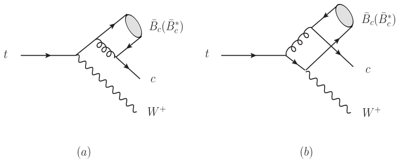
Figure 1: The leading order Feynman diagrams for $\bar{B}_{c}$ and $\bar{B}_{c}^{*}$ production in top quark decays.

The LO amplitudes for $\bar{B}_{c}$ production can then be readily obtained with above preparations. They are:

$${\cal M}_{a}=\frac{\pi\alpha_{s}g\psi_{\bar{B}_{c}}(0)V_{tb}C_{F}\delta_{j,k}}{\sqrt{6m_{\bar{B}_{c}}}}\bar{u}(p_{5})\gamma^{\mu}i\gamma_{5}(\not\!p_{0}+m_{\bar{B}_{c}})\gamma_{\mu}\frac{(\not\!p_{0}+\not\!p_{5}+m_{b})}{(p_{0}+p_{5})^{2}-m_{b}^{2}}\frac{\not\!\epsilon(p_{6})(1-\gamma_{5})}{({p_{4}+p_{5}})^{2}}u(p_{1})\;,$$ (4)

and

$${\cal M}_{b}=\frac{\pi\alpha_{s}g\psi_{\bar{B}_{c}}(0)V_{tb}C_{F}\delta_{j,k}}{\sqrt{6m_{\bar{B}_{c}}}}\bar{u}(p_{5})\gamma^{\mu}i\gamma_{5}(\not\!p_{0}+m_{\bar{B}_{c}})\frac{\not\!\epsilon(p_{6})(1-\gamma_{5})}{({p_{4}+p_{5}})^{2}}\frac{(\not\!p_{3}+\not\!p_{6}+m_{t})}{(p_{3}+p_{6})^{2}-m_{t}^{2}}\gamma_{\mu}u(p_{1})\;.$$ (5)

Here, $j$, $k$ are color indices, $C_{F}=4/3$ belongs to the $SU(3)$ color structure. For ${\bar{B}_{c}}^{*}$ production, the amplitudes can be obtained by simply substituting $i\gamma_{5}(\not\!\!p_{0}+m_{\bar{B}_{c}})$ with $\not\!\epsilon_{{\bar{B}_{c}}^{*}}(\not\!p_{0}+m_{b}+m_{c})$ in above expressions.

The Born amplitude of the processes shown in Fig.1 is then ${\cal M}_{Born}={\cal M}_{a}+{\cal M}_{b}$, and subsequently, the decay width at leading order reads:

$$\mathrm{d}\Gamma_{Born}=\frac{1}{2m_{t}}\frac{1}{2}\frac{1}{N_{c}}\sum|{\cal M}_{Born}|^{2}\mathrm{d}\textmd{PS}_{3}\;.$$ (6)

Here, $\sum$ represents the sum over polarizations and colors of the initial and final particles, $\frac{1}{2}$ and $\frac{1}{N_{c}}$ come from spin and color average of initial t quark, $\mathrm{d}\textmd{PS}_{3}$ stands for the integrants of three-body phase space, whose concrete form is

$$\mathrm{d}\textmd{PS}_{3}=\frac{1}{32\pi^{3}}\frac{1}{4m_{t}^{2}}\mathrm{d}s_{1}\mathrm{d}s_{2}\;,$$ (7)

where $s_{1}=(p_{0}+p_{5})^{2}=(p_{1}-p_{6})^{2}$ and $s_{2}=(p_{5}+p_{6})^{2}=(p_{1}-p_{0})^{2}$ are Mandelstam variables. The upper and lower bounds of the above integration are

$$s_{1}^{max}= \frac{\sqrt{f[m_{t}^{2},s_{2},m_{\bar{B}_{c}}^{2}]\cdot f[s_{2},m_{c}^{2},m^{2}_{W}]}+[m_{t}^{2}-s_{2}-(m_{b}+m_{c})^{2}](s_{2}+m_{c}^{2}-m^{2}_{W})}{2s_{2}}$$ (8)

$$+m_{\bar{B}_{c}}^{2}+m_{c}^{2}\;,$$

$$s_{1}^{min}= -\frac{\sqrt{f[m_{t}^{2},s_{2},m_{\bar{B}_{c}}^{2}]\cdot f[s_{2},m_{c}^{2},m^{2}_{W}]}-[m_{t}^{2}-s_{2}-(m_{b}+m_{c})^{2}](s_{2}+m_{c}^{2}-m^{2}_{W})}{2s_{2}}$$ (9)

$$+m_{\bar{B}_{c}}^{2}+m_{c}^{2}$$

and

$$s_{2}^{max}=[m_{t}-(m_{b}+m_{c})]^{2}\;,\;s_{2}^{min}=(m_{c}+m_{W})^{2}$$ (10)

with

$$f[x,y,z] = (x-y-z)^{2}-4yz\;.$$ (11)

III The Next-to-Leading Order Corrections

At the next-to-leading order, the top quark decays to $\bar{B}_{c}$ and $\Upsilon$ include the virtual and real QCD corrections to the leading order process, as shown in Figs.2-5. With virtual corrections, the decay widths at the NLO can be formulated as

$$\mathrm{d}\Gamma_{Virtual}=\frac{1}{2m_{t}}\frac{1}{2}\frac{1}{N_{c}}\sum 2\textmd{Re}({\cal M}_{Born}^{*}{\cal M}_{Virtual})\mathrm{d}\textmd{PS}_{3}\;.$$ (12)

The ultraviolet(UV) and infrared(IR) divergences usually exist in virtual corrections. We use the dimensional regularization scheme to regularize the UV and IR divergences, similar as performed in Ref.Bc6 , and the Coulomb divergence is regularized by the relative velocity $v$. In dimensional regularization, $\gamma_{5}$ is difficult to deal with. In this calculation, we adopt the Naive scheme, that is, $\gamma_{5}$ anticommutates with each $\gamma^{\mu}$ matrix in d-dimension space-time, $\{\gamma_{5},\gamma^{\mu}\}=0$. The UV divergences exist merely in self-energy and triangle diagrams, which can be renormalized by counter terms. The renormalization constants include $Z_{2}$, $Z_{3}$, $Z_{m}$, and $Z_{g}$, corresponding to quark field, gluon field, quark mass, and strong coupling constant $\alpha_{s}$, respectively. Here, in our calculation the $Z_{g}$ is defined in the modified-minimal-subtraction ($\mathrm{\overline{MS}}$) scheme, while for the other three the on-shell ($\mathrm{OS}$) scheme is adopted, which tells

$$\delta Z_{m}^{OS}=-3C_{F}\frac{\alpha_{s}}{4\pi}\left[\frac{1}{\epsilon_{UV}}-\gamma_{E}+\ln\frac{4\pi\mu^{2}}{m^{2}}+\frac{4}{3}+{\mathcal{O}}(\epsilon)\right]\;,$$

$$\delta Z_{2}^{OS}=-C_{F}\frac{\alpha_{s}}{4\pi}\left[\frac{1}{\epsilon_{UV}}+\frac{2}{\epsilon_{IR}}-3\gamma_{E}+3\ln\frac{4\pi\mu^{2}}{m^{2}}+4+{\mathcal{O}}(\epsilon)\right]\;,$$

$$\delta Z_{3}^{OS}=\frac{\alpha_{s}}{4\pi}\left[(\beta_{0}-2C_{A})(\frac{1}{\epsilon_{UV}}-\frac{1}{\epsilon_{IR}})+{\mathcal{O}}(\epsilon)\right]\;,$$

$$\delta Z_{g}^{\overline{MS}}=-\frac{\beta_{0}}{2}\frac{\alpha_{s}}{4\pi}\left[\frac{1}{\epsilon_{UV}}-\gamma_{E}+\ln 4\pi+{\mathcal{O}}(\epsilon)\right]\;.$$ (13)

Here, $\beta_{0}=(11/3)C_{A}-(4/3)T_{f}n_{f}$ is the one-loop coefficient of the QCD beta function; $n_{f}=5$ is the number of active quarks in our calculation; $C_{A}=3$ and $T_{F}=1/2$ attribute to the SU(3) group; $\mu$ is the renormalization scale.

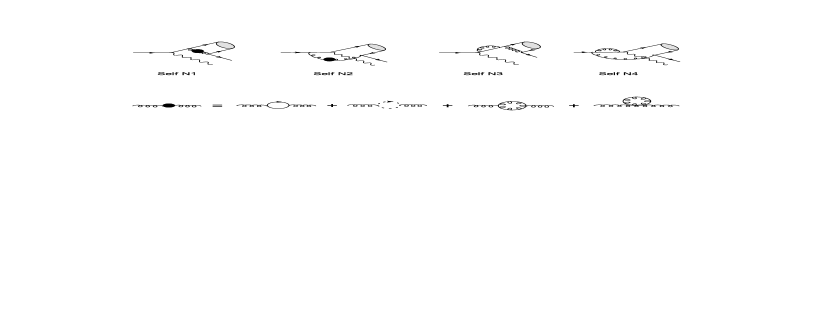
Figure 2: The self-energy diagrams in virtual corrections.

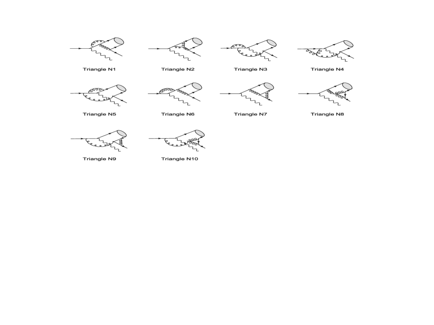
Figure 3: The triangle diagrams in virtual corrections.

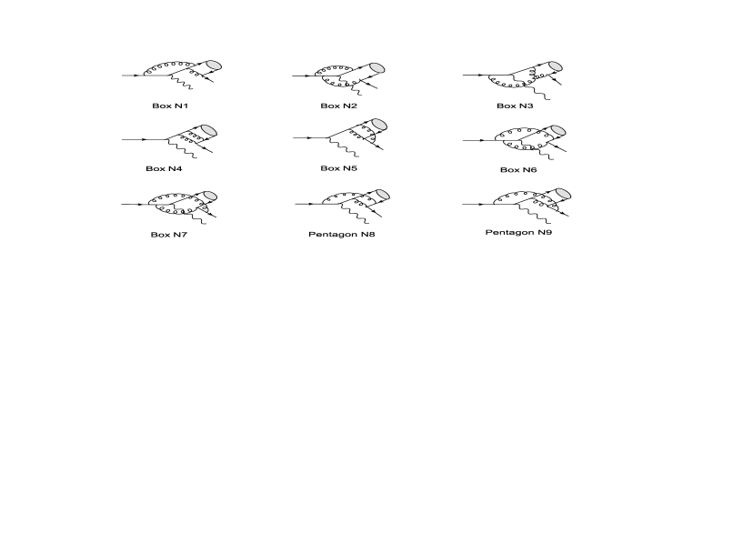
Figure 4: The box and pentagon diagrams in virtual corrections.

In virtual corrections, IR divergences remain in the triangle and box diagrams. Of all the triangle diagrams, only two have IR divergences, which are denoted as $\mathrm{TriangleN7}$ and $\mathrm{TriangleN9}$ in Fig.3. Of the diagrams in Fig.4, $\mathrm{BoxN3}$ has no IR singularity, while $\mathrm{BoxN4}$ and $\mathrm{PentagonN9}$ have Coulomb singularities and $\mathrm{PentagonN9}$ possesses ordinary IR singularity as well. The remaining diagrams all have IR singularities, while the combinations $\mathrm{BoxN2+BoxN6}$, $\mathrm{BoxN1+PentagonN8+TriangleN9}$, $\mathrm{BoxN5+TriangleN7}$ are IR finite. The Coulomb singularities belonging to $\mathrm{BoxN4}$ and $\mathrm{PentagonN9}$ can be regularized by the relative velocity $v$. After regularization procedure, the $\frac{1}{\epsilon}$ term will be canceled out by the counter terms of external quarks which form the $\bar{B}_{c}$ or $\Upsilon$, while the $\frac{1}{v}$ term will be mapped onto the wave functions of the concerned heavy mesons. The remaining IR singularities in $\mathrm{BoxN7}$ and $\mathrm{BoxN9}$ are canceled by the corresponding parts in real corrections. In the end, the IR and Coulomb divergences in virtual corrections can be expressed as

$$\mathrm{d}\Gamma_{virtual}^{IR,Coulomb}=\mathrm{d}\Gamma_{Born}\frac{4\alpha_{s}}{3\pi}\left[\frac{\pi^{2}}{v}-\frac{1}{\epsilon}-\frac{p_{t}\cdot p_{c}x_{s}\ln x_{s}}{m_{c}m_{t}(1-x_{s}^{2})}\frac{1}{\epsilon}\right]\;,$$ (14)

with $p_{t}=p_{1}$, $p_{c}=p_{5}$ and $x_{s}=\frac{1-\sqrt{1-2m_{c}m_{t}/(m_{c}m_{t}-p_{t}\cdot p_{c})}}{1+\sqrt{1-2m_{c}m_{t}/(m_{c}m_{t}-p_{t}\cdot p_{c})}}$. Here, in this work $\frac{1}{\epsilon}$ in fact represents $\frac{1}{\epsilon}-\gamma_{E}+\ln(4\pi\mu^{2})$.

Figure 5: The real correction Feynman diagrams that contribute to the production of $\bar{B}_{c}$ or $\bar{B}_{c}^{*}$.

Of our concerned processes, there are $12$ different diagrams in real correction, as shown in Fig.5. Among them, $\mathrm{RealN2}$, $\mathrm{RealN3}$, $\mathrm{RealN8}$, and $\mathrm{RealN9}$ are IR-finite, meanwhile the combinations of $\mathrm{RealN1+RealN5}$ and $\mathrm{RealN10+RealN11}$ exibit no IR singularities as well, due to the reasons of gluon connecting to the $b$ or $\bar{c}$ quark of final $\bar{B}_{c}$ or $\Upsilon$. The remaining diagrams, $\mathrm{RealN4}$, $\mathrm{RealN6}$, $\mathrm{RealN7}$, and $\mathrm{RealN12}$ are not IR singularity free. To regularize the IR divergence, we enforce a cut on the gluon momentum, the $p_{7}$. The gluon with energy $p_{7}^{0}<\delta$ is considered to be soft, while $p_{7}^{0}>\delta$ is thought to be hard. The $\delta$ is a small quantity with energy-momentum unit. In this case, the IR term of the decay width can then be written as:

$$\mathrm{d}\Gamma_{Real}^{IR}=\frac{1}{2m_{t}}\frac{1}{2}\frac{1}{N_{c}}\sum|{\cal M}_{Real}|^{2}\;\mathrm{d}\textmd{PS}_{4}\mid_{soft}\;,$$ (15)

where $\mathrm{d}\textmd{PS}_{4}$ is the four-body phase space integrants for real correction. Under the condition of $p_{7}^{0}<\delta$, in the Eikonal approximation we obtain

$$\mathrm{d}\textmd{PS}_{4}\mid_{soft}=\mathrm{d}\textmd{PS}_{3}\frac{d^{3}p_{7}}{(2\pi)^{3}2p_{7}^{0}}\mid_{p_{7}^{0}<\delta}\;$$ (16)

In the small $\delta$ limit, the IR divergent terms in real correction can therefore be expressed as

$$\mathrm{d}\Gamma_{Real}^{IR}=\mathrm{d}\Gamma_{Born}\frac{4\alpha_{s}}{3\pi}\left\{\left(\frac{1}{\epsilon}-\textmd{Log}(\delta^{2})\right)\left[1+\frac{p_{t}\cdot p_{c}x_{s}\ln x_{s}}{m_{c}m_{t}(1-x_{s}^{2})}\right]+\rm{finite\;terms}\right\}\;.$$ (17)

Here, the $\textmd{Log}(\delta^{2})$ involved terms will be canceled out by the $\delta$-dependent terms in the hard sector of real corrections. Referring to the Eq.(14), it is obvious that the IR divergent terms in real and virtual corrections cancel with each other. In case of hard gluons in real correction, the decay width reads

$$\mathrm{d}\Gamma_{Real}^{hard}=\frac{1}{2m_{t}}\frac{1}{2}\frac{1}{N_{c}}\sum|{\cal M}_{Real}|^{2}\;\mathrm{d}\textmd{PS}_{4}\mid_{hard}\;.$$ (18)

In this case the phase space $\mathrm{d}\textmd{PS}_{4}\mid_{hard}$ can be written as

$$\mathrm{d}\textmd{PS}_{4}\mid_{hard}=\frac{2}{(4\pi)^{6}} \frac{\sqrt{(sy+m_{c}^{2}-m_{W}^{2})^{2}-4sym_{c}^{2}}}{y}\int_{{p_{0}}^{0}_{-}}^{{p_{0}}^{0}_{+}}\mathrm{d}{p_{0}}^{0}\int_{-1}^{1}\mathrm{d}\cos\theta_{c}\int_{0}^{2\pi}\mathrm{d}\phi_{c}$$ (19)

$$\times\left\{\int_{\delta}^{{p_{7}}^{0}_{-}}\mathrm{d}{p_{7}}^{0}\int_{y_{-}}^{y_{+}}\mathrm{d}y+\int_{{p_{7}}^{0}_{-}}^{{p_{7}}^{0}_{+}}\mathrm{d}{p_{7}}^{0}\int_{\frac{(m_{c}+m_{W})^{2}}{s}}^{y_{+}}\mathrm{d}y\right\}$$

with

$${p_{0}}^{0}_{-}=m_{b}+m_{c}\;,$$ (20)

$${p_{0}}^{0}_{+}=\frac{s+m_{b}^{2}-m_{W}^{2}+2m_{b}m_{c}-2m_{W}\cdot m_{c}}{2\sqrt{s}}\;,$$ (21)

$${p_{7}}^{0}_{-}=\frac{s+m_{b}^{2}-m_{W}^{2}+2m_{b}m_{c}-2m_{W}\cdot m_{c}-2\sqrt{s}{p_{0}}^{0}}{2\sqrt{s}-2{p_{0}}^{0}+2\sqrt{|\overrightarrow{{p_{0}}}|}}\;,$$ (22)

$${p_{7}}^{0}_{+}=\frac{s+m_{b}^{2}-m_{W}^{2}+2m_{b}m_{c}-2m_{W}\cdot m_{c}-2\sqrt{s}{p_{0}}^{0}}{2\sqrt{s}-2{p_{0}}^{0}-2\sqrt{|\overrightarrow{p_{0}}|}}\;,$$ (23)

$$y_{-}=\frac{1}{s}[(\sqrt{s}-{p_{0}}^{0}-{p_{7}}^{0})^{2}-|\overrightarrow{{p_{0}}}|^{2}-({p_{7}}^{0})^{2}-2|\overrightarrow{p_{0}}|p_{7}^{0}]\;,$$ (24)

$$y_{+}=\frac{1}{s}[(\sqrt{s}-{p_{0}}^{0}-{p_{7}}^{0})^{2}-|\overrightarrow{{p_{0}}}|^{2}-({p_{7}}^{0})^{2}+2|\overrightarrow{p_{0}}|{p_{7}}^{0}]\;,$$ (25)

where $y$ is a dimensionless parameter defined as $y=(p_{1}-p_{0}-p_{7})^{2}/s$ with $\sqrt{s}=m_{t}$, and

$$|\overrightarrow{p_{0}}|=\sqrt{({p_{0}}^{0})^{2}-m_{\bar{B}_{c}}^{2}}\;.~{}~{}~{}~{}~{}~{}~{}~{}~{}~{}~{}~{}~{}~{}~{}~{}~{}~{}~{}~{}~{}~{}~{}~{}~{}~{}~{}~{}~{}~{}~{}~{}~{}~{}~{}$$ (26)

The sum of the soft and hard sectors gives the total contribution of real corrections, i.e., $\Gamma_{Real}=\Gamma_{Real}^{IR}+\Gamma_{Real}^{hard}$.

With the real and virtual corrections, we then obtain the total decay width of $t$ quark to $\bar{B}_{c}$ and $\Upsilon$ at the NLO accuracy of QCD

$$\Gamma_{total}=\Gamma_{Born}+\Gamma_{Virtual}+\Gamma_{Real}+{\mathcal{O}}(\alpha_{s}^{4})\;.$$ (27)

In above expression, the decay width is UV and IR finite. In our calculation the FeynArts feynarts was used to generate the Feynman diagrams, the amplitudes were generated by the FeynCalc feyncalc , and the LoopTools looptools was employed to calculate the Passarino-Veltman integrations. The numerical integrations of the phase space were performed by the MATHEMATICA.

IV Numerical results

To complete the numerical calculation, the following ordinarily accepted input parameters are taken into account:

$$m_{b}=4.9\;\textmd{GeV},\;m_{c}=1.5\;\textmd{GeV},\;m_{t}=174\;\textmd{GeV},\;m_{W}=80\;\textmd{GeV}\;,$$ (28)

$$\psi_{\bar{B}_{c}}(0) = \psi_{\bar{B}_{c}^{*}}(0)=\frac{R_{1}(0)}{\sqrt{4\pi}}=0.3616\;\mathrm{GeV}^{3/2}\;,$$ (29)

$$\psi_{\Upsilon}^{LO}(0) = \psi_{\eta_{b}}^{LO}(0)=\frac{R_{2}^{LO}(0)}{\sqrt{4\pi}}=0.6812\;\mathrm{GeV}^{3/2}\;,$$ (30)

$$\psi_{\Upsilon}^{NLO}(0) = \psi_{\eta_{b}}^{NLO}(0)=\frac{R_{2}^{NLO}(0)}{\sqrt{4\pi}}=\frac{R_{2}^{LO}(0)}{\sqrt{4\pi-16C_{F}\alpha_{s}}}=0.8277\;\mathrm{GeV}^{3/2}\;,$$ (31)

$$V_{tb}=1.0,\;\;\;\;G_{F}=1.1660\times 10^{-5}\;\mathrm{GeV}^{-2}\;.$$ (32)

Here, $V_{tb}$ is the Cabibbo-Kobayashi-Maskawa(CKM) matrix element and $G_{F}$ is weak interaction Fermi constant.

In above numerical calculation inputs, the radial wave function at the origin for S-wave $\bar{B}_{c}^{*}(\bar{B}_{c})$ system is estimated by potential model Bc8 , while the corresponding $\Upsilon(\eta_{b})$ nonperturbative parameter is determined from its electronic decay rate Bc7 . One loop result of strong coupling constant is taken into account, i.e.

$$\alpha_{s}(\mu)=\frac{4\pi}{(11-\frac{2}{3}n_{f})\mathrm{Log}(\frac{\mu^{2}}{\Lambda_{QCD}^{2}})}\;.$$ (33)

With the above preparation, one can readily obtain the decay widths of top quark to $b\bar{c}$ and $b\bar{b}$ mesons, as listed in Table 1. To see the scale dependence of the LO and NLO results, the ratios $\Gamma(\mu)/\Gamma(2m_{c})$ for $b\bar{c}$ system and $\Gamma(\mu)/\Gamma(2m_{b})$ for $b\bar{b}$ system are showed in Figures 6 and 7, respectively. Calculation tells that after including the NLO corrections, the energy scale dependence of the results is reduced, as expected.

Table 1: The decay widths of the processes $t\rightarrow\bar{B}_{c}^{*}+W^{+}+c$, $t\rightarrow\bar{B}_{c}+W^{+}+c$, $t\rightarrow\Upsilon+W^{+}+b$ and $t\rightarrow\eta_{b}+W^{+}+b$ at the tree level and with the NLO QCD corrections are presented in two renormalization scale $\mu$ limits, those are $2m_{c}$ and $m_{t}$ for the first two processes and $2m_{b}$ and $m_{t}$ for the other two.

	$t\rightarrow\bar{B}_{c}^{*}+W^{+}+c$		$t\rightarrow\bar{B}_{c}+W^{+}+c$		$t\rightarrow\Upsilon+W^{+}+b$		$t\rightarrow\eta_{b}+W^{+}+b$
$\mu$	$2m_{c}$	$m_{t}$	$2m_{c}$	$m_{t}$	$2m_{b}$	$m_{t}$	$2m_{b}$	$m_{t}$
$\Gamma_{LO}$	0.793MeV	0.151MeV	0.572MeV	0.109MeV	26.8keV	9.54keV	27.1keV	9.67keV
$\Gamma_{NLO}$	0.619MeV	0.307MeV	0.514MeV	0.227MeV	52.3keV	28.2keV	34.3keV	24.5keV

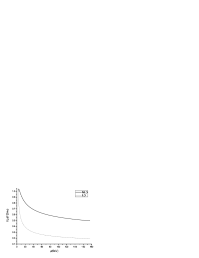
Figure 6: The ratio $\Gamma(\mu)/\Gamma(2m_{c})$ versus renormalization scale $\mu$ in $t$ quark decays. The left diagram for the $b\bar{c}$ spin-singlet state $\bar{B}_{c}$ and the right diagram for the spin-triplet state $\bar{B}_{c}^{*}$.

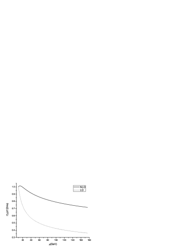
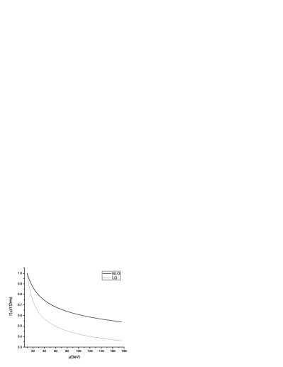
Figure 7: The ratio $\Gamma(\mu)/\Gamma(2m_{b})$ versus renormalization scale $\mu$ in $t$ quark decays. The left diagram for the $b\bar{b}$ spin-singlet state $\eta_{b}$ and the right diagram for the spin-triplet state $\Upsilon$.

V Summary and Conclusions

In this work we have calculated the decay widths of top quark to S-wave $b\bar{c}$ and $b\bar{b}$ bound states at the NLO accuracy of perturbative QCD. Considering that there will be copious $t\bar{t}$ data in the near future at the LHC, our results are helpful to the study of the indirect production of these states. They may be also useful to the future study of NLO heavy quark to $b\bar{c}$ and $b\bar{b}$ bound states fragmentation functions.

Numerical results indicate that the NLO corrections greatly enhance the LO results for $b\bar{b}$ system, while slightly decrease the $b\bar{c}$ states production widths. The main reason for this difference is that the NLO wave function for bottomonium is much larger than that of LO one, while for the calculation of $\bar{B}_{c}$ meson, the same wave function given by potential model is used. Although from Table I, superficially the number of indirectly produced $\bar{B}_{c}$ overshoots that of $\Upsilon$, experimentally to detect the latter is much easier than the former. Since top quark dominantly decays into $b$ and $W^{+}$ final state with a width of 1.5 GeV or so, numerical results remind us that the $\Upsilon$ indirect production from top quark decay is detectable, while it is hard to pin down the $\bar{B}_{c}$ states by this way.

The numerical calculation also shows that the next-to-leading order QCD corrections to processes $t\rightarrow b\bar{c}(b\bar{b})+W^{+}+c(b)$ decrease the energy scale dependence of the decay widths as expected, and hence the uncertainties in theoretical estimation. Future precise experiment on the concerned processes may provide a test on the theoretical framework for heavy quarkonium production and the reliability of perturbative calculation for them.

Acknowledgments

This work was supported in part by the National Natural Science Foundation of China(NSFC) under the grants 10935012, 10928510, 10821063 and 10775179, by the CAS Key Projects KJCX2-yw-N29 and H92A0200S2.

References

(1) W. Hollik, in Proceedings of the XVI International Symposium on
Lepton-Photon Interactions, Connell University, Ithaca, N.Y., Aug.
10-15 1993; M. Swartz, in Proceedings of the XVI International
Symposium on Lepton-Photon Interactions, Connell University, Ithaca,
N.Y., Aug. 10-15 1993.
(2) G. Altarelli, in Proceedings of Interational University School of
Nuclear and Partical Physics: Substructures of Matter as Revealed
with Electroweak Probes, Schladming, Ausria, 24 Feb - 5 Mar. 1993.
(3) G. Altarelli, CERN-TH-7319/94, talk at 1st International Conference
on Phenomenology of Unification: from Present to Future, Rome,
Itali, 23-26 Mar 1994.
(4) G. L. Kane, in Proceedings of the Workshop on High Energy Phenomenology,
Mexico City, July 1-10, 1991.
(5) F. Abe, et al. (CDF Collaboration), Phys. Rev. Lett. 74, 2626
(1995); S. Abachi, et al. (D0 Collaboration), Phys. Rev. Lett. 74,
2632 (1995).
(6) N. Kidonakis and R. Vogt, Int. J. Mod. Phys. A20, 3171, (2005); F. Hubaut,
et al., ATLAS collaboration, hep-ex/0605029;
V. Barger and R. J. Phillips, Preprint MAD/PH/789, 1993.
(7) E. Braaten and T.C. Yuan, Phys. Rev. Lett. 71, 1673 (1993); ibid, Phys.
Rev. D50, 3176 (1994); C.-H. Chang and Y.-Q. Chen, Phys. Lett. B284,
127 (1992); ibid, Phys. Rev. D46, 3845 (1992); Y.-Q. Chen, Phys.
Rev. D48, 5181 (1993); T.C. Yuan, Phys. Rev. D50, 5664 (1994).
(8) E. Braaten, K. Cheung and T.C. Yuan, Phys. Rev. D48, 4230 (1993);
ibid, Phys. Rev. D48, R5049 (1993).
(9) K. Kolodzidj, A. Leike and R. Ruckl, Phys. Lett. B355, 337 (1995);
C.-H. Chang, Y.-Q. Chen, Phys. Lett. B364, 78 (1995); C.-H. Chang,
Y.-Q. Chen, Phys. Rev. D48, 4086 (1993); C.-H. Chang, Int. J. Mod.
Phys. A21, 777 (2006); C.-H. Chang, J.-X. Wang and X.-G. Wu, Phys.
Rev. D70, 114019 (2004); C.-H. Chang, C.-F. Qiao, J. X. Wang and
X.-G. Wu, Phys. Rev. D71, 074012 (2005); C.-H. Chang, X.-G. Wu,
Eur.Phys.J.C38, 267(2004); C.-H. Chang, C. Driouichi, P. Eerola and
X.-G. Wu, Comput. Phys. Commun. 159, 192(2004); C.-H. Chang, J.-X.
Wang and X.-G. Wu, Comput. Phys. Commun. 174, 241(2006).
(10) I.I. Bigi, Yu L. Dokshitzer, V.A. Khoze, J.H. Kuhn and
P. Zerwas, Phys. Lett. B181, 157 (1986); L.H. Orr and J.L. Rosner,
Phys. Lett. B246, 221 (1990).