On the Role of Quantum Events in Double-Slit Experiments

Abstract.

We formulate the Schrödinger equation as the equation of motion of a small external influence which serves as the initial boundary condition of a physical system in classical laboratory space. The Hilbert space of possible external influences for a given physical system is then equivalent to the Hilbert space of a quantum system without spin. We discuss the double-slit experiment in the context of this approach and show that wave-particle dualism reduces to the choice of a basis in the geometrical construction of the Hilbert space of small external influences.

1. Introduction

The current development in mastering the creation of smallest objects rises a new era of tests, which challenges quantum theory on it’s most fundamental level [1]. The nature of these tests will move hypothetical Gedankenexperiments into the reach of experimental confirmation, and shine new light on the interpretation issues, which plague quantum mechanics from it’s very beginnings. As this recent progress tackles the issues at an interpretation level only, it needs to be accompanied by a structural rethinking of the theoretical fundamental concepts to gain substantially new insight.

We approach quantum mechanics by using the mathematical formalism to variational problems of Gelfand and Fomin [2], and investigate the time evolution of an external influence, which serves as the initial boundary condition of a classical physical system given with free initial point.

The necessary and sufficient condition for the external influence to serve as a boundary condition for the classical system in the entire time interval is given by the Hamilton-Jacobi equation. We use the algebraic one-to-one correspondence between the elements of the algebra of transformations and the elements of the corresponding covering group near the identity to derive the Schrödinger equation as the equation of motion of a field theory in classical configuration space for a small external influence. The Hilbert space of quantum states in energy eigenstate representation corresponds, then, to the set of possible solutions of the above field theory, where only the set of basis vectors of this solution space is observable in classical space due to the role of the Hamilton-Jacobi equation as the necessary and sufficient condition.

The distinguished role of the energy eigenvalue representation enables us to apply our formalism to the experimental results of a double-slit experiment without modification and explains the continuity of the interference pattern in a natural way. This is in contrast to standard quantum mechanics, where one needs to extend the formalism by alternative methods, e.g. the positive operator valued measure (POVM) approach [3], [4], to formulate the observed results of the double-slit experiment. Our results allow us to show in particular that the wave-particle dualism observed in the double-slit experiment reduces to the experimental realization of the choice of a basis in a degenerate Hilbert space constituted by the energy eigenfunctions emanating from each slit.

Another particular aspect in our approach is the close connection between the quantum object - the small external influence as a boundary condition - and the classical laboratory configuration - the influenced classical physical system, which emphasizes the geometry of the classical configuration space at the time of the appearance of the initial influence in the classical system. Our view shifts the quantum property, particle or wave, of a quantum object to the property of a quantum event, the event of appearance in classical laboratory space with configuration space geometry given at this point in time. This explains the observed behaviour of delayed choice experiments if we regard the contact of the quantum object with the screen/counter as the quantum event of significance.

From a formal perspective our derivation is closely related to Schrödinger’s first note [5]. But in contrast to Schrödinger, who abandoned this approach by lack of physical justification, we have an intuitive physical interpretation and mathematically rigorous derivation which gives new insight into the nature of quantum mechanics.

2. Quantum System as External Influence

Let us consider a physical system with action

(2.1)

$$\int_{a}^{b}L(t,q_{1},\ldots,q_{n},\dot{q}_{1},\ldots,\dot{q}_{n})dt+g_{1}(a,q_{1}(a),\ldots,q_{n}(a))+g_{2}(b,q_{1}(b),\ldots,q_{n}(b)).$$

and variable endpoints $a$ and $b$. The action of this system differs from the familiar action

(2.2)

$$\;\;\;\;\;\;\;\;\;\;\int_{a}^{b}L(t,q_{1},\ldots,q_{n},\dot{q}_{1},\ldots,\dot{q}_{n})dt$$

by the additional terms $g(a,q_{1}(a),\ldots,q_{n}(a))$ and $g_{2}(b,q_{1}(b),\ldots,q_{n}(b))$, which are functions of the boundary points only. As known from elementary theory these functions serve as the boundary conditions which single out a definite solution and represent the external influence on a physical system described by the Lagrangian (2). As an example, suppose the above Lagrangian (2) represents an experimental set up, which is kicked off and changes to its initial state at the free initial time $a$. Then, this Lagrangian describes the evolution of the classical physical system over time $t$ in the laboratory. For reasons which will be clear later in the text we will call the system described by (2) the laboratory system in the following.

The dynamics of the laboratory system is given by the Euler equations

(2.3) $$\frac{\partial L}{\partial q_{i}}-\frac{d}{dt}\left(\frac{\partial L}{\partial\dot{q_{i}}}\right)=0,$$

and the additional boundary conditions

(2.4) $$\left.\frac{\partial L}{\partial\dot{q_{i}}}\right|_{t=a}-\frac{\partial g_{1}(a,q)}{\partial q_{i}}=0$$

and

(2.5) $$\left.\frac{\partial L}{\partial\dot{q_{i}}}\right|_{t=b}-\frac{\partial g_{2}(b,q)}{\partial q_{i}}=0.$$

Instead of investigating the equation of motions of the laboratory system let us concentrate on the initial boundary conditions and write the external influence

(2.6) $$g_{1}(a,q)=g(t,q)\bigg{|}_{t=a}$$

as a function of time evaluated at $a$ and omit the subscript in the following. Note similar results can be observed for the boundary conditions at the terminal point, which we will ignore in the following by assuming that $g_{2}(b,q_{1}(b),\ldots,q_{n}(b))=0$ at the terminal point $b$.

Condition (2.4) relates the external initial influence $g(a,q)$ to the momentum of the laboratory system

(2.7) $$\left.p_{i}(t,q,\dot{q})\right.\bigg{|}_{t=a}=\left.\frac{\partial g(t,q)}{\partial q_{i}}\right.\bigg{|}_{t=a}$$

at the initial point $a$, where we define the momentum as usual as the velocity derivative of the Lagrangian

(2.8) $$p_{i}(t,q,\dot{q})=\frac{\partial L(t,q,\dot{q})}{\partial\dot{q_{i}}}.$$

Relations (2.7) and (2.8) allow us to rewrite the boundary conditions as functions of configuration space variables

(2.9) $$\dot{q_{i}}(a)=\varphi_{i}(q)\bigg{|}_{t=a}\ \ \ \ \ \ \ (i=1,\ldots,n),$$

which can be thought to assign a direction to every point in the hyperplane $t=a$ and allows us to define a family of boundary conditions as follows. The family of boundary conditions

(2.10) $$\dot{q_{i}}(t)=\varphi_{i}(t,q)\ \ \ \ \ \ \ (i=1,\ldots,n)$$

imposed for every $t\in[a,b]$ represents a field of the functional (2) if

• there exists a function $g(t,q)$ such that

  (2.11) $$\left.p_{i}(t,q,\varphi(q))\right.\bigg{|}_{t=a}=\left.\frac{\partial g(t,q)}{\partial q_{i}}\right.\bigg{|}_{t=a}.$$

  That is, the external influence represented by $g(t,q)$ is in contact with the laboratory system imposing the initial momentum $p_{i}(a,q(a),\dot{q}(a))$ at time $a$.

• every extremal, i.e. solution of the Euler equations, satisfying the boundary conditions

  (2.12) $$\dot{q_{i}}(t_{1})=\varphi^{(1)}_{i}(q)\bigg{|}_{t=t_{1}}$$

  also satisfies the boundary conditions

  (2.13) $$\dot{q_{i}}(t_{2})=\varphi^{(2)}_{i}(q)\bigg{|}_{t=t_{2}}$$

  at the different point in time $t_{2}$ and vice versa, i.e. the boundary conditions are traceable in time. Boundary conditions of this type are called consistent.

Thus, the influence function $g(t,q)$ acts as a kind of potential in configuration space for the family of boundary conditions. Note the potential $g(t,q)$ is given at specific points in time where the configuration space points should be regarded as a set of points at this given time and not parameterized by $t$ as (2.11) is a relation for equal times. Since boundary conditions describe the external influence of an unknown source to a physical system, which can be completely unrelated at different points in time, this means physically spoken, that we restrict our investigation to the class of external influences which are historically traceable and have a configuration space representation of fields which are derivable from a potential.

Then, the natural question arises which condition must fulfill the external influence function $g(t,q)$ to keep the ability to kick off the laboratory system described by (2) at an arbitrary point $t\in[a,b]$ in time. Gelfand and Fomin, [2] p. 146, showed that the necessary and sufficient condition, called consistency condition, is the Hamilton-Jacobi equation

(2.14) $$\frac{\partial g(t,q)}{\partial t}+H\left(t,q,\frac{\partial g(t,q)}{\partial q_{1}},\ldots,\frac{\partial g(t,q)}{\partial q_{n}}\right)=0,$$

with Hamilton function $H(t,q,p)$. Thus, the set of external influence functions $\{g_{i}\}$, which constitute the solutions of the Hamilton-Jacobi equation (2.14) in local coordinates, are the generators of the canonical transformation in the laboratory system and, therefore, the external influence function $g\in\{g_{i}\}$ is an element of a Lie algebra.

Suppose we have an external influence $g$ which causes a very small transformation in laboratory space. Then, we can use the isomorphism between elements in the neighbourhood of 0 of a Lie algebra $\mathfrak{g}$ and the Lie subgroup $G_{0}$ of elements connected to the identity established via the inverse exponential map

(2.15) $$g=\ln\psi$$

and do the ansatz

(2.16) $$g(t,q)=k\ln\psi(t,q)$$

in local coordinates. Physically spoken, this means we want to investigate the object itself represented as an element of the group of objects and are not interested in the information space generated by the external influence given by the tangential space, which is isomorphic to the Lie algebra. Then (2.14) reads

(2.17) $$\frac{k}{\psi(t,q)}\frac{\partial\psi(t,q)}{\partial t}+H\left(q,\frac{k}{\psi(t,q)}\frac{\partial\psi(t,q)}{\partial q}\right)=0,$$

where the constant $k$ is assumed to be small to guarantee the smallness of $g(t,q)$ over entire configuration space and time. In fact we know from experiment that nature has chosen a very small value

(2.18) $$k\propto\hbar$$

with Planck’s constant $\hbar$.

For conservative systems $H=E$ relation (2.17) decouples into

(2.19) $$\frac{k}{\psi(t,q)}\frac{\partial\psi(t,q)}{\partial t}+E=0$$

and

(2.20) $$-E+H\left(q,\frac{k}{\psi(t,q)}\frac{\partial\psi(t,q)}{\partial q}\right)=0.$$

The first equation (2.19) reads

(2.21) $$k\frac{\partial\psi}{\partial t}=E\psi,$$

where we suppress the arguments in the following, and represents the time evolution of the external influence, which is in contact with laboratory space with energy $E$.

The second condition (2.20) can be reformulated in terms of the kinetic and potential energy of the Hamiltonian $H=T+V$ in laboratory space

(2.22) $$k^{2}\left(\frac{\partial\psi}{\partial q}\right)^{2}+V\psi^{2}-E\psi^{2}=0.$$

To describe the dynamics of the external influence in laboratory space we interpret the left side of this equation as the Lagrangian

(2.23) $$L(\psi,\partial_{q}\psi)=k^{2}\left(\frac{\partial\psi}{\partial q}\right)^{2}+V\psi^{2}-E\psi^{2}$$

of a field theory in $\psi$ and its space derivative $\partial_{q}\psi={\partial\psi}/{\partial q}$, which is equivalent to the variational problem

(2.24) $$L(\psi,\partial_{q}\psi)=k^{2}\left(\frac{\partial\psi}{\partial q}\right)^{2}+V\psi^{2}$$

with constraint

(2.25) $$\int\left|\psi\right|^{2}dq=1$$

where the integration is over entire configuration space and the energy constant $E$ plays the role of the Lagrange multiplier.

The equation of motion can be easily read from (2.23) and results into the stationary equation

(2.26) $$H\left(q,\frac{\hbar}{i}\frac{\partial}{\partial q}\right)\psi=E\psi$$

with $k=\hbar/i$ and Hamiltonian $H$ in operator notation. Insertion of the above equation into (2.19) leads to the time-dependent Schrödinger equation

(2.27) $$i\hbar\frac{\partial\psi}{\partial t}=H\psi$$

for the external influence $\psi$ and we can identify the Schrödinger equations as the dynamics of a very small external influence fulfilling the consistency condition (2.14), which is necessary and sufficient to keep the external influence in contact with laboratory space.

Moreover, it is well known, see e.g. [7], that the set of solutions of the above variational problem form an orthonormal basis of a Hilbert space of square integrable functions over laboratory space $\mathcal{M}$, which is subject to the experimental setting by virtue of the consistency condition (2.14). Thus, the external influences connected to laboratory space do not only fulfil the Schrödinger equations but also constitute the orthonormal basis of a Hilbert space which is isomorphic to the space of states of scalar quantum theory in energy eigenvalue representation with normalization condition

(2.28) $$\int\left|\psi\right|^{2}dq=1.$$

Let us call an arbitrary element $\psi\in\mathcal{H}$ of this space a possible external influence. This possible external influence is in general a linear combination of the basis elements, which we consider as actual external influences by virtue of their role in laboratory space expressed in (2) and the consistency condition (2.14). The possible external influences also fulfil the Schrödinger equation by linearity of (2.27) and from this end we are in formal alignment with standard quantum mechanics. The difference, however, is that the actual external influence $\psi$ must fulfil the consistency condition (2.14) to be observable in laboratory space, which has an important consequence. We illustrate this shortly for the example of a non-degenerate Hilbert space. Suppose we have a general normed possible external influence given as a superposition of eigenstates and subject to the normalization (2.28). We assume further that this external influence is observable in laboratory space. Then, this external influence fulfils the consistency condition (2.14) and its behaviour in laboratory space is given by the equation of motion of the variational problem (2.24) with constraint (2.25). However, the solutions of this problem serve as the basis of the Hilbert space which contradicts our assumption at the beginning of this derivation. Therefore, a superposition of external influences is not observable in laboratory space, which gives a mathematical explanation of the experimental fact that only energy eigenstates are observable in measurements. Thus, the measurement problem for non-degenerate Hilbert spaces reduces to a mathematical consequence in our derivation.

Let us highlight some key points in our derivation which are important for the interpretation of the double-slit experiment. First, our approach to quantum mechanics emphasizes the energy eigenvalue representation of the Hilbert space. An external influence is always associated to a specific value of the constant $E$, which is constrained by the experimental setting in laboratory space. Thus, we can assume that for an external influence in empty laboratory space the energy constant $E$ can have any positive value and our Hilbert space $L^{2}({\mathbb{R}}^{3})$ is the space of square integrable function in ${\mathbb{R}}^{3}$. This fact solves not only the problem of the introduction of an infinite dimensional Hilbert space in the standard Hilbert space approach to the experiment, see e.g. [3]. But, as we will see below, gives also a natural framework for the positive operator valued measure (POVM) approach, since by Naimark’s theorem a POVM is a measure given on a subset of a standard Hilbert space [3], [4].

Another key point in our derivation is that the influence is explicitly external to the physical system which experiences/detects this external influence. This is reflected in the very beginning of our derivation by the role of the external influence function $g$ in (2) as the boundary condition which kicks off the system in laboratory space. The transition to the wave function $\psi$ as the Lie group element in (2.16) is the change of the description about the obtainable information to the description of the object itself. Thus, in our derivation a quantum object represented by the wave function $\psi$ is explicitly external to the physical system in laboratory space represented by the variational problem (2). The Schrödinger equation and Hilbert space description describe the necessary and sufficient conditions in laboratory time and space to be detectable by the experimental setting represented by (2). Therefore, from the perspective of laboratory space our derivation is explicitly non-realistic as the external influence does not exist in this space until it kicked off the physical system. Also, our description of dynamics in laboratory space is explicitly non-local which can be seen by the employment of the Lagrangian (2.23) of the field theory. This Lagrangian uses the unparameterized space variables $q$ and the ”equation of motion” needs to be interpreted in time-unparameterized form. Therefore, the stationary Schrödinger equation (2.26) is explicitly non-local in terms of space and time locality as the space coordinates do not depend on the time variable in this formulation. Thus, we are in alignment with modern experiments which give strong evidence that quantum theory can not be interpreted as a local and realist theory but needs to be build as a non-local and non-realist theory [8], [9].

However, we need to emphasize that our versions of non-realism and non-locality are more restricted than the general usage of these terminologies since this formalism is explicitly local as pointed out in footnote 2 of [2], p68. Thus, the separation of object space - the space of small external influences - and laboratory space - the space of the experimental setting - must be regard in the context of local spaces only. Therefore, in our case, the notions non-realistic and, in particular, non-local have the paradoxical meaning that they are applied to the local spaces of a field theory only, and reflect our missing knowledge about the structure of a global manifold similar to the ignorance of the global metric and global space-time structure in general relativity, which forces us to reject the picture of an absolute space. In fact most of the interpretation problems of quantum mechanics are connected to the tacit assumption of an absolute global space, which we give up in favor to a local description of quantum mechanics.

Moreover, the wave function is the representation of the initial disturbing object in our approach and, therefore, we should regard a wave function as the representation of a quantum event instead of attaching this function permanently to a quantum system. This quantum event is closely related to the experimental setting which determines the possible outcomes perceivable in the laboratory mathematically expressed in equation (2). An advantage of this view is that the objects, e.g. electrons, can change their quantum and classical roles arbitrarily as the event of appearance in laboratory space explicitly determines the observability and the visibility of observables, which removes this interpretation problem from the beginning.

3. Revisit of the Double-Slit Experiment

Although the double-slit experiment lies at the heart of quantum mechanics it is amazing how many difficulties one encounters if one tries to actually describe this experiment in terms of the standard approach to quantum mechanics. These difficulties can be easily seen as the assumption that the two wave functions $\psi_{1}$ and $\psi_{2}$ originating from the two slits can be regarded as state vectors of a Hilbert space constituting the basis of a two-dimensional Hilbert space only, which does not cover the continuity of measured values.

Modern approaches use a positive operator valued measure (POVM) to describe the experiment in the language of quantum mechanics, see e.g. ([3], [4]), which extends the standard measure of quantum mechanics to reflect the difference between the number of measurement values and the dimension of the Hilbert space associated to the quantum system. But every POVM is connected to a standard Hilbert space measure in an extended Hilbert space by Naimark’s theorem ([3], [4]), and thus indicates this approach as the special case of the description of a quantum effect in a subspace of a larger Hilbert space. Therefore, the usage of a POVM is an indicator of the lack of knowledge of the correct Hilbert space of the regarded quantum system.

An alternative approach ([3], p. 343) assumes that the wave functions $\psi_{1}$ and $\psi_{2}$ emanating from each slit should be regarded as solutions of the time-independent Schrödinger equation for the same energy $E$ which again leads to the usage of an operator valued measure for the position measurement in the Hilbert space approach. This ansatz is very close to our description of quantum mechanics, which emphasizes the role of the space of external influences with wave functions subject to the stationary Schrödinger equation (2.26) for the set of energy eigenvalues $\{E_{i}\}$. In general a common fact is that regardless of the used approach the geometrical configuration of the experiment is crucial to the construction of the Hilbert space and interpretation of the measurement. That is, in every case we deal with two wave functions $\psi_{1}$ and $\psi_{2}$ associated to the slits of the experimental setting.

Let us use our approach to describe the double-slit experiment. Analogous to the latter approach we regard the wave functions $\psi_{1,j}$ and $\psi_{2,j}$ originating at slit 1 and 2 as external influences which kick off a physical system in laboratory space given by (2) with energy $E_{j}$.

The equation of motion (2.26), i.e. the stationary Schrödinger equation, of the external influence in laboratory space is given by the Laplace equations

(3.1) $$\ \ \ \ \ \ \ H\psi_{i,j}=\frac{\partial^{2}}{\partial q^{2}}\psi_{i,j}=E_{j}\psi_{i,j},$$

which have a continuous spectrum of eigenvalues $E_{j}$ for each value of the index $i$. Thus, the vectors $\psi_{i,j}$ build the basis of an infinite-dimensional Hilbert space avoiding the difficulty of a finite eigenvalue spectrum which occurs in the standard approach formulation of the experiment.

Each individual set $\{\psi_{i,j}\}$, $i=1,2$ constitutes the basis of a Hilbert space $\mathcal{H}_{i}$ of possible external influences emanating from slit $i$, which is experimentally realized by opening one slit only during the entire investigation time of the experiment. The Hilbert space of all external influences for both slits individually measured is then given as the sum of the Hilbert space of the individual slits

(3.2) $$\mathcal{H}=\mathcal{H}_{1}\oplus\mathcal{H}_{2}.$$

Furthermore, the common set $\mathcal{S}=\{\psi_{i,j},i=1,2,H\psi_{i,j}=E_{j}\psi_{i,j}\}$ of all functions $\psi_{i,j}$ also constitutes a basis of a Hilbert space $\mathcal{H}_{1+2}$ of external influence originating from both slits, which is experimentally realized by the usage of a screen as the measuring device. This Hilbert space $\mathcal{H}_{1+2}$ is twofold degenerate by virtue of the two wave functions $\psi_{1,j}$ and $\psi_{2,j}$. It is a well-known fact that every degenerate Hilbert space with eigenstates $\psi_{i}$, $i=1,\ldots,m$ of common eigenvalue $\lambda$ can be represented either in a basis of the individual eigenvectors $\psi_{i}$ or in a basis given by a superposition of these eigenvectors. While the individual basis vectors are again equivalent to external influences originating from an individual slit, the basis vectors given as the superposition

(3.3) $$\psi_{j}=\sum_{i=1}^{2}\alpha_{i}\psi_{i,j}$$

represent an external influence with energy $E_{j}$ given as the superposition of external influences emanating from both slits. Therefore, the role of the wave functions $\psi_{i,j}$ as basis vectors in Hilbert space $\mathcal{H}_{1}\oplus\mathcal{H}_{2}$ or $\mathcal{H}_{1+2}$ and the measured values depends on the experimental set up as one would naturally expect.

Again, recall the crucial point in our derivation that the Schrödinger equations describe the appearance of a small external influence in classical laboratory space at a definite point in time. That is, the geometry of the configuration space of the laboratory at this specific point in time determines the quantum event, i.e. the action of the influence, and needs to be taken into account. In the case of the double-slit experiment the significant event is located in the detector behind the slits, which gives evidence of the occurrence of the quantum particle in the laboratory. Since we also restricted ourselves to the family of external influences, which are traceable as boundary conditions in time given by (2.12) and (2.13), the ’ray visibility’ at the point of contact with laboratory space plays a crucial role in our approach. Therefore, we have three possibilities of ray visibility which match to the experimental settings of full visibility, partial visibility and individual visibility of the slits as indicated in figure 1, which lead to the realizations of the Hilbert spaces given above.

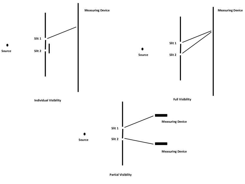
Figure 1. Possible ray visibilities for different experimental settings

Furthermore, the normalization condition (2.28) for a state vector in a Hilbert space also plays the role of the constraint (2.25) for the variational problem (2.24), and we interpret this constraint as the condition of certain occurrence of the external influence in laboratory space. Additionally, only solutions for a specific energy eigenvalue $E_{j}$ of the variational problem are observable in an individual measurement process by virtue of the consistency condition (2.14), and every detectable external influence must be an element of the energy eigenvalue basis. Therefore, energy eigenvalue superpositions are not detectable in laboratory space as confirmed by all quantum experiments.

Thus, in the case of the double-slit experiment with one slit closed for each measurement process, the Hilbert space of possible external influences $\mathcal{H}_{1}\oplus\mathcal{H}_{2}$ is the sum of the individual Hilbert space of external influences emanating from one individual slit, and the normalization conditions

(3.4) $$\int\left|\psi_{i}\right|^{2}dq=1,\ \ \ \ \ i=1,2$$

correspond to the certain event of appearance in laboratory space of the external influence originating from slit $i$ with given energy $E_{j}$, where we suppress the energy index $j$ in the following equations. Thus, the integral (3.4) over entire laboratory space expresses the certain appearance of an external influence in laboratory space originating from the individual slits. The integral over the interval $[x,x+\delta x]$ gives then the probability

(3.5) $$p_{i}(x)=\int_{x}^{x+\delta x}\left|\psi_{i}(q)\right|^{2}dq$$

to measure the external influence emanating from slit $i$ in this region and the total probability is the sum of the individual probabilities normed to 1, which is equivalent to the particle picture of standard quantum mechanics.

Let us consider now the Hilbert space of possible external influences originating from both slits. As mentioned above, this Hilbert space is degenerate and can be represented in two different energy eigenvalue bases. One possibility is to represent the states in the basis of individual functions $\psi_{1}$ and $\psi_{2}$ with energy eigenvalue $E_{j}$, which corresponds to the scenario of partial visibility as shown in the figure above. Then, each basis element $\psi_{i}$ is again subject to the consistency condition for the observability of a small external influence in laboratory space with normalization condition (2.28)

(3.6) $$\int\left|\psi_{i}\right|^{2}dq=1,\ \ \ \ \ i=1,2.$$

This leads again to the probability (3.5) of finding the particle in the interval $[x,x+\delta x]$ with energy $E_{j}$. But, analogous to the non-degenerate case a superposition state $\psi=\alpha_{1}\psi_{1}+\alpha_{2}\psi_{2}$ is not observable in laboratory space in this basis. Therefore, this basis describes exclusively the particle picture of the theory.

On the other hand, we can use the superposition state

(3.7) $$\psi=\left(\alpha_{1}\psi_{1}+\alpha_{2}\psi_{2}\right)$$

as the basis of the energy eigenvalue representation of the Hilbert space, which corresponds to full visibility of both slits at the instance in time and space of the quantum event. This basis allows us to identify the superposition state of the external influences with the normalization condition (2.28) which leads to the probability

(3.8) $$p_{i}(x)=\int_{x}^{x+\delta x}\left|\alpha_{1}\psi_{1}+\alpha_{2}\psi_{2}\right|^{2}dq$$

of finding the particle in the interval $[x,x+\delta x]$ with energy $E_{j}$. Since the $\psi_{i}$ are eigenstates of the degenerate eigenvalue $E_{j}$ these are not orthogonal and result into interference terms leading to the wave interpretation of the experiment. Now, the individual wave functions $\psi_{i}$ are superposition states and are not observable in this basis by virtue of the consistency condition. Thus, the complementary of wave and particle behaviour is a result of the basis change in a degenerate Hilbert space and no additional assumptions need to be introduced to explain this experimental fact.

4. Conclusion

Our view of quantum mechanics does not only allow the derivation of the Schrö-dinger equation and the Hilbert space of states from physically intuitive assumptions, but gives also an explanation of wave-particle duality. In contrast to standard quantum mechanics we do not need to incorporate additional concepts to explain the complementarity of waves and particles, but interpret this fact as the result of a basis change in a Hilbert space, which is closely tied to a quantum event of an experimental setting in a laboratory.

In addition, all considerations above apply to delayed choice experiments, as experimentally realized in e.g. [10], since our approach singles out for the quantum event of significance the laboratory space configuration at the definite point in time of appearance in the detector, which removes the paradox that a quantum objects changes its wave or particle nature during its experimental lifetime. The interpretation problems in traditional approaches stem from the implicit assumption of historic consistence which is connected to the tacit picture that the wave or particle property is attached to an object ”flying” from the source to the detector, which must therefore change its property during the ”flight”. In our case the time traceability of the quantum object, the small external influence, is reflected by the restriction to the family of consistent boundary conditions, which gives us the possibility to identify the quantum object at an arbitrary point in time by measuring in classical laboratory space. Thus, we can picture the same proposition that if we measured an electron at time $t_{1}$ we can conclude it is the same electron we would have measured at point $t_{2}$ somewhere else in the experimental set up. The difference, however, is that the small influence, which causes the quantum event, is explicitly external until its appearance in classical laboratory space and only the geometry of the classical configuration space at this point in time plays a crucial role. Therefore, we associate the wave or particle property of an object to a quantum event which is located at a specific point in time and space in laboratory space, which removes the paradoxical assumption that the particle must change its property over time.

However, this comes at the cost of a radical modification of quantum mechanics which is more on a conceptual level than a formal one. First, a quantum event is not an independent property of an object, but is always closely related to the experimental setting in laboratory space since the Hamilton-Jacobi equation for the external influence explicitly requires the Hamiltonian of the experimental environment. This is not a serious restriction as it enables us to show that the reduction of a state vector is equivalent to the transition of a possible external influence to an actual external influence which must be a basis element of the energy representation of the corresponding Hilbert space. In fact it enables us to show superposition states can only be measured for states of a degenerate energy eigenvalue and cannot be measured in an energy superposition state for different energies.

Second, the separation of the external influence from the laboratory system and the view of the wave function as a field in coordinate space only incorporate non-reality and non-locality into our derivation. Moreover, the explicit local construction of our approach and the separation between object space and laboratory space also removes the implicit assumption of absolute space given in the standard approach and introduces the concepts of non-reality and non-locality in a relative context between local spaces. We believe that our explicit incorporation of non-locality and non-reality into a local theory can be a first step to a better physical understanding of quantum mechanics as modern investigations and experiments give evidence that one has to give up the concepts of reality and locality in quantum mechanics [8],[9], [11], [12].

The author wants to thank M. Harris for reading the manuscript.

References

- [1] M. Aspelmeyer, Nature 464, 685-686 (2010).
- [2] I. M. Gelfand, S. V. Fomin, Calculus of Variations (Dover Publications,New York, 2000).
- [3] W. M. de Muynck, Foundations of quantum mechanics, an empiricist approach (Kluwer Academic Publishers, Dordrecht, 2002).
- [4] A. Peres, Quantum Theory: Concepts and Methods (Kluwer Academic Publishers, Dordrecht, 1993).
- [5] E. Schrödinger, Ann. Phys. 79, 361 (1926).
- [6] D. E. Kirk, Optimal Control Theory: An Introduction (Prentice-Hall, Englewood Cliffs, New Jersey, 1970).
- [7] R. Courant, D. Hilbert, Methoden der Mathematischen Physik I (Springer, Berlin, 4. Aufl., 1993).
- [8] Gröblacher et.al. Nature 446, 871 (2007).
- [9] A. J. Leggett, Found. of Phys. 33, 1469 (2003).
- [10] V. Jacques et al., Science 315, 966 (2007).
- [11] J.Bell, Physics 1, 195 (1964); reprinted in Bell, J. Speakable and Unspeakable in Quantum Mechanics, 14 (Cambridge Univ. Press, 2004).
- [12] A. Aspect,J. Dalibard, & G. Roger, Phys. Rev. Lett. 49, 1804 (1982).