RU-NHETC-2010-10

Quantum Sine(h)-Gordon Model

and
Classical Integrable Equations

S. L. Lukyanov and A. B. Zamolodchikov

NHETC, Department of Physics and Astronomy

Rutgers University

Piscataway, NJ 08855-0849, USA

and

L.D. Landau Institute for Theoretical Physics

Chernogolovka, 142432, Russia

Abstract

We study a family of classical solutions of modified sinh-Gordon equation, $\partial_{z}\partial_{{\bar{z}}}\eta-\mathrm{e}^{2\eta}+p(z)\,p({\bar{z}})\ \mathrm{e}^{-2\eta}=0$ with $p(z)=z^{2\alpha}-s^{2\alpha}$. We show that certain connection coefficients for solutions of the associated linear problem coincide with the $Q$-function of the quantum sine-Gordon $(\alpha>0)$ or sinh-Gordon $(\alpha<-1)$ models.

 

March 2010

To the memory of Alyosha Zamolodchikov

1 Introduction

In over three decades of study of quantum integrable systems, a remarkable (and largely mysterious) relation to classical integrable equations was observed in a number of different contexts. The first such relation was discovered long ago by Barouch, Tracy, and McCoy[1], who have derived the spin-spin correlation function in the Ising Field Theory in terms of special Painlevé III transcendent, i.e. the solution of the differential equation,

$$\frac{{\rm d}^{2}f}{{\rm d}\tau^{2}}+\frac{1}{\tau}\frac{{\rm d}f}{{\rm d}\tau}-\frac{1}{2}\ \sinh(2f)=0$$ (1.1)

which decays at $\tau\to\infty$ and is singular as $-\log(-\tau\log\tau)$ at $\tau\to 0$. The derivation relies on the free-field nature of the Ising Field Theory, and it is still unknown if this powerful result can be generalized in any simple way to interacting integrable quantum field theories.

However, relation to classical integrable equation has surfaced later in analysis of the dilute self-avoiding polymer problem [2, 3], which is related to quantum sine-Gordon model at special value of the coupling parameter. It was found that the off-critical partition function of a self-avoiding polymer loop on an infinite cylinder is expressed exactly through another solution of the same Painlevé III equation (1.1), this time with the singularity $-\frac{1}{3}\log t+O(1)$ at small $t$. This elegant result can be attributed to supersymmetry of the problem – it can be reformulated in terms of quantum sine-Gordon model at special value of its coupling constant ($\beta^{2}=\frac{2}{3}$ in (1.2) below), where it exhibits ${\cal N}=2$ supersymmetry. Indeed, the derivation in [4] has its roots in deep analysis of 2D ${\cal N}=2$ supersymmetric field theories [5]. At the same time, the finite-size partition function is generally much simpler object as compared to the correlation functions. In particular, TBA technique [7] can be employed to determine this quantity in any integrable quantum field theory (supersymmetric or not) as long as its S-matrix is known [8]. Therefore one may expect that some more or less direct extension of the results of [2, 3] to generic integrable theories is possible.

In this paper we propose such extension to the case of the quantum sine-Gordon model

$$\mathcal{L}=\frac{1}{16\pi}\ \left[\,\left(\partial_{t}\varphi\right)^{2}-\left(\partial_{x}\varphi\right)^{2}\,\right]+2\mu\,\cos\left(\beta\varphi\right)$$ (1.2)

at generic values of the coupling parameter $\beta^{2}<1$. Here $\mu$ sets the mass scale, $\mu\sim\text{[\,mass\,]}^{2-2\beta^{2}}$. We will consider the theory in finite-size geometry, with the spatial coordinate $x$ in $\varphi=\varphi(x,t)$ compactified on a circle of a circumference $R$, with the periodic boundary conditions

$$\varphi(x+R,t)=\varphi(x,t)\,.$$ (1.3)

Due to the periodicity of the potential term $2\mu\,\cos(\beta\varphi)$ in (1.2) in $\varphi$, the space of states $\mathcal{H}$ splits into orthogonal subspaces $\mathcal{H}_{k}$, characterized by the “quasi-momentum” $k$,

$$\varphi\to\varphi+2\pi/\beta\,:\qquad\mid\Psi_{k}\,\rangle\ \to\ \mathrm{e}^{2\pi\mathrm{i}\,k}\,\mid\Psi_{k}\,\rangle$$ (1.4)

for $\mid\Psi_{k}\,\rangle\in\mathcal{H}_{k}$. We call $k$-vacuum the ground-state of the finite-size system (1.2) in the sector $\mathcal{H}_{k}$.

The quantum field theory (1.2) is integrable, in particular it has infinite set of commuting local Integrals of Motion (IM) $\mathbb{I}_{2n-1},\ \mathbb{\bar{I}}_{2n-1}$, $2n=2,\,4,\,6,\,\ldots$ being the Lorentz spins of the associated local densities [6]. Of primary interest are the $k$-vacuum eigenvalues $I_{2n-1}(k\,|\,R),\ {\bar{I}}_{2n-1}(k\,|\,R)$, especially the $k$-vacuum energy $I_{1}+{\bar{I}}_{1}$. In principle, these quantities are accessible through the Thermodynamic Bethe Ansatz (TBA) technique, but the most efficient approach is the Destri-De Vega (DDV) equation [9, 10] (Similar equation was earlier derived in the lattice $XXZ$-model in Ref.[11]). The later determines the so-called $Q$-function $Q(\theta,k\,|\,R)$, whose asymptotic expansions at $\theta\to+\infty$ and $\theta\to-\infty$ generate the eigenvalues $I_{2n-1}$ and ${\bar{I}}_{2n-1}$ (along with the eigenvalues of the nonlocal integrals of motion of Ref.[12]), respectively. Remarkable observation of [2, 3] is that at the special value $\beta^{2}=\frac{2}{3}$ these essentially quantum characteristics can be related to the solution of the classical nonlinear differential equation (1.1).

Equation (1.1) of course is the radial equation for rotationally symmetric solutions of 2D sinh-Gordon equation. We will argue that for generic $\beta^{2}$ similar relation exists to the classical Modified Sinh-Gordon equation (MShG)

$$\partial_{z}\partial_{\bar{z}}\eta-\mathrm{e}^{2\eta}+p(z)\,{p}(\bar{z})\ \mathrm{e}^{-2\eta}=0$$ (1.5)

with the functions $p(z)$ of the form

$$p(z)=z^{2\alpha}-s^{2\alpha}\,.$$ (1.6)

Here $\alpha$ and $s$ are real, positive parameters, related to the parameters $\beta$, $\mu$ in (1.2) as follows

$$\alpha=\beta^{-2}-1\,,\qquad\qquad s=\Big{(}\frac{R}{\pi\beta^{2}}\Big{)}^{\beta^{2}}\ \bigg{[}\,\frac{\mu\pi\Gamma(1-\beta^{2})}{\Gamma(\beta^{2})}\,\bigg{]}^{\frac{\beta^{2}}{2-2\beta^{2}}}\ ,$$ (1.7)

but $z,\ \bar{z}$ are formal variables, not related to the space-time coordinates $(x,\,t)$ in (1.2). Equation (1.5) with general $p(z)$ is well known in differential geometry (see [13] for review). The same equation with polynomial $p(z)$ has emerged lately in different contexts in SUSY gauge theories [14, 15, 17, 16, 18], and these later papers have inspired to large extent the work presented here.

Obviously, MShG equation in general has no rotational symmetry. Instead, it has discrete symmetry

$$z\to\text{e}^{\frac{\mathrm{i}\pi}{\alpha}}\ z\,,\qquad\bar{z}\to\text{e}^{-\frac{\mathrm{i}\pi}{\alpha}}\ {\bar{z}}\ .$$ (1.8)

We will consider solutions of MShG equation (1.5) which respect this symmetry, continuous at all finite nonzero $z,\bar{z}$, and grow slower then exponential at $z,\bar{z}\to\infty$ (precise conditions are listed in Section 2). There is one-parameter set of such solutions, characterized by the behavior $\eta\to l\,\log(z\bar{z})$ at $z,\bar{z}\to 0$, with real $l\in[-\frac{1}{2},\,\frac{1}{2}\,]$ which will turn out to be related to the quasi-momentum as

$$l=2\,|k|-{\textstyle\frac{1}{2}}\ .$$ (1.9)

As is well known, the MShG equation is integrable, and the associated linear problem has the form [19]

$${\boldsymbol{D}}{\bf\Psi}=0\,,\qquad{\bar{\boldsymbol{D}}}{\bf\Psi}=0\ ,$$ (1.10)

where ${\boldsymbol{D}},\,{\bar{\boldsymbol{D}}}$ are components of $sl(2)$ connection

$${\boldsymbol{D}} = \partial_{z}+{\textstyle\frac{1}{2}}\ \partial_{z}\eta\ \sigma^{3}-\mathrm{e}^{\theta}\ \ \big{[}\,\sigma^{+}\ \mathrm{e}^{\eta}+\sigma^{-}\ p(z)\,\mathrm{e}^{-\eta}\,\big{]}\ ,$$ (1.11)

$${\bar{\boldsymbol{D}}} = {\partial}_{\bar{z}}-{\textstyle\frac{1}{2}}\ {\partial}_{\bar{z}}\eta\ \sigma^{3}-\mathrm{e}^{-\theta}\,\big{[}\,\sigma^{-}\ \mathrm{e}^{\eta}+\sigma^{+}\ p({\bar{z}})\,\mathrm{e}^{-\eta}\,\big{]}\ ,$$

with the spectral parameter $\theta$. The $Q$-function of the quantum sine-Gordon model (1.2) will be related to connection coefficients for certain solution of the linear problem (1.10). Therefore our result can be regarded as generalization to $\mu\not=0$ of the relation [20] between the integrable structures of CFT [21, 22, 23] and spectral characteristics of linear ordinary differential equations [24, 25]. Indeed, our derivation follows very closely the analysis in [26]. The novel feature of the massive case is that the coefficients in the linear problem are not elementary functions but rather solutions of integrable nonlinear partial differential equation (1.5).

Similar relation exists between certain solution of the MShG equation (1.5), with $p(z)$ of the same form (1.6) but this time with $\alpha<-1$,

$$\alpha=-b^{-2}-1\ ,\qquad s=\Big{(}\frac{R}{\pi b^{2}}\Big{)}^{-b^{2}}\ \bigg{[}-\frac{\mu\pi\Gamma(1+b^{2})}{\Gamma(-b^{2})}\,\bigg{]}^{\frac{b^{2}}{2+2b^{2}}}$$ (1.12)

and the vacuum $Q$-function of the quantum sinh-Gordon model

$$\mathcal{L}=\frac{1}{16\pi}\ \left[\,\left(\partial_{t}\varphi\right)^{2}-\left(\partial_{x}\varphi\right)^{2}\,\right]-2\mu\,\cosh\left(b\varphi\right)\ ,$$ (1.13)

where again the spatial finite size geometry (1.3) is assumed. Of course, physical content of the quantum sinh-Gordon model is much different from the sine-Gordon model (1.2). In particular, (1.13) has unique vacuum. Correspondingly, the MShG equation (1.5) with $\alpha<-1$ has unique solution which is continuous at all finite nonzero $z,\bar{z}$. The vacuum $Q$-function of (1.13) [27, 28, 29] will be related to the linear problem (1.10) associated with this unique solution.

The paper is organized as follows. In Section 2 we discuss the MShG equation with $\alpha>0$. We define a family of regular solutions, and describe their basic properties. We also discuss the associated linear problem (1.10), and define the functions $Q_{+}(\theta),\ Q_{-}(\theta)$ as certain connection coefficients. In Section 3 we describe how the function $Q(\theta,k)$ is constructed out of these coefficients, and list its basic properties. In particular, we show that it is determined by unique solution of complex nonlinear integral equation identical to DDV equation, and thus coincides with the vacuum $Q$-function of the sine-Gordon model. We also establish relation between the classical local IM of MShG, and vacuum eigenvalues of the quantum IM of the sine-Gordon model. In Section 4 we define the functions $T_{j}(\theta,k)$ in terms of the monodromy of the linear problem (1.10), and show that they coincide with the vacuum $T$-functions of the model (1.2). In particular, at integer values of $2\alpha$ these functions can be determined through the finite system of TBA equations, which were previously derived in similar context in [14, 15, 17, 16, 18]. The relation is similar to that described in Ref.[30] in the massless case. Section 5 is devoted to analysis of the inverse scattering problem in (1.10). In particular, we present explicit series-like representation of the solution $\eta$. MShG with $\alpha<-1$, and its relation to the quantum sinh-Gordon model (1.13), is discussed in Section 6.

2 MShG equation and linear problem

Although generally $z$ and $\bar{z}$ in (1.5) can be regarded as independent complex variables, in the present discussion we usually (but not always) assume them to be complex coordinates on 2D real space. Thus, $\eta$ in (1.5) is assumed to be a function of two real variables, $\eta=\eta(\rho,\phi)$, the polar coordinates associated with $(z,\bar{z})$,

$$z=\rho\,\mathrm{e}^{\mathrm{i}\phi}\,,\qquad\qquad\bar{z}=\rho\,\mathrm{e}^{-\mathrm{i}\phi}\,.$$ (2.1)

We consider special family of solutions of (1.5), parameterized by real $l\in\big{[}-\frac{1}{2},\frac{1}{2}\big{]}$, defined by the following properties:

i) Periodicity

$$\eta\big{(}\rho,\phi+{\textstyle\frac{\pi}{\alpha}}\big{)}=\eta(\rho,\phi)\,.$$ (2.2)

In other words, the solutions $\eta(\rho,\phi)$ are single-valued functions on a cone with the apex angle $\frac{\pi}{\alpha}$,

$${\mathbb{C}}_{\frac{\pi}{\alpha}}\,:\quad\phi\sim\phi+{\textstyle\frac{\pi}{\alpha}}\,,\qquad 0\leq\rho<\infty\,.$$ (2.3)

ii) $\eta(\rho,\phi)$ are real-valued and finite everywhere on the cone $\mathbb{C}_{\frac{\pi}{\alpha}}$, except for the apex $\rho=0$.

iii) Large-$\rho$ asymptotic form

$$\eta(\rho,\phi)=\alpha\,\log\rho+o(1)\qquad\text{as}\quad\rho\to\infty\,.$$ (2.4)

iv) $\rho\to 0$ asymptotic form

$$\eta(\rho,\phi)=\begin{cases}2l\,\log\rho+O(1)\qquad\qquad\quad\quad\quad\text{for}\quad|l|<{\textstyle\frac{1}{2}}\\ \pm\,\log\rho+O\big{(}\log(-\log\rho)\big{)}\qquad\ \text{for}\quad l=\pm{\textstyle\frac{1}{2}}\end{cases}\ \ \qquad\text{as}\quad\rho\to 0\ .$$ (2.5)

Unless specified otherwise, we will describe the cone (2.3) by the chart,

$${\cal M}_{z}^{(0)}\ :\ \ \ \ \ \ \ \ -{\textstyle{\pi\over 2\alpha}}\leq\phi\leq{\textstyle{\pi\over 2\alpha}}\,,\qquad 0\leq\rho<\infty$$ (2.6)

with the rays $\phi=-{\pi\over 2\alpha}$ and $\phi={\pi\over 2\alpha}$ identified. We assume that solution satisfying conditions i)-iv) is unique, and hence respects all symmetries of Eq.(1.5). In particular,

$$\eta(\rho,\,\phi)=\eta(\rho,-\phi)\ .$$ (2.7)

Starting from the asymptotic form (2.5) one can develop $z,\bar{z}\to 0$ expansion of the form

$$\eta = l\ \log(z\bar{z})+\eta_{0}+\sum_{k=1}^{\infty}\gamma_{k}\ \big{(}\,z^{2\alpha k}+{\bar{z}}^{2\alpha k}\,\big{)}$$

$$- {s^{4\alpha}\,\mathrm{e}^{-2\eta_{0}}\over(1-2l)^{2}}\ \ (z\bar{z})^{1-2l}+{\mathrm{e}^{2\eta_{0}}\over(1+2l)^{2}}\ \ (z{\bar{z}})^{1+2l}+\ldots\ ,$$

where $\eta_{0}$ and $\gamma_{k}$ are integration constants. It is easy to see that the coefficients in all omitted terms in this expansion are uniquely determined once these integration constants are given. On the other hand, $\eta_{0}$ and $\gamma_{k}$ are not new parameters of the solution; they have to be determined from consistency of this expansion with the remaining conditions i)-iii). We will give explicit form of the constant $\eta_{0}$ in Section 3 below (see Eqs.(3.14), (3.40)).

The expansion (2) remains valid if we regard $z$ and $\bar{z}$ as independent complex variables. For our analysis, the most important message from (2) is that in the “light-cone” limit $\bar{z}\to 0$ (with fixed $z$)

$$\eta\to l\,\log(z\bar{z})+\eta_{0}+\gamma(z)\,,$$ (2.9)

where $\gamma(z)=\sum_{k=1}^{\infty}\gamma_{k}\,z^{2\alpha k}$ decays as

$$\gamma(z)\sim z^{2\alpha}$$ (2.10)

at small $z$.

Although the solution $\eta(\rho,\phi)$ is a single-valued functions on the cone (2.3), the connection (1.11) is not. Instead, the linear problem (1.10) is invariant with respect to the operation

$${\hat{\Omega}}\,:\qquad\phi\to\phi+{\textstyle\frac{\pi}{\alpha}}\,,\quad\theta\to\theta-{\textstyle\frac{\mathrm{i}\pi}{\alpha}}\,,$$ (2.11)

involving the shift of the spectral parameter $\theta$. Another easily established symmetry of this linear problem involves the operation

$${\hat{\Pi}}\,:\qquad\theta\to\theta-\mathrm{i}\pi\,,$$ (2.12)

which transforms the connection (1.11) as

$${\hat{\Pi}}[\,{\boldsymbol{D}}\,]=\sigma^{3}\,{\boldsymbol{D}}\,\sigma^{3}\,,\qquad{\hat{\Pi}}[\,{\bar{\boldsymbol{D}}}\,]=\sigma^{3}\,{\bar{\boldsymbol{D}}}\,\sigma^{3}\,.$$ (2.13)

Motivated by these mutually commuting symmetries, we define two solutions ${\bf\Psi}_{\pm}={\bf\Psi}_{\pm}(\rho,\phi\,|\,\theta)$ of the linear problem (1.10) uniquely specified by their asymptotic behavior

$${\boldsymbol{\Psi}}_{+}\to{1\over\sqrt{\cos(\pi l)}}\ \begin{pmatrix}0\\ \mathrm{e}^{(\mathrm{i}\phi+\theta)l}\end{pmatrix}\ ,\ \ \ \ \ {\boldsymbol{\Psi}}_{-}\to{1\over\sqrt{\cos(\pi l)}}\ \begin{pmatrix}\mathrm{e}^{-(\theta+\mathrm{i}\phi)l}\\ 0\end{pmatrix}\ \ \ \ \ {\rm as}\ \ \ \ \rho\to 0\,.$$ (2.14)

In writing (2.14) we have assumed that $|l|<\frac{1}{2}$. In the analysis below we usually adopt this limitation, and treat the case $|l|=\frac{1}{2}$ by continuity. Using Eqs.(2.11)-(2.14), and the fact that at real $\theta$

$${\bar{\boldsymbol{D}}}(\theta)=\sigma^{1}\,{\boldsymbol{D}}^{*}(-\theta)\,\sigma^{1}\ ,$$ (2.15)

where the star denotes complex conjugation and $\sigma^{1}=\sigma^{+}+\sigma^{-}$, it is straightforward to establish the following properties of these solutions:

• ${\boldsymbol{\Psi}}_{\pm}(\rho,\phi\,|\,\theta)$ are entire functions of $\theta$ for arbitrary real $\phi$ and $\rho>0$.

• ${\hat{\Omega}}$-invariance:

  $${\boldsymbol{\Psi}}_{\pm}\big{(}\rho,\phi+{\textstyle{\pi\over 2\alpha}}\,|\,\theta-{\textstyle{\mathrm{i}\pi\over 2\alpha}}\big{)}=\ {\boldsymbol{\Psi}}_{\pm}(\rho,\phi-{\textstyle{\pi\over 2\alpha}}\,|\,\theta+{\textstyle{\mathrm{i}\pi\over 2\alpha}})\ .$$ (2.16)

• ${\hat{\Pi}}$-transformation

  $${\boldsymbol{\Psi}}_{+}(\rho,\phi\,|\,\theta\pm\mathrm{i}\pi) = -\mathrm{e}^{\pm\mathrm{i}\pi l}\ \sigma^{3}\ {\boldsymbol{\Psi}}_{+}(\rho,\phi\,|\,\theta)\,,$$ (2.17)

  $${\boldsymbol{\Psi}}_{-}(\rho,\phi\,|\,\theta\pm\mathrm{i}\pi) = \ \ \mathrm{e}^{\mp\mathrm{i}\pi l}\ \sigma^{3}\ {\boldsymbol{\Psi}}_{-}(\rho,\phi\,|\,\theta)\ .$$

• Normalization condition

  $$\det({\boldsymbol{\Psi}}_{+},\,{\boldsymbol{\Psi}}_{-})=-{1\over\cos(\pi l)}\ .$$ (2.18)

  Here and below $({\boldsymbol{\Psi}}_{+},\,{\boldsymbol{\Psi}}_{-})$ stands for the $2\times 2$ matrix with the columns ${\boldsymbol{\Psi}}_{+}$ and ${\boldsymbol{\Psi}}_{-}$.

• For real $\theta$

  $${\boldsymbol{\Psi}}^{*}_{\pm}(\rho,\phi\,|\,\theta)=\sigma^{1}\,{\boldsymbol{\Psi}}_{\mp}(\rho,\phi\,|\,-\theta)\ ,$$ (2.19)

  and

  $${\boldsymbol{\Psi}}_{\pm}^{*}(\rho,\,0\,|\,\theta)={\boldsymbol{\Psi}}_{\pm}(\rho,\,0\,|\,\theta)\ .$$ (2.20)

Note also that for $l\to\pm\frac{1}{2}$:

$$\lim_{l\to\pm\frac{1}{2}}\,\big{[}\,\cos(\pi l)\,({\boldsymbol{\Psi}}_{+}-{\boldsymbol{\Psi}}_{-})\,\big{]}=0\ .$$ (2.21)

The above solutions ${\boldsymbol{\Psi}}_{\pm}$ are specified by their $\rho\to 0$ behavior (2.14). On the other hand, at large $\rho$ the WKB analysis applies. Assuming that $\theta$ is real, it is straightforward to show that while generic solution of (1.10) grows exponentially at $\rho\to\infty$, there is a solution which decays in the wedge

$$-{\textstyle{\pi\over 2(\alpha+1)}}\leq\phi\leq{\textstyle{\pi\over 2(\alpha+1)}}\ .$$ (2.22)

We denote this decaying solution as ${\boldsymbol{\Xi}}={\boldsymbol{\Xi}}(\rho,\phi\,|\,\theta)$. It is uniquely specified by the asymptotic condition

$${\boldsymbol{\Xi}}(\rho,\phi\,|\,\theta)\to{\boldsymbol{\cal E}}_{-}(\rho,\phi\,|\,\theta)\ \ \ \ \ \ {\rm as}\ \ \ \ \rho\to+\infty\ ,$$ (2.23)

where ${\boldsymbol{\cal E}}_{-}$ is the shorthand for the decaying exponential

$${\boldsymbol{\cal E}}_{-}=\begin{pmatrix}\mathrm{e}^{-{\mathrm{i}\alpha\phi\over 2}}\\ -\mathrm{e}^{{\mathrm{i}\alpha\phi\over 2}}\end{pmatrix}\ \exp\bigg{[}\,-{2\rho^{\alpha+1}\over\alpha+1}\ \cosh(\theta+\mathrm{i}(\alpha+1)\phi\big{)}\,\bigg{]}\ .$$ (2.24)

Since ${\boldsymbol{\Psi}}_{\pm}$ form a basis in the space of solutions of linear problem (1.10), we have linear relation

$${\boldsymbol{\Xi}}=Q_{-}(\theta)\ {\boldsymbol{\Psi}}_{+}+Q_{+}(\theta)\ {\boldsymbol{\Psi}}_{-}\ ,$$ (2.25)

where the coefficients $Q_{\pm}(\theta)$ (of course independent of the variables $\rho,\phi$) are functions of the spectral parameter $\theta$ as well as the parameter $l$ (the last argument is temporarily omitted in the above notations). These coefficients are to be related to the $Q$-function of the quantum sine-Gordon model (1.2).

As is well known, the matrix linear problem (1.10) can be reduced to second order linear differential equations. One can write general solution of (1.10) as

$${\boldsymbol{\Psi}}=\begin{pmatrix}\mathrm{e}^{{\theta\over 2}}\ \mathrm{e}^{\eta\over 2}\ \psi\\ \mathrm{e}^{-{\eta\over 2}}\ \mathrm{e}^{-{\theta\over 2}}\,(\partial_{z}+\partial_{z}\eta)\,\psi\end{pmatrix}=\begin{pmatrix}\mathrm{e}^{-{\eta\over 2}}\ \mathrm{e}^{\theta\over 2}\,(\partial_{\bar{z}}+\partial_{\bar{z}}\eta)\,{\bar{\psi}}\\ \mathrm{e}^{{\eta\over 2}}\ \mathrm{e}^{-{\theta\over 2}}\ {\bar{\psi}}\end{pmatrix}\ ,$$ (2.26)

where $\psi$ and ${\bar{\psi}}$ solve the equations

$$\big{[}\,\partial_{z}^{2}-u(z,{\bar{z}})-\mathrm{e}^{2\theta}\ \ p(z)\,\big{]}\ \psi=0\ ,$$ (2.27)

$$\big{[}\,\partial^{2}_{\bar{z}}-{\bar{u}}(z,{\bar{z}})-\mathrm{e}^{-2\theta}\,{p}({\bar{z}})\,\big{]}\ {\bar{\psi}}=0\ ,$$ (2.28)

with

$$u(z,{\bar{z}})=(\partial_{z}\eta)^{2}-\partial_{z}^{2}\eta\ ,\ \ \ \ {\bar{u}}(z,{\bar{z}})=({\partial}_{\bar{z}}\eta)^{2}-{\partial}^{2}_{\bar{z}}\eta\ .$$ (2.29)

This form is convenient for making connection to the analysis in Ref.[26] which emerges at small $s$ and large $\theta$. Concentrating attention on (2.27), consider first the light cone limit $\bar{z}\to 0$ in which $\eta$ assumes the form (2.9). After that, the limit $z\sim s\to 0\,,\ \theta\to+\infty$ can be taken, with the combinations

$$x=\mathrm{e}^{{\theta\over 1+\alpha}}\ z\ ,\ \ \ \ \ \qquad E=s^{2\alpha}\ \mathrm{e}^{{2\theta\alpha\over 1+\alpha}}\ ,$$ (2.30)

kept finite. Then the term $\gamma(z)$ in (2.9) can be dropped, and (2.27) reduces to the Schr${\rm\ddot{o}}$dinger equation

$$\bigg{[}\,-\partial_{x}^{2}+{l(l+1)\over x^{2}}+x^{2\alpha}\,\bigg{]}\ \psi=E\ \psi\ .$$ (2.31)

In this double limit the solutions ${\bf\Psi}_{\pm}$ assume asymptotic form

$${\boldsymbol{\Psi}}_{+} \to {\mathrm{e}^{{\alpha\theta(2l+1)\over 2(\alpha+1)}}\over(2l+1)\sqrt{\cos(\pi l)}}\ \ \ \ \begin{pmatrix}(z\bar{z})^{l\over 2}\ \ \mathrm{e}^{{\theta\alpha\over 2(\alpha+1)}}\ \psi_{+}(x)\\ \\ (z\bar{z})^{-{l\over 2}}\,\mathrm{e}^{-{\alpha\theta\over 2(\alpha+1)}}\ (\partial_{x}+{l\over x})\,\psi_{+}(x)\end{pmatrix}\ ,$$

$${\boldsymbol{\Psi}}_{-} \to {\mathrm{e}^{-{\alpha\theta(2l+1)\over 2(\alpha+1)}}\over\sqrt{\cos(\pi l)}}\ \ \ \ \begin{pmatrix}(z\bar{z})^{l\over 2}\ \ \mathrm{e}^{{\theta\alpha\over 2(\alpha+1)}}\ \psi_{-}(x)\\ \\ (z\bar{z})^{-{l\over 2}}\,\mathrm{e}^{-{\alpha\theta\over 2(\alpha+1)}}\ (\partial_{x}+{l\over x})\,\psi_{-}(x)\end{pmatrix}\ ,$$ (2.32)

where $\psi_{\pm}$ are unique solutions of the above Schr${\rm\ddot{o}}$dinger equation (2.31) defined for $|l|<{1\over 2}$ by their $x\to 0$ behavior

$$\psi_{+}\to x^{l+1}\,,\qquad\psi_{-}\to x^{-l}\ .$$

The equation (2.25) then reduces to

$$\chi=Q_{-}^{(\text{cft})}(\theta-\theta_{s})\ \psi_{+}+Q_{+}^{(\text{cft})}(\theta-\theta_{s})\ \psi_{-}\ ,$$ (2.33)

where $\chi$ is the decaying solution of (2.31), defined by the asymptotic condition

$$\chi\to x^{-\frac{\alpha}{2}}\ \exp\Big{[}-\frac{x^{\alpha+1}}{\alpha+1}+O\big{(}x^{1-\alpha}\big{)}\,\Big{]}\ \ \ \ \ {\rm as}\ \ x\to+\infty\ ,$$ (2.34)

and $\theta_{s}=-(\alpha+1)\ \log(s)$. The coefficients $Q_{\pm}^{\rm(cft)}(\theta)$ coincide with the $Q$-functions (the vacuum eigenvalues of the operators ${\bf Q}_{\pm}(\theta)$ defined in [22, 23]) of the left-moving chiral sector of the CFT emerging in the massless case $\mu=0$ in (1.2). The proof of this statement is given in Ref.[26]. Eq.(2.25) generalizes (2.33) to the massive case $\mu\neq 0$.

3 $Q$-function

3.1 Basic properties

The following properties are established by arguments nearly identical to those presented in Ref.[26] (For completeness we sketch the derivations in Appendix A)

• $Q_{\pm}(\theta)$ are entire, quasiperiodic functions of $\theta$,

  $$Q_{\pm}\big{(}\theta+{\textstyle{\mathrm{i}\pi\over 2}}+{\textstyle{\mathrm{i}\pi\over 2\alpha}}\big{)}=\mathrm{e}^{\pm\mathrm{i}\pi(l+{1\over 2})}\ \ Q_{\pm}\big{(}\theta-{\textstyle{\mathrm{i}\pi\over 2}}-{\textstyle{\mathrm{i}\pi\over 2\alpha}}\big{)}\ .$$ (3.1)

• At real $\theta$

  $$Q^{*}_{\pm}(\theta)=Q_{\pm}(\theta)\ ,\ \ \ \ \ Q_{\pm}(\theta)=Q_{\mp}(-\theta)\ .$$ (3.2)

• $Q_{\pm}(\theta)$ satisfy the Quantum Wronskian relation

  $$Q_{+}(\theta+{\textstyle{\mathrm{i}\pi\over 2\alpha}})Q_{-}(\theta-{\textstyle{\mathrm{i}\pi\over 2\alpha}})-Q_{+}(\theta-{\textstyle{\mathrm{i}\pi\over 2\alpha}})Q_{-}(\theta+{\textstyle{\mathrm{i}\pi\over 2\alpha}})=-2\mathrm{i}\ \cos(\pi l)\ .$$ (3.3)

• $$\lim_{l\to\pm\frac{1}{2}}Q_{+}(\theta)=\lim_{l\to\pm\frac{1}{2}}Q_{-}(\theta)\ .$$ (3.4)

We now define the function $Q(\theta,k)$ of complex $\theta$ and real $k$ as follows. For $k\in(-{1\over 2},\,{1\over 2})\backslash 0$ we set

$$Q(\theta,k):=\begin{cases}Q_{+}(\theta)\big{|}_{l=2k-{1\over 2}}\ \ \ &{\rm for}\ \ 0<k<{\textstyle{1\over 2}}\\ Q_{-}(\theta)\big{|}_{l=-2k-{1\over 2}}\ \ \ &{\rm for}\ \ -{\textstyle{1\over 2}}<k<0\end{cases}\ .$$ (3.5)

Due to the property (3.4) this definition extends to $k=0,\ k=\pm\frac{1}{2}$ by continuity, and then admits continuous periodic extension to all real $k$ by

$$Q(\theta,k)=Q(\theta,k+1)\ .$$ (3.6)

Thus defined, $Q(\theta,k)$ is entire function of $\theta$, satisfying

$$Q\big{(}\theta+{\textstyle{\mathrm{i}\pi(\alpha+1)\over\alpha}},\,k\big{)}=\mathrm{e}^{2\pi\mathrm{i}k}\ Q\big{(}\theta,\,k)\ ,$$ (3.7)

$$Q^{*}(\theta,k)=Q(\theta^{*},k)\ ,\ \ \ Q(-\theta,k)=Q(\theta,-k)\ ,$$ (3.8)

and

$$Q(\theta+{\textstyle{\mathrm{i}\pi\over 2\alpha}},k)\,Q(\theta-{\textstyle{\mathrm{i}\pi\over 2\alpha}},-k)-Q(\theta-{\textstyle{\mathrm{i}\pi\over 2\alpha}},k)\,Q(\theta+{\textstyle{\mathrm{i}\pi\over 2\alpha}},-k)=-2\mathrm{i}\,\sin(2\pi k)\ .$$ (3.9)

To fix the function $Q(\theta,k)$ uniquely, we will need two additional analytic properties. One concerns with the asymptotic behavior at $|\Re e\,(\theta)|\to\infty$, another determines the general pattern of zeros of this function in the complex $\theta$-plane. Due to the quasi-periodicity (3.7) one can concentrate attention on the strip

$$H\ :\ \ \big{|}\Im m\,(\theta)\big{|}\leq{\textstyle{\pi(\alpha+1)\over 2\alpha}}\ .$$ (3.10)

Define also

$$H_{+}\ :\ \ \ 0<\Im m(\theta)<{\textstyle{\pi(1+\alpha)\over\alpha}}\ ;\ \ \ \ \ \ H_{-}\ :\ \ \ -{\textstyle{\pi(1+\alpha)\over\alpha}}<\Im m\,\theta<0\ .$$ (3.11)

Then

• For real $k$ and $\alpha^{-1}\not=1,\,3,\,5\ldots$ ,

  $$Q \to \mathrm{e}^{\pm\mathrm{i}\pi k}\,{\mathfrak{S}}^{1\over 2}\ \exp\bigg{[}\,{r\,\mathrm{e}^{\theta\mp{\mathrm{i}\pi(1+\alpha)\over 2\alpha}}\over 4\cos({\pi\over 2\alpha})}\,\bigg{]}\ \ \ \ \ \ \Big{(}\,\theta\in H_{\pm}\,,\ \Re e\,(\theta)\to+\infty\,\Big{)}$$ (3.12)

  $$Q \to \mathrm{e}^{\pm\mathrm{i}\pi k}\,{\mathfrak{S}}^{-{1\over 2}}\ \exp\bigg{[}\,{r\,\mathrm{e}^{-\theta\pm{\mathrm{i}\pi(1+\alpha)\over 2\alpha}}\over 4\cos({\pi\over 2\alpha})}\,\bigg{]}\ \ \Big{(}\,\theta\in H_{\pm}\,,\ \Re e\,(\theta)\to-\infty\,\Big{)}\ .$$

  Here

  $$r=B\ s^{1+\alpha}\ ,\ \ \ \ \ \ \ \ \ \ B={2\sqrt{\pi}\Gamma(1+{1\over 2\alpha})\over\Gamma({3\over 2}+{1\over 2\alpha})}\ ,$$ (3.13)

  and ${\mathfrak{S}}$ is related to the constant $\eta_{0}$ in Eq. (2) as follows:

  $${\mathfrak{S}}={\Gamma(2k)\over\Gamma(1-2k)}\ 2^{4k-1}\ \mathrm{e}^{\eta_{0}}\ \ \ \ \ \ \ \ \ \ \ \ (0\leq k<{\textstyle\frac{1}{2}})\ .$$ (3.14)

  ${\mathfrak{S}}={\mathfrak{S}}(k)$ is a real function of real variable $k$, such that

  $${\mathfrak{S}}(k)\,{\mathfrak{S}}(-k)=1\ ,\ \ \ \ \ {\mathfrak{S}}(k+1)={\mathfrak{S}}(k)\ .$$ (3.15)

• For any real $k$, all the zeros of $Q(\theta,k)$ in the strip $H$ are real, simple, and accumulate towards $\theta\to\pm\infty$. Let

  $$\epsilon(\theta)=\mathrm{i}\ \log\left[\,\frac{Q\left(\theta+\frac{\mathrm{i}\pi}{\alpha},\,k\right)}{Q\left(\theta-\frac{\mathrm{i}\pi}{\alpha},\,k\right)}\,\right]\ ,$$ (3.16)

  where the branch of the log is fixed by the condition

  $$\epsilon(\theta)-\frac{r\,\mathrm{e}^{\theta}}{2\cos(\frac{\pi}{2\alpha})}\ \to\ -2\pi\,k\qquad\text{for}\quad\Re e(\theta)\to+\infty\quad\text{and}\quad|\Im m(\theta)|<{\textstyle\frac{\pi}{2}}\ .$$ (3.17)

  Then the zeros $\theta_{n}$ can be labeled by consecutive integers $n=0,\,\pm 1,\,\pm 2,\,\ldots\,$, so that $\theta_{n}<\theta_{n+1}$, and

  $$\epsilon(\theta_{n})=\pi\ (2n+1)\ .$$ (3.18)

The asymptotics (3.12) can be established through straightforward WKB analyses of the linear differential equations (1.10). The second property is derived in the next subsection.

3.2 Zeroes

Consider first the limit of small $s$. Due to the relations (3.6) and (3.8) we can assume, without loose of generality, that $0\leq k\leq\frac{1}{2}$. In this case the problem reduces to Schr${\rm\ddot{o}}$dinger equation (2.31), and the limiting pattern of zeros of $Q(\theta,k)$ can be read out from the pattern of zeros of $Q_{\pm}^{\rm(cft)}(\theta)$, which is relatively well understood [22, 26]. Simple analysis shows that in this case the zeros $\{\theta_{n}\}$ split into two widely separated groups, the “positive” zeros $\{\theta_{n}\}|_{n=0}^{\infty}$, and the “negative” zeros $\{\theta_{-n-1}\}|_{n=0}^{\infty}$. The limiting behavior of the positive zeros follows from Eqs.(2.30)-(2),

$$s^{2\alpha}\ \mathrm{e}^{2\alpha\theta_{n}\over\alpha+1}\ \to\ {\cal E}_{n}(l)\ ,$$ (3.19)

where $\big{\{}{\cal E}_{n}(l)\big{\}}\big{|}_{n=0}^{\infty}$ are eigenvalues of Schr${\rm\ddot{o}}$dinger operator (2.31) associated with the spectral problem

$$\psi \to x^{l+1}\ \ \ {\rm as}\ \ \ x\to 0$$ (3.20)

$$\psi \to 0\ \ \ \ \ \ \ {\rm as}\ \ \ x\to+\infty\ ,$$

with $l=2k-\frac{1}{2}$. If $l>-\frac{1}{2}$ the spectral problem (2.31), (3.20) corresponds to self-conjugated Schr${\rm\ddot{o}}$dinger operator, and the associated eigenvalues are non-degenerate and positive. In fact, it is possible to show that $\big{\{}{\cal E}_{n}(l)\big{\}}_{n=0}^{\infty}$ is a family of meromorphic functions of complex $l$. Furthermore, they are analytic in the strip $\Re e\,(l)\geq-\frac{3}{2}$ and ${\cal E}_{n}(l)>0$ for real $l>-\frac{3}{2}$. At $l=-\frac{3}{2}$ we have ${\cal E}_{0}(-\frac{3}{2})=0$, while all higher ${\cal E}_{n}(l)$ $(n=1,\,2\ldots)$ remain positive. Therefore at $s\to 0$ all the positive zeros are real, simple and have the limiting behavior (3.20) for any $k\in\big{[}0,\,\frac{1}{2}\big{]}$, including the ends of the segment.

The limiting behavior of the negative zeros is slightly more delicate, but still can be described by equation similar to (3.19),

$$s^{2\alpha}\ \mathrm{e}^{-{2\alpha\theta_{-n-1}\over\alpha+1}}\ \to{\cal E}_{n}(-1-l)\ .$$ (3.21)

Here the argument $-1-l$ belongs to the segment $\big{[}-\frac{3}{2},-\frac{1}{2}\big{]}$, where ${\cal E}_{n}(-1-l)$ are understood as the analytic continuations from the domain $\Re e(l)>\frac{1}{2}$. It is important that all ${\cal E}_{n}(-1-l)$ remain strictly positive, except for ${\cal E}_{0}(-1-l)$, which turns to zero at $l=\frac{1}{2}$. Thus the limiting behavior of the negative zeros is similar to the positive ones, i.e. they are also real and simple. If $s$ is small but finite, at $k\to\frac{1}{2}$ the single zero $\theta_{-1}$ leaves the group of negative zeroes and travels toward the positive ones. In the process, $\theta_{-1}$ remains real for any $0\leq k<\frac{1}{2}$, since $Q(\theta,\,k)$ is a real analytic function. For $k=\frac{1}{2}$ and arbitrary $s>0$ we have $\theta_{-1}\sim 1$, and hence it still formally obeys Eq.(3.21).

By continuity in $s$ (which we assume) this pattern of well separated groups of positive and negative zeros persists for sufficiently small values of this parameter. While exact locations of the zeros change with $s$, no additional zeros can be generated, since this would violate the asymptotics form (3.12), which is valid for any $s$. One can define two positive and non-degenerate sets of numbers $\big{\{}E_{n}(\pm k)\big{\}}|_{n=0}^{\infty}$ by

$$\mathrm{e}^{2\alpha\theta_{n}\over\alpha+1}=\begin{cases}\ s^{-2\alpha}\ E_{n}(k)\ ,\ \ \ \ \ \ \ \ \ \ &n\geq 0\\ \ s^{2\alpha}\ E^{-1}_{-n-1}(-k)\ ,\ \ \ &n<0\end{cases}\ .$$ (3.22)

In the domain $0\leq k\leq\frac{1}{2}$, at $s\to 0$ the sets $\big{\{}E_{n}(+k)\big{\}}|_{n=0}^{\infty}$ and $\big{\{}E_{n}(-k)\big{\}}|_{n=0}^{\infty}$ converge to $\big{\{}{\cal E}_{n}\big{(}2k-\frac{1}{2}\big{)}\big{\}}|_{n=0}^{\infty}$ and $\big{\{}{\cal E}_{n}(-2k-\frac{1}{2}\big{)}\big{\}}|_{n=0}^{\infty}$, respectively. But at any $s$ we have

$$E_{n}(\pm k)\to\big{(}\,{\textstyle{2\pi\over B}}\,(2n\pm 2k+1)\,\big{)}^{2\alpha\over\alpha+1}\ \ \big{(}\,1+o(1)\,\big{)}\ \ \ \ {\rm as}\ \ \ n\to+\infty\,,$$ (3.23)

where the constant $B$ is given by (3.13). This follows from the asymptotic (3.12). The entire function $Q(\theta,k)$ can be represented as the product over its zeros. Thus, for $\alpha>1$ one can simply write

$$Q(\theta,k)={\mathfrak{C}}(k)\ \mathrm{e}^{2k\alpha\theta\over\alpha+1}\,\prod_{n=0}^{\infty}\bigg{(}\,1-{s^{2\alpha}\,\mathrm{e}^{{2\alpha\theta\over\alpha+1}}\over E_{n}(k)}\,\bigg{)}\,\bigg{(}\,1-{s^{2\alpha}\,\mathrm{e}^{-{2\alpha\theta\over\alpha+1}}\over E_{n}(-k)}\,\bigg{)}\ ,$$ (3.24)

where ${\mathfrak{C}}(k)$ is some $\theta$-independent factor. For $0<\alpha\leq 1$ one has to include Weierstrass prime multiplier to make the product convergent.

Eqs.(3.6)-(3.8) imply the relations

$$E_{n}(k+1)=E_{n+1}(k)\ ,\ \ \ \ E_{0}(-k-1)\,E_{0}(k)=s^{4\alpha}$$ (3.25)

and

$${\mathfrak{C}}(k)=-s^{-2\alpha}\,E_{0}(k)\ {\mathfrak{C}}(k+1)\,,\ \ \ \ \ \ \ \ \ \ {\mathfrak{C}}(k)={\mathfrak{C}}(-k)\ .$$ (3.26)

The overall normalization factor ${\mathfrak{C}}$ in (3.24) and the “reflection $S$-matrix” (3.14), (3.15) also can be represented as the convergent products

$${\mathfrak{C}}(k)=(-1)^{[k]}\ 2^{\alpha\over\alpha+1}\ \prod_{n=0}^{\infty}\sqrt{E_{n}(k)\,E_{n}(-k)}\ \ \big{(}{\textstyle{2\pi\over B}}\,(2n+1)\,\big{)}^{-{2\alpha\over\alpha+1}}\$$ (3.27)

and

$${\mathfrak{S}}(k)=\bigg{(}{r\mathrm{e}^{\gamma_{E}}\over 4\pi}\bigg{)}^{-{4k\alpha\over\alpha+1}}\ \ \prod_{n=0}^{\infty}{E_{n}(-k)\over E_{n}(k)}\ \ \mathrm{e}^{4\,k\,\alpha\over(\alpha+1)(n+1)}\ ,$$ (3.28)

where $[k]$ is an integer part of real number $k$, $\gamma_{E}$ is the Euler constant, and we use $r$ from (3.13).

The Quantum Wronskian relation  (3.9) shows that at any real zero $\theta_{n}$

$$\mathrm{e}^{-\mathrm{i}\epsilon(\theta_{n})}=-1\ ,$$ (3.29)

where $\epsilon(\theta)$ is defined in (3.16). Hence, ${\epsilon(\theta_{n})\over\mathrm{i}\pi}$ is an odd integer number which, by continuity, cannot change when one changes $s$. Therefore these numbers can be extracted from the limit $s\to 0$ (see e.g. Appendix A in Ref.[31]). By this argument, Eq.(3.18) is valid for any finite $s$.

Since $\tau(\theta)={\epsilon(\theta)\over 2\pi}+k$ is real valued, monotonically increasing function of the real variable $\theta$, one can introduce the inverse function $\theta(\tau)$, which has the properties

$${\theta}(\tau) = -{\theta}(-\tau)\ \ \ \ \ \ \ \ \ \ \ \ \ \big{(}\,\Im m(\tau)=0\,\big{)}$$ (3.30)

$${\theta}(\tau) \to \log\Big{(}{2\pi\tau\over r}\Big{)}\ \ \ \ {\rm as}\ \ \ \ \tau\to+\infty\ .$$

Then,

$$E_{0}(k)=s^{2\alpha}\ \exp\Big{[}\,{\textstyle{2\alpha\over\alpha+1}}\ \theta(2k+1)\,\Big{]}\ ,$$ (3.31)

and

$$E_{n}(k)=E_{0}(k+n)\ ,\ \ \ \ \ \ E_{n}(-k)={s^{4\alpha}\over E_{0}(k-n-1)}\ \ \ \ \qquad(n=0,\,1\ldots)\ .$$

3.3 Destri-De Vega equation

The quasiperiodic entire function $Q(\theta,k)$ is completely determined by its zeros $\theta_{n}$ in the strip (3.10), and the asymptotic condition (3.12). On the other hand, the positions of the zeros $\theta_{n}$ are restricted by the equation (3.18). Mathematically, the problem of reconstructing the function $Q(\theta,k)$ from this data has emerged long ago in the context of the analytic Bethe ansatz [32, 33, 34, 35]. For the sine-Gordon model (1.2), the problem was solved by Destri and De Vega [9], who have reduced it to a single complex integral equation, the DDV equation.

Starting with the equations (3.24), (3.18), (3.12), and following the steps outlined in [9, 10, 11], one can derive the equation

$$2\int_{-\infty}^{\infty}{\rm d}\theta^{\prime}\,\Im m\,\Big{[}\,\log\Big{(}\,1+\mathrm{e}^{-\mathrm{i}\epsilon(\theta^{\prime}-\mathrm{i}0)}\,\Big{)}\,\Big{]}\,G(\theta-\theta^{\prime})=r\,\sinh(\theta)-2\pi k-\epsilon(\theta)\ ,$$ (3.32)

where

$$G(\theta)=\int_{-\infty}^{\infty}{{\rm d}\nu\over 2\pi}\,{\mathrm{e}^{\mathrm{i}\theta\nu}\,\sinh\big{(}{\pi\nu(1-\alpha)\over 2\alpha}\big{)}\over 2\cosh\big{(}{\pi\nu\over 2}\big{)}\,\sinh\big{(}{\pi\nu\over 2\alpha}\big{)}}\ ,$$ (3.33)

and $r$ is given by (3.13).

Equation (3.32) coincides exactly with the DDV equation for the sine-Gordon model (1.2) if one sets

$$\alpha=\beta^{-2}-1\,,\qquad r=MR\,,$$ (3.34)

where [36]

$$M=\frac{2\,\Gamma\big{(}\frac{\beta^{2}}{2-2\beta^{2}}\big{)}}{\sqrt{\pi}\Gamma\big{(}\frac{1}{2-2\beta^{2}}\big{)}}\ \bigg{[}\frac{\pi\mu\Gamma(1-\beta^{2})}{\Gamma(\beta^{2})}\bigg{]}^{\frac{1}{2-2\beta^{2}}}$$ (3.35)

is the sine-Gordon soliton mass, and identifies $k$ with the sine-Gordon quasi-momentum. We conclude that the function $Q(\theta,k)$, defined in terms of the coefficients in (2.25) as in Eq.(3.5), coincides with the $Q$-function [32, 33, 37, 38, 39] of the quantum sine-Gordon model.

Few remarks about the equation (3.32) are worth making. Note that at $\alpha=1$ the kernel $G(\theta)$ vanishes at all $\theta$. In this case the solution of the DDV equation takes simple form

$$\epsilon(\theta)|_{\alpha=1}=\pi s^{2}\,\sinh(\theta)-2\pi k\ .$$ (3.36)

One can use (3.36) to obtain explicit form for $E_{0}(k)$ (3.31) in this case,

$$E_{0}(k)|_{\alpha=1}=2k+1+\sqrt{(2k+1)^{2}+s^{4}}\ .$$ (3.37)

For general $\alpha>1$, Eqs.(3.16) and (3.12) allow one to reconstruct the $Q$-function. In particular for $\Im m(\theta)={\pi(\alpha+1)\over 2\alpha}$ (i.e. at the middle of the strip $H_{+}$  (3.11)) $Q(\theta,k)$ is expressed in terms of the solution of DDV equation as follows:

$$\log\,Q\big{(}\theta+{\textstyle{\mathrm{i}\pi(\alpha+1)\over 2\alpha}},\,k\big{)}={r\,\cosh(\theta)\over 2\cos({\pi\over 2\alpha})}+\mathrm{i}\pi k+{\textstyle{1\over 2}}\ \log({\mathfrak{S}})$$ (3.38)

$$\ \ \ \ +2\mathrm{i}\,\int_{-\infty}^{\infty}{\rm d}\theta^{\prime}\ \Im m\bigg{[}\,\log\Big{(}1+\mathrm{e}^{-\mathrm{i}\epsilon(\theta^{\prime}-\mathrm{i}0)}\,\Big{)}\,F(\theta^{\prime}-\theta-\mathrm{i}0)\,\bigg{]}\ \ \ \ \ \ \ \ \big{(}\,\Im m\,(\theta)=0\,\big{)}\ .$$

Here,

$$F(\theta)=\int_{-\infty}^{\infty}{{\rm d}\nu\over 2\pi}\ {\mathrm{e}^{\mathrm{i}\nu\theta}\over 4\cosh\big{(}{\pi\nu\over 2}\big{)}\,\sinh\big{(}{\pi(\nu-\mathrm{i}0)\over 2\alpha}\big{)}}\ ,$$ (3.39)

and

$$\log({\mathfrak{S}})=\alpha\,\int_{-\infty}^{\infty}{{\rm d}\theta\over\pi}\,\Im m\Big{[}\,\log\Big{(}1+\mathrm{e}^{-\mathrm{i}\epsilon(\theta-\mathrm{i}0)}\Big{)}\,\Big{]}\ .$$ (3.40)

Once $\epsilon(\theta)$ is determined at real values of $\theta$, Eq.(3.38) can be modified to yield the $Q$-function in the whole strip $H_{+}$, and then by (3.1) in the whole complex plane. For $0<\alpha\leq 1$ Eq.(3.38) requires minor modification.

3.4 Large-$\theta$ asymptotic expansion and local IM

Using (3.38) it is straightforward to obtain the large-$\theta$ asymptotic expansion of the $Q$-function. For $\big{|}\Im m\,(\theta)\big{|}<{\pi(\alpha+1)\over 2\alpha}$ we have

$$\log\,Q\big{(}\theta+{\textstyle{\mathrm{i}\pi(\alpha+1)\over 2\alpha}}\,\big{|}\,k\big{)}\ \sim\ {r\,\mathrm{e}^{\theta}\over 4\cos({\pi\over 2\alpha})}+\mathrm{i}\pi k+{\textstyle{1\over 2}}\ \log({\mathfrak{S}})-$$ (3.41)

$$\ \ \ \sum_{n=1}^{\infty}\ {\mathfrak{I}}_{2n-1}\ \ \mathrm{e}^{-(2n-1)\theta}+\sum_{n=1}^{\infty}\ {\mathfrak{G}}_{n}\ \ \mathrm{e}^{-2\alpha n\theta}$$

as $\Re e\,(\theta)\to+\infty$, and

$$\log\,Q\big{(}\theta+{\textstyle{\mathrm{i}\pi(\alpha+1)\over 2\alpha}}\,\big{|}\,k\big{)}\ \sim\ {r\,\mathrm{e}^{\theta}\over 4\cos({\pi\over 2\alpha})}+\mathrm{i}\pi k-{\textstyle{1\over 2}}\ \log({\mathfrak{S}})-$$ (3.42)

$$\ \ \ \sum_{n=1}^{\infty}\ {\bar{\mathfrak{I}}}_{2n-1}\ \ \mathrm{e}^{(2n-1)\theta}+\sum_{n=1}^{\infty}{\bar{\mathfrak{G}}}_{n}\ \ \mathrm{e}^{2\alpha n\theta}\$$

as $\Re e\,(\theta)\to-\infty$. Here we use the notations,

$${\mathfrak{I}}_{2n-1} = -{r\,\delta_{n,1}\over 4\cos({\pi\over 2\alpha})}+{(-1)^{n+1}\over\sin({\pi(2n-1)\over\alpha})}\ \int_{-\infty}^{\infty}{{\rm d}\theta\over\pi}\,\Im m\Big{[}\,\mathrm{e}^{(2n-1)(\theta-\mathrm{i}0)}\,\log\big{(}1+\mathrm{e}^{-\mathrm{i}\epsilon(\theta-\mathrm{i}0)}\big{)}\,\Big{]}$$

$${\mathfrak{G}}_{n} = {\alpha\ (-1)^{n}\over\cos(\pi\alpha n)}\ \int_{-\infty}^{\infty}{{\rm d}\theta\over\pi}\ \Im m\Big{[}\,\mathrm{e}^{2\alpha n(\theta-\mathrm{i}0)}\,\log\big{(}1+\mathrm{e}^{-\epsilon(\theta-\mathrm{i}0)}\big{)}\,\Big{]}\ ,$$ (3.43)

and

$${\bar{\mathfrak{I}}}_{2n-1} = -{r\,\delta_{n,1}\over 4\cos({\pi\over 2\alpha})}-{(-1)^{n+1}\over\sin({\pi(2n-1)\over\alpha})}\ \int_{-\infty}^{\infty}{{\rm d}\theta\over\pi}\,\Im m\Big{[}\,\mathrm{e}^{-(2n-1)(\theta-\mathrm{i}0)}\,\log\big{(}1+\mathrm{e}^{-\mathrm{i}\epsilon(\theta-\mathrm{i}0)}\big{)}\,\Big{]}$$

$${\bar{\mathfrak{G}}}_{n} = -{\alpha\ (-1)^{n}\over\cos(\pi\alpha n)}\ \int_{-\infty}^{\infty}{{\rm d}\theta\over\pi}\ \Im m\Big{[}\,\mathrm{e}^{-2\alpha n(\theta-\mathrm{i}0)}\,\log\big{(}1+\mathrm{e}^{-\epsilon(\theta-\mathrm{i}0)}\big{)}\,\Big{]}\ .$$ (3.44)

On the other hand, the asymptotic expansions (3.41) and (3.42) can be obtained directly from the WKB expansion for the linear differential equations (1.10). To simplify calculations, it is convenient to trade the variable $z$ to

$$w=\int{\rm d}z\ \sqrt{p(z)}\ ,$$ (3.45)

and similarly for $\bar{w}$. As is well known, this transformation brings MShG equation  (1.5) to the conventional Sinh-Gordon (ShG) equation

$$\partial_{w}{\partial}_{\bar{w}}{\hat{\eta}}-\mathrm{e}^{2{\hat{\eta}}}+\mathrm{e}^{-2{\hat{\eta}}}=0$$ (3.46)

for

$${\hat{\eta}}=\eta-{\textstyle\frac{1}{4}}\ \log\left(p{\bar{p}}\right)\ ,$$ (3.47)

with

$$p=p(z)\,,\ \ \ \ \ \ \ \ \ \ \ \ \ {\bar{p}}=p({\bar{z}})\ .$$ (3.48)

In what follows, we will assume that $\bar{w}=w^{*}$, and choose the branch of $\sqrt{p(z)}$ in (3.45) which is positive at the upper edge of the branch cut in Fig.1.

Using the standard technique [19] for the large-$\theta$ expansion, one can find explicit expressions for the coefficients ${\mathfrak{I}}_{2n+1}$, ${\mathfrak{G}}_{n}$ and ${\bar{\mathfrak{I}}}_{2n+1},\ {\bar{\mathfrak{G}}}_{n}$ as the functionals of ${\hat{\eta}}$. The coefficients ${\mathfrak{I}}_{2n+1}$ and ${\bar{\mathfrak{I}}}_{2n+1}$ appear as local functionals, i.e. the integrals of local densities,

$${\mathfrak{I}}_{2n-1}={1\over 2(2n-1)\sin({\pi(2n-1)\over\alpha})}\ \int_{C_{w}}\Big{[}\,{\rm d}w\ {\hat{P}}_{2n}+{\rm d}{\bar{w}}\ {\hat{R}}_{2n-2}\,\Big{]}$$ (3.49)

and

$${\bar{\mathfrak{I}}}_{2n-1}={1\over 2(2n-1)\sin({\pi(2n-1)\over\alpha})}\ \int_{{\bar{C}}_{w}}\Big{[}\,{\rm d}{\bar{w}}\ {\hat{\bar{P}}}_{2n}+{\rm d}{w}\ {\hat{\bar{R}}}_{2n-2}\,\Big{]}\ .$$ (3.50)

The integration contour $C_{w}$ here is a $w$-image of the contour $C_{z}$ in the $z$-plane shown on Fig.1, while ${\bar{C}}_{w}=C^{*}_{w}$.

Figure 1: The chart $\mathcal{M}_{z}^{(0)}$, and the integration contour $C_{z}$ in Eq.(3.58).

The functions $({\hat{P}}_{2n},\,{\hat{R}}_{2n-2})$ and $({\hat{\bar{P}}}_{2n},{\hat{\bar{R}}}_{2n-2})=({\hat{P}}^{*}_{2n},\,{\hat{R}}^{*}_{2n-2})$ are conventional tensor densities of the local IM for the ShG equation (3.46), satisfying the continuity equations

$$\partial_{\bar{w}}{\hat{P}}_{2n}=\partial_{w}{\hat{R}}_{2n-2}\ .$$ (3.51)

They can be obtained in explicit form as follows. Let

$${\hat{u}} = (\partial_{w}{\hat{\eta}})^{2}-\partial^{2}_{w}{\hat{\eta}}\,,\ \ \ \ \ \ \ \ \ {\hat{v}}=(\partial_{w}{\hat{\eta}})^{2}+\partial^{2}_{w}{\hat{\eta}}\ .$$ (3.52)

Then

$${\hat{P}}_{2n} = U_{n}[\,{\hat{u}}\,]\ ,\ \ \ \ \ \ \ \ {\hat{R}}_{2n-2}=\mathrm{e}^{-2{\hat{\eta}}}\ U_{n-1}[\,{\hat{v}}\,]-\delta_{n,1}\ ,$$

where $U_{n}[\,{\hat{u}}\,]$ are homogeneous $({\rm grade}({\hat{u}})=2,\ {\rm grade}(\partial)=1,\ {\rm grade}(U_{n})=2n)$ differential polynomials in ${\hat{u}}$ of the degree $n$ (known as the Gel’fand-Dikii polynomials [40]),

$$U_{n}[\,{\hat{u}}\,]={\hat{\Lambda}}^{n}\cdot 1\ .$$ (3.53)

Here

$${\hat{\Lambda}}=-{\textstyle{1\over 4}}\ \partial^{2}+{\hat{u}}-{\textstyle{1\over 2}}\ {\partial}^{-1}\ {\hat{u}}^{\prime}\,,$$ (3.54)

and prime stands for the derivative. Thus,

$$U_{0}[\,{\hat{u}}\,] = 1\ ,$$

$$U_{1}[\,{\hat{u}}\,] = {\textstyle{1\over 2}}{\hat{u}}\ ,$$ (3.55)

$$U_{2}[\,{\hat{u}}\,] = {\textstyle{3\over 8}}\,{\hat{u}}^{2}-{\textstyle{1\over 8}}\,{\hat{u}}^{\prime\prime}\ ,$$

$$U_{3}[\,{\hat{u}}\,] = {\textstyle{5\over 16}}\,{\hat{u}}^{3}-{\textstyle{5\over 32}}\,({\hat{u}}^{\prime})^{2}-{\textstyle{5\over 16}}\,{\hat{u}}\,^{\prime\prime}+{\textstyle{1\over 32}}\ {\hat{u}}^{\prime\prime\prime\prime}\ ,$$

$$U_{n}[\,{\hat{u}}\,] = {\textstyle{\Gamma(n+{1\over 2})\over n!\sqrt{\pi}}}\ \ {\hat{u}}^{n}+\ldots\ ,$$

where the last line shows overall normalization of the polynomials.

Of course, it is straightforward to rewrite the integrals (3.49), (3.50) in terms of the original variables $z,\bar{z}$, in which the integration contour is just $C_{z}$ in Fig.1. We have

$${\rm d}w=\sqrt{p(z)}\ {\rm d}z\ ,$$

$${\hat{u}}=p^{-1}\ \bigg{[}\,u+{4pp^{\prime\prime}-5p^{\prime 2}\over 16p^{2}}\,\bigg{]}\ ,$$ (3.56)

where $p=p(z)$, $u=(\partial_{z}\eta)^{2}-\partial^{2}_{z}\eta$, so that

$${\hat{P}}_{2n}[\,{\hat{u}}\,]=p^{-n}\ P_{2n}[\,u\,]+\ldots\ .$$ (3.57)

For example

$${\mathfrak{I}}_{1}\ \sin\big{(}{\textstyle{\pi\over 2\alpha}}\big{)}=-{\pi(2\alpha-1)\over 12r(\alpha+1)}+{1\over 2}\ \int_{C_{z}}\Big{[}\,{\rm d}z\ {u\over 2\sqrt{p}}+{\rm d}{\bar{z}}\ {\sqrt{\bar{p}}}\ \big{(}\sqrt{p{\bar{p}}}\ \mathrm{e}^{-2\eta}-1\big{)}\,\Big{]}\ .$$ (3.58)

Here $r$ is given by (3.13), and first term in the r.h.s. is the evaluated form of the integral ${1\over 64}$ $\int_{C_{z}}{\rm d}z\times$ $p^{-{5\over 2}}\,(4pp^{\prime\prime}-5p^{\prime 2})$.

3.5 Local IM in quantum sine-Gordon model

As was mentioned in Introduction, the quantum sine-Gordon model has infinitely many local integrals of motion,

$${\mathbb{I}}_{2n-1} = 2^{-4n}\ \int_{0}^{R}{{\rm d}x\over 2\pi}\ \ \Big{[}\,\big{(}\partial_{x}\varphi-\partial_{t}\varphi\big{)}^{2n}+\ldots\,\Big{]}\ ,$$ (3.59)

$${\bar{\mathbb{I}}}_{2n-1} = 2^{-4n}\ \int_{0}^{R}{{\rm d}x\over 2\pi}\ \ \Big{[}\,\big{(}\partial_{x}\varphi+\partial_{t}\varphi\big{)}^{2n}+\ldots\,\Big{]}\ ,$$ (3.60)

where $\ldots$ stand for the terms involving higher derivatives of $\varphi$, as well as the terms proportional to powers of $\mu$. The displayed terms fix the normalization of these operators. We will denote $I_{2n-1}=I_{2n-1}(k)$ and ${\bar{I}}_{2n-1}={\bar{I}}_{2n-1}(k)$ the $k$-vacuum eigenvalues of the operators (3.59) and (3.60), respectively. In the CFT limit $M=0$ (i.e. at $\mu=0$ in (1.2)) these functions become polynomials in $k$ of the degree $n$ , and the normalization in (3.59) is such that at $M=0$ we have

$$I_{2n-1}(k)\big{|}_{M=0}={\bar{I}}_{2n-1}(k)\big{|}_{M=0}=\big{(}{\textstyle{2\pi\over R}}\big{)}^{2n-1}\ \big{[}\,(k\beta)^{2n}+\ldots\ \big{]}\ .$$ (3.61)

The expansions (3.41), (3.42) are in agreement with the expected asymptotic behavior of the $Q$-function of the quantum sine-Gordon model [22, 28], with the coefficients ${\mathfrak{I}}_{2n-1}$, ${\bar{\mathfrak{I}}}_{2n-1}$ and ${\mathfrak{G}}_{n}$, ${\bar{\mathfrak{G}}}_{n}$ being (up to normalization) the $k$-vacuum eigenvalues of the local and non-local [12] integrals of motion. In particular, we have

$${\mathfrak{I}}_{2n-1}=C_{n}\ I_{2n-1}\ ,\ \ \ \ \ \ \ \ \ \ {\bar{\mathfrak{I}}}_{2n-1}=C_{n}\ {\bar{I}}_{2n-1}\ ,$$ (3.62)

where $C_{n}$ are constants, independent of $k$ and $R$. Their exact values can be found by comparing the $s\to 0$ limit of ${\mathfrak{I}}_{2n-1}$ to (3.61),

$$C_{n}={\Gamma\big{(}-{2n-1\over 2\alpha}\big{)}\,\Gamma\big{(}{(2n-1)(\alpha+1)\over 2\alpha}\big{)}\over 2\,\sqrt{\pi}\ n!}\ \ \big{(}-{\textstyle{\alpha^{2}\over\alpha+1}}\big{)}^{n-1}\ \ \bigg{[}\,{m\over 8\sqrt{\pi}}\ \Gamma\big{(}{\textstyle{\alpha+1\over 2\alpha}}\big{)}\,\Gamma\big{(}-{\textstyle{1\over 2\alpha}}\big{)}\,\bigg{]}^{1-2n}\ .$$ (3.63)

Here

$$m=2M\ \sin\big{(}{\textstyle{\pi\over 2\alpha}}\big{)}\ .$$ (3.64)

At $\alpha>1$, this quantity coincides with the mass of the lowest soliton-antisoliton bound state of the sine-Gordon model.

4 $T$-functions

4.1 Definition and relation with $Q_{\pm}$

Let us consider the action of the symmetry transformation ${\hat{\Omega}}$, Eq.(2.11), on the solution (2.23). As follows from (2.25) and analyticity of ${\boldsymbol{\Psi}}_{\pm}$ and $Q_{\pm}$, the solution ${\boldsymbol{\Xi}}$ is entire function of $\theta$ for any real $\rho$ and $\phi$. Therefore analytic continuation of ${\boldsymbol{\Xi}}$ in $\theta$ can be used to specify another solution of the linear problem (1.10),

$${\boldsymbol{\Xi}}_{1}(\rho,\phi\,|\,\theta)={\hat{\Omega}}[\,{\boldsymbol{\Xi}}\,](\rho,\phi\,|\,\theta)\equiv{\boldsymbol{\Xi}}\big{(}\rho,\phi+{\textstyle{\pi\over\alpha}}\,|\,\theta-{\textstyle{\mathrm{i}\pi\over\alpha}}\,\big{)}\ .$$ (4.1)

It is easy to see that for real $\theta$ and $|\phi|<{\textstyle\frac{\pi}{2(\alpha+1)}}$    $\ {\boldsymbol{\Xi}}_{1}$ grows at large $\rho$ as

$${\boldsymbol{\Xi}}_{1}(\rho,\phi\,|\,\theta)\to{\boldsymbol{\cal E}}_{+}(\rho,\phi\,|\,\theta)\ ,$$ (4.2)

where

$${\boldsymbol{\cal E}}_{+}=-\mathrm{i}\ \begin{pmatrix}\mathrm{e}^{-{\mathrm{i}\alpha\phi\over 2}}\\ \mathrm{e}^{{\mathrm{i}\alpha\phi\over 2}}\end{pmatrix}\ \exp\bigg{[}\,+{2\rho^{\alpha+1}\over\alpha+1}\ \cosh(\theta+\mathrm{i}(\alpha+1)\phi\big{)}\,\bigg{]}\ .$$ (4.3)

Since

$$\det\big{(}\,{\boldsymbol{\Xi}},\,{\boldsymbol{\Xi}}_{1}\,\big{)}=\det\big{(}\,{\boldsymbol{\cal E}}_{-},\,{\boldsymbol{\cal E}}_{+}\,\big{)}=-2\,\mathrm{i}\ ,$$ (4.4)

the pair ${\boldsymbol{\Xi}}$ and ${\boldsymbol{\Xi}}_{1}$ forms a basis in the space of solution of the linear problem (1.10).

Furthermore, applying the symmetry transformation ${\hat{\Omega}}^{n}$ with $n\in{\mathbb{N}}$, one can generate an infinite series of solutions

$${\hat{\Omega}}^{n}\big{[}\,{\boldsymbol{\Xi}}\,\big{]}\equiv{\boldsymbol{\Xi}}\big{(}\rho,\phi+{\textstyle{\pi n\over\alpha}}\,|\,\theta-{\textstyle{\mathrm{i}\pi n\over\alpha}}\,\big{)}\ .$$ (4.5)

Of course, each of these solutions is a linear combination of the basic solutions ${\boldsymbol{\Xi}}$ and ${\boldsymbol{\Xi}}_{1}={\hat{\Omega}}[\,{\boldsymbol{\Xi}}\,]$. Using Eq.(2.25), it is straightforward to show that

$${\hat{\Omega}}^{n}\big{[}\,{\boldsymbol{\Xi}}\,\big{]}=-T_{\frac{n-2}{2}}\big{(}\theta-{\textstyle{\mathrm{i}\pi(n+1)\over 2\alpha}}\,\big{)}\ {\boldsymbol{\Xi}}(\rho,\phi\,|\,\theta)+T_{\frac{n-1}{2}}\big{(}\theta-{\textstyle{\mathrm{i}\pi n\over 2\alpha}}\,\big{)}\ {\boldsymbol{\Xi}}_{1}(\rho,\phi\,|\,\theta)\ ,$$ (4.6)

where

$$T_{j}(\theta)={\mathrm{i}\over 2\cos(\pi l)}\times$$ (4.7)

$$\ \ \ \Big{[}\,Q_{+}\big{(}\theta+{\textstyle{\mathrm{i}\pi(2j+1)\over 2\alpha}}\big{)}\,Q_{-}\big{(}\theta-{\textstyle{\mathrm{i}\pi(2j+1)\over 2\alpha}}\big{)}-Q_{+}\big{(}\theta-{\textstyle{\mathrm{i}\pi(2j+1)\over 2\alpha}}\big{)}\,Q_{-}\big{(}\theta+{\textstyle{\mathrm{i}\pi(2j+1)\over 2\alpha}}\big{)}\,\Big{]}\ .$$

Note that

$$T_{-{1\over 2}}(\theta)=0\ ,\ \ \ \ T_{0}(\theta)=1\ ,$$ (4.8)

where the second identity follows from the Quantum Wronskian relation (3.3).

$T_{j}(\theta)$ can be interpreted as Stokes coefficients defining the large $\rho$-behavior of the basic solution ${\boldsymbol{\Xi}}$. Indeed, Eq.(4.6) shows that for real $\theta$, and $\phi$ in the domain

$${\textstyle{\pi(2n-3)\over 2(\alpha+1)}}<\phi<{\textstyle{\pi(2n-1)\over 2(\alpha+1)}}\ ,\ \ \ \ n=1,\,2,\,\ldots$$ (4.9)

the asymptotic of ${\boldsymbol{\Xi}}$ can be described as follows,

$${\boldsymbol{\Xi}}(\rho,\,\phi\,|\,\theta)\to(-1)^{[\frac{n-1}{2}]}\ T_{\frac{n-2}{2}}\big{(}\theta+{\textstyle{\mathrm{i}\pi(n-1)\over 2\alpha}}\,\big{)}\ {\boldsymbol{\cal E}}_{-\sigma}(\rho,\phi\,|\,\theta)+$$ (4.10)

$$\ \ \ \ \ \ (-1)^{[\frac{n}{2}]}\ T_{\frac{n-1}{2}}\big{(}\theta+{\textstyle{\mathrm{i}\pi n\over 2\alpha}}\big{)}\ \ {\boldsymbol{\cal E}}_{\sigma}(\rho,\phi\,|\,\theta)\ \ \ \ \ {\rm with}\ \ \ \ \sigma=(-1)^{n}\ \ \ \ \ {\rm as}\ \ \ \ \rho\to\infty\ .$$

Here ${\boldsymbol{\cal E}}_{\pm}$ are given by Eqs.(2.24) and (4.3). Of course, for given integer $n$ only one term in (4.10) is relevant whereas another term should be ignored.

4.2 Fusion relations and $Y$-system

The coefficients $T_{j}(\theta)$ in (4.5) have useful interpretation in terms of the quantum sine-Gordon model. $T_{j}(\theta)$ are the $k$-vacuum eigenvalues of the commuting “transfer-matrices” $\mathbb{T}_{j}(\theta)$, the traces (over the $2j+1$ dimensional auxiliary spaces) of the quantum monodromy matrices [33, 34] (see also Ref.[41], and Appendix B). The analytic properties of $T_{j}(\theta)$, which follow from (4.7), are in agreement with expected analyticity of the $\mathbb{T}_{j}(\theta)$-operators in sine-Gordon model [41]. The identities

$$T_{1\over 2}(\theta)\ T_{j}\big{(}\theta+{\textstyle{\mathrm{i}\pi(2j+1)\over 2\alpha}}\big{)}=T_{j-{1\over 2}}\big{(}\theta+{\textstyle{\mathrm{i}\pi(2j+2)\over 2\alpha}}\big{)}+T_{j+{1\over 2}}\big{(}\theta+{\textstyle{2\mathrm{i}j\pi\over 2\alpha}}\big{)}\$$ (4.11)

(another simple consequence of (4.7)) coincide with well known fusion relations for the sine-Gordon transfer-matrices.

The fusion relations can be taken as the starting point in purely algebraic derivation of the TBA equations. In the sine-Gordon model with generic $\beta^{2}$ the TBA leads to an infinite system of coupled integral equations, the Takahashi-Suzuki system [42], which is somewhat difficult to deal with. However, at rational values of $\beta^{2}$ it truncates to a finite system. Thus, at

$$\alpha=N-1=2,\ 3,\,\ldots\ \ \ \ {\rm or}\ \ \ \ \ \ \alpha={\textstyle\frac{N}{2}}-1={\textstyle\frac{1}{2}},\ {\textstyle\frac{3}{2}},\ldots$$ (4.12)

Eq.(4.7) dictates additional relation

$$T_{\frac{N}{2}}(\theta)=2\ \cos(2\pi k)+T_{\frac{N}{2}-1}(\theta)\ ,$$ (4.13)

which closes the fusion relations (4.11) within a finite number of functions $T_{j}(\theta)$, $j=\frac{1}{2},\,1,\,\frac{3}{2},\,\ldots\frac{N}{2}-1$ (This truncation is discussed in Ref.[41]). The standard way to derive the associated finite system of TBA equations is to introduce the functions

$$Y_{j}(\theta) = T_{j-\frac{1}{2}}(\theta)\,T_{j+\frac{1}{2}}(\theta)\,\ \ \ \ \ \ \ \ \ \ \ \ \big{(}\,j={\textstyle\frac{1}{2}},\,\ldots\,,\,{\textstyle\frac{N}{2}}-1\,\big{)}\ ,$$

$$Y_{0}(\theta) = 0\ ,$$ (4.14)

$${\bar{Y}}(\theta) = T_{\frac{N}{2}-1}(\theta)\ .$$

As follows from the fusion relations and Eq.(4.13), $Y_{j}(\theta)$ satisfy closed system of functional equations (the so-called $Y$-system) :

$$Y_{j}\big{(}\theta+{\textstyle{\mathrm{i}\pi\over 2\alpha}}\big{)}\,Y_{j}\big{(}\theta-{\textstyle{\mathrm{i}\pi\over 2\alpha}}\big{)}=\big{(}\,1+Y_{j-\frac{1}{2}}(\theta)\,\big{)}\,\big{(}\,1+Y_{j+\frac{1}{2}}(\theta)\,\big{)},\qquad j={\textstyle\frac{1}{2}},\,\ldots\,,{\textstyle\frac{N-3}{2}}\ ,$$

$$Y_{\frac{N}{2}-1}\big{(}\theta+{\textstyle{\mathrm{i}\pi\over 2\alpha}}\big{)}\,Y_{\frac{N}{2}-1}\big{(}\theta-{\textstyle{\mathrm{i}\pi\over 2\alpha}}\big{)}=\big{(}\,1+Y_{\frac{N-3}{2}}(\theta)\,\big{)}\,\big{(}\,1+\mathrm{e}^{2\pi\mathrm{i}k}\,{\bar{Y}}(\theta)\,\big{)}\big{(}\,1+\mathrm{e}^{-2\pi\mathrm{i}k}\,{\bar{Y}}(\theta)\,\big{)}\ ,$$

$${\bar{Y}}\big{(}\theta+{\textstyle{\mathrm{i}\pi\over 2\alpha}}\big{)}{\bar{Y}}\big{(}\theta-{\textstyle{\mathrm{i}\pi\over 2\alpha}}\big{)}=1+Y_{\frac{N}{2}-1}(\theta)\ .$$ (4.15)

This truncated $Y$-system coincides with the functional form of the TBA equation of $D_{N}$ type [8] and can be transformed to a set of the integral equations. This gives an alternative way to reconstruct all the functions $T_{j}(\theta)$ and $Q_{\pm}(\theta)$ in the case integer $2\alpha$ (4.12).

4.3 Basic properties of $T_{\frac{1}{2}}$

In what follows, the function $T(\theta,\,k)\equiv T_{1\over 2}(\theta)$ plays special role. For future references, let us summarize here its general properties. All the statements listed below are straightforward consequences of the definition the definition (4.7) and the properties of $Q$-function.

• For real $k$, $T(\theta,\,k)$ is an entire function of $\theta$, even and periodic in this variable,

  $$T(-\theta,k)=T(\theta,\,k)\,,$$

  $$T\big{(}\theta+{\textstyle{\mathrm{i}\pi(\alpha+1)\over\alpha}},\,k\,\big{)}=T(\theta,k)\ .$$ (4.16)

• For real $k$, $T(\theta,\,k)$ is a real analytic function of $\theta$,

  $$T^{*}(\theta,\,k\,)=T(\theta^{*},\,k)\,\ .$$ (4.17)

• It is even periodic function of $k$,

  $$T(\theta,\,k)=T(\theta,-k)\ ,\ \ \ \ \ \ T(\theta,\,k+1)=T(\theta,\,k)\ .$$ (4.18)

• It satisfies the Baxter’s $T-Q$ equation

  $$T(\theta,\,k)\ Q(\theta,\,k)=Q\big{(}\theta+{\textstyle{\mathrm{i}\pi\over\alpha}},\,k\big{)}+Q\big{(}\theta-{\textstyle{\mathrm{i}\pi\over\alpha}},\,k\big{)}\ .$$ (4.19)

• For $\alpha>1$ and $\Re e(\theta)\to\pm\infty$

  $$T(\theta,\,k)\to\exp\bigg{[}\,{4\,{\hat{r}}\over\cos({\pi\over 2\alpha})}\,\cosh(\theta)\,\bigg{]}\ \ \ \ \ \ {\rm for}\ \ \ \ \ \ \big{|}\,\Im m(\theta)\,\big{|}<{\textstyle{\pi(\alpha+1)\over 2\alpha}}\,.$$ (4.20)

Here and bellow we use the notation,

$${\hat{r}}=-{\pi^{3\over 2}\ \alpha\over(\alpha+1)\Gamma(-{1\over 2\alpha})\Gamma({\alpha+1\over 2\alpha})}\ s^{1+\alpha}=\frac{mR}{8}\ ,$$ (4.21)

where $m$ is the same as in (3.64).

5 Inverse scattering problem for MShG

5.1 Gel’fand-Levitan-Marchenko equation

As follows from the asymptotic formula (2.23), the composition of symmetry transformations (2.11) and (2.12) ${\hat{\Pi}}\circ{\hat{\Omega}}$, acts irreducibly on the solution ${\boldsymbol{\Xi}}$,

$${\hat{\Pi}}\circ{\hat{\Omega}}\big{[}\,{\boldsymbol{\Xi}}\,\big{]}:={\boldsymbol{\Xi}}\big{(}\rho,\phi+{\textstyle{\mathrm{i}\pi\over\alpha}}\,\big{|}\,\theta-{\textstyle{\mathrm{i}\pi(\alpha+1)\over\alpha}}\big{)}=-\mathrm{i}\ \sigma^{3}\ {\boldsymbol{\Xi}}(\rho,\phi\,|\,\theta)\ .$$ (5.1)

Combining this equation with (4.6) one obtains

$$(\,-\mathrm{i}\sigma^{3}\,)^{n}\ {\boldsymbol{\Xi}}(\rho,\phi\,|\,\theta+\mathrm{i}\pi n\,)=-T_{\frac{n-2}{2}}\big{(}\theta-{\textstyle{\mathrm{i}\pi(n+1)\over 2\alpha}}\,\big{)}\ {\boldsymbol{\Xi}}(\rho,\phi\,|\,\theta)-$$ (5.2)

$$\ \ \ \ \ \ \mathrm{i}\ T_{\frac{n-1}{2}}\big{(}\theta-{\textstyle{\mathrm{i}\pi n\over 2\alpha}}\,\big{)}\ \sigma^{3}\ \ {\boldsymbol{\Xi}}(\rho,\phi\,|\,\theta+\mathrm{i}\pi)\ \ \ \ \ \ (n=1,\,2\ldots)\ .$$

For $n=2$, with $T_{0}=1$ and the periodicity condition for $T_{1\over 2}$, Eq.(• ‣ 4.3), taken into account, Eq.(5.2) becomes a simple difference equation,

$${\boldsymbol{\Xi}}(\rho,\phi\,|\,\theta+\mathrm{i}\pi)-{\boldsymbol{\Xi}}(\rho,\phi\,|\,\theta-\mathrm{i}\pi)=\mathrm{i}\ T_{\frac{1}{2}}(\theta)\ \sigma^{3}\ \ {\boldsymbol{\Xi}}(\rho,\phi\,|\,\theta)\ .$$ (5.3)

Our next goal is to transform (5.3) into an integral equation defining ${\boldsymbol{\Xi}}$. Let us note that the coordinates $(\rho,\phi)$ on ${\mathbb{C}}_{\frac{\pi}{\alpha}}$, (2.3), appear in (5.3) as parameters. For our analysis here, it will be convenient to use slightly different coordinates on ${\mathbb{C}}_{\frac{\pi}{\alpha}}$. We redefine the angular coordinate $\phi$ by shifting it by half the period,

$$\phi\to\phi+{\pi\over 2\alpha}\ ,$$ (5.4)

and use, instead of  ${\cal M}_{z}^{(0)}$, the chart ${\cal M}_{z}^{(+)}$ defined by the same conditions as in  (2.6) but in terms of the shifted angle $\phi$. Correspondingly, $z=\rho\,\mathrm{e}^{\mathrm{i}\phi}$ will now stand for the rotated complex coordinate,

$$z\to\mathrm{e}^{\frac{\mathrm{i}\pi}{2\alpha}}\ z\,.$$ (5.5)

After this rotation we have $p(z)=-(z^{2\alpha}+s^{2\alpha})$. The minus sign here does not affect the form of  (1.5), and in this and subsequent sections we set

$$p(z)=z^{2\alpha}+s^{2\alpha}\ .$$ (5.6)

In the rotated coordinate the zero of $p(z)$ appears at the point $(\rho,\phi)=\big{(}s,\frac{\pi}{2\alpha}\big{)}\sim\big{(}s,-\frac{\pi}{2\alpha}\big{)}$, as shown in Fig.2a. Actually, we will need the coordinate $w$ on ${\mathbb{C}}_{\frac{\pi}{\alpha}}$ related to the new $z$ as in (3.42) (it differs from $w$ in (3.45) essentially by a phase factor). To be precise, we set

$$w=w(z)={z^{\alpha+1}\over\alpha+1}+\int_{z}^{\infty}{\rm d}\zeta\ \Big{[}\,\sqrt{\zeta^{2\alpha}+s^{2\alpha}}-\zeta^{\alpha}\,\Big{]}\ .$$ (5.7)

The image ${\cal M}_{w}^{(+)}$ of the chart ${\cal M}_{z}^{(+)}$ in the $w$-plane is shown in Fig.2b. In ${\cal M}_{w}^{(+)}$ the apex of the cone has the coordinates $(w_{0},w_{0})$ with

$$w_{0}=w(0)=-\frac{2\,{\hat{r}}}{\sin(\frac{\pi}{\alpha})}\ ,$$ (5.8)

while

$$w\big{(}s\,\mathrm{e}^{\pm\frac{\mathrm{i}\pi}{2\alpha}}\big{)}=-{\hat{r}}\ \cot\big{(}{\textstyle\frac{\pi}{2\alpha}}\big{)}\pm\mathrm{i}\ {\hat{r}}\ ,$$ (5.9)

where notation (4.21) is used. In the remaining part of this paper we discuss in terms of these redefined coordinates $z$ (or $w$), unless stated otherwise.

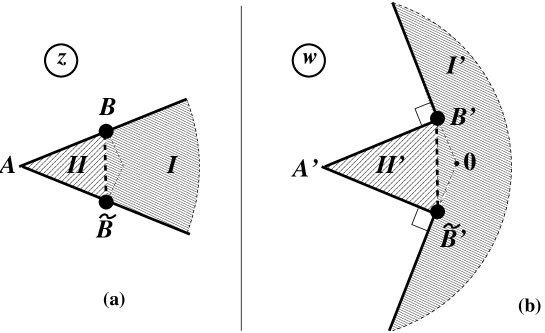
Figure 2: (a) The chart $\mathcal{M}_{z}^{(+)}$. Two boundary rays (solid lines) are identified. The dots indicate position of the zero of $p(z)$. (b) The image $\mathcal{M}_{w}^{(+)}$ of $\mathcal{M}_{z}^{(+)}$ under the map (5.7). The segment $A^{\prime}{\tilde{B}}^{\prime}$ is identified with $A^{\prime}B^{\prime}$, and the boundary line from ${\tilde{B}}^{\prime}$ to infinity is identified with the line from $B^{\prime}$ to infinity. Specific regions in this chart are discussed in the text.

In the new variables $(w,{\bar{w}})$ the solution ${\boldsymbol{\Xi}}(\rho,\phi\,|\,\theta)$ of the linear problem (1.10) can be written as

$${\boldsymbol{\Xi}}(\rho,\,\phi\,|\,\theta)=\exp\Big{[}\,{\textstyle{\sigma^{3}\over 4}\ \big{(}\,\mathrm{i}\pi+\log\big{(}{{\bar{p}}\over p}\big{)}\,\big{)}}\,\Big{]}\ {\hat{\boldsymbol{\Xi}}}\big{(}w,{\bar{w}}\,\,|\,\theta-{\textstyle\frac{\mathrm{i}\pi(\alpha+1)}{2\alpha}}\,\big{)}\ .$$ (5.10)

Here ${\hat{\boldsymbol{\Xi}}}(w,{\bar{w}}\,|\,\theta)$ is the solution of the linear problem

$$\Big{(}\partial_{w}+{\textstyle{1\over 2}}\ \partial_{w}{\hat{\eta}}\ \sigma^{3}-\mathrm{e}^{\theta}\ \ \ \big{[}\,\sigma^{+}\ \mathrm{e}^{{\hat{\eta}}}+\sigma^{-}\mathrm{e}^{-{\hat{\eta}}}\,\big{]}\,\Big{)}\ {\hat{\boldsymbol{\Xi}}}=0\ ,$$ (5.11)

$$\Big{(}\,{\partial}_{\bar{w}}-{\textstyle{1\over 2}}\ {\partial}_{\bar{w}}{\hat{\eta}}\ \sigma^{3}-\mathrm{e}^{-\theta}\big{[}\,\sigma^{-}\,\mathrm{e}^{{\hat{\eta}}}+\sigma^{+}\ \mathrm{e}^{-{\hat{\eta}}}\,\big{]}\,\Big{)}\ {\hat{\boldsymbol{\Xi}}}=0\ ,$$

associated with ShG equation (3.46), satisfying (for real $\theta$) the asymptotic condition,

$${\hat{\boldsymbol{\Xi}}}\to\begin{pmatrix}\ 1\\ -1\end{pmatrix}\ \ \exp\big{(}\,-w\,\mathrm{e}^{\theta}-{\bar{w}}\,\mathrm{e}^{-\theta}\,\big{)}\ \ \ \ \ \ {\rm as}\ \ \ w\in{\cal M}_{w}^{(+)}\to\infty\ .$$ (5.12)

Note that ${\hat{\boldsymbol{\Xi}}}(w,{\bar{w}}\,|\,\theta)$ is nothing but conventional Jost solution for (5.11) (see, e.g., [19] for details). The main advantage of the coordinates $(w,{\bar{w}})$ is relatively simple form of the large-$\theta$ asymptotic behavior of ${\hat{\boldsymbol{\Xi}}}$. Simple analysis of the linear problem (5.11) shows that

$${\hat{\boldsymbol{\Xi}}}(w,{\bar{w}}\,|\,\theta)\ \exp\big{(}\,w\,\mathrm{e}^{\theta}+{\bar{w}}\,\mathrm{e}^{-\theta}\,\big{)}\to\mathrm{e}^{\omega_{\pm}}\ \mathrm{e}^{\pm\frac{\hat{\eta}\sigma^{3}}{2}}\ \begin{pmatrix}\ 1\\ -1\end{pmatrix}\ \ \ {\rm as}\ \ \ \theta\to\pm\infty\,,$$ (5.13)

where $\omega_{\pm}=\omega_{\pm}(w,\,{\bar{w}})$ are local solutions of the Laplace equation $\partial_{w}\partial_{\bar{w}}\,\omega_{\pm}=0$ (in fact, $\omega_{\pm}$ are piecewise constants, see Eq.(5.22) below). Combining the difference equation (5.3) with the asymptotic behavior (5.13) and the analyticity condition for ${\hat{\boldsymbol{\Xi}}}$, it is straightforward to show that

$${\hat{\boldsymbol{\Xi}}}(w,{\bar{w}}\,|\,\theta)=\begin{pmatrix}\ \kappa_{+}X_{+}(w,{\bar{w}}\,|\,\theta)\\ -\kappa_{-}X_{-}(w,{\bar{w}}\,|\,\theta)\end{pmatrix}\ \ \exp\big{(}\,w\,\mathrm{e}^{\theta}+{\bar{w}}\,\mathrm{e}^{-\theta}\,\big{)}\ ,$$ (5.14)

where $\kappa_{\pm}=\kappa_{\pm}(w,{\bar{w}})$ do not depend on $\theta$, while $X_{\pm}$ are solutions of linear integral equations

$$X_{\pm}(w,{\bar{w}}\,|\,\theta)=1\pm\int_{-\infty}^{+\infty}{{\rm d}\theta^{\prime}\over 4\pi}\ \ \tanh\big{(}{\textstyle\frac{\theta-\theta^{\prime}}{2}}\big{)}\ D(w,{\bar{w}}\,|\,\theta^{\prime})\ X_{\pm}(w,{\bar{w}}\,|\,\theta^{\prime})$$ (5.15)

with the kernel

$$D(w,{\bar{w}}\,|\,\theta)=T_{\frac{1}{2}}\big{(}\theta+{\textstyle{\mathrm{i}\pi(\alpha+1)\over 2\alpha}}\big{)}\ \exp\big{(}-2w\,\mathrm{e}^{\theta}-2{\bar{w}}\,\mathrm{e}^{-\theta}\,\big{)}\ .$$ (5.16)

With Eqs.(5.13), (5.14) and

$$\det\Big{(}\,{\hat{\boldsymbol{\Xi}}}(w,{\bar{w}}\,|\,\theta+{\textstyle\frac{\mathrm{i}\pi}{2}}\big{)},\,\sigma^{3}\ {\hat{\boldsymbol{\Xi}}}(w,{\bar{w}}\,|\,\theta-{\textstyle\frac{\mathrm{i}\pi}{2}}\big{)}\,\Big{)}=2$$ (5.17)

one obtains

$$\kappa_{\pm}=d^{-\frac{1}{2}}\ \bigg{[}\,\frac{1-d_{-}^{2}}{1-d_{+}^{2}}\,\bigg{]}^{\pm\frac{1}{4}}\ ,$$ (5.18)

where

$$d_{\pm}=\int_{-\infty}^{+\infty}{{\rm d}\theta\over 4\pi}\ \ D(w,{\bar{w}}\,|\,\theta)\ X_{\pm}(w,{\bar{w}}\,|\,\theta)$$ (5.19)

and

$$d\equiv{\textstyle\frac{1}{2}}\ \Big{[}\,X_{+}\big{(}\theta+{\textstyle\frac{\mathrm{i}\pi}{2}}\big{)}X_{-}\big{(}\theta-{\textstyle\frac{\mathrm{i}\pi}{2}}\big{)}+X_{+}\big{(}\theta-{\textstyle\frac{\mathrm{i}\pi}{2}}\big{)}X_{-}\big{(}\theta+{\textstyle\frac{\mathrm{i}\pi}{2}}\big{)}\,\Big{]}=1-d_{+}d_{-}\ .$$ (5.20)

In these equations and below we omit the argument $(w,\bar{w})$ in $X_{\pm}$ and $d_{\pm}$, $\kappa_{\pm}$. Comparing the $\theta\to\pm\infty$ limits of (5.15) with (5.13), one can express the solution ${\hat{\eta}}$ of ShG equation (3.46) itself, as well as $\omega_{\pm}$, in terms of $d_{\pm}$,

$$\mathrm{e}^{2{\hat{\eta}}}=\frac{(1+d_{+})(1+d_{-})}{(1-d_{+})(1-d_{-})}$$ (5.21)

and

$$\mathrm{e}^{\omega_{\pm}}=1\pm\frac{d_{+}-d_{-}}{d}\ .$$ (5.22)

Note that the conjugation condition

$${\hat{\boldsymbol{\Xi}}}^{*}(w,{\bar{w}}\,|\,\theta)=-\sigma^{1}\ {\hat{\boldsymbol{\Xi}}}(w,{\bar{w}}\,|-\theta^{*})$$ (5.23)

implies the relations

$$X_{-}(w,{\bar{w}}\,|\,\theta)=X_{+}^{*}(w,{\bar{w}}\,|-\theta^{*})\ ,\ \ \ \ \ \ \ \kappa_{-}=\kappa_{+}^{*}\ ,$$ (5.24)

and hence

$$d_{-}=d_{+}^{*}\,,\ \ \ \ \ \ \ \ \ \ \ \ \ \ \omega_{-}=\omega_{+}^{*}\ .$$ (5.25)

Eq.(5.16) can be rewritten in the form

$$D(w,{\bar{w}}\,|\,\theta)=T^{(\rm reg)}_{\frac{1}{2}}\big{(}\theta+{\textstyle{\mathrm{i}\pi(\alpha+1)\over 2\alpha}}\big{)}\ \exp\big{(}-2w_{s}\,\mathrm{e}^{\theta}-2{\bar{w}}_{s}\,\mathrm{e}^{-\theta}\,\big{)}\ ,$$ (5.26)

where (see Eq.(5.9))

$$w_{s}(z)=\int^{z}_{s\mathrm{e}^{-\frac{\mathrm{i}\pi}{2\alpha}}}{\rm d}\zeta\ \sqrt{z^{2\alpha}+s^{2\alpha}}=w(z)+{\hat{r}}\ \tan\big{(}{\textstyle\frac{\pi}{2\alpha}}\big{)}-\mathrm{i}\ {\hat{r}}\ ,$$ (5.27)

and

$$T^{(\rm reg)}_{\frac{1}{2}}(\theta)=T_{\frac{1}{2}}(\theta)\ \exp\bigg{[}\,-{4\,{\hat{r}}\over\cos({\pi\over 2\alpha})}\,\cosh(\theta)\,\bigg{]}\ .$$ (5.28)

Advantage of using the function $T^{(\rm reg)}(\theta)$ is that it is well defined at any $\alpha>0$, including the points $\alpha^{-1}=1,\,3,\ldots$ , as opposed to both $Q_{\pm}(\theta)$ and $T(\theta)$, which at these points are defined only modulo overall factor $\exp(\,\text{const}\,\theta)$. Eq.(5.26) makes it explicit that the kernel of integral equations (5.15) is well defined at any $\alpha>0$, including the integer points. For example, in the case $\alpha=1$, it follows from Eqs.(3.36), (3.38), (4.19) and (5.28) that

$$T^{(\rm reg)}_{\frac{1}{2}}(\theta) = \exp\bigg{\{}\,\int_{-\infty}^{\infty}\frac{{\rm d}t}{2\pi\cosh(\theta-t)}\times$$

$$\log\Big{[}\,\big{(}1+\mathrm{e}^{-\pi s^{2}\cosh(t)+2\pi\mathrm{i}k}\,\big{)}\,\big{(}1+\mathrm{e}^{-\pi s^{2}\cosh(t)-2\pi\mathrm{i}k}\,\big{)}\,\Big{]}\,\bigg{\}}\ .$$

For $k={1\over 4}$ this function, interpreted as a Stokes coefficient, was found in Ref.[14]. This result was also used in Ref.[16].

Eqs.(5.26)-(5.28) and (4.20) imply that for

$$\Re e\,(w)>-{\hat{r}}\ \tan\big{(}{\textstyle\frac{\pi}{2\alpha}}\big{)}\ ,$$ (5.30)

and real $\theta$ the kernel $|D(w,{\bar{w}}\,|\theta)|$ is bounded by $\exp\big{(}-C\ \cosh(\theta)\big{)}$ with positive constant $C$. In this domain of $w$ the integral equations (5.15) have unique solutions obtainable by iterations. With appropriate deformation of the integration contours in  (5.15) one can extend the domain of applicability of the iterative solution to the region $I^{\prime}\subset{\cal M}_{w}^{(+)}$ shown in Fig.2b. The most efficient way to solve (5.15) at the boundary of $I^{\prime}$, i.e. on the segment $\Re e\,(w)=-{\hat{r}}\ \tan\big{(}{\textstyle\frac{\pi}{2\alpha}}\big{)}$, $\big{|}\Im m\,(w)\big{|}<{\hat{r}}$, is based on the integral transformation in $\lambda=\mathrm{e}^{\theta}$ generated by the kernel $\exp\big{(}\,\mathrm{i}\xi\,(\lambda-\lambda^{-1})\,\big{)}$. The transformation brings (5.15) into the form of Gel’fand-Levitan-Marchenko equation (see e.g. [19] for details). Important problem of reconstruction of the Jost solution ${\hat{\boldsymbol{\Xi}}}(w,\,{\bar{w}}\,|\,\theta)$ in the whole domain ${\cal M}_{w}^{(+)}$ is beyond the scope of this paper.

5.2 Solution of MShG equation

Since ${\hat{\eta}}$ decays at $|w|\to\infty$, at large $|w|$ it approaches certain solution ${\hat{\eta}}_{1}$ of the linearized equation $\partial_{w}\partial_{{\bar{w}}}\,{\hat{\eta}}_{1}-4\,{\hat{\eta}}_{1}=0$. The form of this solution can be read out from Eq.(5.21),

$${\hat{\eta}}_{1}=\int_{-\infty}^{\infty}\frac{{\rm d}\theta}{2\pi}\ T_{\frac{1}{2}}\big{(}\theta+{\textstyle{\mathrm{i}\pi(\alpha+1)\over 2\alpha}}\big{)}\ \exp\big{(}-2w\,\mathrm{e}^{\theta}-2{\bar{w}}\,\mathrm{e}^{-\theta}\,\big{)}\ .$$ (5.31)

Furthermore, iterations of (5.15) produce (through (5.19), (5.20), and (5.21)) systematic large-$|w|$ expansion of ${\hat{\eta}}$. In fact, one can guess the form of this expansion without explicit calculations. As is known [43],[3], the series

$${\hat{\eta}}=\sum_{n=1}^{\infty}\,{\hat{\eta}}_{2n-1}\,,$$ (5.32)

$${\hat{\eta}}_{2n-1}={2\over 2n-1}\ \ \int_{-\infty}^{\infty}\prod_{j=1}^{2n-1}\bigg{[}\,\frac{{\rm d}\theta_{j}}{4\pi}\ \frac{{\cal T}(\theta_{j})\,\exp\big{(}-2w\,\mathrm{e}^{\theta}-2{\bar{w}}\,\mathrm{e}^{-\theta}\,\big{)}}{\cosh\big{(}{\theta_{j}-\theta_{j+1}\over 2}\big{)}}\,\bigg{]}\ ,$$

with $\theta_{2n}\equiv\theta_{1}$, and arbitrary function ${\cal T}(\theta)$, provides formal solution of the ShG equation (3.46). Since the asymptotic form (5.21) fixes the solution uniquely, we conclude that the solution ${\hat{\eta}}$ we are interested in is given (in certain domain of $w$ specified below) by the series (5.32) with

$${\cal T}(\theta)=T_{\frac{1}{2}}\big{(}\theta+{\textstyle{\mathrm{i}\pi(\alpha+1)\over 2\alpha}}\big{)}\ .$$ (5.33)

This representation is very useful since at sufficiently large $w$ the series (5.32) converges fast. In view of Eq.(4.20), the multiple integrals in (5.32) converge only when $w$ belongs to the domain (5.30). With deformation of the integration contours, the convergence domain can be extended to $I^{\prime}\subset{\cal M}_{w}^{(+)}$ shown in Fig.2b. Thus, the solution of MShG (1.5) in the domain $I\subset{\cal M}_{z}^{(+)}$ (Fig.2a) can be written in the form $\eta={\hat{\eta}}+\frac{1}{4}\ \log(p{\bar{p}})$, where ${\hat{\eta}}$ and $p$ are given by (5.32) and (5.6), respectively. It would be interesting to find similarly explicit expression for ${\hat{\eta}}$ in the remaining part of ${\cal M}_{z}^{(+)}$.

As $|w|\to\infty$, the integral (5.31) can be evaluated by the saddle-point method. As the result one derives the large-$\rho$ asymptotic of the solution of MShG (1.5), (1.6),

$$\eta(\rho,\phi) \to {\textstyle\frac{1}{4}}\ \log\big{(}\,s^{4\alpha}-2\,(s\rho)^{2\alpha}\,\cos(2\alpha\phi)+\rho^{4\alpha}\,\big{)}$$

$$+ T_{\frac{1}{2}}\big{(}\,\mathrm{i}(\alpha+1)\phi\,\big{)}\ {\mathrm{e}^{-\tau}\over\sqrt{2\pi\tau}}\ \Big{(}\,1+O(\tau^{-1})\,\Big{)}\ \ \ {\rm as}\ \ \tau={\textstyle\frac{4\rho^{\alpha+1}}{\alpha+1}}\to+\infty\ .$$

In writing this equation we use the original polar coordinates $(\rho,\,\phi)$ on the chart ${\cal M}_{z}^{(0)}$ (2.6), and assume for simplicity that $\alpha>1$. Eq.(5.2) shows that the $T$-function $T_{\frac{1}{2}}(\theta)$ determines the angular dependence of the sub-leading large-$\rho$ asymptotic of the MShG solution. At $s=0$ and finite $\theta$ the function $T_{\frac{1}{2}}(\theta)$ becomes a constant,

$$T_{\frac{1}{2}}(\theta)\big{|}_{s=0}=2\ \cos\big{(}{\textstyle\frac{\pi(2l+1)}{2(\alpha+1)}}\big{)}\ ,$$ (5.35)

and hence (5.2) generalizes the well known asymptotic formula for the Painlevé III transcendent [43].

6 MShG with $\alpha<-1$ and quantum sinh-Gordon model

So far we were concentrating attention on MShG with $\alpha>0$. In that case we had a freedom to adjust the asymptotic behavior of $\eta$ at $z\to 0$ as in (2.5), with the free parameter $l$. If $\alpha<-1$, the situation is different: asymptotic form of a regular solution is fixed at both $z\to\infty$ and $z\to 0$. In fact, the roles of $z=0$ and $z=\infty$ can be interchanged by certain “duality” transformation. Conformal transformation

$${\tilde{z}}=\left[-\,\frac{s^{\alpha}\,z}{\alpha+1}\,\right]^{\alpha+1}$$ (6.1)

(with suitable shift of the field $\eta$) brings the MShG equation to the original form, but with the parameters $\alpha,s$ replaced by the “dual” values ${\tilde{\alpha}},\ {\tilde{s}}$ related to the original ones as

$$(\alpha+1)\,({\tilde{\alpha}}+1)=1\,,\qquad\qquad\qquad{\tilde{s}}^{{\tilde{\alpha}}+1}=-\frac{s^{\alpha+1}}{\alpha+1}\ .$$ (6.2)

Note that in terms of the parameters $b$ and $\mu$, Eq.(1.12), these relations faithfully reproduce the $b\to b^{-1}$ duality symmetry of the quantum sinh-Gordon model [44]. Below we argue that such solution (more precisely, certain connection coefficient for solutions of the linear problem (1.10)) is related to the $Q$-function of the sinh-Gordon model (1.13).

In this discussion we will use the chart ${\cal M}^{(+)}_{z}$ on ${\mathbb{C}}_{\frac{\pi}{\nu}}$, in which $p(z)$ has the form (5.6), and associated polar coordinates $z=\rho\exp({i\phi})$. We also use the notation

$$\nu=-{\alpha}\ .$$ (6.3)

We assume that MShG equation has solution $\eta(\rho,\phi)$ which is real and continuous on ${\mathbb{C}}_{\frac{\pi}{\nu}}$ except for the apex $\rho=0$, and has the following properties (compare to the properties ${\bf i})-{\bf iv})$ in Section 2)

${\bf i}^{\prime})$

$$\eta\big{(}\rho,\phi+{\textstyle\frac{\pi}{\nu}}\big{)}=\eta(\rho,\phi)\,.$$ (6.4)

${\bf ii}^{\prime})$ $\eta(\rho,\phi)$ are real-valued and finite everywhere on the cone $\mathbb{C}_{\frac{\pi}{\alpha}}$, except for the apex $\rho=0$.

${\bf iii}^{\prime})$

$$\eta(\rho,\phi)\to 0\ \ \ \ \ \ \ \ {\rm as}\ \ \ \ \rho\to\infty\ .$$ (6.5)

${\bf iv}^{\prime})$

$$\eta(\rho,\phi)\to-\nu\ \log(\rho)+O(1)\ \ \ \ \ \ \ \ {\rm as}\ \ \ \ \rho\to 0\ .$$ (6.6)

The relevant linear problem (1.10) now is somewhat simpler then that previously discussed. At $\nu>1$ we introduce two solutions of the linear problem, defined by the asymptotic conditions at $\rho\to\infty$ and $\rho\to 0$,

$${{\boldsymbol{\Xi}}}_{+}(\rho,\,\phi\,|\,\theta)\to\begin{pmatrix}1\\ -1\end{pmatrix}\ \exp\Big{[}-2s^{-\nu}\ \rho\ \cosh(\theta+\mathrm{i}\phi)\,\Big{]}\ \ \ \ \ \ {\rm as}\ \ \ \rho\to+\infty\ ,$$ (6.7)

and

$${{\boldsymbol{\Xi}}}_{-}(\rho,\,\phi\,|\,\theta)\to\begin{pmatrix}\mathrm{e}^{-{\mathrm{i}\nu\phi\over 2}}\\ \mathrm{e}^{{\mathrm{i}\nu\phi\over 2}}\end{pmatrix}\ \exp\bigg{[}\,-{2\rho^{1-\nu}\over\nu-1}\ \cosh(\theta-\mathrm{i}(\nu-1)\phi\big{)}\,\bigg{]}\ \ \ \ \ \ {\rm as}\ \ \ \rho\to 0\ .$$ (6.8)

We then define

$${\cal Q}(\theta)={\textstyle{1\over 2}}\ \det\big{(}{{\boldsymbol{\Xi}}}_{+},\,{{\boldsymbol{\Xi}}}_{-}\big{)}\ .$$ (6.9)

By arguments parallel to the analysis in [44, 45], it is possible to establish the following properties of this connection coefficient:

• ${\cal Q}(\theta)$ is an entire function of $\theta$ with the symmetries

  $${\cal Q}(\theta)={\cal Q}(-\theta)\ ,\ \ \ \ \ \ \ {\cal Q}^{*}(\theta)={\cal Q}(\theta^{*})\ .$$ (6.10)

• ${\cal Q}(\theta)$ satisfies the Quantum Wronskian relation:

  $${\cal Q}\big{(}\theta-{\textstyle{{\rm i}\pi\over 2}}\big{)}{\cal Q}\big{(}\theta+{\textstyle{{\rm i}\pi\over 2}}\big{)}-{\cal Q}\big{(}\theta+{\textstyle{{\rm i}\pi(\nu-2)\over 2\nu}}\big{)}{\cal Q}\big{(}\theta-{\textstyle{{\rm i}\pi(\nu-2)\over 2\nu}}\big{)}=1\ .$$ (6.11)

• As the function of the complex $\theta$, ${\cal Q}(\theta)$ is free of zeroes in the strip $\big{|}\Im m\,\theta\big{|}<{\pi\over 2}+\epsilon$ for some finite $\epsilon>0$.

• For $\big{|}\Im m\,\theta\big{|}<{\pi\over 2}+\epsilon$ and $\Re e\,\theta\to+\infty$

  $${\cal Q}(\theta)=\exp\bigg{[}-{{2\ {\hat{r}}\over\sin({\pi\over\nu})}}\ \mathrm{e}^{\theta}+O(\mathrm{e}^{-\theta})\,\bigg{]}\ ,$$ (6.12)

  where

  $${\hat{r}}={\pi^{3\over 2}\ \nu\over(\nu-1)\Gamma({1\over 2\nu})\Gamma({\nu-1\over 2\nu})}\ s^{1-\nu}\ .$$ (6.13)

Let us introduce the function $\varepsilon(\theta)$ through the relation

$${\cal Q}\big{(}\theta+{\textstyle{{\rm i}\pi\over 2}}\big{)}\,{\cal Q}\big{(}\theta-{\textstyle{{\rm i}\pi\over 2}}\big{)}=1+\mathrm{e}^{-\varepsilon(\theta)}\ .$$ (6.14)

With the analytic properties listed above, it is straightforward to transform the difference equation (6.11) into integral equation for $\varepsilon(\theta)$ (see Ref.[27]),

$$\varepsilon(\theta)-8\,{\hat{r}}\ \cosh(\theta)+\int_{-\infty}^{\infty}{{\rm d}\theta^{\prime}\over 2\pi}\ \Phi(\theta-\theta^{\prime})\ \log\big{(}1+\mathrm{e}^{-\varepsilon(\theta^{\prime})}\,\big{)}$$ (6.15)

with the kernel

$$\Phi(\theta)={4\,\sin({\pi\over\nu})\ \cosh(\theta)\over\cosh(2\theta)-\cos({2\pi\over\nu})}\ .$$ (6.16)

Then

$$\log{\cal Q}(\theta)=-{4\,{\hat{r}}\over\sin({\pi\over\nu})}\ \cosh(\theta)+\int_{-\infty}^{\infty}{{\rm d}\theta^{\prime}\over 2\pi}\ {\log\big{(}1+\mathrm{e}^{-\varepsilon(\theta^{\prime})}\big{)}\over\cosh(\theta-\theta^{\prime})}\ .$$ (6.17)

As was argued in Ref.[28], Eq.(6.17) gives the $Q$-function for the quantum sinh-Gordon model in the finite-size geometry (1.3), provided ${\hat{r}}=\frac{mR}{8}$, with $m$ interpreted as the mass of the sinh-Gordon particle, and $\nu$ related to the sinh-Gordon coupling constant $b$ as in (1.12), i.e.

$$\nu=b^{-2}+1\ .$$ (6.18)

It is instructive to review the above statements in terms of the coordinate

$$w=w(z)=\int{\rm d}z\ \sqrt{z^{-2\nu}+s^{-2\nu}}$$ (6.19)

which brings the MShG equation to the form of the conventional ShG equation (3.46) for ${\hat{\eta}}=\eta-\frac{1}{4}\,\log(p{\bar{p}})$. We fix the integration constant in (6.19) in such a way that

$$w\big{(}\,s\,\mathrm{e}^{\pm\mathrm{i}{\pi\over 2\nu}}\,\big{)}=\pm\mathrm{i}\,{\hat{r}}\ .$$ (6.20)

Explicitly,

$$w(z)=-{\hat{r}}\ \cot\big{(}{\textstyle{\pi\over 2\nu}}\big{)}+z\,s^{-\nu}\ {}_{2}F_{1}\big{(}-{\textstyle{1\over 2}},\,-{\textstyle{1\over 2\nu}},\,1-{\textstyle{1\over 2\nu}},-\big{(}{\textstyle{z\over s}}\big{)}^{-2\nu}\ \big{)}\ .$$ (6.21)

The chart ${\cal M}^{(+)}_{z}$ and its $w$-image ${\cal M}^{(+)}_{w}$ are shown in Fig.3a and Fig.3b.

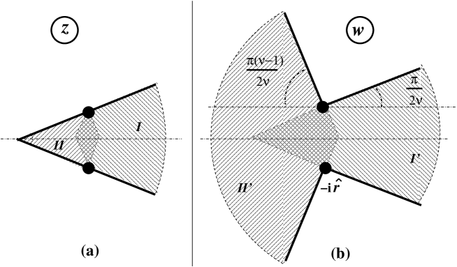
Figure 3: The chart $\mathcal{M}_{z}^{(+)}$ (a), and its image $\mathcal{M}_{w}^{(+)}$ under the map (6.21) (b) in the case $\nu=-\alpha>0$.

The asymptotic conditions ${\bf iii}^{\prime})$ and ${\bf iv}^{\prime})$ above simply mean that ${\hat{\eta}}$ decays at $|w|\to\infty$ in both regions $I^{\prime}$ and $II^{\prime}$ in Fig.3b. Eq.(6.9) can be equivalently written as

$${\cal Q}(\theta)={{1\over 2}}\ \exp\bigg{[}-{{4\,{\hat{r}}\over\sin({\pi\over\nu})}}\ \cosh(\theta)\,\bigg{]}\ \ \det\big{(}\,{\hat{\boldsymbol{\Xi}}}_{+},\,{\hat{\boldsymbol{\Xi}}}_{-}\big{)}\ ,$$ (6.22)

where ${\hat{\boldsymbol{\Xi}}}_{\pm}$ are conventional Jost solutions [19] for the linear problem (5.11) satisfying the asymptotic conditions

$${\hat{\boldsymbol{\Xi}}}_{+}(w,{\bar{w}}\,|\,\theta)\to\exp\big{(}-w\,\mathrm{e}^{\theta}-{\bar{w}}\,\mathrm{e}^{-\theta}\,\big{)}\ \begin{pmatrix}1\\ -1\end{pmatrix}\ \ \ \ \ \ {\rm as}\ \ \ \Re e(w)\to+\infty\ ,$$ (6.23)

and

$${\hat{\boldsymbol{\Xi}}}_{-}(w,{\bar{w}}\,|\,\theta)\to\exp\big{(}\,w\,\mathrm{e}^{\theta}+{\bar{w}}\,\mathrm{e}^{-\theta}\,\big{)}\ \begin{pmatrix}1\\ 1\end{pmatrix}\ \ \ \ \ \ {\rm as}\ \ \ \Re e(w)\to-\infty\ .$$ (6.24)

In this picture the duality (6.1) is quite evident. The rotation $w\to-w$ interchanges domains $I^{\prime}$ and $II^{\prime}$ in Fig.3b , which is equivalent to the change of the parameters

$$\nu^{-1}\to 1-\nu^{-1}\ ,\qquad{\hat{r}}\to{\hat{r}}$$ (6.25)

identical to (6.2) (Note that (6.13) is invariant under the transformation (6.2)). It is easy to check that under this duality

$${\hat{\boldsymbol{\Xi}}}_{\pm}(w,{\bar{w}}\,|\,\theta)\leftrightarrow\sigma^{3}\ {\hat{\boldsymbol{\Xi}}}_{\mp}(-w,-{\bar{w}}\,|\,\theta)\ ,$$ (6.26)

and hence the function ${\cal Q}(\theta)$ does not change when its parameters are transformed as in (6.25). Thus, it is invariant with respect to the $b\to b^{-1}$ duality, as the sinh-Gordon $Q$-function should be.

The asymptotic expansions at $\theta\to+\infty$ and $\theta\to-\infty$ of ${\cal Q}(\theta)$ generate the vacuum eigenvalues of the local integral of motions in the quantum sinh-Gordon model. Namely [28],

$$\log{\cal Q}\sim-C_{0}\ \mathrm{e}^{\theta}-\sum_{n=1}^{\infty}C_{n}\,I_{2n-1}\ \mathrm{e}^{-(2n-1)\theta}\ \ \ \ {\rm as}\ \ \ \ \ \theta\to+\infty\ ,$$ (6.27)

$$\log{\cal Q}\sim-C_{0}\ \mathrm{e}^{-\theta}-\sum_{n=1}^{\infty}C_{n}\,{\bar{I}}_{2n-1}\ \mathrm{e}^{(2n-1)\theta}\ \ \ \ {\rm as}\ \ \ \ \ \theta\to-\infty\ ,$$

where $I_{2n-1}$ and ${\bar{I}}_{2n-1}$ are the vacuum eigenvalues of the local integral of motions ${\mathbb{I}}_{2n-1}$ and ${\bar{\mathbb{I}}}_{2n-1}$ $(n=1,\,2,\,\ldots)$ normalized as in (3.59). The constant $C_{n}$ are given by (3.63) with $\alpha=-\nu$, where $m$ is interpreted as the mass of the sinh-Gordon particle. From Eq.(6.17) we have

$$C_{n}\ I_{2n-1} = C_{0}\ \delta_{n,1}+(-1)^{n}\ \int_{-\infty}^{\infty}{{\rm d}\theta\over\pi}\ \mathrm{e}^{(2n-1)\theta}\ \log\Big{(}1+\mathrm{e}^{-\varepsilon(\theta)}\,\Big{)}\ ,$$ (6.28)

$$C_{n}\ {\bar{I}}_{2n-1} = C_{0}\ \delta_{n,1}+(-1)^{n}\ \int_{-\infty}^{\infty}{{\rm d}\theta\over\pi}\ \mathrm{e}^{-(2n-1)\theta}\ \log\Big{(}1+\mathrm{e}^{-\varepsilon(\theta)}\,\Big{)}\ .$$

On the other hand, straightforward WKB analysis allows one to express (6.28) in terms of the classical conserved charges for MShG equation,

$$C_{n}\ I_{2n-1} = {(-1)^{n}\over 2n-1}\ \int_{-\infty}^{\infty}\Big{[}\,{\rm d}w\ {\hat{P}}_{2n}+{\rm d}{\bar{w}}\ {\hat{R}}_{2n-2}\,\Big{]}\ ,$$ (6.29)

$$C_{n}\ {\bar{I}}_{2n-1} = {(-1)^{n}\over 2n-1}\ \int_{-\infty}^{\infty}\Big{[}\,{\rm d}{\bar{w}}\ {\hat{\bar{P}}}_{2n}+{\rm d}{w}\ {\hat{\bar{R}}}_{2n-2}\,\Big{]}\ .$$

Further analysis is similar to the one presented in Section 5 for $\alpha>0$. The novel property is existence of two Jost solutions. For this reason one has to introduce two $T$-functions ${\cal T}_{\pm}$,

$${\cal T}_{+}(\theta)\ {\cal Q}(\theta) = {\cal Q}\big{(}\theta+{\textstyle{\mathrm{i}\pi\over\nu}}\big{)}+{\cal Q}\big{(}\theta-{\textstyle{\mathrm{i}\pi\over\nu}}\big{)}\ ,$$ (6.30)

$${\cal T}_{-}(\theta)\ {\cal Q}(\theta) = {\cal Q}\big{(}\theta+{\textstyle{\mathrm{i}(\nu-1)\pi\over\nu}}\big{)}+{\cal Q}\big{(}\theta-{\textstyle{\mathrm{i}\pi(\nu-1)\over\nu}}\big{)}\ .$$

Note that the duality transformation (6.25) interchanges the $T$-functions,

$${\cal T}_{\pm}(\theta)\leftrightarrow{\cal T}_{\mp}(\theta)\ .$$ (6.31)

The ShG solution ${\hat{\eta}}$ still can be written as the series (5.32), but the choice of the function ${\cal T}(\theta)$ is different for the two parts $I^{\prime}$ and $II^{\prime}$ of the chart ${\cal M}^{(+)}_{w}$ in Fig.3b. Thus, for $w\in I^{\prime}$ we have

$${\hat{\eta}}=\sum_{n=1}^{\infty}\,\,{2\over 2n-1}\ \ \int_{-\infty}^{\infty}\prod_{j=1}^{2n-1}\bigg{[}\,\frac{{\rm d}\theta_{j}}{4\pi}\ \frac{{\cal T}_{+}(\theta_{j})\,\exp\big{(}-2w_{+}\,\mathrm{e}^{\theta}-2{\bar{w}_{+}}\,\mathrm{e}^{-\theta}\,\big{)}}{\cosh\big{(}{\theta_{j}-\theta_{j+1}\over 2}\big{)}}\,\bigg{]}\ ,$$ (6.32)

where

$$w_{+}={\hat{r}}\ \cot\big{(}{\textstyle{\pi\over 2\nu}}\big{)}+w\ .$$ (6.33)

For $w\in II^{\prime}$ one has to replace ${\cal T}_{+}(\theta)$ by ${\cal T}_{-}(\theta)$, and $w_{+}$ by

$$w_{-}=-{\hat{r}}\ \tan\big{(}{\textstyle{\pi\over 2\nu}}\big{)}-w\ .$$ (6.34)

Since the union $I^{\prime}\cup II^{\prime}$ covers the whole chart ${\cal M}^{(+)}_{w}$, combination of these two representations provide the solution $\eta$ on the whole cone ${\mathbb{C}}_{\frac{\pi}{\nu}}$.

7 Discussion

In this paper we have described relation between the classical MShG equation and its linear problem, on one hand, and quantum sine- and sinh-Gordon models on the other. This relation generalizes the relation [20, 26] between ordinary differential equations [24, 25] and integrable structures of Conformal Field Theories [21, 22, 23] to the massive case. We believe it also brings useful insight into the emergence of TBA equations in recent analysis of the MShG equation [14, 15, 16, 17, 18].

The discussion in this paper is in terms of the $Q$- and $T$-functions of the quantum models (1.2) and (1.13), which are defined through the Bethe Ansatz for the vacuum states. More generally, these functions have to be understood as the vacuum eigenvalues one-parameter families of commuting operators $\mathbb{Q}(\theta)$ and $\mathbb{T}(\theta)$. In integrable lattice models (e.g. XXZ and XYZ chains) these operators were discovered in pioneering works of Baxter [32, 33]. When an integrable quantum field theory emerges as continuous (scaling) limit of such lattice systems, it inherits these operators. However, for many reasons (including subtleties of the continuous limit) it is desirable to have constructions of these operators directly in field theoretic terms. There was some progress in this direction. Thus, in Ref.[21] the operators $\mathbb{T}_{j}(\theta),\ j=\frac{1}{2},\,1,\,\frac{3}{2},\,\ldots$ were constructed explicitly for massless (conformal) field theory, as traces of quantum monodromy matrices over $2j+1$ dimensional auxiliary spaces. This construction of $\mathbb{T}_{j}(\theta)$ admits more or less direct extension to the massive sine-Gordon model and its reductions [41]. In both massless and massive cases it allows one to establish directly basic properties of these operators, which we summarize in Appendix B. In particular, one can argue that all $\mathbb{T}_{j}(\theta)$ are entire functions of $\theta$, in the sense that all their simultaneous eigenvalues are entire functions. Furthermore, in the massless case similar construction (with auxiliary space supporting representation of $q$-oscillator algebra) exists for the $Q$-operator [22, 23]. It is plausible that it also admits generalization to the massive case, but the details were never elaborated. However, both the massless construction and the lattice theory suggest certain properties of the sine-Gordon $Q$-operator. Thus, one expects that $\mathbb{Q}(\theta)$ is entire function of $\theta$ as well. This operator commutes with all $\mathbb{T}_{j}(\theta^{\prime})$, and satisfies the famous $T-Q$ equation of Baxter,

$${\mathbb{T}}_{\frac{1}{2}}(\theta)\ {\mathbb{Q}}(\theta)={\mathbb{Q}}\big{(}\theta+{\textstyle\frac{\mathrm{i}\pi}{\alpha}}\big{)}+{\mathbb{Q}}\big{(}\theta+{\textstyle\frac{\mathrm{i}\pi}{\alpha}}\big{)}\ ,$$ (7.1)

familiar from the lattice theory [32, 33]. This equation is finite difference analog of a second order differential equation. Since in the sine-Gordon model $\mathbb{T}(\theta)$ is periodic function of $\theta$ (see Eq.(B.7)), one expects to have two “Bloch wave” solutions $\mathbb{Q}_{\pm}(\theta)$,

$${\mathbb{Q}}_{+}\big{(}\theta+{\textstyle\frac{\mathrm{i}\pi(\alpha+1)}{\alpha}}\big{)}={\mathbb{U}}\ {\mathbb{Q}}_{+}(\theta)\ ,$$ (7.2)

$${\mathbb{Q}}_{-}\big{(}\theta+{\textstyle\frac{\mathrm{i}\pi(\alpha+1)}{\alpha}}\big{)}={\mathbb{U}}^{-1}\ {\mathbb{Q}}_{-}(\theta)\ ,$$

with some unitary operator $\mathbb{U}$ commuting with $\mathbb{Q}_{\pm}(\theta)$. Again, by comparison to the massless limit [22, 23, 41], it is natural to identify $\mathbb{U}$ with the Flouquet-Bloch operator associated with the discrete symmetry of the sine-Gordon theory,

$${\mathbb{U}}\,\varphi(x,t)\,{\mathbb{U}}^{-1}=\varphi(x,t)+2\pi/\beta\ .$$ (7.3)

Since $\mathbb{T}_{\frac{1}{2}}(\theta)$ is invariant with respect to the charge conjugation (B.1), the operators $\mathbb{Q}_{+}(\theta)$ and $\mathbb{Q}_{-}(\theta)$ are related to each other by this symmetry transformation, Eq.(B.13) (this symmetry was already taken into account in writing (7.2)), so one can deal with one independent operator, say $\mathbb{Q}\equiv\mathbb{Q}_{+}$. Additional piece of analytic information – the asymptotic behavior

$$\log\mathbb{Q}(\theta)\sim\text{const}\ \mathrm{e}^{\pm\theta}+O(1)$$ (7.4)

as $\Re e(\theta)\to\pm\infty$ in the strips $H_{\pm}$ (3.10) – can be inferred from the massless $Q$-operators [22, 23]. These assumptions and some of their simple consequences (in particular, precise form of (7.4)) are summarized in Appendix B.

Once the sine-Gordon $Q$-function $Q(\theta,k)$ is understood as the $k$-vacuum eigenvalue of the $Q$-operator, the question arises about its eigenvalues associated with the excited states. Basic properties of such eigenvalues can be inferred from (B.10)-(B.15). Can the excited-state eigenvalues be also related to integrable classical equations? In the massless case it is known how to modify the Schr${\rm\ddot{o}}$dinger equation (2.31) to accommodate for the excited states [31]. In the massive theory this is interesting open question. Of course, generalization of the DDV equation (3.32) to the excited states is well known [10, 46].

Appendix

Appendix A Derivation of Eqs.(3.1)-(3.4)

Here we sketch derivation of the properties (3.1)-(3.4) of $Q_{\pm}$.

Eqs.(3.2) follow from (2.19),  (2.20) and easily established relation

$$\sigma^{1}\,{\boldsymbol{\Xi}}^{*}(\rho,\phi\,|-\theta)=-{\boldsymbol{\Xi}}(\rho,\phi\,|\,\theta)\qquad\text{at}\quad\Im m(\theta)=0\ .$$ (A.1)

To prove the quasiperiodicity (3.1) we use the evident relation

$$Q_{-}(\theta)=W\ \det\Big{[}\,{\boldsymbol{\Xi}}(\rho,\phi\,|\,\theta),\,{\boldsymbol{\Psi}}_{-}(\rho,\phi\,|\,\theta)\,\Big{]}\ ,$$ (A.2)

where $W=-\cos(\pi l)$. Then

$$Q_{-}\big{(}\theta-{\textstyle{\mathrm{i}\pi(\alpha+1)\over 2\alpha}}\big{)}=W\times$$ (A.3)

$$\det\Big{[}\,{\boldsymbol{\Xi}}\big{(}\rho,\phi+{\textstyle{\pi\over 2\alpha}}\,|\,\theta-{\textstyle{\mathrm{i}\pi(\alpha+1)\over 2\alpha}}\,\big{)}\,,\,{\boldsymbol{\Psi}}_{-}\big{(}\rho,\phi+{\textstyle{\pi\over 2\alpha}}\,|\,\theta-{\textstyle{\mathrm{i}\pi(\alpha+1)\over 2\alpha}}\,\big{)}\,\Big{]}\ .$$

The following formula is immediate consequence of Eqs.(2.16), (2.17),

$${\boldsymbol{\Psi}}_{-}\big{(}\rho,\phi+{\textstyle{\pi\over\alpha}}\,|\,\theta-{\textstyle{\mathrm{i}\pi(\alpha+1)\over\alpha}}\,\big{)}=\mathrm{e}^{\mathrm{i}\pi l}\ \sigma^{3}\ {\boldsymbol{\Psi}}_{-}(\rho,\phi\,|\,\theta)\ .$$ (A.4)

It is also straightforward to prove similar relation for the solution ${\boldsymbol{\Xi}}$,

$${\boldsymbol{\Xi}}\big{(}\rho,\phi+{\textstyle{\pi\over\alpha}}\,|\,\theta-{\textstyle{\mathrm{i}\pi(\alpha+1)\over\alpha}}\,\big{)}=-\mathrm{i}\,\sigma^{3}\ {\boldsymbol{\Xi}}(\rho,\phi\,|\,\theta)\ .$$ (A.5)

Using (A.4) and (A.5) one has

$$Q_{-}\big{(}\theta-{\textstyle{\mathrm{i}\pi(\alpha+1)\over 2\alpha}}\,\big{)}=-\mathrm{i}\,\mathrm{e}^{\mathrm{i}\pi l}\ W\times$$ (A.6)

$$\det\Big{[}\,\sigma^{3}\,{\boldsymbol{\Xi}}\big{(}\rho,\phi+{\textstyle{\pi\over 2\alpha}}\,|\,\theta-{\textstyle{\mathrm{i}\pi(\alpha+1)\over 2\alpha}}\,\big{)}\,,\,\sigma^{3}\,{\boldsymbol{\Psi}}_{-}\big{(}\rho,\phi-{\textstyle{\pi\over 2\alpha}}\,|\,\theta+{\textstyle{\mathrm{i}\pi(\alpha+1)\over 2\alpha}}\,\big{)}\,\Big{]}$$

$$\ \ \ \ \ \ \ \ \ \ \ \ \ \ \ \ \ \ \ \ \ \ =\mathrm{i}\,\mathrm{e}^{\mathrm{i}\pi l}\ Q_{-}\big{(}\theta+{\textstyle{\mathrm{i}(\alpha+1)\pi\over 2\alpha}}\,\big{)}\ .$$

For given values of $\rho$ and $\phi$, the solution ${\boldsymbol{\Xi}}$ (2.23), considered as the function of complex $\theta$, is analytic in the strip $-{\textstyle{\pi\over 2}}-(\alpha+1)\,\phi\leq\Im m(\theta)\leq{\textstyle{\pi\over 2}}-(\alpha+1)\,\phi$. Since ${\boldsymbol{\Psi}}_{-}$ is entire function of $\theta$, one concludes that $Q_{+}(\theta)$ is analytic in the strip $|\Im m(\theta)|<\pi+{\pi\over 2\alpha}$, and hence due to the quasiperiodicity (3.1) it is entire function of $\theta$. Since $Q_{\pm}$ and ${\boldsymbol{\Psi}}_{\pm}$ are entire functions of $\theta$,   ${\boldsymbol{\Xi}}$ (2.25) is an entire function as well.

To prove the Quantum Wronskian relation (3.3) we use (2.25) to obtain

$${\boldsymbol{\Xi}}(\rho,\phi\mp{\textstyle{\pi\over 2\alpha}}\,|\,\theta\pm{\textstyle{\mathrm{i}\pi\over 2\alpha}}) = Q_{-}(\theta\pm{\textstyle{\mathrm{i}\pi\over 2\alpha}})\ {\boldsymbol{\Psi}}_{+}(\rho,\phi\mp{\textstyle{\pi\over 2\alpha}}\,|\,\theta\pm{\textstyle{\mathrm{i}\pi\over 2\alpha}})$$ (A.7)

$$+ Q_{+}(\theta\pm{\textstyle{\pi\over 2\alpha}})\ {\boldsymbol{\Psi}}_{-}(\rho,\phi\mp{\textstyle{\pi\over 2\alpha}}\,|\,\theta\pm{\textstyle{\mathrm{i}\pi\over 2\alpha}})\ .$$

From (2.16) we have

$${\boldsymbol{\Xi}}\big{(}\rho,\phi\mp{\textstyle{\pi\over 2\alpha}}\,|\,\theta\pm{\textstyle{\mathrm{i}\pi\over 2\alpha}}\big{)}=\Big{[}\,Q_{-}(\theta\pm{\textstyle{\mathrm{i}\pi\over 2\alpha}})\ {\boldsymbol{\Psi}}_{+}(\rho,\phi\,|\,\theta)+Q_{+}(\theta\pm{\textstyle{\pi\over 2\alpha}})\ {\boldsymbol{\Psi}}_{-}(\rho,\phi\,|\,\theta)\,\Big{]}\ ,$$ (A.8)

and hence

$$\det\Big{[}\,{\boldsymbol{\Xi}}(\rho,\phi-{\textstyle{\pi\over 2\alpha}}\,|\,\theta+{\textstyle{\mathrm{i}\pi\over 2\alpha}}),\,{\boldsymbol{\Xi}}(\rho,\phi+{\textstyle{\pi\over 2\alpha}}\,|\,\theta-{\textstyle{\mathrm{i}\pi\over 2\alpha}})\,\Big{]}=\det\big{[}\,{\boldsymbol{\Psi}}_{+},{\boldsymbol{\Psi}}_{-}\,\big{]}\times$$

$$\big{(}\,Q_{-}(\theta+{\textstyle{\mathrm{i}\pi\over 2\alpha}})\,Q_{+}(\theta-{\textstyle{\mathrm{i}\pi\over 2\alpha}})-Q_{-}(\theta-{\textstyle{\mathrm{i}\pi\over 2\alpha}})\,Q_{+}(\theta+{\textstyle{\mathrm{i}\pi\over 2\alpha}})\,\big{)}\ .$$ (A.9)

Using normalization condition (2.18) and easily established relation

$$\det\Big{[}\,{\boldsymbol{\Xi}}(\rho,\phi-{\textstyle{\pi\over 2\alpha}}\,|\,\theta+{\textstyle{\mathrm{i}\pi\over 2\alpha}}),\,{\boldsymbol{\Xi}}(\rho,\phi+{\textstyle{\pi\over 2\alpha}}\,|\,\theta-{\textstyle{\mathrm{i}\pi\over 2\alpha}})\,\Big{]}=-2\mathrm{i}\ ,$$ (A.10)

one arrives at (3.3).

Finally, Eqs.(3.4) are immediate consequences of (2.21).

Appendix B $T$ and $Q$ -operators in sine-Gordon model

B.1 $T$-operators

Let ${\mathbb{C}}$ and ${\mathbb{P}}$ be unitary operators of charge conjugation and parity transformation in the sine-Gordon model (1.2),

$${\mathbb{C}}\,\varphi(x,t)\,{\mathbb{C}} = -\varphi(x,t)\ ,$$ (B.1)

$${\mathbb{P}}\,\varphi(x,t)\,{\mathbb{P}} = \varphi(-x,t)\ .$$ (B.2)

Integrability of the quantum sine-Gordon model can be expressed in terms of family of operators (“transfer-matrices”) ${\mathbb{T}}_{j}(\theta)\,,\ \theta\in\mathbb{C}\,,\ j=\frac{1}{2},\,1,\,\frac{3}{2},\,\ldots$, having the following properties ($\alpha=\beta^{-2}-1)$:

• Mutual commutativity

  $$[\,{\mathbb{T}}_{j}(\theta),\,{\mathbb{T}}_{j^{\prime}}(\theta^{\prime})\,]=0\ .$$ (B.3)

• ${\mathbb{U}}$ and ${\mathbb{C}}$ invariance

  $$[\,{\mathbb{T}}_{j}(\theta)\,,\,{\mathbb{U}}\,]=[\,{\mathbb{T}}_{j}(\theta)\,,\,{\mathbb{C}}\,]=0\ .$$ (B.4)

• Parity transformation

  $${\mathbb{P}}\,{\mathbb{T}}_{j}(\theta)\,{\mathbb{P}}={\mathbb{T}}_{j}(-\theta)\ .$$ (B.5)

• Hermiticity

  $${\mathbb{T}}^{\dagger}_{j}(\theta)={\mathbb{T}}_{j}(\theta^{*})\ .$$ (B.6)

• Periodicity

  $${\mathbb{T}}_{j}\big{(}\theta+{\textstyle\frac{\mathrm{i}\pi(\alpha+1)}{\alpha}}\big{)}={\mathbb{T}}_{j}(\theta)\ .$$ (B.7)

• Fusion relation

  $${\mathbb{T}}_{\frac{1}{2}}(\theta)\ {\mathbb{T}}_{j}\big{(}\theta+{\textstyle{\mathrm{i}\pi(2j+1)\over 2\alpha}}\big{)}={\mathbb{T}}_{j-\frac{1}{2}}\big{(}\theta+{\textstyle{\mathrm{i}\pi(2j+2)\over 2\alpha}}\big{)}+{\mathbb{T}}_{j+\frac{1}{2}}\big{(}\theta+{\textstyle{2\mathrm{i}j\pi\over 2\alpha}}\big{)}\ .$$ (B.8)

• Asymptotic at real $\theta$:

  $$\log{\mathbb{T}}_{\frac{1}{2}}(\theta)\sim\sum^{\infty}_{n=0}\ 2\,(-1)^{n}\,\sin\big{(}{\textstyle\frac{\pi(2n-1)}{2\alpha}}\big{)}\ C_{n}\times\begin{cases}&{\mathbb{I}}_{2n-1}\ \mathrm{e}^{-(2n-1)\theta}\ \ \ \ {\rm as}\ \ \ \ \theta\to+\infty\\ &{\bar{\mathbb{I}}}_{2n-1}\ \ \mathrm{e}^{(2n-1)\theta}\ \ \ \ \ {\rm as}\ \ \ \ \theta\to-\infty\end{cases}\ .$$ (B.9)

  Here ${\mathbb{I}}_{-1}={\bar{\mathbb{I}}}_{-1}=\frac{R}{2\pi}$ is a $c$-number, while ${\mathbb{I}}_{2n-1}\ (n=1,\,2\ldots)$ are local IM (3.59), and the constants $C_{n}$ are given by (3.63).

The operators $\mathbb{T}_{j}(\theta)$ can be thought of as the continuous limits of the Baxter’s commuting transfer-matrices [33], or traces of monodromy matrices of the quantum inverse scattering method [34]. Construction of these operators directly in continuous quantum field theory is outlined in Refs.[21, 22, 23, 41].

B.2 $Q$-operators

Here we summarize expected properties of the operators ${\mathbb{Q}}_{\pm}(\theta)$. Eqs.(B.10), (B.11) just recapitulate what was already suggested in Section 7. The rest follows from the $T-Q$ equation (7.1), the defining relations (7.2), and the asymptotic (7.4).

• Commutativity

  $$[\,{\mathbb{Q}}_{\pm}(\theta),\,{\mathbb{T}}_{j}(\theta^{\prime})\,]=[\,{\mathbb{Q}}_{\pm}(\theta),\,{\mathbb{Q}}_{\pm}(\theta^{\prime})\,]=[\,{\mathbb{Q}}_{+}(\theta),\,{\mathbb{Q}}_{-}(\theta^{\prime})\,]=0\ .$$ (B.10)

• ${\mathbb{U}}$ invariance

  $$[\,{\mathbb{Q}}_{\pm}(\theta)\,,\,{\mathbb{U}}\,]=0\ .$$ (B.11)

• Quantum Wronskian relation

  $${\mathbb{Q}}_{+}\big{(}\theta+{\textstyle\frac{\mathrm{i}\pi}{2\alpha}}\big{)}\ {\mathbb{Q}}_{-}\big{(}\theta-{\textstyle\frac{\mathrm{i}\pi}{2\alpha}}\big{)}\,-{\mathbb{Q}}_{+}\big{(}\theta-{\textstyle\frac{\mathrm{i}\pi}{2\alpha}}\big{)}\ {\mathbb{Q}}_{-}\big{(}\theta+{\textstyle\frac{\mathrm{i}\pi}{2\alpha}}\big{)}={{\mathbb{U}}}^{-1}-{\mathbb{U}}\ ,$$ (B.12)

  where $\mathbb{U}$ is the field translation (7.3).

• Charge and parity conjugations

  $${\mathbb{C}}\,{\mathbb{Q}}_{\pm}(\theta)\,{\mathbb{C}}={\mathbb{Q}}_{\mp}(\theta)\ ,\qquad{\mathbb{P}}\,{\mathbb{Q}}_{\pm}(\theta)\,{\mathbb{P}}={\mathbb{Q}}_{\mp}(-\theta)\ .$$ (B.13)

• Hermiticity

  $${\mathbb{Q}}^{\dagger}_{\pm}(\theta)={\mathbb{Q}}_{\pm}(\theta^{*})\ .$$ (B.14)

• Leading asymptotic in the strips $H_{\pm}$(3.11) (we assume $\alpha\not=1,\,3,\,5\ldots$)

  $${\mathbb{Q}}_{+}(\theta) \to {{\mathbb{U}}}^{\pm\frac{1}{2}}\ \ {{\mathbb{S}}}^{\frac{1}{2}}\ \ \ \,\exp\bigg{[}\,{MR\,\mathrm{e}^{\theta\mp{\mathrm{i}\pi(1+\alpha)\over 2\alpha}}\over 4\cos({\pi\over 2\alpha})}\,\bigg{]}\quad\text{as}\quad\Re e\,(\theta)\to+\infty\,,$$ (B.15)

  $${\mathbb{Q}}_{+}(\theta) \to {{\mathbb{U}}}^{\pm\frac{1}{2}}\ {{\mathbb{S}}}^{-\frac{1}{2}}\ \ \exp\bigg{[}\,{MR\,\mathrm{e}^{-\theta\pm{\mathrm{i}\pi(1+\alpha)\over 2\alpha}}\over 4\cos({\pi\over 2\alpha})}\,\bigg{]}\quad\text{as}\quad\Re e\,(\theta)\to-\infty\ .$$

  Here ${{\mathbb{S}}}$ is some operator which is invariant with respect to the $\mathbb{P}$ and $\mathbb{U}$ symmetries,

  $$[\,{\mathbb{S}},\,{\mathbb{P}}\,]=[\,{\mathbb{S}},\,{\mathbb{U}}\,]=0\ ,$$ (B.16)

  and satisfies the relations

  $${\mathbb{S}}^{-1}={\mathbb{C}}\,{\mathbb{S}}\,{\mathbb{C}}\ ,\ \ \ \ \ \ \ {\mathbb{S}}^{\dagger}={\mathbb{S}}\ .$$ (B.17)

At the moment we do not know physical interpretation of the operator $\mathbb{S}$, but regard it as very interesting open question. In the massless case it is similar to the Liouville “reflection S-matrix” [47].

References

- [1] T. T. Wu, B. M. McCoy, C. A. Tracy and E. Barouch, Phys. Rev. B 13, 316 (1976).
- [2] P. Fendley and H. Saleur, Nucl. Phys. B 388, 609 (1992) [arXiv:hep-th/9204094].
- [3] Al. B. Zamolodchikov, Nucl. Phys. B 432, 427 (1994) [arXiv:hep-th/9409108].
- [4] S. Cecotti, P. Fendley, K. A. Intriligator and C. Vafa, Nucl. Phys. B 386, 405 (1992) [arXiv:hep-th/9204102].
- [5] S. Cecotti and C. Vafa, Nucl. Phys. B 367, 359 (1991).
- [6] P. P. Kulish, Theor. Math. Phys. 26, 132 (1976) [Teor. Mat. Fiz. 26, 198 (1976)].
- [7] C. N. Yang and C. P. Yang, J. Math. Phys. 10, 1115 (1969).
- [8] Al. B. Zamolodchikov, Phys. Lett. B 253, 391 (1991).
- [9] C. Destri and H. J. de Vega, Phys. Rev. Lett. 69, 2313 (1992).
- [10] C. Destri and H. J. de Vega, Nucl. Phys. B 504, 621 (1997) [arXiv:hep-th/9701107].
- [11] A. Klmper, M. Bathcelor and P. A. Pearce, J. Phys. A 24, 3111 (1991).
- [12] D. Bernard and A. Leclair, Commun. Math. Phys. 142, 99 (1991).
- [13] A. I. Babenko, Math.Ann. 290, 209 (1991).
- [14] D. Gaiotto, G. W. Moore and A. Neitzke, “Four-dimensional wall-crossing via three-dimensional field theory,” arXiv:hep-th/0807.4723.
- [15] D. Gaiotto, G. W. Moore and A. Neitzke, “Wall-crossing, Hitchin Systems, and the WKB Approximation,” arXiv:hep-th/0907.3987.
- [16] L. F. Alday and J. Maldacena, JHEP 0911, 082 (2009) [arXiv:hep-th/0904.0663].
- [17] L. F. Alday, D. Gaiotto and J. Maldacena, “Thermodynamic Bubble Ansatz,” arXiv:hep-th/0911.4708.
- [18] L. F. Alday, J. Maldacena, A. Sever and P. Vieira, “Y-system for Scattering Amplitudes,” arXiv:hep-th/1002.2459.
- [19] L. D. Faddeev and L. A. Takhtajan, “Hamiltonian Methods in the Theory of Solitons,” Berlin, Germany: Springer (1987) 592 pp. (Springer Series in Soviet Mathematics).
- [20] P. Dorey and R. Tateo, J. Phys. A 32, L419 (1999) [arXiv:hep-th/9812211].
- [21] V. V. Bazhanov, S. L. Lukyanov and A. B. Zamolodchikov, Commun. Math. Phys. 177, 381 (1996) [arXiv:hep-th/9412229].
- [22] V. V. Bazhanov, S. L. Lukyanov and A. B. Zamolodchikov, Commun. Math. Phys. 190, 247 (1997) [arXiv:hep-th/9604044].
- [23] V. V. Bazhanov, S. L. Lukyanov and A. B. Zamolodchikov, Commun. Math. Phys. 200, 297 (1999) [arXiv:hep-th/9805008].
- [24] A. Voros, Adv. Stud. Pure Math. 21, 327 (1992).
- [25] A. Voros, J. Phys. A 32, 5993 (1999) [arXiv:math-ph/9902016].
- [26] V. V. Bazhanov, S. L. Lukyanov and A. B. Zamolodchikov, J. Statist. Phys. 102, 567 (2001) [arXiv:hep-th/9812247].
- [27] Al. B. Zamolodchikov, J. Phys. A 39, 12863 (2006) [arXiv:hep-th/0005181].
- [28] S. L. Lukyanov, Nucl. Phys. B 612, 391 (2001) [arXiv:hep-th/0005027].
- [29] J. Teschner, Nucl. Phys. B 799, 403 (2008) [arXiv:hep-th/0702214].
- [30] P. Dorey and R. Tateo, Nucl. Phys. B 563, 573 (1999) [Erratum-ibid. B 603, 581 (2001)] [arXiv:hep-th/9906219].
- [31] V. V. Bazhanov, S. L. Lukyanov and A. B. Zamolodchikov, Adv. Theor. Math. Phys. 7, 711 (2004) [arXiv:hep-th/0307108].
- [32] R. J. Baxter, Stud. in Appl. Math. 50, 51 (1971).
- [33] R. J. Baxter, “Exactly solved models in statistical mechanics,” London: Academic Press Inc. (1982) 502 pp.
- [34] E. K. Sklyanin, L. Takhtajan and L. D. Faddeev, Theor. Math. Phys. 40, 194 (1979).
- [35] N. Yu. Reshetikhin, Lett. Math. Phys. 7, 205 (1983).
- [36] Al. B. Zamolodchikov, Int. J. Mod. Phys. A 10, 1125 (1995).
- [37] E. K. Sklyanin, Lecture Notes in Physics 226, 196 (1985).
- [38] E. K. Sklyanin, “Quantum inverse scattering method. Selected topics,” In: Quantum groups and quantum integrable systems (World Scientific, 1992), 63-97 [arXiv:hep-th/9211111].
- [39] F. A. Smirnov, “Quasi-classical study of form factors in finite volume,” arXiv:hep-th/9802132.
- [40] I. M. Gel’fand and L. A. Dikii, Russ. Math. Surveys 30, 77-113 (1975).
- [41] V. V. Bazhanov, S. L. Lukyanov and A. B. Zamolodchikov, Nucl. Phys. B 489, 487 (1997) [arXiv:hep-th/9607099].
- [42] M. Takahashi and M. Suzuki, Prog. Theor. Phys. 48, 2187 (1972).
- [43] B. M. McCoy, C. A. Tracy and T. T. Wu, J. Math. Phys. 18, 1058 (1977).
- [44] Al. B. Zamolodchikiv, unpublished notes (2001).
- [45] V. A. Fateev and S. L. Lukyanov, J. Phys. A 39, 12889 (2006) [arXiv:hep-th/0510271].
- [46] G. Feverati, F. Ravanini and G. Takacs, Nucl. Phys. B 540, 543 (1999) [arXiv:hep-th/9805117].
- [47] A. B. Zamolodchikov and A. B. Zamolodchikov, Nucl. Phys. B 477, 577 (1996) [arXiv:hep-th/9506136].
- [48] M. Jimbo, T. Miwa and F. Smirnov, “On one-point functions of descendants in sine-Gordon model,” arXiv:hep-th/0912.0934.