Non-Abelian Strings and Axions

Abstract

Axion-like fields can have a strong impact on non-Abelian strings. I discuss axion connection to such strings and its implications in two cases: (i) axion localized on the strings, and (ii) axions propagating in the four-dimensional bulk.

1 Introduction

Axions were introduced by Weinberg W1 and Wilczek W2 in a bid to save naturalness of $P$ and $T$ parity conservation in QCD. Shortly after, the axion construction evolved into “an invisible axion” of the first K ; svz or the second Zh ; ZF kind. Moreover, already in the early days of string theory people realized that axion-like particles are an unavoidable feature of string theory and are abundant. Since then, axions acquired a life of their own (Fig. 1), a big part of which is due to Pierre’s unconditional commitment to this fundamental topic which goes as far as participation in experimental axion searches starting from the early stages of experiment design! I think it is fair to say that he shaped research in this area. Pierre is the true and ultimate Axionman (Fig.2). Happy birthday, Pierre, and many new findings in your exciting career!

Figure 1: Axion research on industrial basis.

In the last 10 years I was only marginally connected with the development of ideas in the area of the axion phenomenology. The last active effort in this direction was a review paper GabS , written with Gregory Gabadadze, in which we explored consequences of a newly acquired knowledge of nonperturbative aspects of the QCD vacuum in axion physics. Needless to say, such great occasion as Pierre’s birthday calls for presentation of fresh results. My current work is focused on non-Abelian strings, a construction which emerged recently HT1 ; ABEKY ; SYmon ; HT2 (for a detailed review see Trev ). These strings could play the role of the cosmic strings Hashimoto , which would be a very appropriate topic today, but, unfortunately, this idea is not yet fully implemented in viable phenomenological constructions. Therefore, I will talk today about a kind of axions which serve as a theoretical laboratory in the explorations of flux tubes (strings) and other topological solitons, rather than the “real” axions which are likely to be a part of our world (the favorite object of Pierre). Most of the results to be reported today were obtained with Gorsky and Yung Gorsky .

2 Briefly on non-Abelian strings

The Abrikosov flux tube (string) in the Abelian U(1) gauge theory is known  from the 1950’s Abri . What is the difference between our good old acquaintance, the Abrikosov string, and the new arrival, non-Abelian string? Of course, the non-Abelian strings are usually found in non-Abelian gauge theories, but this is not their main defining feature. Of most importance is the fact that additional moduli – (classically massless) fields describing internal degrees of freedom – exist on the string world sheet. The most popular example refers to orientational moduli localized on the string HT1 ; ABEKY ; SYmon ; HT2 . If the bulk theory has the U$(N)$ gauge symmetry and SU$(N)$ flavor symmetry, with the appropriate choice of the Higgs sector Gorsky2 , the bulk theory is fully Higgsed, while still preserving a color-flavor locked global SU$(N)$ symmetry. The latter is broken down to SU$(N-1)\times{\rm U}(1)$ on any given string solution. As a result, moduli living in a coset space ${\rm SU}(N)/({\rm SU}(N-1)\times{\rm U}(1))$ emerge. Their interaction is described by two-dimensional CP($N-1)$ model (Fig. 3).

Figure 2: Pierre Sikivie, the Axionman.

The simplest example is provided by the following (nonsupersymmetric) model:

$$S = \int{\rm d}^{4}x\left\{\frac{1}{4g_{2}^{2}}\left(F^{a}_{\mu\nu}\right)^{2}+\frac{1}{4g_{1}^{2}}\left(F_{\mu\nu}\right)^{2}\right.$$ (1)

$$+ {\rm Tr}\,(\nabla_{\mu}\Phi)^{\dagger}\,(\nabla^{\mu}\Phi)+\frac{g^{2}_{2}}{2}\left[{\rm Tr}\,\left(\Phi^{\dagger}T^{a}\Phi\right)\right]^{2}+\frac{g^{2}_{1}}{8}\left[{\rm Tr}\,\left(\Phi^{\dagger}\Phi\right)-2\xi\right]^{2}$$

$$+ \left.\frac{i\,\theta}{32\,\pi^{2}}\,F_{\mu\nu}^{a}\tilde{F}^{a\,\mu\nu}\right\}\,,$$

where the gauge group is assumed to be U(2), $F_{\mu\nu}^{a}$ and $F_{\mu\nu}$ are the SU(2) and U(1) gauge field tensors, with the coupling constants $g_{2}$ and $g_{1}$, respectively, $\xi$ is a constant of dimension $m^{2}$ triggering the Higgsing of the theory, $\theta$ is the vacuum angle, and, finally, the field $\Phi$ is a 2$\times$2 matrix

$$\Phi=\{\varphi^{kA}\}$$

where $k$ is the SU($N$) gauge index while $A$ is the flavor index, $k,A=1,2$. On the world sheet we get the CP(1) model

$${\mathcal{L}}_{1+1}=\frac{1}{(1+\bar{\phi}\phi)^{2}}\left(\,\frac{2}{g^{2}\,}\partial_{\alpha}\bar{\phi}\partial^{\alpha}\phi+\frac{\theta}{2\pi\,i}\,\varepsilon^{\alpha\beta}\partial_{\alpha}\bar{\phi}\partial_{\beta}\phi\right)$$ (2)

plus a free field theory for translational moduli. Non-Abelian strings and bulk four-dimensional theories which support them are discussed in detail in the book Trev to which I refer the interested reader. In this talk I will focus on applications involving axion-like particles.

3 Axion on the string

In the first part I will consider models with “axion” localized on the string, and the impact of such axion.

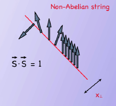
Figure 3: Orientational moduli on the string world sheet are depicted by arrows.

3.1 The simplest model

In the simplest scenario axions (a massless or nearly massless field defined on the circle) is the only modulus on the string (except the translational moduli, of course). The simplest model of this type is obtained from Witten’s superconducting string model wit1 by its reduction. Namely, we will downgrade one of two U(1)’s of the Witten model to a global symmetry, rather than local,

$${\mathcal{L}} = -\frac{1}{4g^{2}}\,F_{\mu\nu}F^{\mu\nu}+|{\mathcal{D}}_{\mu}\phi|^{2}-\frac{\lambda_{\phi}}{4}\,\left(\phi^{2}-v_{\phi}^{2}\right)^{2}$$ (3)

$$+ |\partial_{\mu}\chi|^{2}-\frac{\lambda_{\chi}}{4}\,\left(\chi^{2}-v_{\chi}^{2}\right)^{2}-\beta\phi^{2}\,\chi^{2}\,.$$

This model is a crossbreed between those used in Sh1 ; Sh2 . If the constants $\lambda_{\phi,\chi}$ and $\beta$ are appropriately chosen, the field $\phi$ condenses in the vacuum, Higgsing the gauge U(1) symmetry and, simultaneously, stabilizing the field $\chi$. Then in the vacuum $\langle\chi\rangle_{\rm vac}=0$ which implies that the global U(1) associated with the $\chi$ phase rotations remains unbroken. The theory (3) obviously supports a string which is almost the Abrikosov string. There is an important distinction, however. In the string core $\phi=0$, and the $\beta\phi^{2}\,\chi^{2}$ term stabilizing $\chi$ is switched off. Having $\chi=0$ inside the string is energetically inexpedient. Thus the string solution has $\chi\neq 0$ in the core wit1 . This spontaneously breaks the global U(1) on any given string solution. As a result, a massless phase field $\in{\rm U}(1)$ – an axion – is localized on the string. The world-sheet theory becomes

$$S=\int dt\,dz\,\left\{T\left[(\partial_{\mu}x_{0})^{2}+(\partial_{\mu}y_{0})^{2}\right]+f^{2}(\partial_{\mu}\alpha)^{2}\right\}$$ (4)

where $T$ is the string tension, $f$ is a (dimensionless) axion constant which can be expressed in terms of the bulk parameters, $t$ is time, $z$ is the coordinate along the string while $x_{0}$ and $y_{0}$ are perpendicular coordinates. They can be combined as $x_{\perp}=\{x_{1},\,x_{2}\}$, where $x_{\perp}$ depends on $t$ and $z$,

$$x_{\perp}=x_{\perp}(t,z)\,.$$

Moreover, $\alpha(t,z)$ is the phase field on the world sheet, $\alpha\leftrightarrow\alpha\pm 2\pi\leftrightarrow\alpha\pm 4\pi\,...\,$. In other words, the target space of $\alpha$ is the unit circle.

Now, let us take a long Abrikosov string and and bend it into a circle of circumference $L$, see Fig 4 (I assume $L\gg\ell$ where $\ell$ is the string thickness).

Figure 4: A torus made of the bent Abrikosov flux tube. The dashed line along the large period of the torus is the line of constant $\alpha$ (say, $\alpha=0$).

If $\alpha$ is constant along $z$ (say, $\alpha=0$), this configuration is obviously unstable. Minimizing its energy, the torus will shrink until $L$ becomes of the order of $\ell$, and then the string will annihilate. However, one can stabilize it by forcing $\alpha$ to wind along $z$ in such a way as to make the full $2\pi$ winding when $z$ changes from 0 to $L$,

$$\alpha(t,z)=2\pi z/L\,.$$ (5)

Note that $\alpha$ linearly depending on $z$ goes through the equation of motion on the world sheet, $\partial^{2}\alpha=0$. It is not difficult to estimate the value of $L$. Indeed, the string energy is

$$E=TL+\frac{(2\pi\,f)^{2}}{L}$$ (6)

Minimizing (6) with respect to $L$ we get

$$L=2\pi f/\sqrt{T}\,.$$ (7)

Making $f$ large enough we can always force $L$ to be much larger than the flux tube thickness $\ell$ which is roughly speaking of the order of $1/\sqrt{T}$. Note that for $k$ windings $L=2\pi f\,k/\sqrt{T}\,$.

The soliton of the type discussed above was first constructed in Sh1 where it goes under a special name “vorton” (in the context of cosmic strings; for a recent review and a rather extended list of references see radu ). Its classical stability is due to a nontrivial Hopf topological number Fadd . In the limit $L\gg\ell$ the Hopf soliton is also stable with regards to the quantum tunneling annihilation.

A similar Hopf soliton, albeit with a richer internal structure, was obtained in BMS in the framework of ${\mathcal{N}}=2\,$supersymmetric QED, see Fig. 5.

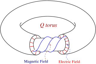
Figure 5: Twisted torus constructed in BMS . This Hopf soliton is also topologically stable.

3.2 Axion-induced deconfinement of kinks in two dimensions

Now I will pass to the axion impact Gorsky on “genuinely” non-Abelian strings, with the orientational moduli on the world sheet described by the CP$(N-1)$ model. In the gauged formulation the CP$(N-1)$ model can be written as

$${\cal L}=\frac{2}{g^{2}}\,\left[\left(\partial_{\alpha}+iA_{\alpha}\right)n^{*}_{\ell}\left(\partial_{\alpha}-iA_{\alpha}\right)n^{\ell}-\lambda\left(n^{*}_{\ell}n^{\ell}-1\right)\right]\,,$$ (8)

where $n^{\ell}$ is an $N$-component complex filed, $\ell=1,2,...,N$, subject to the constraint

$$n_{\ell}^{*}\,n^{\ell}=1\,.$$ (9)

This constraint is implemented by the Lagrange multiplier $\lambda$ in Eq. (8). The field $A_{\alpha}$ in this Lagrangian is also auxiliary, it enters with no derivatives and can be eliminated by virtue of the equations of motion,

$$A_{\alpha}=-\frac{i}{2}\,n^{*}_{\ell}\stackrel{{\scriptstyle\leftrightarrow}}{{\partial_{\alpha}}}n^{\ell}\,.$$ (10)

Substituting Eq. (10) in the Lagrangian, we rewrite it in the form

$${\cal L}=\frac{2}{g^{2}}\,\left[\partial_{\alpha}n^{*}_{\ell}\,\partial_{\alpha}n^{\ell}+(n_{\ell}^{*}\partial_{\alpha}n^{\ell})^{2}-\lambda\left(n^{*}_{\ell}n^{\ell}-1\right)\right]\,.$$ (11)

The coupling constant $g^{2}$ is asymptotically free, and defines a dynamical scale $\Lambda$ of the theory by virtue of the dimensional transmutation,

$$\Lambda^{2}=M_{\rm uv}^{2}\exp\left(-\frac{8\pi}{Ng^{2}_{0}}\right)\,,$$ (12)

where $M_{\rm uv}$ is the ultraviolet cut-off and $g^{2}_{0}$ is the bare coupling.

At first, let us forget for a while about the axion and outline the solution of the “axionless” CP$(N-1)$ model (8) at large $N$ W79 . To the leading order it is determined by one loop and can be summarized as follows: the constraint (9) is dynamically eliminated so that all $N$ fields $n^{\ell}$ become independent degrees of freedom with the mass term $\Lambda$. The photon field $A_{\mu}$ acquires a kinetic term

$${\cal L}_{\gamma\,\,\rm kin}=-\frac{1}{4e^{2}}F_{\mu\nu}^{2}\,,\qquad e^{2}=\frac{12\pi\Lambda^{2}}{N}\,,$$ (13)

and also becomes “dynamical.” The quotation marks here are used because in two dimensions the kinetic term (13) does not propagate any physical degrees of freedom; its effect reduces to an instantaneous Coulomb interaction. This is best seen in the $A_{1}=0$ gauge. In this gauge the above kinetic term takes the form $(\partial_{z}A_{0})^{2}$ while the interaction is

$$A_{\alpha}J^{\alpha}=A_{0}J^{0}\,,\qquad J^{\alpha}=n^{*}_{\ell}\stackrel{{\scriptstyle\leftrightarrow}}{{\partial_{\alpha}}}n^{\ell}\,.$$ (14)

Since $A_{0}$ enters in the Lagrangian without time derivative, it can be eliminated by virtue of the equation of motion leading to the instantaneous Coulomb interaction

$$J_{0}\,\partial_{z}^{-2}\,J_{0}\,.$$ (15)

In two dimensions the Coulomb interaction is proportional to $|z|\,,$ implying linear confinement acting between the $n,\,\,\bar{n}$ “quarks” W79 . Only $n\,\bar{n}$ pairs are free to move along the string.

The axion part of the Lagrangian can be written as follows:

$${\cal L}_{a}=f_{a}^{2}\,(\partial_{\mu}a)^{2}+\frac{a}{2\pi}\,\varepsilon_{\alpha\gamma}\partial^{\alpha}A^{\gamma}\,,$$ (16)

where $A^{\gamma}$ is defined in Eq. (10), and $f_{a}$ is a (dimensionless) axion constant. I will continue to assume that $f_{a}\gg 1$.

Bringing kinetic terms to canonical normalization one obtains

$$-\frac{1}{4}F^{2}_{\mu\nu}+\frac{e}{2\pi f_{a}}\,a\,\varepsilon_{\alpha\gamma}\partial^{\alpha}A^{\gamma}+(\partial_{\mu}a)^{2}+e\,A_{\alpha}J^{\alpha}\,.$$ (17)

The expression for $e^{2}$ is given in (13). The axion field represents a single degree of freedom. The role of the “photon” is that upon diagonalization we get a massive spin-zero particle, with mass of the order of $f_{a}^{-1}\Lambda N^{-1/2}$. Indeed, taking account of the photon-axion mixing amounts to summing the infinite series of tree graphs,

$$e^{2}J^{0}J^{0}\left\{\frac{1}{p^{2}}+\frac{1}{p^{2}}\left(\frac{e}{2\pi f_{a}}\right)^{2}\,\frac{1}{p_{\mu}^{2}}+...\right\}=-e^{2}J_{\alpha}J^{\alpha}\,\,\frac{1}{p_{\mu}^{2}-\left(\frac{e}{2\pi f_{a}}\right)^{2}}\,,$$ (18)

where $p$ is the spatial component of the momentum transfer $p_{\mu}$, and I used Eqs. (15) and (17), and the current conservation. The “ex-photon” mass is determined by the position of the pole in (18).

As a result, the long distance force responsible for confinement disappears, giving place to deconfinement at distances $\gg m_{a}^{-1}$.

The axion-induced liberation of the $n$ fields at distances $\gg m_{a}^{-1}$ demonstrated above is a two-dimensional counterpart of domain-wall deconfinement in four-dimensions Gab2000 ; GabS . The parallel becomes even more pronounced in the (string-inspired) formalism which ascends to susskind (in connection with walls it was developed in Gab2000 and discussed in dvali in another context). In this formalism one introduces an (auxiliary) antisymmetric three-form gauge field $C_{\alpha\beta\gamma}$, while the four-dimensional axion is replaced by an antisymmetric two-form field $B_{\mu\nu}$ (the Kalb–Ramond field). In four dimensions the gauge three-form field has no propagating degrees of freedom while the Kalb–Ramond field $B_{\mu\nu}$ presents a single degree of freedom. The domain walls are the sources for $C_{\alpha\beta\gamma}$, much in the same way as the kinks are the sources for $A_{0}$ in two dimensions. The field strength four-form built from $C_{\alpha\beta\gamma}$ is constant (cf. $F_{01}$ in two dimensions). The $C_{\alpha\beta\gamma}B_{\mu\nu}$ mixing produces one massive physical degree of freedom, a four-dimensional massive axion. Simultaneously, the domain-wall confinement is eliminated at distances $\gg m_{a}^{-1}$. Everything is parallel to the two-dimensional CP$(N-1)$ world-sheet theory.

4 Four-dimensional axion and non-Abelian strings

Now, I address a different problem: a non-Abelian string soliton coupled with a four-dimensional axion existing in the bulk. We introduce a four-dimensional axion in the bulk theory which supports non-Abelian strings; confined monopoles are seen as kinks in the world-sheet theory (CP$(N-1)$). What’s the impact of this four-dimensional axion on dynamics of strings/confined monopoles?

4.1 The bulk model with non-Abelian strings

The appropriate bulk theory (nonsupersymmetric) is given in Eq. (1) where $T^{a}$ stands for the generator of the gauge SU(2) group,

$$\nabla_{\mu}\,\Phi\equiv\left(\partial_{\mu}-\frac{i}{\sqrt{2N}}\;A_{\mu}-iA^{a}_{\mu}\,T^{a}\right)\Phi\,,$$ (19)

and $\theta$ is the vacuum angle, to be promoted to the axion field,

$$\theta\to\theta+a\to a(x)\,.$$ (20)

The last term forces $\Phi$ to develop a vacuum expectation value (VEV) while the last but one term forces the VEV to be diagonal,

$$\Phi_{\rm vac}=\sqrt{\xi}\,{\rm diag}\,\{1,1\}\,.$$ (21)

This VEV results in the spontaneous breaking of both gauge and flavor SU(2)’s. A diagonal global SU(2) survives, however, namely

$${\rm U(2)}_{\rm gauge}\times{\rm SU(2)}_{\rm flavor}\to{\rm SU(2)}_{\rm diag}\,.$$ (22)

The vacuum is color-flavor locked.

One can combine the $Z_{2}$ center of SU($2$) to get a topologically stable string solution HT1 ; ABEKY possessing both windings, in SU($2$) and U(1) since $\pi_{1}\left({\rm SU}(N)\times{\rm U}(1)/Z_{N}\right)\neq 0\,.$ Their tension is $1/2$ of that of the Abrikosov string. It is rather obvious that these strings have orientational zero modes associated with rotation of their color flux inside the non-Abelian subgroup SU($2$) of the gauge group Trev . This implies that the effective low-energy theory on the string world sheet includes both the standard Nambu–Goto action associated with translational moduli and a sigma model part which describes internal dynamics of the orientational moduli, CP$(N-1)$. The four-dimensional axion interaction is added in (8) through the term

$$-\frac{\theta+a}{2\pi}\,\,\varepsilon^{nk}\,\partial_{n}\,n^{*}\partial_{k}\,n\,,$$ (23)

where $\theta$ coincides with the four-dimensional $\theta$ while $a(t,\vec{x})$ is the four-dimensional pseudoscalar field propagating in the bulk.

4.2 Monopole-antimonopole “mesons” vs. axion clouds

What happens with the monopole-antimonopole meson on the non-Abelian string in the presence of the four-dimensional axion? Given the discussion above one might suspect that the four-dimensional axion induces deconfinement of monopoles localized on the non-Abelian string, much in the same way as the two-dimensional axion. Now I will argue that this does not happen.

The classical action of the four dimensional bulk axion field is

$$L_{a}=\int d^{4}x\left[f_{a}^{2}(\partial a)^{2}+\frac{ia}{32\pi^{2}}F^{a}_{\mu\nu}\tilde{F}^{a}_{\mu\nu}\right]\,,$$ (24)

where in the case at hand $f_{a}$ has dimension of mass. The axion has a small mass generated by four-dimensional bulk instantons

$$m_{a}^{2}\sim\frac{\Lambda^{4}_{4}}{f_{a}^{2}}\,\left(\frac{\Lambda_{4}}{\sqrt{\xi}}\right)^{b-4}\,,\qquad f_{a}\gg\Lambda_{4}\,,$$ (25)

where $b$ is the first coefficient of the $\beta$ function in the theory (1), but this mass plays no role in what follows.

The impact of the bulk axion on the non-Abelian string is two-fold. First, the axion gets coupled to the translational moduli of the string. Assuming that the string collective coordinates adiabatically depend on the world-sheet coordinates we get for this coupling

$${\cal L}_{a}^{(1)}\sim\xi\int d^{4}x\,a(x)\,\varepsilon^{ij}\,\varepsilon_{\alpha\beta}\,\partial_{i}x^{\alpha}_{\perp}\,\partial_{j}x^{\beta}_{\perp}\,\,\delta^{(2)}(x-x_{\rm string}(t,z)),$$ (26)

where the indices $i,j=0,3$ run over the string world sheet coordinates while the indices $\alpha,\beta=1,2$ are orthogonal to the string world-sheet. (One could rewrite this expression in a covariant form trading the axion field for the Kalb–Ramon two-index field $B_{\mu\nu}(x)$ but this is not necessary.) The coupling (26) is not specific for non-Abelian strings, it is generated in the case of the Abrikosov strings as well.

Now, let us discus orientational moduli. It is easy to see that no mixed $n$-$x_{\perp}$ terms appear in the axion Lagrangian (at least, in the the quadratic order in derivatives). The bulk axion generates a quadratic in $n$ coupling, as is clearly seen from Eq. (23). The impact of this term in the axion Lagrangian can be summarized as follows:

$${\cal L}_{a}^{(2)}\sim\int d^{4}x\,a(x)\,\varepsilon^{nk}\,\,\partial_{n}\,n^{*}\partial_{k}\,n\,\,\delta^{(2)}(x-x_{\rm string}(t,z)),$$ (27)

For a short while forget about axions and consider the monopole-antimonopole pair attached to the string. The energy of this monopole-antimonopole meson is of order of $(\Lambda^{2}/N)\,L,$ where $L$ is the distance between the monopole and antimonopole along the string. What happens upon switching on the four-dimensional axion field?

Logically speaking, the axion field could develop a nonvanishing expectation value $a=2\pi$ on the string between the monopole and antimonopole positions, equalizing the string energies inside and outside the pair, and screening the confinement force. This is exactly what happened with the two-dimensional axion. To see whether or not a similar effect occurs with four-dimensional axions we have to examine a field configuration in which $\langle a\rangle=0$ everywhere in the bulk except a region adjacent to the monopole-antimonopole separation interval, as depicted in Fig. 6.

Figure 6: The monopole-antimonopole meson together with the axion cloud. The region of the string between the monopole and antimonopole is not exited because the value of the axion field is nonvanishing inside the axion cloud, $a=2\pi$.

We have to check the energy balance assuming there is an axion cloud such that on the string inside the monopole-antimonopole separation interval $\langle a\rangle=2\pi$, which would let (anti)monopoles move freely along the string, with no confinement along the string.

It is not difficult to estimate the energy of the axion cloud. The transverse size of the cloud (in two directions perpendicular to the string) must be of order of $m_{a}^{-1}$. The longitudinal dimension is $L$, see Fig. 6. Assuming that $L\gg m_{a}^{-1}$ we get

$$E_{\rm cloud}\sim f_{a}^{2}\,L,$$ (28)

to be compared to the energy $(\Lambda^{2}/N)\,L$ of the monopole-antimonopole meson. Since $f_{a}$ is supposed to be very large compared to $\Lambda$ we see that the energy of the axion cloud (28) is much larger than the monopole-antimonopole meson energy. Developing a compensating axion cloud is energetically disfavored. Therefore we conclude that there is no monopole deconfinement driven by four-dimensional axions.

4.3 Cosmic non-Abelian string and axion emission

Hashimoto and Tong suggested Hashimoto to consider non-Abelian strings as cosmic string candidates. It is worth discussing possible signatures of such non-Abelian strings in the context of axion physics. Obviously, both, translational and orientational modes can be excited in collisions. In the latter case one can think of production of energetic monopole-antimonopole pairs attached to the string and bound in mesons by the confining potential along the string, as I described above. On the part of the string between the monopole and antimonopole (the kink and antikink) the state of the string is described by a quasivacuum with $k=-1$. In this state

$$\langle\varepsilon^{nk}\,\,\partial_{n}\,n^{*}\partial_{k}\,n\rangle\sim\Lambda^{2}/N\,.$$ (29)

The topological charge density is localized in the domain of the excited part of the string, and is approximately constant in this domain. Therefore, as is clear from Eq. (27), this interval, whose length $L$ oscillates in accordance with the monopole-antimonopole motion, will serve as a source term in the equation for the axion field. Assume that the energy of the kink-antikink pair $E\gg\Lambda$ so that they can be treated quasiclassically. The distance $L$ between the kink and antikink will oscillate between $-L_{0}$ and $L_{0}$ where $L_{0}\sim E/\Lambda^{2}$ with the frequency $\omega\sim\Lambda^{2}/E$,

$$L(t)=L_{0}\,e^{i\omega t}\,.$$ (30)

Therefore, for a distant observer the monopole-antimonopole meson is seen as a point-like source with the interaction term

$${\Lambda^{2}}\,\int d^{4}x\,a(x)\,L(t)\,\delta^{3}(r-r_{0}),$$ (31)

where $r_{0}$ is a position of the meson on the string. The intensity of the axion radiation from this point-like source can be estimated as

$$I_{a}\sim\omega^{2}\,\frac{\Lambda^{4}L^{2}_{0}}{f_{a}^{2}}\,\frac{1}{r^{2}}\sim\omega^{2}\,\frac{E^{2}}{f_{a}^{2}}\,\frac{1}{r^{2}}\,,$$ (32)

where $r$ is the distance to the observer.

Of course the string produces axion radiation also due to coupling with translational modes, Eq. (26). This radiation is seen as coming from a linear source, and can be estimated (per unit length) as

$$I_{a}\sim\frac{\xi^{1/2}}{f_{a}^{2}}\,\frac{E^{2}}{\ell^{2}}\,\frac{1}{\rho}\,.$$ (33)

Here $\rho$ is the distance from the string to the observer in the plane orthogonal to the string, $E$ is the total excitation energy and $\ell$ is the length of the excited part of the string. This radiation is not specific for non-Abelian strings. Abelian strings produce this radiation as well.

We see that the non-Abelian string is seen by a distant observer as a linear source of the axion radiation (33), with additional point-like sources of the axion radiation (32) located on the linear source at the positions of the monopole-antimonopole mesons. The rate of the axion radiation depends of $f_{a}$. The oscillating kink-antikink pair will shake off energy until exhaustion. The time duration of the monopole-antimonopole meson de-excitation can be estimated as $T\sim E^{2}f_{a}^{2}$.

5 Conclusions

The existence of axion-like particles is almost unavoidable in the framework of string theory. The impact of axions on various field-theoretic strings (flux tubes) is multifaceted. Two-dimensional axions can stabilize toric Hopf solitons, liberate kinks, confined in the absence of axion, and do other equally remarkable jobs. Introducing a bulk axion in the “benchmark” nonsupersymmetric model Gorsky2 supporting non-Abelian strings we observe that the four-dimensional axion does not lead to monopole deconfinement. In the context of cosmic strings, the axion emission due to excitations of non-Abelian strings occurs in a different way compared to that from Abelian string. Energetic pairs of confined and oscillating (anti)monopoles act as an additional pointlike source specific to non-Abelian strings.

In coclusion, I would like to mention that a new study of toric Hopf solitons stabilized by axion-like fields is under way now GSYnew .

References

- (1) S. Weinberg, Phys. Rev. Lett. 40, 223 (1978).
- (2) F. Wilczek, Phys. Rev. Lett. 40, 279 (1978).
- (3) J. E. Kim, Phys. Rev. Lett. 43, 103 (1979).
- (4) M. A. Shifman, A. I. Vainshtein and V. I. Zakharov, Nucl. Phys. B 166, 493 (1980).
- (5) A. R. Zhitnitsky, Sov. J. Nucl. Phys. 31, 260 (1980) [Yad. Fiz. 31, 497 (1980)].
- (6) M. Dine, W. Fischler and M. Srednicki, Phys. Lett. B 104, 199 (1981).
- (7) G. Gabadadze and M. Shifman, Int. J. Mod. Phys. A 17, 3689 (2002) [arXiv:hep-ph/0206123].
- (8) A. Hanany and D. Tong, JHEP 0307, 037 (2003) [hep-th/0306150].
- (9) R. Auzzi, S. Bolognesi, J. Evslin, K. Konishi and A. Yung, Nucl. Phys. B 673, 187 (2003) [hep-th/0307287].
- (10) M. Shifman and A. Yung, Phys. Rev. D 70, 045004 (2004) [hep-th/0403149].
- (11) A. Hanany and D. Tong, JHEP 0404, 066 (2004) [hep-th/0403158].
- (12) M. Shifman and A. Yung, Supersymmetric Solitons, (Cambridge University Press, 2009).
- (13) K. Hashimoto and D. Tong, JCAP 0509, 004 (2005) [arXiv:hep-th/0506022].
- (14) A. Gorsky, M. Shifman and A. Yung, Phys. Rev. D 73, 125011 (2006) [arXiv:hep-th/0601131].
- (15) A. Abrikosov, Sov. Phys. JETP 32 1442 (1957) [Reprinted in Solitons and Particles, Eds. C. Rebbi and G. Soliani (World Scientific, Singapore, 1984), p. 356].
- (16) H. Nielsen and P. Olesen, Nucl. Phys. B61 45 (1973) [Reprinted in Solitons and Particles, Eds. C. Rebbi and G. Soliani (World Scientific, Singapore, 1984), p. 365].
- (17) A. Gorsky, M. Shifman and A. Yung, Phys. Rev. D 71, 045010 (2005) [arXiv:hep-th/0412082].
- (18) E. Witten, Nucl. Phys. B 249, 557 (1985).
- (19) R. L. Davis and E. P. S. Shellard, Phys. Lett. B 207, 404 (1988); Phys. Lett. B 209, 485 (1988).
- (20) Y. Lemperiere and E. P. S. Shellard, Phys. Rev. Lett. 91, 141601 (2003) [arXiv:hep-ph/0305156].
- (21) E. Radu and M. S. Volkov, Phys. Rept. 468, 101 (2008) [arXiv:0804.1357 [hep-th]].
- (22) L. D. Faddeev and A. J. Niemi, Nature 387, 58 (1997) [hep-th/9610193]; Phys. Rev. Lett. 82, 1624 (1999) [hep-th/9807069].
- (23) S. Bolognesi and M. Shifman, Phys. Rev. D 76, 125024 (2007) [arXiv:0705.0379 [hep-th]].
- (24) E. Witten, Nucl. Phys. B 149, 285 (1979).
- (25) G. Gabadadze and M. A. Shifman, Phys. Rev. D 62, 114003 (2000) [hep-ph/0007345].
- (26) R. Kallosh, A. D. Linde, D. A. Linde and L. Susskind, Phys. Rev. D 52, 912 (1995) [hep-th/9502069].
- (27) G. Dvali, Three-Form Gauging of Axion Symmetries and Gravity, hep-th/0507215, unpublished.
- (28) A. Gorsky, M. Shifman and A. Yung, work in progress.