Escape of stars from gravitational clusters in the Chandrasekhar model

Abstract

We study the evaporation of stars from globular clusters using the simplified Chandrasekhar model [S. Chandrasekhar, Astrophys. J. 97, 263 (1943)]. This is an analytically tractable model giving reasonable agreement with more sophisticated models that require complicated numerical integrations. In the Chandrasekhar model: (i) the stellar system is assumed to be infinite and homogeneous (ii) the evolution of the velocity distribution of stars $f(v,t)$ is governed by a Fokker-Planck equation, the so-called Kramers-Chandrasekhar equation (iii) the velocities $|v|$ that are above a threshold value $R>0$ (escape velocity) are not counted in the statistical distribution of the system. In fact, high velocity stars leave the system, due to free evaporation or to the attraction of a neighboring galaxy (tidal effects). Accordingly, the total mass and energy of the system decrease in time. If the star dynamics is described by the Kramers-Chandrasekhar equation, the mass decreases to zero exponentially rapidly. Our goal is to obtain non-perturbative analytical results that complement the seminal studies of Chandrasekhar, Michie and King valid for large times $t\rightarrow+\infty$ and large escape velocities $R\rightarrow+\infty$. In particular, we obtain an exact semi-explicit solution of the Kramers-Chandrasekhar equation with the absorbing boundary condition $f(R,t)=0$. We use it to obtain an explicit expression of the mass loss at any time $t$ when $R\rightarrow+\infty$. We also derive an exact integral equation giving the exponential evaporation rate $\lambda(R)$, and the corresponding eigenfunction $f_{\lambda}(v)$, when $t\rightarrow+\infty$ for any sufficiently large value of the escape velocity $R$. For $R\rightarrow+\infty$, we obtain an explicit expression of the evaporation rate that refines the Chandrasekhar results. More generally, our results can have applications in other contexts where the Kramers equation applies, like the classical diffusion of particles over a barrier of potential (Kramers problem).

1 Introduction

In a seminal paper, Chandrasekhar [1] developed a Brownian theory of stellar dynamics in order to determine the rate of escape of stars from globular clusters. Small groups of stars tend to approach a statistical equilibrium state (described by the Boltzmann distribution) as a result of stellar encounters. However, high energy stars are not bound to the system and escape to infinity. For an isolated system, the average escape velocity for all stars in the cluster is fixed by the virial theorem according to the equation $R=2v_{rms}$ where $v_{rms}=\langle v^{2}\rangle^{1/2}$ is the root-mean-square velocity (RMS) [2]. If the system, e.g. a globular cluster, is submitted to tidal forces from a neighboring galaxy, the escape velocity can be smaller. Therefore, stars clusters tend to slowly evaporate. This evaporation was first studied by Ambartsumian [3] and Spitzer [4] using phenomenological arguments. They estimated the evaporation time by removing a fraction $\gamma=7.38\ 10^{-3}$ of stars every relaxation time, where $\gamma$ is the fraction of particles in a Maxwellian distribution that have speeds exceeding twice the RMS velocity. In a more precise treatment, Chandrasekhar [1] described the “collisional” evolution of a stellar system by a Fokker-Planck equation (the nowadays called Kramers equation) involving a diffusion term in velocity space modeling the erratic motion of the stars and a friction term that appears to be necessary to drive the system towards the Boltzmann distribution predicted by statistical mechanics (fluctuation-dissipation theorem). The diffusion coefficient and the “dynamical friction”, satisfying the Einstein relation, were independently justified from kinetic theory by explicitly calculating the first and second moments of the velocity increment suffered by a star during a succession of binary encounters. In order to account for evaporation, Chandrasekhar imposed as a boundary condition that the distribution function $f(v,t)$ vanishes when the star velocity reaches a maximum value $|v|=R$. He then reduced the problem to the study of an eigenvalue equation in a bounded domain of velocities $|v|\leq R$. The fundamental eigenvalue gives the exponential evaporation rate of the stars from the cluster for $t\rightarrow+\infty$ and the associated eigenfunction gives the quasi-stationary distribution function of the system. This distribution function is close to the Boltzmann distribution for low velocities and tends to zero at the escape velocity. Chandrasekhar solved the eigenvalue problem by transforming the Kramers equation into a Schrödinger equation (with imaginary time) for a quantum oscillator in a box and by expanding the solutions of that equation in the form of a series. He obtained (semi-explicit) analytical results in the $R\rightarrow+\infty$ limit or, equivalently, for a small evaporation rate $\lambda(R)\rightarrow 0$. In his first treatment [1], he assumed that the diffusion coefficient is constant and in a more exact theory [5], he took into account the dependence of the diffusion coefficient with the velocity. His work was followed by Spitzer & Härm [6] who determined the escape rate (eigenvalue) and the quasi-stationary distribution function (eigenfunction) numerically for any value of the escape velocity $R$. Then, Michie [7] and King [8] obtained for $R\rightarrow+\infty$ a simple analytical expression of the quasi-stationary distribution function in the form of a lowered isothermal distribution which vanishes at the escape velocity. This leads to the so-called Michie-King model [2] that is asymptotically valid in the limit $R\rightarrow+\infty$.

The Chandrasekhar model described previously is based on simplifying assumptions. It is first assumed that the system is spatially homogeneous and infinite while globular clusters are highly inhomogeneous and limited in space. On the other hand, the collisional evolution of the system is modeled by the Kramers equation while a more relevant equation is the gravitational Landau equation that is the standard kinetic equation of stellar dynamics [2, 9, 10, 11]. The Kramers equation corresponds to a canonical description in which the system is assumed to be in contact with a thermal bath from which it can extract energy so that the temperature $T$ is fixed. Alternatively, the Landau equation corresponds to a microcanonical description in which the system is assumed to be isolated so that the energy $E$ is conserved. Since globular clusters are isolated Hamiltonian systems (up to the slow evaporation process), the microcanonical description appears to be more relevant. Therefore, when we take into account spatial inhomogeneity and model the encounters in a self-consistent way, the proper model to consider is formed by the gravitational Landau equation coupled to the Poisson equation. In order to go beyond the limitations of the Chandrasekhar model and obtain more accurate rates of escape, the astrophysicists have performed numerical simulations of stellar systems. Different types of simulations have been performed. They solved (i) the $N$-body Hamiltonian problem associated to the Newton equations [12] (ii) the hydrodynamic moments of the Landau equation [13, 14] (iii) the $N$-body problem where the effect of encounters is modeled by Monte Carlo methods [15, 16, 17], and (iv) the orbit-averaged-Fokker-Planck equation [18]. These methods are reviewed in the books of Spitzer [9] and Binney & Tremaine [2] and in the reviews [19, 20]. In these numerical works, the spatial inhomogeneity of the cluster is properly taken into account.

These simulations have led to the following scenario for the evolution of globular clusters [2, 9]. In a first regime, a self-gravitating system initially out-of-mechanical equilibrium undergoes a process of violent collisionless relaxation towards a virialized state. In this regime, the dynamical evolution of the cluster is described by the Vlasov-Poisson system and the phenomenology of violent relaxation has been described by Hénon [21], King [22] and Lynden-Bell [23]. Numerical simulations that start from cold and clumpy initial conditions generate a quasi stationary state (QSS) that fits the de Vaucouleurs $R^{1/4}$ law quite well [24]. The inner core is almost isothermal (as predicted by Lynden-Bell [23]) while the velocity distribution in the envelope is radially anisotropic and the density profile decreases like $r^{-4}$ [25, 26]. One success of Lynden-Bell’s statistical theory of violent relaxation is to explain the isothermal core without recourse to “collisions”. By contrast, the structure of the halo cannot be explained by Lynden-Bell’s theory as it is a result of an incomplete relaxation. On longer timescales, encounters between stars must be taken into account and the dynamical evolution of the cluster is governed by the Vlasov-Landau-Poisson system which is the standard model of stellar dynamics. This collisional regime is appropriate to understand the actual structure of globular clusters. In this regime, the system passes through a succession of quasi stationary states (QSS) that are steady states of the Vlasov equation slowly evolving in time due to the cumulative effect of encounters. The first stage of the collisional evolution is driven by evaporation. Due to a series of weak encounters, the energy of a star can gradually increase until it reaches the local escape energy; in that case, the star leaves the system. Numerical simulations [9] show that during this regime the system reaches a quasi-stationary state that slowly evolves in amplitude due to evaporation as the system loses mass and energy. This quasi stationary distribution function (DF) is close to the Michie-King model. The system has a core-halo structure. The core is isothermal while the stars in the outer halo move in predominantly radial orbits. Therefore, the distribution function in the halo is anisotropic. The density follows the isothermal law $\rho\sim r^{-2}$ in the central region (with a core of almost uniform density) and decreases like $\rho\sim r^{-7/2}$ in the halo [2]. Due to evaporation, the halo expands while the core shrinks as required by energy conservation. At some point of the evolution, when the energy passes below a critical value (or when the density contrast becomes sufficiently high), the system undergoes an instability related to the Antonov [28] instability and the gravothermal catastrophe takes place [29]. This instability is due to the negative specific heat of the inner system that evolves by losing energy and thereby growing hotter (see reviews in [10, 30]). This leads to core collapse [2]. Mathematically speaking, core collapse would generate a finite time singularity: if the evolution is modeled by the orbit-averaged-Fokker-Planck equation, Cohn [18] finds that the collapse is self-similar, that the central density becomes infinite in a finite time and that the density behaves like $\rho\sim r^{-2.23}$ (if the evolution is modeled by the Landau-Poisson system, it is argued in [31] that the density behaves like $\rho\propto r^{-3}$ in the final stage of the collapse). In reality, if we come back to the $N$-body system, core collapse is arrested by the formation of binary stars. These binaries can release sufficient energy to stop the collapse [32] and even drive a re-expansion of the cluster in a post-collapse regime [33]. Then, in principle, a series of gravothermal oscillations should follow [34]. In practice, the processes of evaporation and core collapse take place simultaneously so that it is difficult to isolate the effect of any single process in the evolution of a globular cluster.

Concerning the evaporation process, the Princeton code was the first code to yield reliable evaporation rates [35] giving $t_{evap}=-N(dN/dt)^{-1}\simeq 300t_{rh}$ for isolated clusters. These results are not very different from those obtained with the spatially homogeneous Kramers-Chandrasekhar equation. Our goal in this paper is not to make a realistic modeling of stellar systems but rather to consider simple models of evaporation that are analytically tractable. Therefore, we shall use the Chandrasekhar model which yields a reasonable description of the evaporation process in globular clusters and which can be studied analytically. Chandrasekhar solved the problem perturbatively: he first considered the long time limit $t\rightarrow+\infty$ so that the distribution function $f_{R}(v,t)$ is dominated by the contribution of the fundamental eigenmode $f_{R}(v)e^{-|\lambda(R)|t}$ and then took the limit $R\rightarrow+\infty$ to obtain an approximate expression of the quasi-stationary distribution $f_{R}(v)$ (fundamental eigenfunction) and escape rate $\lambda(R)$ (fundamental eigenvalue). In this paper, we shall reconsider the Chandrasekhar problem on a new angle which allows to obtain non-perturbative results. In particular, we find an exact semi-explicit solution of the Kramers equation with boundary condition $f(v,t)=0$ when $|v|=R$. This solution $f(v,t)$ depends on the remaining mass in the cluster $M_{0}(t)$ which satisfies an autonomous equation. We use this general formula to obtain: (i) the mass $M_{0}(t)$ for any fixed time $t$ in the limit $R\rightarrow+\infty$, (ii) an exact integral equation for the eigenvalue $\lambda(R)$ of the fundamental mode (evaporation rate) valid for any sufficiently large $R$, (iii) an exact explicit expression of the fundamental eigenfunction valid for any sufficiently large $R$, and (iv) an explicit asymptotic expression of the evaporation rate when $R\rightarrow+\infty$. Therefore, our approach complements Chandrasekhar’s original work and offers new perspectives. Our main results are, however, restricted to the Kramers equation, i.e. a Fokker-Planck equation with constant diffusion coefficient and quadratic potential (linear friction). A different approach that goes beyond these limitations (but which is restricted to the asymptotic limits $t\rightarrow+\infty$ and $R\rightarrow+\infty$) is developed in Appendix D.

Let us finally note that our approach is not limited to the astrophysical problem mentioned above but that it can have applications in different area. First of all, Chandrasekhar’s study of the rate of escape of stars from globular clusters is closely connected to the classical Kramers [37] problem for the escape rate of a Brownian particle across a potential barrier that has many applications in physics and chemistry (surprisingly, Chandrasekhar [1] did not mention this connection). In that case, the problem is usually formulated in $d=1$ dimension. On the other hand, Chandrasekhar’s procedure has been used in the context of planet formation [38] in order to determine the rate of escape of dust from large-scale vortices (assumed to be present in the solar nebula) due to turbulence. In that case, the problem is two-dimensional. In view of the fundamental nature of the mathematical problem, it seems relevant to develop our formalism in arbitrary dimension of space $d$ in order to cover a wide range of possible applications.

2 Setting of the problem and statement of the results

2.1 Kinetic models on a bounded velocity domain

Basically, the evolution of the distribution function $f(x,v,t)$ of a stellar system is described by the Vlasov-Landau-Poisson equation [2, 9, 10, 11]:

$$\left\{\begin{array}[]{ll}\displaystyle\frac{\partial f}{\partial t}+v\cdot\nabla_{x}f-\nabla\Phi\cdot\nabla_{v}f=\nabla_{v}\cdot\int K(v-v_{*})\left(f(x,v_{*})\nabla_{v}f(x,v)-f(x,v)\nabla_{v}f(x,v_{*})\right)dv_{*},\\ \displaystyle\Delta\Phi=4\pi G\int f\,dv,\\ \displaystyle f(x,v,t=0)=f_{0}(x,v)\geq 0,\ \ (x,v)\in\mathbb{R}^{3}\times\mathbb{R}^{3},\\ \displaystyle\end{array}\right.$$ (2.1)

where $\Phi(x,t)$ is the gravitational potential and $K(u)$ is the following $3\times 3$ matrix

$$K(u)_{ij}=A\frac{|u|^{2}\delta_{ij}-u_{i}u_{j}}{|u|^{3}},$$ (2.2)

where $A=2\pi G^{2}m\ln\Lambda$ is a constant ($G$ is the gravity constant, $m$ the mass of a star and $\ln\Lambda$ the Coulomb logarithm). These equations must be complemented by the boundary condition $f(x,v,t)=0$ if $\epsilon\equiv v^{2}/2+\Phi(x,t)>0$ which expresses the fact that stars with positive energy are lost by the system. Indeed, they are unbound and free to escape to infinity. This is the reason for the evaporation of the star cluster. The Vlasov-Landau-Poisson system (2.1) is the standard model of stellar dynamics. From the Landau equation, the relaxation time due to two-body encounters can be estimated by $t_{R}\sim(N/\ln N)t_{D}$ where $t_{D}$ is the dynamical time and $N$ the number of stars in the system [2]. For large groups of stars like elliptical galaxies ($N\sim 10^{11}$, $t_{D}\sim 10^{8}$ years, age $\sim 10^{8}$ years), the relaxation time is much larger than the age of the universe by several orders of magnitude so that star encounters are completely negligible. In that case, their evolution is described by the Vlasov-Poisson system, i.e. by (2.1) with the r.h.s. taken equal to zero. For smaller groups of stars like globular clusters ($N\sim 10^{5}$, $t_{D}\sim 10^{5}$ years, age $\sim 10^{10}$ years) whose ages are of the same order as the relaxation time, the encounters must be taken into account. The study of the full Vlasov-Landau-Poisson equation is extremely complicated because it involves several processes: (i) violent relaxation in the collisionless regime (ii) gravothermal catastrophe in the collisional regime, and (iii) evaporation. Furthermore, the coupling between the Landau equation and the Poisson equation, and the fact that the distribution function depends on seven variables $(x,v,t)$ in the general case, make these equations untractable without further assumptions. Some simplification can be obtained by averaging over the orbits of the stars thereby obtaining the orbit-averaged-Fokker-Planck equation [2, 9]. For spherical systems, this leads to an equation for the distribution function $f=f(\epsilon,t)$ that depends only on the energy $\epsilon=v^{2}/2+\Phi$ and time $t$. Still, the theoretical study of the orbit-averaged-Fokker-Planck equation remains very complicated. In order to distinguish the contribution of each process occurring in the evolution of a stellar system and to study specifically the evaporation process in a very simple setting (which is our motivation here) we shall make additional simplifying assumptions. First, we shall disregard the spatial structure of the system and assume that the medium under consideration is infinite and homogeneous. If we implement this approximation naively, solving the spatially homogeneous Landau equation for $f(v,t)$, it is found [39] that the r.m.s. velocity decreases due to evaporation while in reality (i.e. when spatial inhomogeneity is retained and the Landau equation is coupled to the Poisson equation) the contraction of the core causes the r.m.s. velocity to increase (as potential energy is converted into kinetic energy faster than the escaping stars carry energy away). This approximation leads therefore to unphysical results. This problem was solved by King [39] by adding artificially in the spatially homogeneous Landau equation an additional outward flux in velocity space. In that case, the decrease in kinetic energy due to evaporation is compensated by the increase in kinetic energy due to contraction. Another solution, that was proposed earlier by Chandrasekhar [1], is to assume that the star under consideration has encounters with a separate group of stars having a fixed (usually assumed Maxwellian) velocity distribution. In that case, the star is able to extract energy from a reservoir imposing its temperature (thermal bath). Therefore, Chandrasekhar models the evolution of the system by a Fokker-Planck equation of the form:

$$\left\{\begin{array}[]{ll}\displaystyle\frac{\partial f}{\partial t}(v,t)=Q_{R}^{FP}(f)(v)=\nabla\cdot\left[D(|v|)\left(\nabla f(v)+\beta f(v)v\right)\right],\ v\in B_{R},\\ \displaystyle f(v,t=0)=f_{0}(v)\geq 0,\ \ v\in B_{R}\\ \displaystyle f(v,t)=0,\ \ \ \mbox{if}\ |v|=R,\end{array}\right.$$ (2.3)

where $D(|v|)$ is some given nonnegative diffusion matrix. The Fokker-Planck equation (2.3) can be derived from the Landau equation (2.1) by making the so-called “thermal bath approximation”, i.e. by replacing the function $f(v_{*})$ in (2.1) by the Maxwell distribution $f(v)={\rho}{(2\pi T)^{-3/2}}{\rm exp}(-{v^{2}}/{2T})$ with inverse temperature $\beta=1/T$ (here, the mass of stars has been included in the temperature). This procedure transforms an integrodifferential (Landau) kinetic equation into a differential (Fokker-Planck) equation and allows an explicit computation of the diffusion coefficient $D(|v|)$ (see [11] and references therein). The Fokker-Planck equation (2.3) can also be derived from a stochastic Langevin equation with a linear friction (Ornstein-Uhlenbeck process) and is called the Kramers equation [37]. Since it was derived independently by Chandrasekhar [1] in the astrophysical context, we will call it here the Kramers-Chandrasekhar equation. Finally, the last condition in (2.3) expresses the fact that a star with velocity above a certain threshold $R$ escapes and is therefore lost by the system. This threshold can be estimated by the following classical argument [2]. The escape speed at $x$ is given by $v_{e}^{2}=-2\Phi(x)$, corresponding to $\epsilon=0$. The mean square escape speed in a system whose density is $\rho(x)$ is therefore $\langle v_{e}^{2}\rangle=\int\rho(x)v_{e}^{2}\,dx/\int\rho(x)\,dx=-(2/M)\int\rho(x)\Phi(x)\,dx=-4W/M$ where $M$ is the total mass and $W$ the potential energy. According to the virial theorem $-W=2K$ where $K=(1/2)M\langle v^{2}\rangle$ is the kinetic energy. Hence $\langle v_{e}^{2}\rangle=4\langle v^{2}\rangle$. For a Maxwellian distribution with temperature $T$, we obtain $R=2\sqrt{3T}$. However this is just an estimate. Furthermore, the escape velocity can be smaller if the system (globular cluster) is subject to the tide of a nearby galaxy. Therefore, for sake of generality, we shall consider $R$ arbitrary. The Fokker-Planck equation (2.3) with proper boundary condition $f(R,t)=0$ was used by Chandrasekhar [1] and others [6, 7, 8] to determine the rate of escape of stars from globular clusters. We shall call it the Chandrasekhar model. This is the model studied in the present paper. For sake of generality, we shall consider these equations in $d$ dimensions.

2.2 Semi-explicit solutions on a bounded velocity domain

In this section, we focus on the Fokker-Planck equation (2.3) with $D\equiv 1$ and boundary condition $f(R,t)=0$. We prove that a semi-explicit solution of this kinetic equation can be given for this model. More precisely, we derive an autonomous relation satisfied by $M_{0}(t)$, the mass remaining in the cluster at time $t$, and then give an explicit expression of the solution $f(v,t)$ in terms of $M_{0}(t)$ and of the initial data $f_{0}(v)$ only. This result will be used to determine the exact (i.e. non perturbative) rate of escape of stars in the Chandrasekhar model (see section 2.3).

Note that the difficulty here comes from the boundedness character of the velocity domain and the presence of the term $vf$ in the drift-diffusion model (2.3), which prevent a direct use of Fourier analysis. Our strategy is to first transform Eq. (2.3) into equivalent equations on the whole domain ${\mathbb{R}}^{d}$ where the boundary condition naturally disappears and is replaced by a source term (see Appendix A). The resulting equation makes sense in the space of distributions and one can use Fourier techniques in this space to work out a semi-explicit solution of the problem.

Proposition 2.1 (Semi-explicit solution of (2.3))

Let $f_{0}$ be a smooth and isotropic initial data supported inside $B_{R}$. The solution to (2.3) when $D\equiv 1$, with initial data $f_{0}$, is given by

$$\begin{array}[]{ll}f(v,t)=&\displaystyle\frac{1}{(2\pi)^{d}}\left(\frac{\pi}{A(0,t)}\right)^{d/2}\int_{B_{R}}f_{0}(v_{*})\ {\rm exp}\left(-\frac{|v-B(0,t)v_{*}|^{2}}{4A(0,t)}\right)dv_{*}\\ &\displaystyle{+}\frac{1}{(2\pi)^{d}}\frac{1}{|{\mathbb{S}}_{1}^{d}|}\int_{0}^{t}ds\left(\frac{\pi}{A(s,t)}\right)^{d/2}M_{0}^{\prime}(s)\int_{\sigma\in{\mathbb{S}}_{1}^{d}}d\sigma\ {\rm exp}\left(-\frac{|B(s,t)R\sigma+v|^{2}}{4A(s,t)}\right),\end{array}$$ (2.4)

where ${\mathbb{S}}_{1}^{d}$ is the unit sphere ${\mathbb{R}}^{d}$ with measure $|{\mathbb{S}}_{1}^{d}|$, $d\sigma$ is the surface element of this unit sphere, and:

$$A(s,t)=\frac{1}{2\beta}\left(1-{\rm exp}(-2\beta(t-s))\right),\ \ \ \ B(s,t)={\rm exp}(-\beta(t-s)).$$

The total mass $M_{0}(t)$ of $f$, defined by

$$M_{0}(t)=\int_{B_{R}}f(v,t)\,dv,$$ (2.5)

is determined from the boundary condition $f(R\omega,t)=0,\ \ \forall\omega\in{\mathbb{S}}_{1}^{d}$ leading to the autonomous equation

$$\begin{array}[]{ll}\displaystyle A(0,t)^{-d/2}&\displaystyle\int_{B_{R}}f_{0}(v_{*}){\rm exp}\left(-\frac{|R\omega-B(0,t)v_{*}|^{2}}{4A(0,t)}\right)dv_{*}\\ &\displaystyle+\frac{1}{|{\mathbb{S}}_{1}^{d}|}\int_{0}^{t}dsA(s,t)^{-d/2}M_{0}^{\prime}(s)\int_{\sigma\in{\mathbb{S}}_{1}^{d}}d\sigma\ {\rm exp}\left(-\frac{R^{2}|B(s,t)\sigma+\omega|^{2}}{4A(s,t)}\right)=0.\end{array}$$ (2.6)

Note that this last relation does not depend on $\omega$ and in particular can be averaged over $\omega\in{\mathbb{S}}_{1}^{d}$. Finally $M_{0}^{\prime}(s)$ is the derivative of $M_{0}(s)$ at time $s$.

The proof of this result is given in Appendix A. Note that the solution (2.4) is semi-explicit in the sense that it involves the quantity $M_{0}(s)$ which depends on the solution itself. However, the only knowledge of the time evolution of this mass allows the determination of the whole solution $f$. The exact equation satisfied by $M_{0}(s)$ is given by (2.6) and, as it stands, seems to be too complicated for practical use. Nevertheless, this equation can be simplified in the asymptotic limit $R\rightarrow+\infty$ for fixed time $t$. This is the subject of the following proposition

Proposition 2.2 (Approximate mass law for large $R$)

Let $f$ be a smooth enough solution of (2.3) with $D=1$ and isotropic initial data $f_{0}$ supported on $B_{R}$. Let $M_{0}(t)$ be the total mass at time $t$ given by (2.5). Then, for any given time $t>0$

$$\begin{array}[]{ll}\displaystyle M_{0}^{\prime}(t)\ \sim&\displaystyle-\frac{2^{\frac{2d-3}{2}}\beta^{3/2}|{\mathbb{S}}_{1}^{d}|}{\sqrt{\pi(1-{\rm exp}(-2\beta t))}}R^{\frac{d+1}{2}}{\rm exp}\left(\frac{d-1}{2}\beta t\right)\\ &\displaystyle\times\int_{0}^{R}r^{\frac{d-1}{2}}f_{0}(r){\rm exp}\left(-\frac{\beta\left({\rm exp}(-\beta t)r-R\right)^{2}}{2(1-{\rm exp}(-2\beta t))}\right)dr,\end{array}$$ (2.7)

as $R$ goes to $+\infty$. Furthermore,

• If $f_{0}$ does not depend on $R$ and is supported on $[0,R_{0}]$ with a non-vanishing left derivative $f_{0}^{\prime}(R_{0})$ at $R_{0}$, then

  $$\begin{array}[]{ll}\displaystyle M_{0}^{\prime}(t)\ \sim\ \frac{2^{\frac{2d+1}{2}}|{\mathbb{S}}_{1}^{d}|}{\sqrt{\pi\beta(1-{\rm exp}(-2\beta t))}}&\displaystyle R^{\frac{d-3}{2}}R_{0}^{\frac{d-1}{2}}{\rm exp}\left(\frac{d-1}{2}\beta t\right)\sinh^{2}(\beta t)\\ &\displaystyle\times{\rm exp}\left(-\frac{\beta\left({\rm exp}(-\beta t)R_{0}-R\right)^{2}}{2(1-{\rm exp}(-2\beta t))}\right)f_{0}^{\prime}(R_{0}),\end{array}$$ (2.8)

  as $R\to+\infty$.

• If $f_{0}$ depends on $R$ with a non vanishing left derivative $f_{0}^{\prime}(R)$ at $R$, then

  $$\begin{array}[]{ll}\displaystyle M_{0}^{\prime}(t)\ \sim&\displaystyle\frac{2^{\frac{2d+1}{2}}|{\mathbb{S}}_{1}^{d}|}{\sqrt{\pi\beta(1-{\rm exp}(-2\beta t))}}R^{d-2}{\rm exp}\left(\frac{d-1}{2}\beta t\right)\\ &\displaystyle\times\frac{\sinh^{2}(\beta t)}{(1-{\rm exp}(-\beta t))^{2}}{\rm exp}\left(-\frac{\beta\left(1-{\rm exp}(-\beta t)\right)^{2}}{2(1-{\rm exp}(-2\beta t))}R^{2}\right)f_{0}^{\prime}(R).\end{array}$$ (2.9)

  as $R\to+\infty$.

The proof of this result is given in Appendix B.

Remark: In practice, for sufficiently large $R$, this expression is ‘valid’ for $t\ll R^{2}$ so that $M_{0}^{\prime}(t)\ll 1$. This clearly shows that the order of the limits $R\rightarrow+\infty$ and $t\rightarrow+\infty$ is not interchangeable. Usually, most works [1, 5, 6, 7, 8] consider the limit $t\rightarrow+\infty$, then the limit $R\rightarrow+\infty$. By contrast, the above expressions are valid for $R\rightarrow+\infty$ at any fixed time $t$.

2.3 Exact rate of escape for (2.3)

In this section, we focus on the Fokker-Planck equation (2.3) with $D\equiv 1$. It is well known that the long time behavior $t\rightarrow+\infty$ of the solution to (2.3) can be described from the knowledge of the first eigenvalue (the largest nonzero eigenvalue) of the linear operator $Q^{FP}_{R}$ constrained with the vanishing Dirichlet boundary condition. This is essentially a consequence of the self-adjointness of this operator in the space $L^{2}\left({\rm exp}(|v|^{2}/2)dv\right)$. However, the analytical determination of this eigenvalue is a difficult task. To our knowledge, the first work on this subject goes back to Chandrasekhar [1] but the expression obtained for the fundamental eigenvalue is only an approximation in the limit of large $R$ and is given in terms of a (not explicitly summable) series. Here, we propose another strategy which is based on the semi-explicit solution (2.4) and derive an exact autonomous relation satisfied by this first eigenvalue for any sufficiently large $R$. Then, as a consequence, we recover the Chandrasekhar result (in a more explicit form) by taking the leading term in our relation when $R$ is large. Here is the statement

Proposition 2.3 (Exact rate of escape for (2.3))

Let $\lambda(R)$ be the largest non zero eigenvalue of the linear operator $Q_{FP}$ given by (2.3) with $D\equiv 1$, in the space of isotropic functions of $L^{2}\left({\rm exp}(|v|^{2}/2)dv\right)$, vanishing at the boundary. Then

i) $\lambda=\lambda(R)$ is negative and, for sufficiently large $R$ so that $\lambda(R)+2\beta>0$, it satisfies the following nonlinear relation

$$G(R\omega,0)+\frac{\lambda}{\beta}\int_{0}^{1}\left(G(R\omega,u)-G(R\omega,0)\right)u^{\frac{\lambda}{\beta}-1}du=0,\ \ \ \ \forall\ \omega\in{\mathbb{S}}_{1}^{d},$$ (2.10)

where

$$G(v,u)=\frac{1}{(2\pi)^{d}}\frac{1}{|{\mathbb{S}}_{1}^{d}|}\left(\frac{2\pi\beta}{1-u^{2}}\right)^{d/2}\int_{\sigma\in{\mathbb{S}}_{1}^{d}}{\rm exp}\left(-\frac{\beta|Ru\sigma+v|^{2}}{2(1-u^{2})}\right)\,d\sigma,$$ (2.11)

for all $v\in{\mathbb{R}}^{d}$ and $u\in[0,1[$. Note that relation (2.10) is independent of $\omega$ and can therefore be averaged over $\omega\in{\mathbb{S}}_{1}^{d}$.

ii) The corresponding eigenfunction is exactly given by

$$f_{\lambda}(v)=M_{\lambda}\left\{G(v,0)+\frac{\lambda}{\beta}\int_{0}^{1}\left[G(v,u)-G(v,0)\right]u^{\frac{\lambda}{\beta}-1}\,du\right\},$$ (2.12)

with $M_{\lambda}=\int_{B_{R}}f_{\lambda}(v)dv$.

iii) The eigenvalue $\lambda(R)$ has the following asymptotic behavior

$$\lambda(R)\ \sim\ -\ \frac{2\beta}{\Gamma\left(\frac{d}{2}\right)}\left(\frac{\beta R^{2}}{2}\right)^{d/2}{\rm exp}\left(\frac{-\beta R^{2}}{2}\right),$$ (2.13)

as $R$ goes to $+\infty$.

The proof of this result is given in Appendix C.

Remark 1: The explicit asymptotic behavior (2.13) was not given by Chandrasekhar [1] who obtained the asymptotic expression of the eigenvalue in the form of a series. In Appendix D, we obtain the asymptotic behavior (2.13) by a different method which can be extended to the case of a Fokker-Planck equation with an arbitrary diffusion coefficient $D(|v|)$ and potential $U(|v|)$. However, the method in Appendix D is formal and, as it stands, cannot be considered as complete mathematical proof of the result, unlike the proof given in Appendix C.

Remark 2: The expression of the function $G(v,u)$ can be simplified as shown in Appendix E.

3 Numerical results and discussion

We have performed numerical simulations in order to illustrate our theoretical results. We have taken $d=3$ (appropriate to stellar systems) and $D=\beta=1$.

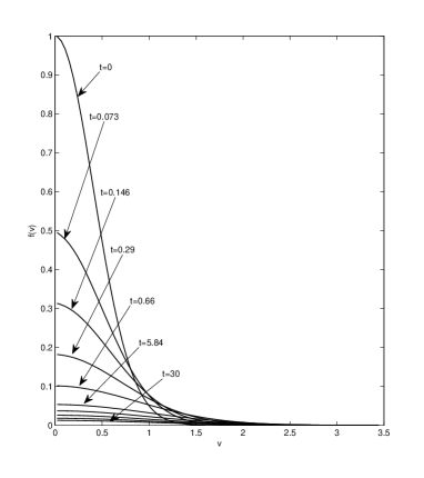
Figure 1: Velocity distribution $f(v,t)$ at different times. The parameters are $d=3$, $D=1$, $\beta=1$, $R=2\sqrt{3}$. The initial distribution is $f_{0}(v)=e^{-3v^{2}}$ for $v\leq 1$ and $f_{0}(v)=0$ for $v>1$. Due to evaporation, the distribution function decreases and tends to zero for $t\rightarrow+\infty$.

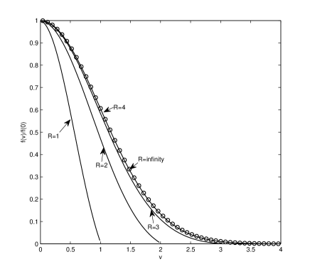
Figure 2: Normalized velocity profile $f(v)/f(0)$ at large times (eigenfunction) for different values of $R$. The slope at the escape velocity $v=R$ decreases as $R$ increases leading to slower mass loss. For $R\rightarrow+\infty$, the distribution function tends to the Maxwellian (bullets).

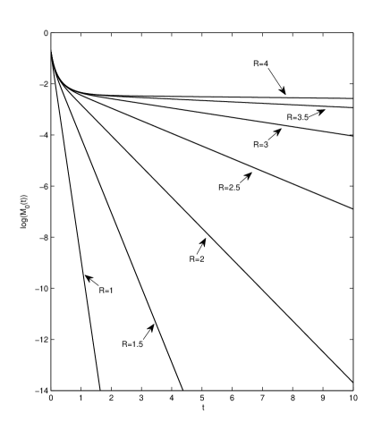
Figure 3: Decay of the mass $M_{0}(t)$ contained in the cluster as a function of time (logarithmic scale). For large times, the decay is exponential $M_{0}(t)\sim e^{-|\lambda(R)|t}$ leading to straight lines with slope $\lambda(R)$. The exponential decay rate $|\lambda(R)|$ decreases as $R$ increases.

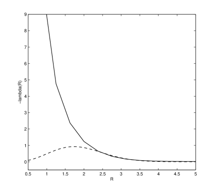
Figure 4: Mass decay rate $|\lambda(R)|$ (eigenvalue) for different values of $R$. The decay rate tends to $+\infty$ for $R\rightarrow 0$ and is equivalent to the asymptotic expression (2.13) for $R\rightarrow+\infty$.

In Fig. 1, we show the velocity distribution $f(v,t)$ at different times. We have adopted the value $R=2\sqrt{3}$ of the escape velocity corresponding to the estimate deduced from the virial theorem (see Introduction). The initial distribution is $f_{0}(v)=e^{-3v^{2}}$ for $v\leq 1$ and $f_{0}(v)=0$ for $v>1$. Due to evaporation, the distribution function decreases and tends to zero for $t\rightarrow+\infty$. In fact, its large time behavior is of the form $f(v,t)\sim e^{-|\lambda(R)|t}f_{\lambda}(v)$. If we rescale the distribution $f(v,t)$ by its central value $f(0,t)$, then the normalized velocity profile $f(v,t)/f(0,t)$ tends to the eigenfunction $f_{\lambda}(v)/f_{\lambda}(0)$. This eigenfunction is represented in Fig. 2 for different values of $R$. We see that the slope of the distribution at the escape velocity $R$ decreases as $R$ increases implying a slower mass loss. In fact, for $R\rightarrow+\infty$, the mass loss tends to zero and the eigenfunction tends to the Maxwellian which is the steady state of the Kramers equation without velocity confinement. In Fig. 3, we plot the mass $M_{0}(t)$ contained in the cluster as a function of time in logarithmic scale. For large times, the decay is exponential $M_{0}(t)\sim e^{-|\lambda(R)|t}$ leading to straight lines with slope $\lambda(R)$. The exponential decay rate $|\lambda(R)|$ decreases as $R$ increases. This decay rate is plotted in Fig. 4 for different values of $R$. The decay rate tends to $+\infty$ for $R\rightarrow 0$ and behaves like (2.13) for $R\rightarrow+\infty$.

4 Conclusion

In this paper, we have obtained new analytical results for the escape of stars from globular clusters in the framework of the Chandrasekhar model. These results can also have applications to other physical systems described by the Kramers equation with parabolic potential and absorbing boundary conditions (i.e. the classical Kramers problem).

We have first obtained an autonomous equation for the mass loss [see (2.6)] and a semi-explicit expression of the distribution function $f(v,t)$ [see (2.4)] that are valid for an arbitrary escape velocity $R$ and time $t$. We have simplified the expression of the mass loss in the limit $R\rightarrow+\infty$ for any fixed time $t$ [see (2.7)]. We have also used the semi-explicit expression of the distribution function $f(v,t)$ to obtain an exact integral equation for the fundamental eigenvalue $\lambda(R)$ [see (2.10)] and for the fundamental eigenfunction $f_{\lambda}(v)$ [see (2.12)] that are valid for any sufficiently large $R$. This is an interesting complement to the perturbative results derived by Chandrasekhar [1] that are valid in the asymptotic limit $R\rightarrow+\infty$. We have obtained the explicit behavior of the fundamental eigenvalue in the limit $R\rightarrow+\infty$ [see (2.13)] which improves upon the result of Chandrasekhar expressed in the form of a series. Additional asymptotic results for the fundamental eigenvalue and fundamental eigenfunction are given in Appendix D. Finally, we have illustrated our results with numerical simulations [see Sec. 3].

Of course, our approach is based on several approximations. As previously discussed, it assumes that the medium is infinite and spatially homogeneous and that the encounters between stars can be described by the Kramers equation (Chandrasekhar’s model). Furthermore, our analytical results (except those of Appendix D) are valid only when the diffusion coefficient in the Fokker-Planck equation is constant while a more exact description of encounters between stars would involve a velocity dependent diffusion coefficient [5, 7, 8]. It remains therefore a challenging issue to extend the mathematical theory of the escape of stars from globular clusters in the case of more realistic models.

Acknowledgement.  M. Lemou was supported by the French Agence Nationale de la Recherche, ANR JC MNEC.

Appendix

A Proof of Proposition 2.1

We consider the Fokker-Planck equation (2.3) with $D=1$. We recall that the initial data is assumed to be isotropic (i.e. it depends on the modulus of the velocity only), which implies that the solution $f(v,t)$ is isotropic at any time.

First we claim that if $f$ is a solution to (2.3) on the ball $B_{R}$ with a vanishing boundary condition, then $f$ is a solution on all ${\mathbb{R}}^{d}$ in a distributional sense to

$$\frac{\partial f}{\partial t}(v,t)=\nabla\cdot\left(\nabla f(v)+\beta f(v)v\right)+M_{0}^{\prime}(t)\frac{\delta_{{\mathbb{S}}_{R}^{d}}}{|{\mathbb{S}}_{R}^{d}|},$$ (A.14)

where $M_{0}$ is related to $f$ by (2.5) and $\delta_{{\mathbb{S}}_{R}^{d}}$ is the Dirac operator on the sphere:

$$<\delta_{{\mathbb{S}}_{R}^{d}},\phi>=\int_{{\mathbb{S}}_{R}^{d}}\phi(v)d\sigma(v),$$

for all test function $\phi$. Note that on isotropic test functions $\phi$, this Dirac operator reduces to: $<\delta_{{\mathbb{S}}_{R}^{d}},\phi>=|{\mathbb{S}}_{R}^{d}|\phi(R)$.

To prove (A.14), consider an isotropic solution $f$ to (2.3) which we extend to $0$ outside $B_{R}$, and integrate (2.3) against an isotropic test function $\phi$ on ${\mathbb{R}}^{d}$. We obtain after integration by parts:

$$\frac{d}{dt}\left(\int_{{\mathbb{R}}^{d}}f(v,t)\phi(|v|)dv\right)=\int_{{\mathbb{R}}^{d}}\left(\Delta\phi-{\beta}v\cdot\nabla\phi\right)f(v)dv+\left(\int_{{\mathbb{S}}_{R}^{d}}\nabla f\cdot n\ d\sigma(v)\right)\phi(R).$$

Taking $\phi\equiv 1$ on $B_{R}$, we also have

$$M_{0}^{\prime}(t)=\int_{{\mathbb{S}}_{R}^{d}}\nabla f\cdot n\ d\sigma(v).$$

Finally, these last two identities imply that $f$ is a solution to (A.14) in the sense of distributions. Note that the choice of isotropic test functions $\phi$ is sufficient thanks to the radial symmetry of $f$.

Remark: We have shown that the solution of (2.3) is solution of (A.14). This is sufficient for our purposes. However, it is easy to prove that, reciprocally, (A.14) admits an infinity of smooth solutions and that, among all of them, the solution that satisfies $f(R\omega,t)=0$ is the solution of (2.3).

We shall now use Fourier transform techniques to find out a semi-explicit solution to (A.14). Let ${\hat{f}}(\xi,t)$ be the Fourier transform of $f$ in the $v$ variable:

$${\hat{f}}(\xi,t)=\int_{{\mathbb{R}}^{d}}f(v,t){\rm exp}(-iv\cdot\xi)\,dv,$$

$$f(v,t)=\int_{{\mathbb{R}}^{d}}{\hat{f}}(\xi,t){\rm exp}(iv\cdot\xi)\,\frac{d\xi}{(2\pi)^{d}}.$$

Taking the Fourier transform in (A.14), we get

$$\frac{\partial{\hat{f}}}{\partial t}(\xi,t)=-\xi^{2}{\hat{f}}-\beta\xi\cdot\nabla{\hat{f}}+M_{0}^{\prime}(t)H(\xi),$$

where

$$H(\xi)=\frac{1}{|{\mathbb{S}}_{R}^{d}|}\int_{{\mathbb{S}}_{R}^{d}}{\rm exp}(-iv\cdot\xi)\,d\sigma({v}).$$

We now use the method of characteristics to solve this equation. Let

$$F(\xi,t)={\hat{f}}(\xi{\rm exp}(\beta t),t).$$

Easy computations yield

$$\frac{\partial F}{\partial t}(\xi,t)=-\xi^{2}{\rm exp}(2\beta t)F(\xi,t)+M_{0}^{\prime}(t)H(\xi{\rm exp}(\beta t)).$$

This can be written as

$$\frac{\partial}{\partial t}\left({\rm exp}\left(\frac{\xi^{2}}{2\beta}({\rm exp}(2\beta t)-1)\right)F(\xi,t)\right)={\rm exp}\left(\frac{\xi^{2}}{2\beta}({\rm exp}(2\beta t)-1)\right)M_{0}^{\prime}(t)H(\xi{\rm exp}(\beta t)).$$

Integrating over time, we get

$$\begin{array}[]{ll}\displaystyle F(\xi,t)=&{\rm exp}\left(-\frac{\xi^{2}}{2\beta}({\rm exp}(2\beta t)-1)\right)F(\xi,0)\\ &\displaystyle+\int_{0}^{t}{\rm exp}\left(-\frac{\xi^{2}}{2\beta}({\rm exp}(2\beta t)-{\rm exp}(2\beta s))\right)M_{0}^{\prime}(s)H(\xi{\rm exp}(\beta s))ds.\end{array}$$

As ${\hat{f}}(\xi,t)=F(\xi{\rm exp}(-\beta t),t)$, we obtain

$$\begin{array}[]{ll}\displaystyle{\hat{f}}(\xi,t)=&\displaystyle{\rm exp}\left(-\frac{\xi^{2}}{2\beta}(1-{\rm exp}(-2\beta t))\right){\hat{f}}(\xi{\rm exp}(-\beta t),0)\\ &\displaystyle+\int_{0}^{t}{\rm exp}\left(-\frac{\xi^{2}}{2\beta}(1-{\rm exp}({-}2\beta(t-s))\right)M_{0}^{\prime}(s)H(\xi{\rm exp}(-\beta(t-s)))\,ds.\end{array}$$

Using the notations of proposition 2.1, this can also be written as

$${\hat{f}}(\xi,t)={\rm exp}\left(-\xi^{2}A(0,t)\right){\hat{f}}(\xi B(0,t),0)+\int_{0}^{t}{\rm exp}\left(-\xi^{2}A(s,t)\right)M_{0}^{\prime}(s)H(\xi B(s,t))\,ds.$$

Now, we take the inverse Fourier transform using the identities

$${\rm Inv}F\left({\rm exp}(-A\xi^{2})\right)(v)=\frac{1}{(2\pi)^{d}}\left(\frac{\pi}{A}\right)^{d/2}{\rm exp}\left(-\frac{|v|^{2}}{4A}\right),$$

and

$${\rm Inv}F\left({{\rm exp}(-A\xi^{2}){\rm exp}\left(-iB\xi\cdot w\right)}\right)(v)=\frac{1}{(2\pi)^{d}}\left(\frac{\pi}{A}\right)^{d/2}{\rm exp}\left(-\frac{|Bw-v|^{2}}{4A}\right),$$

to get the desired expression (2.4).

Remark: if we integrate (2.4) on the velocity, we find a trivial result: $M_{0}(t)=M_{0}(t)$, which shows the consistency of this equation.

B Proof of Proposition 2.2

Let $f$ be the solution to (2.3) with initial data $f_{0}$ and let $M_{0}$ be defined by (2.5). From (2.4) and the vanishing boundary condition $f(R\omega,t)=0,$ $\omega\in{S_{1}^{d}},$ we get

$$T_{1}+T_{2}=0,$$ (B.15)

where

$$T_{1}=|{\mathbb{S}}_{1}^{d}|A(0,t)^{-d/2}\int_{{\mathbb{R}}^{d}}f_{0}(v_{*})\,{\rm exp}\left(-\frac{|R\omega-B(0,t)v_{*}|^{2}}{4A(0,t)}\right)\,dv_{*},$$ (B.16)

$$T_{2}=\int_{0}^{t}dsA(s,t)^{-d/2}M_{0}^{\prime}(s)\int_{\sigma\in{\mathbb{S}}_{1}^{d}}{\rm exp}\left(-\frac{R^{2}|B(s,t)\sigma+\omega|^{2}}{4A(s,t)}\right)\,{d\sigma},$$ (B.17)

where $A$ and $B$ are defined in proposition 2.1.

To analyze the asymptotic behavior of the term $T_{1}$ when $R$ goes to $+\infty$, the time $t$ being fixed, we introduce a spherical system of coordinates (in ${\mathbb{R}}^{d}$), write $v_{*}=r\sigma$, $\sigma\in{\mathbb{S}}_{1}^{d}$, $\sigma\cdot\omega=\cos\theta$ and obtain

$$\begin{array}[]{ll}\displaystyle T_{1}&\displaystyle=|{\mathbb{S}}_{1}^{d}|A(0,t)^{-d/2}\int_{0}^{+\infty}\int_{0}^{\pi}f_{0}(r)\\ \displaystyle&\displaystyle\times{\rm exp}\left(-\frac{R^{2}-2RB(0,t)r\cos\theta+B(0,t)^{2}r^{2}}{4A(0,t)}\right)\,C_{d}r^{d-1}dr(\sin\theta)^{d-2}d\theta,\end{array}$$

where $C_{d}$ is given by

$$C_{d}=\frac{|{\mathbb{S}}_{1}^{d}|}{\displaystyle\int_{0}^{\pi}(\sin\theta)^{d-2}d\theta},\ \ \ d\geq 2.$$ (B.18)

In the following calculations, we shall assume $d\geq 2$ but we have checked by a specific calculation that the final result remains valid for $d=1$. Making the change of variable $\delta=-\cos\theta$, we obtain

$$\begin{array}[]{ll}\displaystyle T_{1}=&\displaystyle C_{d}|{\mathbb{S}}_{1}^{d}|A(0,t)^{-d/2}{\rm exp}\left(-\frac{R^{2}}{4A(0,t)}\right)\\ &\displaystyle\times\int_{0}^{+\infty}\int_{-1}^{1}f_{0}(r)\,{\rm exp}\left(-\frac{B(0,t)^{2}}{4A(0,t)}r^{2}\right){\rm exp}\left(-\frac{B(0,t)}{2A(0,t)}Rr\delta\right)r^{d-1}\left(1-\delta^{2}\right)^{\frac{d-3}{2}}\,d\delta dr.\end{array}$$

We then make the change of variable $u=\frac{B(0,t)}{2A(0,t)}Rr(1+\delta)$ in the integral over $\delta$, and get

$$\begin{array}[]{ll}\displaystyle&\displaystyle T_{1}=C_{d}2^{d-2}|{\mathbb{S}}_{1}^{d}|A(0,t)^{-d/2}\left(\frac{A(0,t)}{B(0,t)R}\right)^{\frac{d-1}{2}}\\ &\displaystyle\times\int_{0}^{+\infty}\int_{0}^{\frac{B(0,t)}{A(0,t)}Rr}f_{0}(r)\,{\rm exp}\left(-\frac{(B(0,t)r-R)^{2}}{4A(0,t)}\right)\left(1-\frac{A(0,t)}{B(0,t)R}\frac{u}{r}\right)^{\frac{d-3}{2}}r^{\frac{d-1}{2}}u^{\frac{d-3}{2}}{\rm exp}(-u)\,dudr.\end{array}$$

Now let $R$ go to infinity to obtain

$$\begin{array}[]{ll}\displaystyle T_{1}\ \sim\ C_{d}2^{{d-2}}|{\mathbb{S}}_{1}^{d}|&\displaystyle\Gamma\left(\frac{d-1}{2}\right)A(0,t)^{-d/2}\left(\frac{A(0,t)}{B(0,t)R}\right)^{\frac{d-1}{2}}\\ &\displaystyle\times\int_{0}^{+\infty}f_{0}(r)\,{\rm exp}\left(-\frac{(B(0,t)r-R)^{2}}{4A(0,t)}\right)r^{\frac{d-1}{2}}\,dr,\end{array}$$ (B.19)

as $R$ goes to $+\infty$.

Assume first that $f_{0}$ does not depend on $R$ and is supported on $[0,R_{0}]$. In that case, we perform the change of variable:

$$s=\frac{B(0,t)R}{2A(0,t)}(R_{0}-{r}),$$

and get

$$\begin{array}[]{ll}\displaystyle&\displaystyle\int_{0}^{+\infty}\displaystyle f_{0}(r)\,{\rm exp}\left(-\frac{(B(0,t)r-R)^{2}}{4A(0,t)}\right)r^{\frac{d-1}{2}}\,dr\ =\ \frac{2A(0,t)}{B(0,t)R}\,{\rm exp}\left(-\frac{(B(0,t)R_{0}-R)^{2}}{4A(0,t)}\right)\\ &\displaystyle\times\int_{0}^{\frac{B(0,t)RR_{0}}{2A(0,t)}}f_{0}\left(R_{0}-\frac{2A(0,t)}{B(0,t)R}s\right){\rm exp}\left(-s+\frac{B(0,t)R_{0}}{R}s-\frac{A(0,t)}{R^{2}}s^{2}\right)\left(R_{0}-\frac{2A(0,t)}{B(0,t)R}s\right)^{\frac{d-1}{2}}\,ds.\end{array}$$

If we let $R$ go to infinity in this expression, then we obtain

$$\begin{array}[]{ll}\displaystyle\int_{0}^{+\infty}f_{0}(r)&\displaystyle{\rm exp}\left(-\frac{(B(0,t)r-R)^{2}}{4A(0,t)}\right)r^{\frac{d-1}{2}}\,dr\ \sim\\ &\displaystyle\ -\left(\frac{2A(0,t)}{B(0,t)R}\right)^{2}{\rm exp}\left(-\frac{(B(0,t)R_{0}-R)^{2}}{4A(0,t)}\right)R_{0}^{\frac{d-1}{2}}f_{0}^{\prime}(R_{0}),\end{array}$$ (B.20)

for large $R$. The case where $f_{0}$ does depend on $R$ can be treated similarly to yield

$$\begin{array}[]{ll}\displaystyle\int_{0}^{+\infty}f_{0}(r)&\displaystyle{\rm exp}\left(-\frac{(B(0,t)r-R)^{2}}{4A(0,t)}\right)r^{\frac{d-1}{2}}\,dr\ \sim\\ &\displaystyle-\left(\frac{2A(0,t)}{B(0,t)R}\right)^{2}{\rm exp}\left(-\frac{(1-B(0,t))^{2}}{4A(0,t)}R^{2}\right)\frac{R^{\frac{d-1}{2}}}{[1-B(0,t)]^{2}}f_{0}^{\prime}(R),\end{array}$$ (B.21)

for large $R$. We now deal with the asymptotic behavior of the term $T_{2}$ given by (B.17) when $R$ goes to $+\infty$. First, we write $T_{2}$ in the following form

$$T_{2}=\int_{0}^{t}dsA(s,t)^{-d/2}M_{0}^{\prime}(s){\rm exp}\left(-\frac{R^{2}(B(s,t)^{2}+1)}{4A(s,t)}\right)\int_{\sigma\in{\mathbb{S}}_{1}^{d}}{\rm exp}\left(-\frac{R^{2}B(s,t)}{2A(s,t)}\sigma\cdot\omega\right)\,d\sigma.$$

We then introduce spherical coordinates (in ${\mathbb{R}}^{d}$) in the variable $\sigma\in{\mathbb{S}}_{1}^{d}$ and obtain

$$T_{2}=C_{d}\int_{0}^{t}dsA(s,t)^{-d/2}M_{0}^{\prime}(s){\rm exp}\left(-\frac{R^{2}(B(s,t)^{2}+1)}{4A(s,t)}\right)\int_{0}^{\pi}{\rm exp}\left(-\frac{R^{2}B(s,t)}{2A(s,t)}\cos\theta\right)(\sin\theta)^{d-2}\,d\theta.$$

Performing the change of variable $u=\frac{R^{2}B(s,t)}{2A(s,t)}(1+\cos\theta)$ in the integral over $\theta$, we get

$$\begin{array}[]{ll}\displaystyle T_{2}=C_{d}2^{{d-2}}\int_{0}^{t}dsA(s,t)^{-d/2}M_{0}^{\prime}(s)&\displaystyle\left(\frac{A(s,t)}{R^{2}B(s,t)}\right)^{\frac{d-1}{2}}{\rm exp}\left(-\frac{R^{2}(B(s,t)-1)^{2}}{4A(s,t)}\right)\\ &\displaystyle\times\int_{0}^{\frac{R^{2}B(s,t)}{A(s,t)}}\left(1-\frac{A(s,t)}{R^{2}B(s,t)}u\right)^{\frac{d-3}{2}}u^{\frac{d-3}{2}}{\rm exp}(-u)\,du.\end{array}$$

Letting $R\rightarrow+\infty$, we have

$$T_{2}\ \sim\ C_{d}2^{d-2}\Gamma\left(\frac{d-1}{2}\right)\int_{0}^{t}A(s,t)^{-d/2}M_{0}^{\prime}(s)\left(\frac{A(s,t)}{R^{2}B(s,t)}\right)^{\frac{d-1}{2}}{\rm exp}\left(-\frac{R^{2}(B(s,t)-1)^{2}}{4A(s,t)}\right)\,ds.$$

We now use the following change of variable in this last integral over $s$:

$$\tau=\frac{1-B(s,t)}{2\sqrt{A(s,t)}}R=\left(\frac{\beta}{2}\frac{1-{\rm exp}(-\beta(t-s))}{1+{\rm exp}(-\beta(t-s))}\right)^{1/2}R,$$

to obtain

$$\begin{array}[]{ll}\displaystyle T_{2}\ \sim\ C_{d}2^{d-2}&\displaystyle\Gamma\left(\frac{d-1}{2}\right)\frac{4}{\beta}R^{-d}\int_{0}^{R\left(\frac{\beta(1-{\rm exp}(-\beta t))}{2(1+{\rm exp}(-\beta t))}\right)^{1/2}}\left(1-\frac{2\tau^{2}}{\beta R^{2}}\right)^{-(d+1)/2}\left(1+\frac{2\tau^{2}}{\beta R^{2}}\right)^{\frac{d-1}{2}}\\ &\displaystyle M_{0}^{\prime}\left(t+\frac{1}{\beta}\ln\left(\frac{\beta R^{2}-2\tau^{2}}{\beta R^{2}+2\tau^{2}}\right)\right){\rm exp}(-\tau^{2})\,d\tau.\end{array}$$

This yields an equivalent of $T_{2}$

$$T_{2}\ \sim\ C_{d}2^{{d-1}}\Gamma\left(\frac{d-1}{2}\right)\frac{\sqrt{\pi}}{\beta R^{d}}M_{0}^{\prime}(t),$$ (B.22)

for large $R$.

Combining (B.15) with (B.19) and (B.22) leads to the result (2.7) of proposition 2.2. Finally, substituting (B.20) (resp. (B.21)) into (2.7) yields (2.8) (resp. (2.9)).

C Proof of proposition 2.3

We first prove i) in proposition 2.3. We shall use the exact solution (2.4) stated in proposition 2.1. Let $\lambda$ be the fundamental (largest non zero) eigenvalue of the Fokker-Planck operator (2.3). Even if the proof of $\lambda<0$ is classical, we give the argument here for the sake of completeness. If $f$ is an associated eigenfunction, the eigenvalue problem can be written as

$$\nabla\cdot\left[D(|v|){\rm exp}(-\beta|v|^{2}/2)\nabla\left(f(v){\rm exp}(\beta|v|^{2}/2)\right)\right]=\lambda f.$$

Integrating against $f(v){\rm exp}(\beta|v|^{2}/2)$ on $B_{R}$, we get

$$-\int_{B_{R}}D(|v|){\rm exp}(-\beta|v|^{2}/2)\left|\nabla\left(f(v){\rm exp}(\beta|v|^{2}/2)\right)\right|^{2}dv=\lambda\int_{B_{R}}f(v)^{2}{\rm exp}(\beta|v|^{2}/2)dv,$$

which implies that $\lambda<0$. We now prove relation (2.10). Let $f_{\lambda}(v)$ be an eigenfunction associated to $\lambda$, then ${\rm exp}(\lambda t)f_{\lambda}(v)$ is the solution of (2.3) with initial data $f_{\lambda}$. Therefore, using (2.4), the eigenvalue problem can be written as

$${\rm exp}(\lambda t)f_{\lambda}(v)=T_{1}(f_{\lambda})(v,t)+\lambda M_{\lambda}\int_{0}^{t}G(v,{\rm exp}(-\beta(t-s)){\rm exp}(\lambda s)\,ds,$$

where $G$ is given by (2.11), $M_{\lambda}=\int_{B_{R}}f_{\lambda}(v)dv$ and

$$T_{1}(f_{\lambda})(v,t)=\frac{1}{(2\pi)^{d}}\left(\frac{\pi}{A(0,t)}\right)^{d/2}\int_{{B_{R}}}f_{\lambda}(v_{*}){\rm exp}\left(-\frac{|v-v_{*}B(0,t)|^{2}}{4A(0,t)}\right)dv_{*}.$$ (C.23)

This relation can be rewritten equivalently

$$\begin{array}[]{ll}\displaystyle{\rm exp}(\lambda t)f_{\lambda}(v)&\displaystyle=T_{1}(f_{\lambda})(v,t)-M_{\lambda}G(v,0)+M_{\lambda}G(v,0){\rm exp}(\lambda t)\\ &\displaystyle{+}\lambda M_{\lambda}\int_{0}^{t}\left[G(v,{\rm exp}(-\beta(t-s))-G(v,0)\right]{\rm exp}(\lambda s)ds,\ \ \forall t\geq 0.\end{array}$$ (C.24)

We now analyze this relation for large time $t$. First, we expand the term $T_{1}(f_{\lambda})(v,t)$ and obtain after easy computations:

$$\begin{array}[]{ll}\displaystyle&T_{1}(f_{\lambda})(v,t)=\displaystyle{G(v,0)\left[M_{\lambda}+\beta v\cdot\left(\int v_{*}f_{\lambda}(v_{*})dv_{*}\right){\rm exp}(-\beta t)+\frac{1}{2}(d-\beta v^{2})M_{\lambda}{\rm exp}(-2\beta t)\right.}\\ &{\left.\displaystyle-\frac{1}{2}\beta\left(\int|v_{*}|^{2}f_{\lambda}(v_{*})dv_{*}\right){\rm exp}(-2\beta t)+\frac{1}{2}\beta^{2}\left(\int(v\cdot v_{*})^{2}f_{\lambda}(v_{*})dv_{*}\right){\rm exp}(-2\beta t)\right]+O({\rm exp}(-3\beta t)).}\end{array}$$

As $f_{\lambda}$ is supposed to be radially symmetric in $v$, the order 1 contribution in ${\rm exp}(-\beta t)$ vanishes, and we get after some rearrangements

$$\begin{array}[]{ll}\displaystyle T_{1}(f_{\lambda})(v,t)=\displaystyle G(v,0)\left[M_{\lambda}+\frac{1}{2}(d-\beta v^{2})\left(M_{\lambda}-\frac{\beta}{d}\int|v_{*}|^{2}f_{\lambda}(v_{*})dv_{*}\right){\rm exp}(-2\beta t)\right]\\ \displaystyle+O({\rm exp}(-3\beta t)).\end{array}$$

This implies in particular that

$$\mathop{\rm lim}_{t\rightarrow+\infty}{\rm exp}(2\beta t)\left[T_{1}(f_{\lambda})(v,t)-M_{\lambda}G(v,0)\right]$$

is finite. Now we multiply (C.24) by ${\rm exp}(2\beta t)$ and perform the change of variable $u={\rm exp}(-\beta(t-s))$ in the rhs of (C.24) to obtain

$$\begin{array}[]{ll}\displaystyle{\rm exp}\left((\lambda+2\beta)t\right)f_{\lambda}(v)&={\rm exp}(2\beta t)\left[T_{1}(f_{\lambda})(v,t)-\right.\left.M_{\lambda}G(v,0)\right]+\displaystyle M_{\lambda}{\rm exp}\left((\lambda+2\beta)t\right)\\ &\displaystyle\times\left[G(v,0)+\frac{\lambda}{\beta}\int_{{\rm exp}(-\beta t)}^{1}\left(G(v,u)-G(v,0)\right)u^{\frac{\lambda}{\beta}-1}du\right].\end{array}$$ (C.25)

Before taking the limit $t\rightarrow+\infty$, we first claim that

$$\lambda+2\beta>0,$$

at least for large enough $R$. Indeed, we know that if $R=+\infty$, $0$ is an eigenvalue of the Fokker-Planck operator (2.3). Therefore, the first eigenvalue $\lambda(R)$ on $B_{R}$ must go to $0$ when $R$ goes to infinity, and this proves the claim. Passing to the limit $t\rightarrow+\infty$ in (C.25), we conclude that we necessarily have

$$f_{\lambda}(v)=M_{\lambda}\left\{G(v,0)+\frac{\lambda}{\beta}\int_{0}^{1}\left[G(v,u)-G(v,0)\right]u^{\frac{\lambda}{\beta}-1}du\right\},$$

which is relation (2.12). Finally, writing this relation at the boundary $v=R\omega$, $\omega\in{\mathbb{S}}_{1}^{d}$, and recalling that $f_{\lambda}(R\omega)=0$, we get

$$G(R\omega,0)+\frac{\lambda}{\beta}\int_{0}^{1}\left[G(R\omega,u)-G(R\omega,0)\right]u^{\frac{\lambda}{\beta}-1}du=0,$$

which is relation (2.10).

We now prove the asymptotic behavior (2.13) for large $R$. As $\lambda(R)$ goes to $0$ when $R$ goes to infinity and

$$G(R\omega,0)=\frac{1}{(2\pi)^{d}}({2\pi\beta})^{d/2}{\rm exp}\left(-\beta\frac{R^{2}}{2}\right),$$

we obtain

$$\begin{array}[]{ll}\displaystyle{\rm exp}\left(-\beta\frac{R^{2}}{2}\right)\sim-\frac{\lambda}{\beta}\frac{1}{|{\mathbb{S}}_{1}^{d}|}\int_{{\mathbb{S}}_{1}^{d}}d\sigma\int_{0}^{1}\left[(1-u^{2})^{-d/2}{\rm exp}\left(-\frac{\beta R^{2}}{2}\frac{|\sigma u+\omega|^{2}}{1-u^{2}}\right)-{\rm exp}\left(-\beta\frac{R^{2}}{2}\right)\right]\frac{du}{u}.\end{array}$$

This is also equivalent to

$$\lambda(R)\sim-\frac{\beta|{\mathbb{S}}_{1}^{d}|}{I_{d}(R)},$$ (C.26)

where

$$I_{d}(R)=\int_{{\mathbb{S}}_{1}^{d}}d\sigma\int_{0}^{1}\left[(1-u^{2})^{-d/2}{\rm exp}\left(-\beta R^{2}\frac{u(u+\sigma\cdot\omega)}{1-u^{2}}\right)-1\right]\frac{du}{u}.$$ (C.27)

Now we write

$$I_{d}(R)=I_{d}^{+}(R)+I_{d}^{-}(R),$$

with

$$I_{d}^{+}(R)=\int_{{\mathbb{S}}^{+}}d\sigma\int_{0}^{1}\left[(1-u^{2})^{-d/2}{\rm exp}\left(-\beta R^{2}\frac{u(u+\sigma\cdot\omega)}{1-u^{2}}\right)-1\right]\frac{du}{u},$$

and $I_{d}^{-}(R)=I_{d}(R)-I_{d}^{+}(R)$, ${\mathbb{S}}^{+}=\{\sigma\in{\mathbb{S}}_{1}^{d},\sigma\cdot\omega>0\}$,  ${\mathbb{S}}^{-}={\mathbb{S}}_{1}^{d}-{\mathbb{S}}^{+}$. First, we show that $R^{-2}I_{d}^{+}(R)$ is uniformly bounded in $R$. Indeed, we have

$$|I_{d}^{+}(R)|\leq{\frac{|{\mathbb{S}}_{1}^{d}|}{2}}\int_{0}^{1}\left|(1-u^{2})^{-d/2}{\rm exp}\left(-\beta R^{2}\frac{u^{2}}{1-u^{2}}\right)-1\right|\frac{du}{u},$$

and the change of variable

$$s^{2}=\beta R^{2}\frac{u^{2}}{1-u^{2}},$$

leads to

$${|I_{d}^{+}(R)|\leq\frac{|{\mathbb{S}}_{1}^{d}|}{2}\int_{0}^{+\infty}\left|\left(1+\frac{s^{2}}{\beta R^{2}}\right)^{d/2}{\rm exp}(-s^{2})-1\right|\frac{ds}{s(\frac{s^{2}}{\beta R^{2}}+1)}.}$$

A simple computation of the derivative of the function

$$\theta(s)=1-\left(1+\frac{s^{2}}{\beta R^{2}}\right)^{d/2}{\rm exp}(-s^{2}),$$

shows that it is an increasing function on $[0,+\infty[$, for large enough $R$ ($R>\sqrt{d/2\beta}$). Therefore, it is a non-negative function on $[0,+\infty[$, and consequently

$${|I_{d}^{+}(R)|\leq\frac{|{\mathbb{S}}_{1}^{d}|}{2}\int_{0}^{+\infty}\left(\frac{1-{\rm exp}(-s^{2})}{s}\right)\frac{ds}{\frac{s^{2}}{\beta R^{2}}+1}.}$$

This clearly shows that $R^{-2}I_{d}^{+}(R)$ is uniformly bounded for large $R$.

We now focus on the behavior of $I_{d}^{-}(R)$ when $R$ goes to infinity and let $\delta=-\sigma\cdot\omega$ and

$$S_{\delta}(u)=\frac{u(\delta-u)}{1-u^{2}}.$$ (C.28)

Then, we have

$$I_{d}^{-}(R)=\int_{{\mathbb{S}}^{-}}d\sigma\int_{0}^{1}\left[(1-u^{2})^{-d/2}{\rm exp}\left(\beta R^{2}S_{\delta}(u)\right)-1\right]\frac{du}{u}.$$ (C.29)

We now show that the dominant part in $I_{d}^{-}(R)$ is given by the contribution at ${u=u_{\delta}}$, where ${u_{\delta}}$ is such that

$$\max_{u\in[0,1]}S_{\delta}(u)=S_{\delta}(u_{\delta}).$$

We first have

$$u_{\delta}=\frac{1}{\delta}\left(1-\sqrt{1-\delta^{2}}\right),\ \ \ \ S_{\delta}(u_{\delta})=\frac{1}{2}\left(1-\sqrt{1-\delta^{2}}\right),$$

and observe that

$$S_{\delta}(u)-S_{\delta}(u_{\delta})=-\frac{\left(\delta u-1+\sqrt{1-\delta^{2}}\right)^{2}}{2(1-u^{2})\left(1-\sqrt{1-\delta^{2}}\right)}.$$

Thus, from (C.29)

$$\begin{array}[]{ll}\displaystyle I_{d}^{-}(R)=&\displaystyle{\rm exp}\left(\frac{\beta R^{2}}{2}\right)\int_{{\mathbb{S}}^{-}}d\sigma\,{\rm exp}\left(-\frac{\beta R^{2}}{2}\sqrt{1-\delta^{2}}\right)\\ &\displaystyle\times\int_{0}^{1}\left[(1-u^{2})^{-d/2}{\rm exp}\left(-\beta R^{2}\frac{\delta\left(u-u_{\delta}\right)^{2}}{2u_{\delta}(1-u^{2})}\right)-{\rm exp}\left(-\frac{\beta R^{2}}{2}\delta u_{\delta}\right)\right]\frac{du}{u}.\end{array}$$ (C.30)

We now introduce a spherical system of coordinates (in ${\mathbb{R}}^{d}$) for the integration on the sphere and use identity

$${\int_{{\mathbb{S}}^{-}}F(-\sigma\cdot\omega)d\sigma=C_{d}\int_{\frac{\pi}{2}}^{\pi}F(-\cos\theta)(\sin\theta)^{d-2}d\theta=C_{d}\int_{0}^{1}F(\delta)(1-\delta^{2})^{\frac{d-3}{2}}d\delta,}$$

where $F$ is a real function and $C_{d}$ is given by (B.18). In the following, we assume $d\geq 2$ but we have checked by a specific calculation that the results remain valid for $d=1$. Using this identity in (C.30), we get

$$\begin{array}[]{ll}\displaystyle I_{d}^{-}(R)=&\displaystyle C_{d}{\rm exp}\left(\frac{\beta R^{2}}{2}\right)\int_{0}^{1}d\delta\ (1-\delta^{2})^{\frac{d-3}{2}}{\rm exp}\left(-\frac{\beta R^{2}}{2}\sqrt{1-\delta^{2}}\right)\\ &\displaystyle{\times\int_{0}^{1}}\left[(1-u^{2})^{-d/2}{\rm exp}\left(-\beta R^{2}\frac{\delta\left(u-u_{\delta}\right)^{2}}{2u_{\delta}(1-u^{2})}\right)-{\rm exp}\left(-\frac{\beta R^{2}}{2}\delta u_{\delta}\right)\right]\frac{du}{u}.\end{array}$$ (C.31)

We now perform the following change of variables in (C.31) for both $\delta$ and $u$

$$t=\frac{u-u_{\delta}}{\sqrt{1-u^{2}}}\left(\frac{\beta R^{2}}{2}\frac{\delta}{u_{\delta}}\right)^{1/2},\ \ \ r=\left(\frac{\beta R^{2}}{2}\right)^{1/2}(1-\delta^{2})^{1/4},$$

which is also equivalent to

$$u=u(t,r)=\frac{(a^{2}-r^{4})^{1/2}+t(t^{2}+2r^{2})^{1/2}}{a+r^{2}+t^{2}},\ \ \ \ \delta=\left(1-\frac{r^{4}}{a^{2}}\right)^{1/2},$$ (C.32)

with $a=\beta R^{2}/2.$ After some calculations, we get from (C.31)

$$\begin{array}[]{ll}\displaystyle&\displaystyle I_{d}^{-}(R)=2C_{d}\left(\frac{2}{\beta R^{2}}\right)^{d-\frac{1}{2}}{\rm exp}\left(\frac{\beta R^{2}}{2}\right)\int_{0}^{{\sqrt{a}}}dr\,r^{2d-3}\left(1-\frac{r^{4}}{a^{2}}\right)^{-1/2}\int_{-(a-r^{2})^{1/2}}^{+\infty}dt\\ &\displaystyle\times\left[(1-u(t,r)^{2})^{-d/2}{\rm exp}(-r^{2}-t^{2})-{\rm exp}\left(-a\right)\right]\frac{(1-u(t,r)^{2})^{3/2}}{\left(1+\frac{r^{2}}{a}\right)^{1/2}u(t,r)(1-u(t,r)u_{\delta}(r))}.\end{array}$$ (C.33)

We now want to analyze the asymptotic behavior of (C.33) when $a=\beta R^{2}/2$ goes to infinity. Thanks to the strong decreasing properties of ${\rm exp}(-t^{2}-r^{2})$, one can expand the terms inside the integral in the limit $a\rightarrow+\infty$. To do so, we first obtain from easy calculations

$$1-u(t,r)=\frac{1}{a}\left[r^{2}+t^{2}-t(t^{2}+2r^{2})^{1/2}\right]+O\left(\frac{1}{a^{2}}\right)=\frac{1}{2a}\left[(t^{2}+2r^{2})^{1/2}-t\right]^{2}+O\left(\frac{1}{a^{2}}\right),$$

and

$$1-u(t,r)u_{\delta}(r)=\frac{1}{a}(t^{2}+2r^{2})^{1/2}\left[(t^{2}+2r^{2})^{1/2}-t\right]+O\left(\frac{1}{a^{2}}\right).$$

Then, we plug these relations into (C.33) to obtain

$$\begin{array}[]{ll}\displaystyle I_{d}^{-}(R)\ \sim\ 2C_{d}\left(\frac{\beta R^{2}}{2}\right)^{-d/2}&\displaystyle{\rm exp}\left(\frac{\beta R^{2}}{2}\right)\int_{0}^{+\infty}{dr}\int_{-\infty}^{+\infty}{dt}\\ &\displaystyle\times r^{2d-3}(t^{2}+2r^{2})^{-1/2}{\rm exp}(-r^{2}-t^{2})\left[(t^{2}+2r^{2})^{1/2}-t\right]^{2-d},\end{array}$$ (C.34)

when $a=\beta R^{2}/2$ goes to infinity. To simplify expression (C.34) we perform the cylindrical change of variable: $t=\rho\cos\phi,$ $r=\rho\sin\phi$, with $\phi\in[0,\pi]$, and get

$$\begin{array}[]{ll}\displaystyle I_{d}^{-}(R)\ \sim\ 2^{3-d}C_{d}\left(\frac{\beta R^{2}}{2}\right)^{-d/2}{\rm exp}\left(\frac{\beta R^{2}}{2}\right)&\displaystyle\int_{0}^{+\infty}\rho^{d-1}{\rm exp}(-\rho^{2})\,d\rho\\ &\displaystyle\times\int_{0}^{\pi}\frac{\left[(1+\sin^{2}\phi)^{1/2}+\cos\phi\right]^{d-2}}{(1+\sin^{2}\phi)^{1/2}}{\sin}\phi\,d\phi.\end{array}$$

Performing the change of variable $u=\cos\phi$, we obtain

$$\begin{array}[]{ll}\displaystyle I_{d}^{-}(R)\ \sim\ 2^{2-d}C_{d}\left(\frac{\beta R^{2}}{2}\right)^{-d/2}{\rm exp}\left(\frac{\beta R^{2}}{2}\right)&\displaystyle\Gamma\left(\frac{d}{2}\right)\int_{-1}^{+1}\frac{\left[(2-u^{2})^{1/2}+u\right]^{d-2}}{(2-u^{2})^{1/2}}\,du.\end{array}$$

Performing the change of variable $u=\sqrt{2}\sin t$ in the integral over $u$ we get

$$\int_{-1}^{1}\frac{\left[(2-u^{2})^{1/2}+u\right]^{d-2}}{(2-u^{2})^{1/2}}du=2^{d-2}\int_{-\frac{\pi}{4}}^{\frac{\pi}{4}}\sin^{d-2}\left(t+\frac{\pi}{4}\right)\,dt=2^{d-3}\int_{0}^{\pi}(\sin\phi)^{d-2}d\phi,$$

where we have set $\phi=t+\pi/4$ in the last integral. Using (B.18), we obtain

$$\begin{array}[]{ll}\displaystyle I_{d}^{-}(R)\ \sim\ \frac{1}{2}|{\mathbb{S}}_{1}^{d}|\left(\frac{\beta R^{2}}{2}\right)^{-d/2}{\rm exp}\left(\frac{\beta R^{2}}{2}\right)&\displaystyle\Gamma\left(\frac{d}{2}\right).\end{array}$$

Therefore, $I_{d}^{-}(R)$ increases exponentially rapidly while $I_{d}^{+}(R)$ increases less rapidly than $R^{2}$ and can therefore be neglected. Using (C.26), we finally obtain (2.13). This ends the proof of proposition 2.3.

D Asymptotic expressions of the fundamental eigenfunction and eigenvalue

In this Appendix, we show that the asymptotic result (2.13) can be directly obtained by a perturbative expansion of the solutions of the fundamental eigenvalue equation in powers of $\lambda$ in the limit $\lambda\ll 1$ corresponding to $V\rightarrow+\infty$ (in this Appendix, we introduce more physical notations and set $v=|v|\in{\mathbb{R}}^{+}$ and $V=R\in{\mathbb{R}}^{+}$). This method allows us to treat more general situations, e.g. Fokker-Planck equations with an arbitrary potential $U(v)$ and an arbitrary diffusion coefficient $D(v)$. For the Fokker-Planck equation (2.3) with $U(v)=v^{2}/2$ and $D=1$, we recover (2.13).

For isotropic distributions $f(v,t)$, we consider the Fokker-Planck equation

$${\partial f\over\partial t}={1\over v^{d-1}}{\partial\over\partial v}\biggl{\{}v^{d-1}D(v)\biggl{(}{\partial f\over\partial v}+\beta f{\partial U\over\partial v}\biggr{)}\biggr{\}},$$ (D.35)

where $D(v)$ and $U(v)$ are arbitrary functions of the velocity. We consider the fundamental eigenmode

$$f(v,t)=Ae^{\lambda t}g(v),$$ (D.36)

where $A$ is a normalization constant. We can impose $g(0)=1$ without loss of generality. On the other hand, $g^{\prime}(0)=0$ and $g(V)=0$. Substituting (D.36) in (D.35), we obtain the eigenvalue equation

$$\lambda g={1\over v^{d-1}}{d\over dv}\biggl{\{}v^{d-1}D(v)\biggl{(}{dg\over dv}+\beta g{dU\over\partial v}\biggr{)}\biggr{\}}.$$ (D.37)

It can be integrated into

$${dg\over dv}+\beta g{dU\over\partial v}={\lambda\over v^{d-1}D(v)}\int_{0}^{v}g(w)w^{d-1}dw.$$ (D.38)

For an unlimited range of velocities ($V\rightarrow+\infty$), the Fokker-Planck equation (D.35) admits a steady solution

$$f(v)=\frac{1}{Z}e^{-\beta U(v)},$$ (D.39)

implying that the fundamental eigenvalue is $\lambda(+\infty)=0$. Now for $V<+\infty$, the eigenvalue $\lambda(V)<0$. However, for $V\gg 1$, $\lambda(V)\rightarrow 0^{-}$ and we can formally expand the solution of the differential equation (D.37) in the form

$$g=g_{0}(v)+\lambda g_{1}(v)+\lambda^{2}g_{2}(v)+...$$ (D.40)

To zeroth order, we have

$${dg_{0}\over dv}+\beta g_{0}{dU\over\partial v}=0.$$ (D.41)

To first order in $\lambda$, we get

$${dg_{1}\over dv}+\beta g_{1}{dU\over\partial v}={1\over v^{d-1}D(v)}\int_{0}^{v}g_{0}(w)w^{d-1}dw.$$ (D.42)

With the boundary condition $g_{0}(0)=1$, the first equation can be integrated in

$$g_{0}(v)=e^{-\beta(U(v)-U(0))}.$$ (D.43)

Substituting this expression in (D.42) we obtain

$${dg_{1}\over dv}+\beta g_{1}{dU\over\partial v}={e^{\beta U(0)}\over v^{d-1}D(v)}\int_{0}^{v}e^{-\beta U(w)}w^{d-1}dw,$$ (D.44)

that we shall solve with the boundary conditions $g_{1}(0)=g^{\prime}_{1}(0)=0$. We obtain

$$g_{1}(v)=\chi(v)e^{-\beta(U(v)-U(0))},$$ (D.45)

where $\chi(v)$ is the function defined by

$$\chi^{\prime}(v)={e^{\beta U(v)}\over v^{d-1}D(v)}\int_{0}^{v}e^{-\beta U(w)}w^{d-1}dw,$$ (D.46)

with $\chi(0)=0$. To first order in $\lambda$, the fundamental eigenfunction of the Fokker-Planck equation (D.35) can be written

$$g(v)=e^{-\beta(U(v)-U(0))}\left[1+\lambda\chi(v)\right].$$ (D.47)

Using the boundary condition $g(V)=0$, we find that the fundamental eigenvalue is given by

$$\lambda(V)\sim-{1\over\chi(V)}\qquad(V\rightarrow+\infty).$$ (D.48)

This is the main result of this Appendix.

If we specialize on a quadratic potential $U(v)=v^{2}/2$ (implying a linear friction like in (2.3)), we have

$$g(v)=e^{-\beta v^{2}/2}\left[1+{\lambda}\chi(v)\right],$$ (D.49)

and the function $\chi(v)$ can be written more explicitly

$$\chi^{\prime}(v)={e^{\beta{v^{2}\over 2}}\over v^{d-1}D(v)}\int_{0}^{v}e^{-\beta{w^{2}\over 2}}w^{d-1}dw,$$ (D.50)

with $\chi(0)=0$. For large $v$, we have

$$\chi(v) \sim \frac{1}{2}\Gamma\left(\frac{d}{2}\right)\left(\frac{2}{\beta}\right)^{d/2}\int_{0}^{v}e^{\beta{w^{2}\over 2}}{1\over w^{d-1}D(w)}dw,$$ (D.51)

$$\sim \frac{1}{4}\Gamma\left(\frac{d}{2}\right)\left(\frac{2}{\beta}\right)^{d/2+1}{e^{\beta{v^{2}\over 2}}\over D(v)v^{d}}.$$

Therefore, for $V\rightarrow+\infty$, the eigenvalue $\lambda(V)$ is given by

$$\lambda(V)\sim-\frac{2\beta}{\Gamma\left(\frac{d}{2}\right)}\left(\frac{\beta V^{2}}{2}\right)^{d/2}D(V)e^{-\beta{V^{2}\over 2}},$$ (D.52)

which coincides with (2.13) for $D=1$.

Let us give particular examples:

(i) The King model [8]: basically, the collisional evolution of stellar systems is described by the gravitational Landau equation (2.1) in $d=3$ dimensions. Making a thermal bath approximation, i.e. replacing $f(v_{*})$ by the Maxwellian distribution, and assuming that the distribution is spherically symmetric we obtain the Fokker-Planck equation (2.3) with a diffusion coefficient (see, e.g., [11]):

$$D(v)=\frac{K}{v^{3}}\int_{0}^{v}w^{2}e^{-\beta\frac{w^{2}}{2}}\,dv,$$ (D.53)

where $K$ is a constant determining the relaxation time in the system. For the Fokker-Planck equation (2.3) in $d=3$ with the diffusion coefficient (D.53), the function $\chi(v)$ is simply given by

$$\chi^{\prime}(v)={v\over K}\ e^{\beta{v^{2}\over 2}},$$ (D.54)

with $\chi(0)=0$ (we can appreciate the fortuitous cancelation of the integral first realized by King [8]). This equation is explicitly integrated and we obtain

$$\chi(v)={1\over K\beta}(e^{\beta{v^{2}\over 2}}-1).$$ (D.55)

The asymptotic evaporation rate (D.48) is then given by

$$\lambda(V)=-{K\beta\over e^{\beta{V^{2}\over 2}}-1}\sim-K\beta e^{-\beta{V^{2}\over 2}}.$$ (D.56)

The fundamental eigenfunction (D.49) is the King solution

$$g(v)=\frac{e^{-\beta{v^{2}\over 2}}-e^{-\beta{V^{2}\over 2}}}{1-e^{-\beta{V^{2}\over 2}}}.$$ (D.57)

This is a lowered isothermal (Maxwell) distribution which vanishes at the escape velocity. For the fundamental mode, we then have

$$f(v,t)=Ae^{-|\lambda|t}\left(e^{-\beta{v^{2}\over 2}}-e^{-\beta{V^{2}\over 2}}\right),$$ (D.58)

where $A$ is a normalization constant. Since the evaporation rate $\lambda$ is small, the system is in a quasi-stationary state given by the fundamental eigenfunction (King model). The total distribution slowly changes in amplitude (without change in form) as stars leave the system. Note that an extension of the King model to the case of fermions (or for the Lynden-Bell [23] theory of violent relaxation) has been obtained by Chavanis [40].

(i) The vortex model [38]: in a cosmogonical context, it has been proposed [41, 42] that large-scale vortices may have spontaneously emerged in the protoplanetary nebula, and have captured and accumulated dust particles, leading ultimately to planetesimals and planets. Chavanis [38] has used a Fokker-Planck approach to estimate the evaporation of dust from the vortices due to turbulence (with the final result that evaporation is negligible for relevant particles’ sizes). This model is based on a Fokker-Planck equation of the form (2.3) (where $v$ plays the role of the position $x$) with a constant diffusion coefficient $D$ in $d=2$ dimensions. In that case, the function $\chi(v)$ is given by

$$\chi^{\prime}(v)={e^{\beta\frac{v^{2}}{2}}\over Dv}\int_{0}^{v}e^{-\beta\frac{w^{2}}{2}}w\,dw,$$ (D.59)

with $\chi(0)=0$. This is easily integrated in

$$\chi^{\prime}(v)=\frac{1}{\beta Dv}\left(e^{\beta\frac{v^{2}}{2}}-1\right),$$ (D.60)

leading to

$$\chi(v)=\frac{1}{\beta D}\int_{0}^{v}\frac{1}{w}\left(e^{\beta\frac{w^{2}}{2}}-1\right)\,dw.$$ (D.61)

This can be rewritten in the form of a series as

$$\chi(v)=\frac{1}{2\beta D}\sum_{n=1}^{+\infty}\frac{(\beta v^{2}/2)^{n}}{n!n}.$$ (D.62)

This can also be written in the form

$$\chi(v)=\frac{1}{2\beta D}\left\{E_{i}\left(\beta\frac{v^{2}}{2}\right)-\gamma-\ln\left(\beta\frac{v^{2}}{2}\right)\right\},$$ (D.63)

where

$$E_{i}(x)=\int_{-\infty}^{x}\frac{e^{t}}{t}\,dt$$ (D.64)

is the exponential integral and $\gamma$ is the Euler constant. We see that

$$\chi(v)\sim\frac{1}{\beta D}\int_{1}^{v}\frac{1}{w}e^{\beta\frac{w^{2}}{2}}\,dw,$$ (D.65)

for $v$ large. The asymptotic evaporation rate (D.48) is then

$$\lambda(V)\sim-D\beta^{2}V^{2}e^{-\beta V^{2}/2}.$$ (D.66)

E Simpler expressions of the function $G(v,u)$

Introducing a spherical system of coordinates, the function $G(v,u)$ defined by (2.11) can be written

$$G(v,u)=\frac{1}{(2\pi)^{d}}\left(\frac{2\pi\beta}{1-u^{2}}\right)^{d/2}e^{-\frac{\beta(R^{2}u^{2}+v^{2})}{2(1-u^{2})}}\frac{1}{\int_{0}^{\pi}(\sin\theta)^{d-2}\,d\theta}\int_{0}^{\pi}e^{-\frac{\beta Ru|v|\cos\theta}{1-u^{2}}}(\sin\theta)^{d-2}\,d\theta.$$

(E.67)

Using the identities

$$\int_{0}^{\pi}(\sin\theta)^{d-2}\,d\theta=\frac{\sqrt{\pi}\Gamma\left(\frac{d-1}{2}\right)}{\Gamma\left(\frac{d}{2}\right)},$$ (E.68)

$$\int_{0}^{\pi}e^{-x\cos\theta}(\sin\theta)^{d-2}\,d\theta=\left(\frac{2}{x}\right)^{\frac{d-2}{2}}\Gamma\left(\frac{d-1}{2}\right)\sqrt{\pi}I_{\frac{d}{2}-1}(x),$$ (E.69)

we obtain

$$G(v,u)=\Gamma\left(\frac{d}{2}\right)\frac{1}{(2\pi)^{d/2}}\left(\frac{2}{Ru|v|}\right)^{\frac{d-2}{2}}\frac{\beta}{1-u^{2}}e^{-\frac{\beta(R^{2}u^{2}+v^{2})}{2(1-u^{2})}}I_{\frac{d}{2}-1}\left(\frac{\beta Ru|v|}{1-u^{2}}\right).$$ (E.70)

In particular, we get

$$G(R\omega,u)=\Gamma\left(\frac{d}{2}\right)\frac{1}{(2\pi)^{d/2}}\left(\frac{2}{R^{2}u}\right)^{\frac{d-2}{2}}\frac{\beta}{1-u^{2}}e^{-\frac{\beta R^{2}(1+u^{2})}{2(1-u^{2})}}I_{\frac{d}{2}-1}\left(\frac{\beta R^{2}u}{1-u^{2}}\right).$$ (E.71)

We also recall that

$$G(v,0)=\left(\frac{\beta}{2\pi}\right)^{d/2}e^{-\frac{\beta v^{2}}{2}}.$$ (E.72)

Let us now consider particular dimensions of space $d=1,2,3$ where the expression (E.70) can be further simplified.

$\bullet$ In $d=3$, using the identity

$$I_{1/2}(x)=\sqrt{\frac{2}{\pi x}}\sinh(x),$$ (E.73)

or directly integrating (E.67), we obtain

$$G(v,u)=\frac{1}{(2\pi)^{3/2}}\frac{1}{Ru|v|}\sqrt{\frac{\beta}{1-u^{2}}}e^{-\frac{\beta(R^{2}u^{2}+v^{2})}{2(1-u^{2})}}\sinh\left(\frac{\beta Ru|v|}{1-u^{2}}\right).$$ (E.74)

This can also be written

$$G(v,u)=\frac{1}{2(2\pi)^{3/2}}\frac{1}{Ru|v|}\sqrt{\frac{\beta}{1-u^{2}}}\left[e^{-\frac{\beta(Ru-|v|)^{2}}{2(1-u^{2})}}-e^{-\frac{\beta(Ru+|v|)^{2}}{2(1-u^{2})}}\right].$$ (E.75)

In particular,

$$G(R\omega,u)=\frac{1}{2(2\pi)^{3/2}}\frac{1}{R^{2}u}\sqrt{\frac{\beta}{1-u^{2}}}\left[e^{-\frac{\beta R^{2}(1-u)}{2(1+u)}}-e^{-\frac{\beta R^{2}(1+u)}{2(1-u)}}\right].$$ (E.76)

$\bullet$ In $d=2$, we obtain

$$G(v,u)=\frac{1}{2\pi}\frac{\beta}{1-u^{2}}e^{-\frac{\beta(R^{2}u^{2}+v^{2})}{2(1-u^{2})}}I_{0}\left(\frac{\beta Ru|v|}{1-u^{2}}\right).$$ (E.77)

$\bullet$ In $d=1$, using the identity

$$I_{-1/2}(x)=\sqrt{\frac{2}{\pi x}}\cosh(x),$$ (E.78)

or directly integrating (E.67), we obtain

$$G(v,u)=\frac{1}{(2\pi)^{1/2}}\sqrt{\frac{\beta}{1-u^{2}}}e^{-\frac{\beta(R^{2}u^{2}+v^{2})}{2(1-u^{2})}}\cosh\left(\frac{\beta Ru|v|}{1-u^{2}}\right).$$ (E.79)

This can also be written

$$G(v,u)=\frac{1}{2(2\pi)^{1/2}}\sqrt{\frac{\beta}{1-u^{2}}}\left[e^{-\frac{\beta(Ru-v)^{2}}{2(1-u^{2})}}+e^{-\frac{\beta(Ru+v)^{2}}{2(1-u^{2})}}\right].$$ (E.80)

In particular,

$$G(R\omega,u)=\frac{1}{2(2\pi)^{1/2}}\sqrt{\frac{\beta}{1-u^{2}}}\left[e^{-\frac{\beta R^{2}(1-u)}{2(1+u)}}+e^{-\frac{\beta R^{2}(1+u)}{2(1-u)}}\right].$$ (E.81)

Finally, we note that for $R\rightarrow+\infty$, the eigenfunction (2.12) is given by

$$f_{\lambda}(v)\simeq M_{\lambda}\left(\frac{\beta}{2\pi}\right)^{d/2}e^{-\beta\frac{v^{2}}{2}}\left\{1+\frac{\lambda}{\beta}\int_{0}^{1}\left[\frac{G(v,u)}{G(v,0)}-1\right]\frac{du}{u}\right\}.$$ (E.82)

F Recurrence relations for the moments

Let us introduce the moments of the distribution function

$$M_{n}(t)=\int_{B_{R}}f(v,t)|v|^{2n}dv,\ \ \ n\in{\mathbb{N}}$$

and integrate Eq. (2.3) with $D=1$ against $|v|^{2n},n\geq 1$. After easy computations, one gets

$$M_{n}^{\prime}(t)=R^{2n}\int_{{\mathbb{S}}_{R}^{d}}\nabla f\cdot n\,d\sigma-2\beta nM_{n}(t)+2n(2n+d-2)M_{n-1}(t).$$

Doing the same for $n=0$, we obtain

$$M_{0}^{\prime}(t)=\int_{{\mathbb{S}}_{R}^{d}}\nabla f\cdot n\,d\sigma,$$

so that the foregoing expression can be rewritten

$$M_{n}^{\prime}(t)=R^{2n}M_{0}^{\prime}(t)-2\beta nM_{n}(t)+2n(2n+d-2)M_{n-1}(t),\ \ \ \ n\geq 1.$$

References

• [1] S. Chandrasekhar: Dynamical friction. II. The rate of escape of stars from clusters and the evidence for the operation of dynamical friction. Astrophys. J. 97, 263 (1943)
• [2] J. Binney, S. Tremaine, Galactic Dynamics (Princeton Series in Astrophysics, 1987)
• [3] V.A. Ambartsumian, Ann. Leningrad State U. 22, 19 (1938)
• [4] L. Spitzer: The stability of isolated clusters. Mon. not. R. astron. Soc. 100, 396 (1940)
• [5] S. Chandrasekhar: Dynamical friction. III. A more exact theory of the rate of escape of stars from clusters. Astrophys. J. 98, 54 (1943)
• [6] L. Spitzer, R. Härm: Evaporation of stars from isolated clusters. Astrophys. J. 127, 544 (1958)
• [7] R. Michie: On the distribution of high energy stars in spherical stellar systems. Mon. not. R. astron. Soc. 125, 127 (1963)
• [8] I.R. King: The structure of star clusters. II. Steady-state velocity distributions. Astron. J. 70, 376 (1965)
• [9] L. Spitzer, Dynamical Evolution of Globular Clusters (Princeton Series in Astrophysics, 1987)
• [10] T. Padmanabhan: Statistical mechanics of gravitating systems. Phys. Rep. 188, 285 (1990)
• [11] P.H. Chavanis: Relaxation of a test particle in systems with long-range interactions: diffusion coefficient and dynamical friction. Eur. Phys. J. B 52, 61 (2006)
• [12] S.J. Aarseth, M. Lecar: Computer simulations of stellar systems. Ann. Review Astron. Astrophys. 13, 1 (1975)
• [13] R. Larson: A method for computing the evolution of star clusters. Mon. not. R. astron. Soc. 147, 323 (1970)
• [14] D. Lynden-Bell, P.P. Eggleton: On the consequences of the gravothermal catastrophe. Mon. not. R. astron. Soc. 191, 483 (1980)
• [15] M. Hénon: Monte Carlo models of star clusters. Astr. Space Sci. 13, 284 (1971)
• [16] L. Spitzer: Dynamical theory of spherical stellar systems with large $N$. In: Dynamics of stellar systems. IAU Symposium No. 69, ed. A. Hayli, p. 3 Dordrecht: Reidel.
• [17] S.L. Shapiro: Monte Carlo simulations of the $2+1$ dimensional Fokker-Planck equation - Spherical star clusters containing massive, central black holes. In: Dynamics of star clusters. IAU Symposium No. 113, ed. J. Goodman & P. Hut, p. 413 Dordrecht: Reidel.
• [18] H. Cohn: Late core collapse in star clusters and the gravothermal instability. Astrophys. J. 242, 765 (1980)
• [19] G. Meylan, D.C. Heggie: Internal dynamics of globular clusters. Astron. Astrophys. Rev. 8, 1 (1997)
• [20] A.P. Lightman, L.S. Shapiro: The dynamical evolution of globular clusters. Rev. Mod. Phys. 50, 437 (1978)
• [21] Hénon: L’évolution initiale d’un amas sphérique. Ann. Astrophys. 27, 83 (1964)
• [22] I.R. King: The structure of star clusters. III. Some simple dynamical models. Astron. J. 71, 64 (1966)
• [23] D. Lynden-Bell: Statistical mechanics of violent relaxation in stellar systems. Mon. not. R. astron. Soc. 136, 101 (1967)
• [24] T.S. van Albada: Dissipationless galaxy formation and the $r^{1/4}$ law. Mon. not. R. astron. Soc. 201, 939 (1982)
• [25] M. Stiavelli and G. Bertin: Statistical mechanics and equilibrium sequences of ellipticals. Mon. not. R. astron. Soc. 229, 61 (1987)
• [26] J. Hjorth and J. Madsen: Violent relaxation and the $R^{1/4}$ law. Mon. not. R. astron. Soc. 253, 703 (1991)
• [27] M. Hénon: Rates of escape from isolated clusters with an arbitrary mass distribution. Astron. Astrophys. 2, 151 (1969)
• [28] V.A. Antonov, Vest. Leningr. Gos. Univ. 7, 135 (1962).
• [29] D. Lynden-Bell, R. Wood: The gravo-thermal catastrophe in isothermal spheres and the onset of red-giant structure for stellar systems. Mon. not. R. astron. Soc. 138, 495 (1968)
• [30] P.H. Chavanis: Phase transitions in self-gravitating systems. Int. J. Mod. Phys. B 20, 3113 (2006)
• [31] C. Lancellotti, M. Kiessling: Self-similar gravitational collapse in stellar dynamics. Astrophys. J. 549, L93 (2001)
• [32] M. Hénon: Sur l’évolution dynamique des amas globulaires. Ann. Astrophys. 24, 369 (1961)
• [33] S. Inagaki, D. Lynden-Bell: Self-similar solutions for post-collapse evolution of globular clusters. Mon. not. R. astron. Soc. 205, 913 (1983)
• [34] E. Bettwieser, D. Sugimoto: Post-collapse evolution and gravothermal oscillation of globular clusters. Mon. not. R. astron. Soc. 208, 493 (1984)
• [35] L. Spitzer, T.X. Thuan: Random gravitational encounters and the evolution of spherical systems. IV Isolated systems of identical stars. Astrophys. J. 175, 31 (1972)
• [36] L. Spitzer, R.A. Chevalier: Random gravitational encounters and the evolution of spherical systems. V. Gravitational shocks. Astrophys. J. 183, 565 (1973)
• [37] H.A. Kramers: Brownian motion in a field of force and the diffusion model of chemical reactions. Physica 7, 284 (1940)
• [38] P.H. Chavanis: Trapping of dust by coherent vortices in the solar nebula. Astron. Astrophys. 356, 1089 (2000)
• [39] I. King: The escape of stars from clusters. V. The basic escape rate. Astron. J. 65, 122 (1960)
• [40] P.H. Chavanis: On the ‘coarse-grained’ evolution of collisionless stellar systems. Mon. not. R. astron. Soc. 300, 981 (1998)
• [41] P. Barge, J. Sommeria: Did planet formation begin inside persistent gaseous vortices? Astron. Astrophys. 295, L1 (1995)
• [42] A. Bracco, P.H. Chavanis, A. Provenzale, E. Spiegel: Particle aggregation in a turbulent Keplerian flow. Phys. Fluids 11, 2280 (1999)