Properties of pattern formation and selection processes in nonequilibrium systems with external fluctuations

Abstract

We extend the phase field crystal method for nonequilibrium patterning to stochastic systems with external source where transient dynamics is essential. It was shown that at short time scales the system manifests pattern selection processes. These processes are studied by means of the structure function dynamics analysis. Nonequilibrium pattern-forming transitions are analyzed by means of numerical simulations.

Key words: noise, spatial pattern, nonequilibrium transition, structure function.
PACS 05.40.-a, 05.10.Gg, 64.60.Cn, 64.60.My

1 Introduction

A remarkable property of macroscopic systems is their ability to generate forms or patterns. Numerous efforts have been devoted to study main principles of pattern formation in last three decades. A considerable progress has been made through the study of problems related to fluid flow, solidification processes, formation of antiphase domain walls and grain boundaries, etc. The well known examples of pattern formation are: convective rolls in Rayleigh-Bénard cells [1, 2, 3], a Turing instability with spatio-temporal dynamics in chemical systems [4], formation of patterns on gelation surfaces [5], noise induced patterns in excitable systems [6, 7] and formation of a semiconductor nanostructure [8], noise induced and sustained patterns in reaction-diffusion systems [9, 10, 11, 12, 13]. Also pattern formation processes can be induced by an external influence for example irradiation [14, 15, 16, 17].

A considerable study of microstructure transformation and patterning has been given using phase field theory. In such an approach a local atomic mass density field $\rho=\rho(\mathbf{r},t)$ is introduced to describe the phases present. The standard phase field theory considers the field dynamics at diffusive time and length scales. Recently, a new direction in phase field theory known as phase field crystals method has been proposed [18]. This approach allows one to simulate materials on microscopic scales (defects and grain boundary formation) and effectively consider dynamics on diffusive scales (solute transport). An advantage of this method is its ability to model a field in the solid phase that exhibits the periodic nature, in the framework of this approach different crystal-structure-related properties naturally arise in this model [19]. Moreover, this approach incorporates elastic and plastic behaviour of periodic systems [20]. Originally, the model was postulated in the framework of Ginzburg-Landau theory of phase transitions where a gradient expansion of the free energy is not limited by the first non-vanishing term. The free energy functional incorporates spatial derivatives of the field of higher order in a form of the Swift-Hohenberg operator [21] for spatial coupling that naturally describes periodic patterns due to minimization of the free energy.

In the framework of the standard phase field crystals approach usually a diffusive atomic dynamics is considered. Such slow dynamics can be observed in systems near its equilibrium states with an instant response for the change in the order parameter. In non-equilibrium systems it realizes if the time scale for the observed phenomenon is larger than the transient period (systems with dissipative dynamics). An approximation of the slow dynamics admits that a propagation speed of disturbances is infinitely large. Generally, if one considers systems out of equilibrium, then the transient dynamics should be taken into account to satisfy the criterion of a finite propagation speed according to physical microscopic processes. It follows, that the (fast) dynamics of such systems can be studied on the time scales of the order or smaller than the relaxation time. The modified phase field crystal method introduced in Ref.[22] includes both diffusive dynamics and elastic interactions, where the separation of time scales exists between diffusive and relaxation processes in solid.

The study of the pattern formation within this approach was made in a deterministic (noiseless) limit. It was assumed that fluctuation sources (noise) can not principally change the system dynamics and its stationary states. Overdamped stochastic systems with nonconserved dynamics and the Swift-Hohenberg spatial coupling were well studied in last two decades (see, for example, [23, 24, 25, 26, 27, 28, 29]). It was shown that external fluctuations (additive or multiplicative) can induce pattern formation in such systems. Unfortunately, the patterning processes in stochastic systems with conserved dynamics where transient dynamics is essential were not discussed yet.

In this paper we extend the mechanism of nonequilibrium patterning by consideration of stochastic systems with fast dynamics where the density filed is a conserved quantity. Starting from the balance equation we consider the system with ordinary thermally sustained flux related to fast dynamics and external influence leading to additional (athermal) atomic mixing. We assume that every flux has its own fluctuations. Considering transient dynamics we shall show that at early stages the system manifests pattern selection processes. We discuss nonequilibrium external noise-induced pattern-forming transitions in such systems.

The paper is organized as follows. We introduce the model in Section 2. The short time instability analysis and a possibility of pattern selection processes are discussed in Section 3. Analytical results we compare with computer simulations in Section 4 where nonequilibrium pattern-forming transitions are studied. Finally, we summarize our main conclusions in Section 5.

2 Model

Let us consider a class of extended systems described by a scalar conserved field $x(\mathbf{r},t)$ obeying the mass conservation law $\int{\rm d}\mathbf{r}x(\mathbf{r},t)=const$. The field $x$ relates to the mass density field $\rho(\mathbf{r},t)$ as $x=(\rho-\rho_{0})/\rho_{0}$, where $\rho_{0}$ is a uniform reference density. A generic evolution model of the field $x$ is given by the continuity equation

$$\partial_{t}x=-\nabla\cdot\mathbf{J}_{tot}.$$ (1)

Here $\mathbf{J}_{tot}$ is a total flux which generally depends on the time $t$. Let us assume that $\mathbf{J}_{tot}$ consists of a thermally sustained diffusion flux $\mathbf{J}_{D}$ and an atomic mixing flux $\mathbf{J}_{e}$ induced by external influence (leading to a structural disorder, turbulence effects, etc.), so that $\mathbf{J}_{tot}=\mathbf{J}_{D}+\mathbf{J}_{e}$. The flux $\mathbf{J}_{e}$ emerges as a result of atomic mixing caused for example by interactions of irradiated high-energy particles with atoms of the system (the ballistic flux).

Examining the system in real conditions we assume that every constituent of the total flux has both regular and stochastic components. The thermally sustained diffusion flux $\mathbf{J}_{D}$ is assumed to be described by a relaxational Maxwell-Cattaneo equation [30] generalized by a stochastic contribution $\xi$, representing flux fluctuations. Therefore, the time evolution of the diffusion flux is governed by the Langevin equation of the form [30, 31, 32]

$$\tau_{D}\partial_{t}\mathbf{J}_{D}=-\mathbf{J}_{D}-M\nabla\frac{\delta\mathcal{F}}{\delta x}+\xi(\mathbf{r},t),$$ (2)

were $\tau_{D}$ and $M=const$ are the relaxation time and the atomic mobility, respectively; $\mathcal{F}$ is the free energy functional of the system; $\xi(\mathbf{r},t)$ is a Gaussian noise representing thermal fluctuations with $\langle\xi(\mathbf{r},t)\rangle=0$ obeying the fluctuation dissipation relation $\langle\xi(\mathbf{r},t)\xi(\mathbf{r}^{\prime},t)\rangle=2\sigma^{2}_{0}M\delta(\mathbf{r}-\mathbf{r}^{\prime})\delta(t-t^{\prime})$, $\sigma^{2}_{0}$ is the noise intensity reduced to the bath temperature $T$. The relaxation term reflects the memory effects; it is dominant at fast but finite speed of propagation $v_{D}=\sqrt{M/\tau_{D}}$. In the case $\tau_{D}\to 0$ the diffusion flux takes the ‘‘usual’’ form $\mathbf{J}_{D}\simeq-M\nabla\delta\mathcal{F}/\delta x+\xi(\mathbf{r},t)$ as a result of an instant response with the diffusive speed $v_{D}\to\infty$. While the real diffusion processes occur at finite speed $v_{D}$, next we consider the case $\tau_{D}\neq 0$.

We study the model where the external flux $\mathbf{J}_{e}$ satisfies the Fick law of the form $\mathbf{J}_{e}=-D^{0}_{e}\nabla x$, $D^{0}_{e}$ is the external source induced effective diffusion coefficient. If one assumes that this external influence has stochastic nature (for example irradiated high-energy particles have Maxwell distribution with spatial correlations [33]) then one can put $D^{0}_{e}=D_{e}+\zeta(\mathbf{r},t)$, where $D_{e}$ is the regular part of the ballistic flux $\mathbf{J}_{e}$, and $\zeta(\mathbf{r},t)$ is its stochastic component describing fluctuations that emerge in collision processes in the system [34]. Considering the general problem for the external noise $\zeta(\mathbf{r},t)$ we adopt the following properties:

$$\begin{split}\langle\zeta(\mathbf{r},t)\rangle=0,\quad\langle\zeta(\mathbf{r},t)\zeta(\mathbf{r}^{\prime},t)\rangle=2D_{e}\sigma^{2}C(\mathbf{r}-\mathbf{r}^{\prime})\delta(t-t^{\prime});\\ C(\mathbf{r}-\mathbf{r}^{\prime})=\frac{1}{(\sqrt{2\pi}r_{c})^{d}}\exp\left(-\frac{(\mathbf{r}-\mathbf{r}^{\prime})^{2}}{2r_{c}^{2}}\right)\end{split}$$ (3)

where $d$ is the spatial dimension; $\sigma_{e}^{2}$ is the noise intensity; the coefficient $D_{e}$ standing in the correlator (3) means that the stochastic part of the ballistic flux $\mathbf{J}_{e}$ emerges only if $D_{e}\neq 0$. Here $r_{c}$ is the correlation radius of the external fluctuations. Physically it corresponds to overlapping length of disturbed domains of atomic configurations emerging as a results of the external influence. In case $r_{c}\to 0$ we arrive at the white noise assumption with no overlapping. Considering a simplest case we assume that $\sigma^{2}$ and $r_{c}$ are independent parameters.

In the following study we consider the free energy in the standard form of the phase field crystal models [18], i.e.,

$$\mathcal{F}=\int{\rm d}\mathbf{r}\left(f(x)+\frac{1}{2}(x\mathcal{L}x)\right),$$ (4)

where $f(x)$ is the free energy density, $\mathcal{L}$ is the spatial coupling operator. Next we investigate a class of the systems which are able to produce periodic states due to minimization of the free energy $\mathcal{F}$. As it was shown in Ref.[35] in order to construct the free energy functional for periodic systems one needs to take into account that in the lowest-order gradient expansion the coefficient of $|\nabla x|^{2}$ must be negative. The corresponding inifinite gradients in $x$ need to be compensated by introduction the next-order terms, $|\nabla^{2}x|^{2}$. The next criterion for periodic pattern formation is a double well form of the free energy density $f(x)$; we take it in the form

$$f(x)=\frac{\varepsilon}{2}x^{2}+\frac{x^{4}}{4},$$ (5)

where $\varepsilon=\theta-1$ is the control parameter defined through the temperature $T$, counted off a critical mean filed value $T_{c}$, $\theta=T/T_{c}$. The spatial coupling operator $\mathcal{L}$ leading to formation of periodic patterns of the field $x$ with a fixed wave-number has the form of the Swift-Hohenberg spatial interaction, $\mathcal{L}=(q_{0}^{2}+\nabla^{2})^{2}$, where $q_{0}=2\pi/a$ is the wave-number giving the minimum of $\mathcal{F}$, $a$ is the equilibrium lattice spacing. With $\varepsilon<0$ the homogeneous state $x$ is unstable to the formation of a periodic structure for some values of the wave-vector $\mathbf{q}_{0}$. Next, we put $q_{0}=1$ for convenience. As it was shown in Ref.[18, 35] a mathematical construction for $\mathcal{L}$ incorporates elastic effects . Indeed, rewriting it in the form of the gradient expansion one has $\mathcal{F}=\int{\rm d}\mathbf{r}\left(f(x)+\left[-\beta|\nabla x|^{2}+\gamma|\nabla^{2}x|^{2}\right]\right)$, where $\beta$ and $\gamma$ are some phenomenological constants. Next, if we put $x=A\sin(2\pi r/a)$, where $\beta=1/\pi^{2}$, $\gamma=8/a_{0}^{2}$ and substitute it into $\mathcal{F}$, then we get $\mathcal{F}/a\simeq a^{-1}\int{\rm d}rf(x)-A^{2}/a_{0}^{2}+(4A^{2}/a_{0}^{4})\epsilon^{2}$, where $\epsilon\equiv a-a_{0}$. This free energy is minimized at $a=a_{0}$, where $a_{0}$ sets periodicity of the system. The term $\propto\epsilon^{2}$ determines an elastic energy (the Hook law). Than, $\beta$ and $\gamma$ relate to elastic constants [18, 36, 37].

As a results the complete set of the dynamical equations describing the system under stochastic influence takes the form

$$\begin{split}&\partial_{t}x=-\nabla\mathbf{J}_{D}+D_{e}\Delta x+\nabla(\zeta\nabla x),\\ &\tau_{D}\partial_{t}\mathbf{J}_{D}=-\mathbf{J}_{D}-M\nabla\frac{\delta\mathcal{F}}{\delta x}+\xi.\end{split}$$ (6)

If one consider the limiting case of $D_{e}=0$ (i.e., $\mathbf{J}_{e}=0$), then combining equation for both the field $x$ and the flux $\mathbf{J}_{D}$ one arrives at the phase field crystals model: $\tau_{D}\partial^{2}_{tt}x+\partial_{t}x=\nabla\cdot(M\nabla\frac{\delta\mathcal{F}}{\delta x}+\xi)$. It follows that a hyperbolic transport here (the time derivative of the second order) emerges when relaxation processes of the diffusion flux are possible [31]. As it was stated in previous studies this model allows one to capture a dynamics of the system at time and space scales related to molecular dynamics simulations ($\sim 10^{-12}s$, $\sim 10^{-9}m$) and consider dynamics at diffusion time and space scales. We generalize such the model by taking into account external stochastic influence with an assumption of an immediate response to the external disturbance at a distinct point. In such a case the presented model effectively takes into account microstructure transformation processes in an extended window for the time and space scales.

It is known that the system with a hyperbolic transport can manifest pattern selection processes at early stages of the system evolution [38]. Our model has the same properties and should manifest pattern selection. Therefore, in further study we aim to investigate pattern selection processes in periodic systems described by the model (6) under external influence. We shall consider the external noise induced ordering processes in the model where regular and random parts of the external flux have competing contributions into the system dynamics.

3 Analysis of pattern selection processes

Considering the stochastic system one should note that only statistical measurable quantities of the stochastic filed are informative: the average $\langle x(\mathbf{r},t)\rangle$ (a volume fraction of the system component) and the structure function $S_{\mathbf{k}}(t)$ (a Fourier transform of the two point correlation function $\langle\delta x(\mathbf{r},t)\delta x(\mathbf{r}^{\prime},t)\rangle$, $\delta x=x-\langle x\rangle$), where $\mathbf{k}$ is the wave-vector. To discuss a behaviour of both $\langle x(\mathbf{r},t)\rangle$ and $S_{\mathbf{k}}(t)$ we obtain dynamical equations for these quantities and analyze their solutions.

3.1 Dynamics of the average

To obtain a dynamical equation for the quantity $\langle x\rangle$ we average the system (6) over fluctuations and arrive at

$$\begin{split}&\partial_{t}\langle x\rangle=-\nabla\langle\mathbf{J}_{D}\rangle+D_{e}\Delta\langle x\rangle+\nabla\langle\zeta\nabla x\rangle,\\ &\tau_{D}\partial_{t}\langle\mathbf{J}_{D}\rangle=-\langle\mathbf{J}_{D}\rangle-\nabla M\left\langle\frac{\delta\mathcal{F}}{\delta x}\right\rangle.\end{split}$$ (7)

Noise correlators in the first equation can be decomposed using the Novikov theorem [39]

$$\langle\zeta\nabla x\rangle=D_{e}\tilde{\sigma}^{2}\int_{-\infty}^{\infty}C(\mathbf{r-r^{\prime}})\nabla\left<\frac{\delta x(\mathbf{r},t)}{\delta\zeta(\mathbf{r}^{\prime},t)}\right>{\rm d}\mathbf{r}^{\prime}.$$ (8)

The response function in r.h.s. of Eq.(8) can be computed from the formal solution of the Langevin equation (6) for the field $x$:

$$\frac{\delta x(\mathbf{r},t)}{\delta\zeta(\mathbf{r}^{\prime},t)}=\nabla\left(\delta(\mathbf{r-r^{\prime}})\nabla x(\mathbf{r},t)\right).$$ (9)

Substituting Eq.(9) into Eq.(8), we get [34, 40]

$$\begin{split}&\langle\zeta\nabla x\rangle=D_{e}\sigma_{e}^{2}\left[\left.C(\mathbf{r-r^{\prime}})\right|_{\mathbf{r=r^{\prime}}}\nabla^{3}\langle x\rangle+\right.\\ &\left.2\left(\left.\nabla C(\mathbf{r-r^{\prime}})\right|_{\mathbf{r=r^{\prime}}}\right)\nabla^{2}\langle x\rangle+(\nabla\langle x\rangle)\nabla^{2}\left.C(\mathbf{r-r^{\prime}})\right|_{\mathbf{r=r^{\prime}}}\right].\end{split}$$ (10)

It should be noted that $C(\mathbf{r-r^{\prime}})$ takes the maximal value at $\mathbf{r=r^{\prime}}$ that gives

$$\left.\nabla C(\mathbf{r-r^{\prime}})\right|_{\mathbf{r=r^{\prime}}}=0;\quad\nabla^{2}\left.C(\mathbf{r-r^{\prime}})\right|_{\mathbf{r=r^{\prime}}}<0.$$ (11)

Hence, introducing notation $\varpi(\nabla^{2})=\varepsilon+\mathcal{L}^{2}+3x_{0}^{2}$ with $M=1$ where $x_{0}$ represents the homogeneous state, we arrive at the system

$$\left\{\begin{split}&{\partial_{t}}\langle x\rangle=-\nabla\langle\mathbf{J}_{D}\rangle+D_{e}\Delta\langle x\rangle+D_{e}\sigma^{2}(\nabla^{2}C(|\mathbf{r}|)|_{\mathbf{r}=\mathbf{0}}\Delta\langle x\rangle+D_{e}\sigma^{2}C(\mathbf{0})\nabla^{4}\langle x\rangle\\ &\tau_{D}{\partial_{t}}\langle\mathbf{J}_{D}\rangle=-\langle\mathbf{J}_{D}\rangle-\nabla\varpi(\nabla^{2})\langle x\rangle.\end{split}\right.$$ (12)

In our further study we move to the Fourier space. To that end let us introduce $\langle x_{\mathbf{k}}(t)\rangle=\int{\rm d}\mathbf{r}\langle x(\mathbf{r},t)\rangle e^{i\mathbf{k}\mathbf{r}}$, $\langle\mathbf{J}_{\mathbf{k}}(t)\rangle=\int{\rm d}\mathbf{r}\langle\mathbf{J}(\mathbf{r},t)\rangle e^{i\mathbf{k}\mathbf{r}}$ and rewrite Eq.(12) in the form

$$\left\{\begin{split}&\frac{{\rm d}\langle x_{\mathbf{k}}\rangle}{{\rm d}t}=-i\mathbf{k}\langle\mathbf{J}_{D\mathbf{k}}\rangle-D_{e}|\mathbf{k}|^{2}\langle x_{\mathbf{k}}\rangle-D_{e}\sigma^{2}\nabla^{2}C(\mathbf{r})|_{\mathbf{r}=\mathbf{0}}k^{2}\langle x_{\mathbf{k}}\rangle+D_{e}\sigma^{2}C(\mathbf{0})k^{4}\langle x_{\mathbf{k}}\rangle\\ &\tau_{D}\frac{{\rm d}\langle\mathbf{J}_{D\mathbf{k}}\rangle}{{\rm d}t}=-\langle\mathbf{J}_{D\mathbf{k}}\rangle-i\mathbf{k}\varpi(k^{2})\langle x_{\mathbf{k}}\rangle.\end{split}\right.$$ (13)

The system of ordinary differential equations (13) has an analytical solution.

Stability analysis of the homogeneous state $x_{0}$ can be performed for the average $\langle x_{\mathbf{k}}\rangle$ in the simplest way. Let us differentiate the first equation from the system (13) over the time $t$. Hence, expressing the flux $\mathbf{J}_{D\mathbf{k}}$ from the first equation and using time derivative of the flux from the second one, we finally obtain

$$\tau_{D}\frac{{\rm d}^{2}\langle x_{\mathbf{k}}\rangle}{{\rm d}t^{2}}=-\left(1+\tau_{D}D_{e}k^{2}\Xi(k^{2})\right)\frac{{\rm d}\langle x_{\mathbf{k}}\rangle}{{\rm d}t}-k^{2}\left(D_{e}\Xi(k^{2})+\varpi(k^{2})\right)\langle x_{\mathbf{k}}\rangle,$$ (14)

where the notation $\Xi(k^{2})\equiv 1+\sigma^{2}(\nabla^{2}C(|r|)_{r=0}-C(0)k^{2})$ is introduced. A solution of the derived equation can be found in the form $\langle x_{|\mathbf{k}|}(t)\rangle=\langle x_{|\mathbf{k}|}(0)\rangle\exp(\phi(k)t)$. Inserting this solution into Eq.(14) we get an expression for the phase

$$\phi(k)_{\pm}=-\frac{1+\tau_{D}D_{e}k^{2}\Xi(k^{2})}{2\tau_{D}}\pm\frac{1}{2\tau_{D}}\sqrt{(1+\tau_{D}D_{e}k^{2}\Xi(k^{2}))^{2}-4\tau_{D}k^{2}\left(D_{e}\Xi(k^{2})+\varpi_{\nu}(k^{2})\right)}.$$ (15)

It is seen that the phase can have real and imaginary parts, i.e., $\phi(k)=\Re\phi(k)+i\Im\phi(k)$. It follows that an unstable modes are possible only if $\Re\phi(k)_{+}>0$. It is known that in systems with the Swift-Hohenberg interaction there is the interval $k_{c1}\leq k\leq k_{c2}$, where $\Re\phi(k)_{+}>0$ with $k_{c1},k_{c2}\neq 0$. In other words the first unstable mode will always have finite period given by the wave-number from this interval. The quantity $\Re\phi(k)_{+}>0$ has a unique peak always; its position sets the most unstable mode with the wave-number $k_{m}$. From the expression (15) it follows that the imaginary part of the phase emerges if the condition $(1+\tau_{D}D_{e}k^{2}\Xi(k^{2}))^{2}<4\tau_{D}k^{2}\left(D_{e}\Xi(k^{2})+\varpi_{\nu}(k^{2})\right)$ is satisfied. Therefore, the evolution of the average $\langle x_{|\mathbf{k}|}(t)\rangle$ can be characterized by decaying oscillations with the frequency $\Im\phi(k)$ and the decrement $(1+\tau_{D}D_{e}k^{2}\Xi(k^{2}))/2\tau_{D}>0$. The domain for decaying perturbations is defined by the condition $1+\tau_{D}D_{e}k^{2}\Xi(k^{2})>0$. A domain for the stable modes is limited by the wave-number

$$k_{d}^{2}=\frac{1}{2\sigma^{2}C(0)}\left(1+\sigma^{2}\nabla^{2}C(|r|)_{r=0}+\sqrt{(1+\sigma^{2}\nabla^{2}C(|r|)_{r=0})^{2}+\frac{4\sigma^{2}C(0)}{\tau_{D}D_{e}}}\right).$$ (16)

A domain where the oscillating behaviour of $\langle x_{|\mathbf{k}|}(t)\rangle$ is realized can be defined by solutions $k_{0}=k_{0}(\theta,D_{e},\sigma^{2},r_{c})$ of the equation

$$1-2\tau_{D}k^{2}(D_{e}\Xi(k^{2})+2\varpi_{\nu}(k^{2}))+(\tau_{D}D_{e}k^{2}\Xi(k^{2}))^{2}<0.$$ (17)

3.2 Dynamics of the structure function

Let us obtain the dynamical equation for the structure function $S_{\mathbf{k}}$. To that end we rewrite the system (6) in the Fourier space:

$$\begin{split}&\frac{{\rm d}x_{\mathbf{k}}}{{\rm d}t}=-i\mathbf{k}\mathbf{J}_{D\mathbf{k}}-k^{2}D_{e}x_{\mathbf{k}}-k^{2}\zeta_{\mathbf{k}}x_{\mathbf{k}}\\ &\tau_{D}\frac{{\rm d}\mathbf{J}_{D\mathbf{k}}}{{\rm d}t}=-\mathbf{J}_{D\mathbf{k}}-i\mathbf{k}\varpi(k^{2})x_{\mathbf{k}}+\xi_{\mathbf{k}}.\end{split}$$ (18)

Than the equation for the structure function takes the form

$$\frac{{\rm d}S_{\mathbf{k}}}{{\rm d}t}=-i\mathbf{k}\langle\mathbf{J}_{D\mathbf{k}}x_{-\mathbf{k}}\rangle+i\mathbf{k}\langle\mathbf{J}_{D-\mathbf{k}}x_{\mathbf{k}}\rangle-2k^{2}D_{e}S_{\mathbf{k}}-k^{2}(\langle\zeta_{\mathbf{k}}x_{\mathbf{k}}x_{-\mathbf{k}}\rangle+\langle\zeta_{-\mathbf{k}}x_{-\mathbf{k}}x_{\mathbf{k}}\rangle).$$ (19)

The corresponding correlators can be obtained from the equation

$$\tau_{D}\frac{{\rm d}\langle\mathbf{J}_{D\mathbf{k}}x_{-\mathbf{k}}\rangle}{{\rm d}t}=-\langle\mathbf{J}_{D\mathbf{k}}x_{-\mathbf{k}}\rangle-i\mathbf{k}\varpi(k^{2})S_{\mathbf{k}}+\langle\xi_{\mathbf{k}}x_{-\mathbf{k}}\rangle.$$ (20)

The system of two differential equation of the first order (19, 20) can be rewritten in the form of the one equation of the second order

$$\begin{split}\tau_{D}\frac{{\rm d}^{2}S_{\mathbf{k}}}{{\rm d}t^{2}}=&-(1+2k^{2}\tau_{D}D_{e})\frac{{\rm d}S_{\mathbf{k}}}{{\rm d}t}-2k^{2}(D_{e}+\varpi(k^{2}))S_{\mathbf{k}}\\ &-k^{2}(\langle\zeta_{\mathbf{k}}x_{\mathbf{k}}x_{-\mathbf{k}}\rangle+\langle\zeta_{-\mathbf{k}}x_{-\mathbf{k}}x_{\mathbf{k}}\rangle)-i\mathbf{k}(\langle\xi_{\mathbf{k}}x_{-\mathbf{k}}\rangle+\langle\xi_{-\mathbf{k}}x_{\mathbf{k}}\rangle)\\ &-k^{2}\tau_{D}\frac{{\rm d}}{{\rm d}t}(\langle\zeta_{\mathbf{k}}x_{\mathbf{k}}x_{-\mathbf{k}}\rangle+\langle\zeta_{-\mathbf{k}}x_{-\mathbf{k}}x_{\mathbf{k}}\rangle).\end{split}$$ (21)

Decomposing the noise correlators with the help of the Novikov theorem with

$$\begin{split}&\langle\zeta_{-\mathbf{k}}x_{-\mathbf{k}}x_{\mathbf{k}}\rangle=\langle\zeta_{\mathbf{k}}x_{\mathbf{k}}x_{-\mathbf{k}}\rangle=D_{e}\sigma^{2}(\nabla^{2}C(|r|)_{r=0}-C(0)k^{2})S_{\mathbf{k}},\\ &\langle\xi_{-\mathbf{k}}x_{\mathbf{k}}\rangle=\langle\xi_{\mathbf{k}}x_{-\mathbf{k}}\rangle=i\mathbf{k}\theta,\end{split}$$ (22)

we arrive at the dynamical equation in the form

$$\begin{split}\tau_{D}\frac{{\rm d}^{2}S_{\mathbf{k}}}{{\rm d}t^{2}}=&-(1+2k^{2}\tau_{D}D_{e}\Xi(k^{2}))\frac{{\rm d}S_{\mathbf{k}}}{{\rm d}t}-2k^{2}(D_{e}\Xi(k^{2})+\varpi(k^{2}))S_{\mathbf{k}}+2\theta k^{2}\\ &-\frac{2k^{2}D_{e}\sigma^{2}}{(2\pi)^{d}}\int{\rm d}\mathbf{k}^{\prime}C(|\mathbf{k}-\mathbf{k}^{\prime}|)S_{\mathbf{k}^{\prime}}(t)-\frac{2k^{2}\tau_{D}D_{e}\sigma^{2}}{(2\pi)^{d}}\int{\rm d}\mathbf{k}^{\prime}C(|\mathbf{k}-\mathbf{k}^{\prime}|)\frac{{\rm d}S_{\mathbf{k}^{\prime}}(t)}{{\rm d}t},\end{split}$$ (23)

where $\sigma^{2}_{0}=\theta$. It is seen that the obtained equation (23) admits a solution of the form $S\propto e^{\varphi(k)t}$, where the phase $\varphi(k)$, in general, can have real and imaginary parts, $\varphi=\Re\varphi(k)+\Im\varphi(k)$. In the spinodal decomposition theory with the hyperbolic transport ($\tau_{D}\neq 0$) [31], where the spatial interaction is governed by the term $|\nabla x|^{2}$ the real part $\Re\varphi(k)_{+}$ is known as an amplification rate $R(k)=-\Re\varphi(k)_{+}$, where $S\propto e^{-R(k)t}$; the imaginary part $\Im\varphi(k)$ is responsible for pattern selection processes. Next, we discuss behaviour of the phase $\phi(k)$ in order to study main properties of the system dynamics, whereas the pattern selection processes we study considering the structure function dynamics.

3.3 The external noise influence on the pattern selection

Let us consider stability of the homogeneous state $x_{0}=0$ studying real and imaginary parts of the phase $\phi(k)$ (see Fig.1).

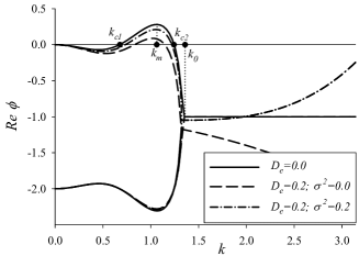
a)   b)

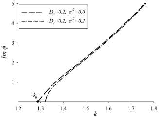
Figure 1: Real (a) and imaginary (b) parts of the phase $\phi(k)$ in the vicinity of the state $x_{0}=0$ at different values of the external flux parameters $D_{e}$ and $\sigma^{2}$. Other parameters are: $\theta=0.7$, $\tau_{D}=0.5$, $r_{c}=0.5$.

From Fig.1a it follows that in the simplest case $D_{e}=0$ (solid line) unstable modes are limited by the interval of the wave-numbers $k_{c1}\leq k\leq k_{c2}$. The deterministic external influence (dashed line) suppresses the instability progress, resulting to shrinking the domain of unstable modes. However, external fluctuations act in opposite manner to the deterministic part of the flux $\mathbf{J}_{e}$: the domain of unstable modes extends as $\sigma^{2}$ increases, and oscillating solutions emerge at large $k_{0}$ (see Fig.1b). Hence, we arrive at competing contributions of regular and random parts of the external flux. It should be noted that the wave-number responsible for the most unstable mode and, respectively, for the period of the formed structure depends on the temperature $\theta$ and the intensity $D_{e}$.

Let us study pattern selection processes considering dynamics of the structure function shown in Fig.2. It is seen that oscillations in time are observed at different values of the wave-number $k$. Such a behaviour is absolutely predictable according to the form of the dynamical equation for the structure function. More interesting is the wave behavior of $S$ versus the wave-number. The main peak in the dependence $S(k)$ is responsible for the main period of the structures, whereas other peaks reflects selection of patterns with small periods. These peaks decay with time growth that means selection of the one unstable mode $k\simeq k_{m}$ that gives the main contribution in the pattern formation processes. The same oscillations can be found in solutions of the equation for the average $\langle x\rangle$. From Fig.2a it is seen that during the system evolution the position of the main peak is shifted toward the most unstable mode $k\simeq k_{m}$; a width of the peak is reduced and it becomes higher. It means that the spatial patterns become well-defined with sharp interfaces.

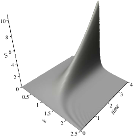
a)  b)

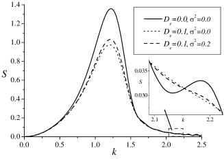
Figure 2: Evolution of the structure function at small times at $D_{e}=0.1$, $\sigma^{2}=0.2$ (a) and the structure function at $t=2$ for $\tau_{D}=1.0$, $r_{c}=1.0$, $\theta=0.7$.

From the dependencies $S(k)$ at a given $t$ it follows that the external flux has a crucial influence on the patterns selection processes. Here the regular part of the athermal flux ($D_{e}\neq 0$, $\sigma^{2}=0$) suppresses the pattern selecting, whereas its stochastic contribution ($\sigma^{2}\neq 0$) results in the amplification of the magnitude of the structure function peaks sustaining the pattern selection processes. Let us note that the competition of both regular and stochastic contributions of the external flux leads to the fact that the main peak in $S(k)$ dependence decreases at large $D_{e}$ and its width increases. It means that the corresponding patterns have more diffuse interfaces if additional (athermal) diffusion is introduced. However, the stochastic source of the flux $\mathbf{J}_{e}$ acts in the opposite manner. The main peak of the structure function is shifted toward large $k$ as the temperature $\theta$ decreases.

Let us consider stability of the state $x_{0}=\sqrt{1-\theta}$ at $\theta<1$. We are interesting in pattern selection processes in the vicinity of the minimum of the free energy density $f(x)$. From naive considerations one can say that the system should be stable in the vicinity of the free energy density minimum. Indeed, here the real part of the phase is negative, $\Re\phi(k)_{\pm}<0$ always (not presented here). The imaginary part can exist at $k>k_{0}$ (see Fig.3). Therefore, in the vicinity of $x_{0}=\sqrt{1-\theta}$ pattern selection is possible too. Here an increase in the noise intensity $\sigma^{2}$ results in a growth of the quantity $k_{0}$.

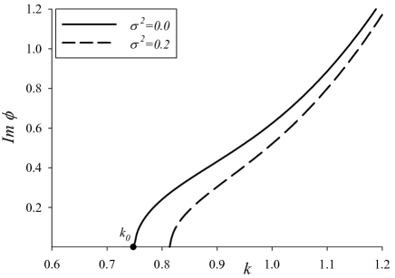
Figure 3: Imaginary part of the phase $\phi(k)$ of state $x_{0}=\sqrt{1-\theta}$ at $\tau_{D}=0.5$, $r_{c}=0.5$, $D_{e}=0.2$, $\theta=0.4$.

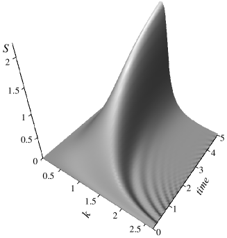
a) b)

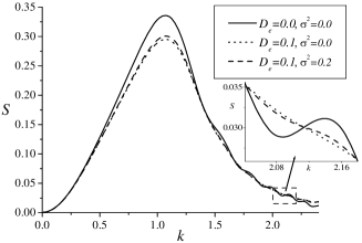
Figure 4: Evolution of the structure function (a) in the vicinity of the state $x_{0}=\sqrt{1-\theta}$ at $\sigma^{2}=0.2$, $D_{e}=0.1$ and the structure function at different $D_{e}$ and $\sigma^{2}$ at $t=2$ (b); $\theta=0.4$, $tau_{D}=1.0$, $r_{c}=0.65$.)

The structure function in the vicinity of the state $x_{0}=\sqrt{1-\theta}$ is shown in Fig.4 where oscillations versus time variable and wave-number is clearly seen. The position of the main peak of the structure function (see Fig.4a) does not change in time at large $t$ and its magnitude does not increase. It means that patterns are formed rapidly with sharp interfaces. From Fig.4b one can see that a height of the main peak is reduced as $D_{e}$ increases, the wave behaviour disappears. From another hand stochastic contribution of the flux $\mathbf{J}_{e}$ promotes an increase in the amplitude of the structure function oscillations and increase in the main peak height. Therefore, due to the stochastic external influence the spatial patterns become well-defined.

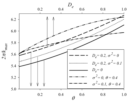
Figure 5: Dependencies of the period of patterns $2\pi/k_{max}$ versus temperature and coefficient $D_{e}$ and different $\sigma^{2}$ at $\tau_{D}=0.5$, $r_{c}=0.5$.

In Fig.5 we plot the dependence of the period of patterns $2\pi/k_{max}$ computed according to the wave-number $k_{max}$ related to the maximum of the structure function $S_{max}=S(k_{max})$ at large $t$ when the position of the main peak does not change. It is seen that the period of structures grows as temperature and the coefficient $D_{e}$ increases: thermal heating leads to formation of large patterns; and additional (athermal) diffusion results to the same effect due to the constant $D_{e}$ leads to renormalization of the effective temperature $\theta_{ef}=1-\theta+D_{e}$. At large $D_{e}$ period of patterns at the fixed $\theta$ increases, but the stochastic external source suppresses this growth .

4 Simulations

4.1 Discrete representation

In order to verify the previous predictions, one can perform numerical simulations of the discrete model (6) in a square two-dimensional lattice $N\times N$ of the cell size $\ell$. The partial differential equations (6) in the discrete space take the form

$$\begin{split}&\frac{{\rm d}x_{i}}{{\rm d}t}=-(\nabla_{R})_{ij}J_{j}+D_{e}\Delta_{ij}x_{j}+(\nabla_{R})_{ik}\zeta_{k}(\nabla_{L})_{kl}x_{l},\\ \tau_{D}&\frac{{\rm d}J_{i}}{{\rm d}t}=-J_{i}-M(\nabla_{L})_{ij}\frac{\partial F}{\partial x_{j}}+\xi_{i},\\ \tau_{\zeta}&\frac{{\rm d}\zeta_{i}}{{\rm d}t}=-(\delta_{ij}-r_{c}^{2}\Delta_{ij})\zeta_{j}+\tilde{\xi}_{i},\end{split}$$ (24)

where index $i$ labels cells, $i=1,\ldots,N^{2}$; the discrete left and right operators are introduced as follows

$$\begin{split}&(\nabla_{L})_{ij}=\frac{1}{\ell}(\delta_{i,j}-\delta_{i-1,j}),\quad(\nabla_{R})_{ij}=\frac{1}{\ell}(\delta_{i+1,j}-\delta_{i,j}),\\ &(\nabla_{L})_{ij}=-(\nabla_{R})_{ji},\quad(\nabla_{L})_{ij}(\nabla_{R})_{jl}=\Delta_{il}=\frac{1}{\ell^{2}}(\delta_{i,l+1}-2\delta_{i,l}+\delta_{i,l-1}).\end{split}$$ (25)

For the stochastic sources the discrete correlator is of the form $\langle\xi_{i}(t)\xi_{j}(t)\rangle=2\ell^{2}\sigma^{2}\delta_{ij}\delta(t-t^{\prime})$. In the limit $\tau_{\zeta}\ll 1$ one has quasi-white noise with $\langle\tilde{\xi}_{i}(t)\rangle=0$, $\langle\tilde{\xi}_{i}(t)\tilde{\xi}_{j}(t^{\prime})\rangle\simeq\delta_{ij}\delta(t-t^{\prime})$. Under these conditions we arrive at the stochastic process with properties given by Eq.(3).

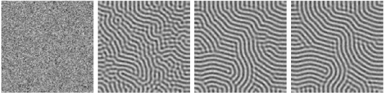
Figure 6: Evolution of patterns at $\theta=0.3$, $D_{e}=0.5$, $\sigma^{2}=1.0$, $\tau_{D}=0.5$, $r_{c}=1.0$. Snapshots are taken at $t=0$, 50, 500, 1000.

Simulations are provided with the time step $\delta t=10^{-3}$ on the square lattice of the size $128\times 128$ with $\ell=1$. Typical evolution of the system is shown in Fig.6 with initial conditions $\langle x(\mathbf{r},t=0)\rangle=0$, $\langle(\delta x)^{2}\rangle=0.3$. It is seen that linear patterns are formed that corresponds to the standard analysis of the pattern formation in deterministic systems with such initial conditions [18].

4.2 Analysis of the wave behavior

To prove the wave behavior of the first statistical moment and the structure function we analyze the dynamics of two first statistical moments. While the considered system obeys a mass conservation law ($\int{\rm d}{\mathbf{r}}x(\mathbf{r},t)=const$, where $const=0$), in our computer simulations we calculate averages that correspond to positive and negative values of the stochastic field $x$, i.e. $\langle x\rangle_{+}=\langle N^{-2}\sum_{i}x_{i}^{>}\rangle$, where $x_{i}^{>}$ relates to $x_{i}>0$, and $\langle x\rangle_{-}=\langle N^{-2}\sum_{i}x_{i}^{<}\rangle$, where $x_{i}^{<}$ relates to $x_{i}<0$, $\langle\ldots\rangle$ means average over experiments. If the ordering processes realize, then the quantities $\langle x\rangle_{+}$, $\langle x\rangle_{-}$ should increase during the system evolution satisfying the conservation law $\langle x\rangle\equiv\langle x\rangle_{+}+\langle x\rangle_{-}=0$. Another criterion for an existence of an ordered state is growth of the averaged second moment $J=\langle N^{-2}\sum_{i}x_{i}^{2}\rangle$ which in pattern selection discussion is known as a convective heat; it plays a role of an order parameter in pattern-forming transitions theory [40]. An alternative definition is $J(t)=\sum_{k}S(k,t)$, where $S(k,t)$ is a spherically averaged structure function. Hence $J(t)$ gives the square under the function $S(k,t)$. Therefore, possible oscillations in $J(t)$ should manifest the wave behavior of the structure function versus time. To prove the existence of pattern selection processes we analyze the spherically averaged structure function calculated according to standard definition $S(k,t)=({N_{k}})^{-1}\sum_{k\leq\mathbf{k}\leq k+\Delta k}S_{\mathbf{k}}(t)$.

Results of our computer simulations indicate that the constituents of the total average $\langle x(t)\rangle_{\pm}$ and the order parameter $J(t)$ increase manifesting oscillations (see Fig.7a). Moreover, oscillations of $\langle x\rangle_{+}$ and $\langle x\rangle_{-}$ are realized in an antiphase manner that satisfies the conservation law. An increase of the order parameter $J(t)$ means the ordering of the system; the corresponding oscillations reflects the time oscillations of the structure function. In Fig.7b we plot the spherically averaged structure function for nonlinear system. It is seen that the wave behavior versus $k$ is realized. With an increase in the time $t$ additional peaks disappear (not presented here). We plot the dependence at $\tau_{D}=1$. At $\tau_{D}<1$ these peaks are not well pronounced but exist. Heights of such peaks can be increased setting $\tau_{D}>1$. In our case we consider a limit $\tau_{D}\leq 1$ assuming that time scales for the field $x$ and the flux $\mathbf{J}_{D}$ can be commensurable.

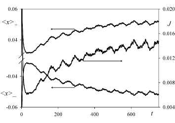
a) b)

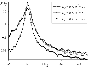
Figure 7: Evolution of averages $\langle x\rangle_{+}$, $\langle x\rangle_{-}$ and the order parameter $J=\langle x^{2}\rangle$ (a) at $\tau_{D}=0.5$, $r_{c}=1.0$, $\theta=0.5$, $D_{e}=0.5$, $\sigma^{2}=1.0$ and the spherically averaged structure function $S(k)$ (b) at $t=1000$, $\tau_{D}=1.0$, $r_{c}=1.0$, $\theta=0.2$, $D_{e}=0.1$, $\sigma^{2}=0.2$

4.3 Noise-induced pattern-forming transitions

As was shown above the interactions provided by the Swift-Hohenberg coupling operator lead to nonequilibrium pattern-forming transitions. In this subsection we aim to study these transitions by means of standard technique employed in the equilibrium phase transitions analysis. In the nonequilibrium case the relative order parameter is the steady state quantity $\eta\equiv\lim_{t\to\infty}\overline{\langle{J}\rangle}$, where $\overline{\ldots}$ means average over large time interval. We can use an additional criterion $m_{+}\equiv\lim_{t\to\infty}\overline{\langle x(t)\rangle_{+}}$ to characterize the ordered state. The extensive related fluctuations are given by the quantity $\chi=N^{-2}\overline{(\langle J^{2}\rangle-\langle J\rangle^{2})/\langle J\rangle^{2}}$ playing a role of the generalized susceptibility. From these definitions it follows that in the disordered (homogeneous) state one has $\eta=m_{+}=0$, in the ordered state the order parameter takes nontrivial values ($\eta\neq 0$). In the vicinity of the critical point (for example $\theta\simeq\tilde{\theta}_{c}$) fluctuations grow and the susceptibility $\chi$ increases.

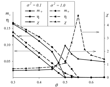
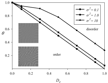
Figure 8: Plots of the steady state order parameter $\eta$, the average $m_{+}$ and the susceptibility $\chi$ (a) at $D_{e}=0.5$ and phase diagram for nonequilibrium pattern-forming transitions (b). Other parameters are: $\tau_{D}=0.5$, $r_{c}=1.0$.

In Fig.8а we plot steady state order parameter $\eta$ and the average $m_{+}$ versus temperature and the parameter $D_{e}$ at different values of the external noise intensity $\sigma^{2}$. It is seen that as the temperature and ballistic mixing intensity $D_{e}$ grow the order parameter and the average $m_{+}$ decreases. In the vicinity of the critical point $\theta\simeq\tilde{\theta}_{c}$ the generalized susceptibility shows a well defined maximum at the same location where the order parameter departs from zero. It clearly seen that external fluctuations results in renormalization of the critical value for the control parameter $\varepsilon$. One can find that the critical value for the noise-induced patterning tends to its mean filed value $\theta_{c}=1$ as the noise intensity increases at fixed $D_{e}$ that decreases $\tilde{\theta}_{c}$. To illustrate the noise-induced shift of the critical point we compute the phase diagram shown in Fig.8b. It follows that at fixed noise intensity $\sigma^{2}$ the critical value $\tilde{\theta}_{c}$ decreases as the ballistic mixing intensity $D_{e}$ grows. One can see that if $\sigma^{2}$ increases, then instability of the disordered state emerge at elevated temperatures. This conclusion is in agreement with the prediction made above from the liner stability analysis. Moreover, it should be noted that in the domain in the vicinity of $\tilde{\theta}_{c}$ where the fluctuations are large the spatial patterns have diffuse interfaces, whereas at out off critical temperatures $\tilde{\theta}_{c}$ spatial patterns are well-defined (see insertions in the phase diagram).

5 Conclusions

We have studied pattern selection processes in periodic stochastic systems with the hyperbolic transport. Considering the system with thermally sustained flux and flux of athermal mixing we discuss properties of pattern formation, selection and nonequilibrium pattern-forming transitions. The dynamics is studied in terms of both the first statistical moment and the structure function. Analytical results related to the linear stability analysis are compared with computer simulations. We have found that external athermal flux having both regular and stochastic components influences crucially on pattern selection processes. It was shown that regular part of the external flux suppresses such processes, whereas it stochastic constituent promotes the pattern selection. Considering pattern-forming transitions we have shown that external influence shifts the critical point of the transition where the regular and random components of the external flux act in competing manner.

References

- [1] G.Ahlers, D.S.Cannell, V.Steinberg, Phys.Rev.Lett. 54, 1373 (1985)
- [2] C.W.Meyer, G.Ahlers, D.S.Cannell, Phys.Rev.A. 44, 2514 (1991)
- [3] S.W.Morris, E.Bodenshaltz, D.S.Cannell, A.Ahlers, Phys.Rev.Lett. 71, 2026 (1993)
- [4] A. S. Mikhailov and K. Showalter, Phys.Rep. 425, 79 (2006)
- [5] H.Katsuragi, Eur.Phys.Lett. 73, 793, (2006)
- [6] F.Sagues, J.M.Sancho, J.Garcia-Ojalvo. Rev.Mod.Phys., 79, 829 (2007)
- [7] B.Lindner, J.GArcia-Ojalvo, A.Neiman, L.Shimansky-Geier, Phys.Rep. 392, 321 (2004)
- [8] G.Stegemann, A.G.Balanov, E.Schöll, Phys.Rev.E. 71, 016221 (2005)
- [9] Sergio E. Mangioni, Horacio S.Wio. Phys.Rev.E 71, 056203 (2005).
- [10] D.Kharchenko, S.V.Kokhan, A.V.Dvornichenko, Physica D 238, 2251 (2009)
- [11] D.Kharchenko, S.V.Kokhan, A.V.Dvornichenko, Metallofiz. Noveishie Tekhnol. 31, 1, 23 (2009)
- [12] V.Kharchenko, Physica A 388, 268 (2009)
- [13] Sergio E. Mangioni, Physica A 389, 1799 (2010)
- [14] Raul A. Enrique, Pascal Bellon, Phys.Rev.B 63, 134111 (2001)
- [15] Jia Ye, Pascal Bellon, Phys.Rev.B 70, 094104 (2004)
- [16] Jie Lian, Wei Zhou, Q.M.Wei et al. Appl.Phys.Lett. 88, 093112 (2006)
- [17] R.Kree, T.Yasseri, A.K.Hartmann, Nucl.Ins.Meth.B 267, 1407 (2009)
- [18] K.R.Elder, M.katakowski, M.Haataja, M.Grant, Phys.Rev.Lett. 88, 245701 (2002)
- [19] A.Jaatinen, C.V.Achim, K.R.Elder et al. Phys.Rev.E 80, 031602 (2009)
- [20] J.Berry, M.Garnt, K.R.Elder, Phys.Rev.E 73, 031609 (2006)
- [21] J.Swift, P.C.Hohenberg, Phys.Rev.A 15, 319 (1977)
- [22] P.Stefanovich, M.Haataja, N.Provatas, Phys.Rev.Lett. 96, 225504 (2006)
- [23] K.R.Elder, J.Vinals, M.Grant, Phys.Rev.Lett. 68, 3024 (1992)
- [24] J.Garcia-Ojalvo, A.Hernandez-Machado, J.M.Sancho, Phys.Rev.Lett. 71, 1542 (1993)
- [25] J.Garcia-Ojalvo, J.M.Sancho, Int.J.Bif.Chaos 4, 1337 (1994)
- [26] J.Garcia-Ojalvo, J.M.Sancho, Phys.Rev.E 53, 5680 (1996)
- [27] J.M.R.Parrondo, C. Van der Broeck, J.Buceta et al., Physica A 224, 153 (1996)
- [28] A.A.Zaikin, L.Shimansky-Geier, Phys.Rev.E 58, 4355 (1998)
- [29] K.Wood, J.Buceta, K.Lindenberg, Phys.Rev.E 73, 022101 (2006)
- [30] D.Jou, J.Casas Vazquez, G.Lebon, Extended Irreversible Thermodynamics, 3rd edition (Springer-Verlag, Berlin, 2001)
- [31] P.Galenko, D.danilov, V.Lebedev, Phys.Rev.E 79, 051110 (2009)
- [32] D.O.Kharchenko, A.V.Dvornichenko, Physica A 387, 5342 (2008).
- [33] A.A. Ponomarov, V.I. Miroshnichenko, A.G. Ponomarev, Nucl.Ins.Meth.B 267, 2041 (2009)
- [34] V.I.Dubinko, A.V.Tur, V.V.Yanovsky, Rad.Eff. 112, 233 (1990)
- [35] K.R.Elder, Martin Grant. Phys.Rev.E 70, 051605 (2004).
- [36] K.R.Elder, Nikolas Provatas, Joel Berry, Peter Stefanovich, Martin Grant, Phys.Rev.B 75, 064107 (2007)
- [37] Joel Berry, K.R.Elder, Martin Grant, Phys.Rev.E 77, 061506 (2008)
- [38] N. Lecoq, H. Zapolsky, P. Galenko, European Physical Journal ST 177, 165 (2009)
- [39] E.A. Novikov, Zh. Eksp. Teor. Fiz. 47, 1919 (1964). English Translation, Sov. Phys. JETP 20, 1290 (1965)
- [40] J. Garcia–Ojalvo, J.M. Sancho, Noise in Spatially Extended Systems (Springer, New York, 1999)