Cyclotron harmonics in opacities of isolated neutron star atmospheres

Some X-ray dim isolated neutron stars (XDINS) and central compact objects in supernova remnants (CCO) contain absorption features in their thermal soft X-ray spectra. It has been hypothesized that this absorption may relate to periodic peaks in free-free absorption opacities, caused by either Landau quantization of electron motion in magnetic fields $B\lesssim 10^{11}$ G or analogous quantization of ion motion in magnetic fields $B>10^{13}$ G. Here, I review the physics behind cyclotron quantum harmonics in free-free photoabsorption, discuss different approximations for their calculation, and explain why the ion cyclotron harmonics (beyond the fundamental) cannot be observed.

1 Introduction

Thermal radiation from neutron stars can provide important information about their physical properties. Among neutron stars with thermal-like radiation spectra (see, e.g., reviews by Kaspi et al. 2006 and Zavlin 2009), there are two classes of objects of particular interest: central compact objects (CCOs; see, e.g., de Luca 2008) in supernova remnants and X-ray dim isolated neutron stars (XDINSs, or the Magnificent Seven; see, e.g., review by Turolla 2009).

The CCOs are young, radio-quiet isolated neutron stars with relatively weak magnetic fields $B\sim(10^{10}-10^{11})$ G (e.g., Halpern & Gotthelf 2010 and references therein). The XDINSs are older and are believed to have much stronger fields $B\gtrsim(10^{12}-10^{13})$ G (Haberl 2007; van Kerkwijk & Kaplan 2007; Turolla 2009). For some CCOs and XDINSs, there are estimates of $B$, and in some cases only upper limits to $B$ are available.

In the past decade, broad absorption lines have been detected in the thermal spectra of several isolated neutron stars (see, e.g., van Kerkwijk 2004; Haberl 2007; van Kerkwijk & Kaplan 2007, and references therein). In all but one case, the energies $E_{\mathrm{a}}^{\infty}$ of the absorption are centered on the range 0.2–0.7 keV and the effective black-body temperatures are $T_{\mathrm{eff,bb}}^{\infty}\approx 0.1$ keV. Here and hereafter, the Boltzmann constant is suppressed, and the superscript “$\infty$” indicates a redshifted value. In particular, it has been found that: (i) the spectrum of RX J1605.3+3249 with $T_{\mathrm{eff,bb}}^{\infty}\approx 96$ eV has a broad absorption at $E_{\mathrm{a}}^{\infty}\approx 0.4$–0.5 keV and a possible second absorption at 0.55 keV (van Kerkwijk et al. 2004; van Kerkwijk 2004); (ii) RX J0720.4-3125 exhibits an absorption feature at $E_{\mathrm{a}}^{\infty}\approx 0.27$ keV (Haberl et al. 2004) and a possible second absorption at 0.57 keV (Hambaryan et al. 2009), while the effective black-body temperature varies over years across the range $T_{\mathrm{eff,bb}}^{\infty}\approx 86$–95 eV (Hohle et al. 2009); (iii) the spectrum of RBS1223 (RX J$1308.6+2127$) was reproduced by a model with $T_{\mathrm{eff,bb}}^{\infty}\approx 102\pm 2$ eV and two absorption lines at $E_{\mathrm{a}}^{\infty}\sim 0.3$ keV and $E_{\mathrm{a}}^{\infty}\sim 0.6$ keV (Schwope et al. 2007); and (iv) the spectrum of RBS1774 (1RXS J$214303.7+065419$) with $T_{\mathrm{eff,bb}}^{\infty}\approx 102$ eV shows indications of a line at $E_{\mathrm{a}}^{\infty}\approx 0.3$–0.4 keV and an absorption edge at $0.73$–0.75 keV (Cropper et al. 2007; Kaplan & van Kerkwijk 2009; Schwope et al. 2009). The first discovered isolated neutron star with absorption lines, CCO 1E 1207.4-5209, has two absorption features centered on $E_{\mathrm{a}}^{\infty}\approx 0.7$ keV and 1.4 keV (Sanwal et al. 2002) and an effective black-body temperature (which may be nonuniform) of $T_{\mathrm{eff,bb}}^{\infty}\sim 0.16$–0.32 keV (Zavlin et al. 1998; de Luca et al. 2004). For this object, two more harmonically spaced absorption features (at $E_{\mathrm{a}}^{\infty}\approx 2.1$ keV and 2.8 keV) were tentatively detected (Bignami et al. 2003; de Luca et al. 2004), but were later shown to be statistically insignificant (Mori et al. 2005). We note that realistic values of the effective temperature $T_{\mathrm{eff}}^{\infty}$, obtained using atmosphere models, can differ from $T_{\mathrm{eff,bb}}^{\infty}$ by a factor $\lesssim 2$–3 (see, e.g., Zavlin 2009, and references therein).

Many authors (e.g., Sanwal et al. 2002; Bignami et al. 2003; de Luca et al. 2004) have considered the theoretical possibility that the absorption lines in the thermal spectra of the CCOs and XDINSs may be produced by cyclotron harmonics, formed because of quantum transitions between different Landau levels of charged particles in strong magnetic fields. Zane et al. (2001) discussed this possibility prior to the observational discovery of these absorption features. The fundamental cyclotron energy equals

$$\hbar\omega_{\mathrm{c}}=\hbar{eB/mc}=11.577\leavevmode\nobreak\ B_{12}\textrm{ keV}$$ (1)

for the electrons and $\hbar\Omega_{\mathrm{c}}=\hbar{ZeB/Mc}=6.35\,(Z/A)B_{12}$ eV for the ions, where $m$ and $M$ are the electron and ion masses, respectively, $Z$ and $A$ are the ion charge and mass numbers, and $B_{12}\equiv B/10^{12}$ G. In the following, we consider protons, whose cyclotron energy is

$$\hbar\Omega_{\mathrm{c}}=\hbar eB/Mc=6.305\,B_{12}\textrm{ eV}.$$ (2)

Beginning with the pioneering work of Gnedin & Syunyaev (1974), numerous papers have been devoted to the physics and modeling of cyclotron lines in X-ray spectra of accreting neutron stars (e.g., Daugherty & Ventura 1977; Pavlov et al. 1980; Wang et al. 1993; Araya & Harding 1999; Araya-Góchez & Harding 2000; Nishimura 2005, 2008). These emission lines have been observed in many works following their discovery by Trümper et al. (1978). Cyclotron harmonics have been found in spectra of several X-ray pulsars in binaries (e.g., Rodes-Roca et al. 2009; Enoto et al. 2008; Pottschmidt et al. 2004, and references therein), and up to four harmonics were registered for one of them (Santangelo et al. 1999).

In the photospheres of isolated neutron stars, unlike X-ray binaries, the typical energies of charged particles are nonrelativistic. In this case, first-order cyclotron transitions of free charged particles are dipole-allowed only between neighboring equidistant Landau levels and form a single cyclotron resonance with no harmonics. Special relativity and non-dipole corrections at the energies of interest can be estimated to be $\mathrm{max}(T_{\mathrm{eff}},E_{\mathrm{a}})/mc^{2}\sim 10^{-3}$ for the electrons and $\mathrm{max}(T_{\mathrm{eff}},E_{\mathrm{a}})/Mc^{2}<10^{-6}$ for the protons.

Beyond the first order in interactions, transitions between distant Landau states are also allowed in the nonrelativistic theory. They are, in particular, caused by Coulomb interactions between plasma particles. Thus cyclotron harmonics appear in free-free (bremsstrahlung) cross-sections. To obtain $E_{\mathrm{a}}\sim 0.1$–1 keV, one may assume either the electron cyclotron harmonics at $B\sim 10^{10}$–$10^{11}$ G, according to Eq. (1), or proton cyclotron harmonics at $B\sim 10^{13}$–$10^{14}$ G, according to Eq. (2).

Pavlov & Shibanov (1978) presented the calculations of spectra for isolated neutron stars with prominent electron cyclotron harmonics due to the free-free absorption in the atmosphere. Suleimanov et al. (2010b) performed a similar atmosphere modeling and concluded, in agreement with Zane et al. (2001), that electron cyclotron harmonics could be observed in CCO spectra. Proton cyclotron harmonics cannot be calculated based on the assumption of classical proton motion, used by these authors.

In this paper, I review the physics of free-free photoabsorption in strong magnetic fields, discuss restrictions on different published approximations for free-free opacities, and present numerical results that demonstrate the relative strengths of the electron and proton cyclotron resonances under the conditions characteristic of the atmospheres of isolated neutron stars with strong magnetic fields. This gives a graphic explanation of the smallness of the ion cyclotron harmonics. I also demonstrate that the contribution of bound-bound and bound-free transitions to the opacities of neutron stars with $B>10^{13}$ G is much larger than that of the proton cyclotron harmonics.

In Sect. 2, quantum mechanical integrals of motion and wave functions of a charged particle in a magnetic field are recalled for subsequent use. Section 3 is devoted to the properties of an electron-proton system in a magnetic field that is quantizing for both particles: general equations for calculation of wave functions are given, and the Born approximation is considered in detail. In the same order, general expressions and Born approximation are considered in Sect. 4 for photoabsorption matrix elements and cross-sections. Section 5 gives numerical examples of cyclotron harmonics in free-free photoabsorption with discussion and comparison of various approximations. Consequences for the CCOs and XDINSs are discussed in Sect. 6, and Sect. 7 presents our summary.

2 Charged particles in a magnetic field

Since special relativity effects are of minor importance in the atmospheres of isolated neutron stars, we use nonrelativistic quantum mechanics.

We assume that the magnetic field vector $\@vec{B}$ is along the $z$ axis and consider its vector potential the cylindrical gauge to be

$$\@vec{A}(\@vec{r})=\frac{1}{2}\,\@vec{B}\times(\@vec{r}-\@vec{r}_{A})$$ (3)

with an arbitrary center $\@vec{r}_{A}$ in the $xy$ plane.

We recall the description of a charged particle in a uniform magnetic field (e.g., Johnson & Lippmann 1949; Landau & Lifshitz 1976; Johnson et al. 1983). The Hamiltonian equals the kinetic energy operator

$$H^{(1)}=\frac{m\dot{\@vec{r}}^{2}}{2}=H_{\perp}^{(1)}+\frac{p_{z}^{2}}{2m},\qquad H_{\perp}^{(1)}=\frac{m\dot{\@vec{r}}_{\perp}^{2}}{2},$$ (4)

where $m$ is the mass,

$$m\dot{\@vec{r}}=\@vec{p}-(Q/c)\,\@vec{A}(\@vec{r})$$ (5)

is the kinetic momentum, $Q$ is the charge, and $\@vec{p}$ is the canonical momentum conjugate to $\@vec{r}$. In Eq. (4) and hereafter, “$\perp$” denotes the “transverse” part, related to the motion in the $xy$ plane.

A classical particle moves along a spiral around the normal to the $xy$ plane at the guiding center $\@vec{r}_{c}$. In quantum mechanics, $\@vec{r}_{c}$ is an operator, related to the pseudomomentum operator

$$\hbar\@vec{k}=m\dot{\@vec{r}}+(Q/c)\,\@vec{B}\times\@vec{r},$$ (6)

where $\@vec{r}_{c}=(c/QB^{2})\,\hbar\@vec{k}\times\@vec{B}$. Its cartesian coordinates $(x_{c},y_{c})$ commute with $H_{\perp}^{(1)}$, but do not commute with each other: $[x_{c},y_{c}]=-\mathrm{i}\hbar c/QB$. Another important integral of motion is the $z$-projection of the angular momentum $\ell_{z}=(QB/c)\,(r_{c}^{2}/2-H_{\perp}^{(1)}/m\omega_{\mathrm{c}}^{2})$, where $\omega_{\mathrm{c}}=|Q|B/mc$ is the cyclotron frequency.

The eigenvalues of $H_{\perp}^{(1)}$ are given by $E^{\perp}_{n}=(n+\frac{1}{2})\hbar\omega_{\mathrm{c}}$, where $n=0,1,2,\ldots$ is the Landau quantum number. The simultaneous eigenvalues of $\ell_{z}$ are ($\mathrm{sign}\,Q)\,\hbar s$ with integer $s\geq-n$, and eigenvalues of the squared guiding center $r_{c}^{2}$ equal to $a_{\mathrm{m}}^{2}(2s+2n+1)$, where $a_{\mathrm{m}}=(\hbar c/|Q|B)^{1/2}$ is the so-called magnetic length.

In general, $H_{\perp}^{(1)}$ should be supplemented by $(-\@vec{B}\cdot\hat{\@vec{\mu}})$, where $\hat{\@vec{\mu}}=g_{\mathrm{mag}}\,(e/2mc)\,\hat{\@vec{S}}$ is the intrinsic magnetic moment of the particle, $\hat{\@vec{S}}$ is the spin operator, and $g_{\mathrm{mag}}$ is the spin $g$-factor ($g_{\mathrm{mag}}=-2.0023$ and $5.5857$ for the electron and the proton, respectively). In most applications, one can choose the representation where the electron and proton spins have definite $z$-projections $\pm\hbar/2$ and set the electron $g$-factor to $-2$, thus regarding the excited electron Landau levels as double degenerate.

The form of a wave function depends on a choice of the gauge for $\@vec{A}(\@vec{r})$. We consider the cylindrical gauge given by Eq. (3) centered on the coordinate origin ($\@vec{r}_{A}=\@vec{0}$). The eigenfunctions of $H^{(1)}$ and $\ell_{z}$ in the coordinate representation are

$$\Psi_{n,s,k_{z}}(\@vec{r})=\frac{\mathrm{e}^{\mathrm{i}k_{z}z}}{L_{z}^{1/2}}\times\left\{\begin{array}[]{ll}\Phi_{n,s}(\@vec{r}_{\perp}),&\mbox{if $Q<0$}\\ \Phi^{\ast}_{n,s}(\@vec{r}_{\perp}),&\mbox{if $Q>0$}\end{array}\right.,$$ (7)

where $k_{z}=p_{z}/\hbar$ is the particle wave number along the field, $L_{z}$ is the normalization length, $\@vec{r}_{\perp}=(x,y)=(r_{\perp}\cos\phi,r_{\perp}\sin\phi)$,

$$\Phi_{n,s}(\@vec{r}_{\perp})=\frac{\mathrm{e}^{-\mathrm{i}s\phi}}{\sqrt{2\pi}\,a_{\mathrm{m}}}\,I_{n+s,n}(r_{\perp}^{2}/2a_{\mathrm{m}}^{2})$$ (8)

is Landau function, the asterisk denoting a complex conjugate, and $I_{n^{\prime}n}(u)$ is a Laguerre function (e.g., Sokolov & Ternov 1986).

We define cyclic components of any vector $\@vec{a}$ as $a_{\pm 1}=(a_{x}\pm\mathrm{i}a_{y})/\sqrt{2}$ and $a_{0}=a_{z}$. The transverse cyclic components of the kinetic momentum operator given by Eq. (5) transform one Landau state $|n,s\rangle_{\perp}$, characterized by $\Phi_{ns}^{(\ast)}(\@vec{r}_{\perp})$, into another Landau state

$$m\dot{\@vec{r}}_{\alpha}\,|n,s\rangle_{\perp}=\frac{\hbar\tilde{\alpha}}{\mathrm{i}a_{\mathrm{m}}}\sqrt{n+1/2+\tilde{\alpha}/2}\,|n+\tilde{\alpha},s-\tilde{\alpha}\rangle_{\perp},$$ (9)

where $\alpha=\pm 1$, $\tilde{\alpha}=\alpha$ if $Q<0$, and $\tilde{\alpha}=-\alpha$ if $Q>0$.

3 Electron-proton system in a magnetic field

The Hamiltonian of the electron-proton pair (i.e., of H atom) is

$$H=H_{\mathrm{e}}^{(1)}+H_{\mathrm{p}}^{(1)}-\frac{e^{2}}{r_{\mathrm{ep}}},$$ (10)

where $\@vec{r}_{\mathrm{ep}}=\@vec{r}_{\mathrm{e}}-\@vec{r}_{\mathrm{p}}$. The kinetic part can be written as

$$H_{\mathrm{e}}^{(1)}+H_{\mathrm{p}}^{(1)}=\frac{M\dot{\@vec{r}}_{\mathrm{p}}^{2}}{2}+\frac{m\dot{\@vec{r}}_{\mathrm{e}}^{2}}{2}=\frac{m_{\mathrm{H}}\dot{\@vec{R}}^{2}}{2}+\frac{m_{\ast}\dot{\@vec{r}}^{2}}{2},$$ (11)

where $m$ and $M$ are the electron and ion masses, $\@vec{R}=(M/m_{\mathrm{H}})\,\@vec{r}_{\mathrm{p}}+(m/m_{\mathrm{H}})\,\@vec{r}_{\mathrm{e}}$ is the center of mass, $m_{\mathrm{H}}=m+M$ is the total mass, and $m_{\ast}=mM/m_{\mathrm{H}}$ is the reduced mass.

Since the electron and the proton have opposite charges, their orbiting in the transverse plane is accompanied by a drift across the magnetic field lines with velocity $\@vec{v}_{\mathrm{drift}}$ depending on the distance between their guiding centers or equivalently on the total pseudomomentum $\@vec{K}$

$$\@vec{r}_{c}=\@vec{r}_{c,e}-\@vec{r}_{c,p}=\frac{c}{eB^{2}}\,\@vec{B}\times\@vec{K},\quad\@vec{K}=\@vec{P}-\frac{e}{2c}\,\@vec{B}\times\@vec{r}_{\mathrm{ep}},$$ (12)

where $\@vec{P}$ is the canonical momentum conjugate to $\@vec{R}$.

In quantum mechanics, it is not only true that the pseudomomentum operator $\@vec{K}=\hbar\@vec{k}_{\mathrm{e}}+\hbar\@vec{k}_{\mathrm{p}}$ commutes with $H$, but also that its cartesian components $(K_{x},K_{y},K_{z})$ commute with each other. Therefore, all components of $\@vec{r}_{c}$ can be determined simultaneously. Coordinate eigenfunctions of the pseudomomentum operator with eigenvectors $\@vec{K}$ are given by (Gor’kov & Dzyaloshinskii 1968)

$$\Psi(\@vec{r}_{\mathrm{e}},\@vec{r}_{\mathrm{p}})=\exp\left[\frac{\mathrm{i}}{\hbar}\left(\@vec{K}+\frac{e}{c}\,\@vec{B}\times\@vec{r}_{\mathrm{ep}}\right)\cdot\@vec{R}\right]\,\psi_{\@vec{K}}(\@vec{r}_{\mathrm{ep}}).$$ (13)

From the general Schrödinger equation $H\Psi=E\Psi$, one can derive an equation for $\psi_{\@vec{K}}(\@vec{r}_{\mathrm{ep}})$, which has the form

$$H_{\mathrm{rel}}\,\psi_{\@vec{K}}=E\,\psi_{\@vec{K}},$$ (14)

where the effective Hamiltonian $H_{\mathrm{rel}}$ depends on $\@vec{K}$.

3.1 Exact solution

Solutions of Eq. (14) for arbitrary $\@vec{K}$ in strong magnetic fields in the cylindrical gauge represented by Eq. (3) were obtained by Vincke et al. (1992) and Potekhin (1994) for bound states, and by Potekhin & Pavlov (1997) for continuum states of the electron-proton system. Potekhin (1994) used the variable $\@vec{r}=\@vec{r}_{\mathrm{ep}}-\@vec{r}_{B}$ as an independent argument of the wave function and found that the most convenient parametrization in Eq. (3) is $\@vec{r}_{A}=[(M-m)/m_{\mathrm{H}}]\,\@vec{r}_{B}.$ Then

$$H_{\mathrm{rel}}=\frac{P_{z}^{2}}{2m_{\mathrm{H}}}+\frac{p_{z}^{2}}{2m_{\ast}}+H_{\perp}-\frac{e^{2}}{|\@vec{r}+\@vec{r}_{B}|},$$ (15)

where

$$H_{\perp}=\frac{{\pi}_{\perp}^{2}}{2m_{\ast}}-\frac{e}{Mc}\,\@vec{B}\cdot(\@vec{r}\times\@vec{p})+H_{K}$$ (16)

is the Hamiltonian of the harmonic motion in the $xy$ plane, $\@vec{p}$ is the momentum conjugate to $\@vec{r}$,

$$\@vec{\pi} = \@vec{p}+\frac{e}{2c}\,\@vec{B}\times\@vec{r},$$ (17)

$$H_{K} = \frac{K_{B}^{2}}{2m_{\mathrm{H}}}+\frac{e}{m_{\mathrm{H}}c}\,\@vec{K}_{B}\cdot(\@vec{B}\times\@vec{r}),\quad\mbox{and}\quad\@vec{K}_{B}=\@vec{K}+\frac{e}{c}\,\@vec{B}\times\@vec{r}_{B}.$$ (18)

We note that $H_{K}=0$ when $\@vec{r}_{B}=\@vec{r}_{c}$.

The first term in Eq. (15) is the total kinetic energy along $z$, uncoupled from the relative electron-proton motion, therefore we set $P_{z}=0$ without loss of generality.

The eigenvalues of $H_{\perp}$ equal $E^{\perp}_{ns}=E^{\perp}_{n}+E^{\perp}_{N},$ where $n\geq 0$ and $N=n+s\geq 0$ are the electron and proton Landau numbers, respectively, and $\hbar s$ are eigenvalues of the relative angular momentum projection operator ($\ell_{z,p}-\ell_{z,e}$).

We construct numerical solutions of Eq. (14) in the energy representation for $\@vec{r}_{B}=\eta\,\@vec{r}_{c}$ ($\eta\in[0,1]$) in the form

$$\psi_{\kappa}^{(\eta)}(\@vec{r})=\sum_{n^{\prime}s^{\prime}}\Phi_{n^{\prime}s^{\prime}}(\@vec{r}_{\perp})\,g^{(\eta)}_{n^{\prime},s^{\prime};\,\kappa}(z),$$ (19)

where $\kappa$ is the composite quantum number enumerating quantum states. One retains in Eq. (19) as many terms ($n=0,1,2,\ldots,n_{\mathrm{max}}$; $s=-n,-n+1,-n+2,\ldots,s_{\mathrm{max}}$) as needed to reach the desired accuracy. We choose a principal (“leading”) term $(n,s)$ and define “longitudinal” energy of the state $|\kappa\rangle$ as $E^{\|}_{\kappa}=E_{\kappa}-E^{\perp}_{ns}.$ The functions $g^{(\eta)}_{n^{\prime},s^{\prime};\,\kappa}(z)$ are computed from

$$\Bigg{(}-\frac{\hbar^{2}}{2m_{\ast}}\,\frac{\mathrm{d}^{2}}{\mathrm{d}z^{2}}+V_{n^{\prime\prime}s^{\prime\prime},n^{\prime\prime}s^{\prime\prime}}(r_{B},z)+\langle n^{\prime\prime}s^{\prime\prime}\,|\,H_{K}\,|\,n^{\prime\prime}s^{\prime\prime}\rangle_{\perp}$$

$$\quad+E^{\perp}_{n^{\prime\prime}s^{\prime\prime}}-E^{\perp}_{ns}-E^{\|}_{\kappa}\,\Bigg{)}\,g_{n^{\prime\prime}s^{\prime\prime};\,\kappa}(z)=$$

$$\qquad-{\sum}^{\prime}\big{(}V_{n^{\prime\prime}s^{\prime\prime},n^{\prime}s^{\prime}}(r_{B},z)+\langle n^{\prime\prime}s^{\prime\prime}\,|H_{K}|\,n^{\prime}s^{\prime}\rangle_{\perp}\big{)}\,g_{n^{\prime}s^{\prime};\,\kappa}(z),$$ (20)

where $n^{\prime\prime}=0,1,2,\ldots,n_{\mathrm{max}}$, $s^{\prime\prime}=-n^{\prime\prime},-n^{\prime\prime}+1,-n^{\prime\prime}+2,\ldots,s_{\mathrm{max}},$ $\Sigma^{\prime}$ denotes the sum over all pairs $(n^{\prime},s^{\prime})$ except $(n^{\prime\prime},s^{\prime\prime})$, and

$$V_{n^{\prime\prime}s^{\prime\prime},n^{\prime}s^{\prime}}(r_{B},z)=\big{\langle}n^{\prime\prime}s^{\prime\prime}\,\big{|}\,-e^{2}/|\@vec{r}+\@vec{r}_{B}|\,\big{|}\,n^{\prime}s^{\prime}\big{\rangle}_{\perp}$$ (21)

are effective potentials (see Potekhin 1994 for calculation of these potentials and matrix elements $\langle n^{\prime\prime}s^{\prime\prime}\,|\,H_{K}\,|\,n^{\prime}s^{\prime}\rangle_{\perp}$).

3.1.1 Bound states

Bound states of the H atom can be numbered as $|\kappa\rangle=|ns\nu\@vec{K}\rangle$, where $\nu=0,1,2,\ldots$ enumerates energy levels for every fixed pair ($n,s$) and controls the $z$-parity according to the relation $g_{n^{\prime},s^{\prime};\,\kappa}(-z)=(-1)^{\nu}g_{n^{\prime},s^{\prime};\,\kappa}(z)$. The longitudinal energies $E^{\|}_{\kappa}\equiv E^{\|}_{ns\nu}(K)$ are determined from the system of equations in Eq. (20) together with the longitudinal wave functions $g_{n^{\prime}s^{\prime},\kappa}(z)$.

The atomic states are qualitatively different for small and large $K_{\perp}$ values. For small $K_{\perp}$, the electron remains mostly around the proton, the energy dependence on $K_{\perp}$ is nearly quadratic, so that the transverse velocity $v_{\mathrm{drift}}=\partial E_{\kappa}/\partial K_{\perp}$ is nearly proportional to $K_{\perp}$, i.e., $v_{\mathrm{drift}}\approx K_{\perp}/m_{\mathrm{H}}^{\perp}$. The effective mass $m_{\mathrm{H}}^{\perp}$ exceeds $m_{\mathrm{H}}$ and increases with increasing $B$ (Vincke & Baye 1988). For large $K_{\perp}$, the atomic state is decentered (Gor’kov & Dzyaloshinskii 1968): the electron finds itself mostly around $\@vec{r}_{c}$, rather than around the proton. In the latter case, $v_{\mathrm{drift}}$ decreases with increasing $K_{\perp}$. The two families of states are separated by the critical value of the pseudomomentum, $K_{\mathrm{cr}}\approx(2m_{\mathrm{H}}|E^{\|}_{ns\nu}(0)|)^{1/2}$, where the electron wave function is mostly asymmetric, while the transverse velocity of the atom reaches a maximum (Vincke et al. 1992; Potekhin 1994, 1998).

3.1.2 Continuum

Wave functions of the continuum are computed using the same expansion, Eq. (19), and system of equations in Eq. (20), as for the bound states, but for a given energy $E$ for every $z$-parity. The solution is based on a translation of the usual $R$-matrix formalism (e.g., Seaton 1983) to the case of a strong magnetic field. Now $|\kappa\rangle=|ns,E,\@vec{K},\pm\rangle$, where “$\pm$” reflects the symmetry condition $g(z)=\pm g(-z)$. Numbers $n$ and $s$ mark a selected open channel, defined for $E^{\|}_{\kappa}\equiv E-E^{\perp}_{ns}>0$ by asymptotic conditions at $z\to+\infty$

$$g_{n_{o}s_{o};\,\kappa}^{\mathrm{real}}(z)\sim\delta_{n_{o}n}\delta_{s_{o}s}\sin[\phi_{ns}(z)]+R_{n_{o}s_{o};\,ns}\cos[\phi_{n_{o}s_{o}}(z)],$$ (22)

where the pairs $(n_{o},s_{o})$, as well as $(n,s)$, relate to the open channels ($E>E^{\perp}_{n_{o},s_{o}}$),

$$\phi_{ns}(z)=k_{ns}z+(m_{\ast}e^{2}/\hbar^{2}k_{ns})\,\ln(k_{ns}z)$$ (23)

is the $z$-dependent part of the phase of the wave function at $z\to+\infty$, and $k_{ns}=\sqrt{2m_{\ast}(E-E^{\perp}_{ns})}/\hbar$ is the wave number. For the closed channels, defined by the opposite inequality $E^{\perp}_{n_{c},s_{c}}>E$, one should select $g_{n_{c}s_{c};\,\kappa}(z)\to 0$ at $z\to\infty$. If $I_{o}$ is the total number of open channels at given $E$, then the set of solutions, defined by Eqs. (20) and (22), constitute a complete set of $I_{o}$ independent real basis functions. The quantities $R_{n^{\prime}_{o},s^{\prime}_{o};\,n_{o}s_{o}}$ constitute the reactance matrix $\mathcal{R}$, which has dimensions $I_{o}\times I_{o}$. If the wave functions are normalized according to the condition

$$\int_{\mathbb{R}^{2}}\mathrm{d}\@vec{r}_{\perp}\int_{-L_{z}/2}^{L_{z}/2}\mathrm{d}z\,|\psi_{\@vec{K}}(\@vec{r}_{\perp},z)|^{2}=1,$$ (24)

then the reactance matrix satisfies the relation

$$k_{n^{\prime}s^{\prime}}R_{ns;\,n^{\prime}s^{\prime}}=k_{ns}R_{n^{\prime}s^{\prime};\,ns},$$ (25)

which differs from the usual symmetry relation (Seaton 1983).

The representation with $\eta=1$ must be used for continuum states, to ensure that the right-hand side (r.h.s.) of Eq. (20) vanishes at $|z|\to\infty$, which is required by the asymptotic condition of Eq. (22).

For a final state of a transition, one should use wave functions describing outgoing waves. The basis of outgoing waves with definite $z$-parity is defined by the asymptotic conditions

$$g_{n_{o}s_{o};\,ns}^{\mathrm{out}}(z)\sim\delta_{n_{o}n}\delta_{s_{o}s}\,\mathrm{e}^{\mathrm{i}\phi_{ns}(z)}-S_{n_{o}s_{o};\,ns}^{*}\,\mathrm{e}^{-\mathrm{i}\phi_{n_{o}s_{o}}(z)},$$ (26)

where $S_{n_{o}s_{o};ns}$ are the elements of the scattering matrix $\mathcal{S}=(1+\mathrm{i}\mathcal{R})(1-\mathrm{i}\mathcal{R})^{-1}$. The matrix $\mathcal{S}$ is unitary, but (again unlike conventional theory) asymmetrical. The basis of outgoing waves is obtained from the real basis by transformation

$$g_{n^{\prime\prime}s^{\prime\prime};\,\kappa}^{\mathrm{out}}(z)=2\mathrm{i}\sum_{n^{\prime}s^{\prime}}\big{[}(1+\mathrm{i}\mathcal{R})^{-1}\big{]}_{ns;\,n^{\prime}s^{\prime}}\,g_{n^{\prime\prime}s^{\prime\prime};\,\kappa^{\prime}}^{\mathrm{real}}(z).$$ (27)

Here, pairs $(n,s)$ and $(n^{\prime},s^{\prime})$, being respective parts of the composite quantum numbers $\kappa$ and $\kappa^{\prime}$, run over open channels, but $(n^{\prime\prime},s^{\prime\prime})$ run over all (open and closed) channels. From the unitarity of the scattering matrix it follows that the wave functions that satisfy the asymptotic condition given by Eq. (26) should be multiplied by a common factor $(2L_{z})^{-1/2}$, to ensure the normalization expressed by Eq. (24). As the initial state of a transition, one should use the basis of incoming waves, $g_{n^{\prime\prime}s^{\prime\prime};\,\kappa}^{\mathrm{in}}(z)=[g_{n^{\prime\prime}s^{\prime\prime};\,\kappa}^{\mathrm{out}}(z)]^{\ast}$.

After the ortho-normalized outgoing waves have been constructed for each $z$-parity, with symmetric and antisymmetric longitudinal coefficients $g_{n^{\prime\prime}s^{\prime\prime};\,ns\@vec{K}E\pm}^{\mathrm{out}}(z)=\pm g_{n^{\prime\prime}s^{\prime\prime};\,ns\@vec{K}E\pm}^{\mathrm{out}}(-z)$ in expansion (19), solutions for electron waves propagating at $z\to\pm\infty$ in a definite open channel $(n,s)$ with a definite momentum $\hbar k=(\mathrm{sign}\,z)\,\hbar k_{ns}$ are given by the expansion in Eq. (19) with coefficients

$$g_{n^{\prime\prime}s^{\prime\prime};\,nsk}(z)=(g_{n^{\prime\prime}s^{\prime\prime};\,nsE+}^{\mathrm{out}}(z)\pm g_{n^{\prime\prime}s^{\prime\prime};\,nsE-}^{\mathrm{out}}(z)/{\sqrt{2}},$$ (28)

where the sign $+$ or $-$ represents electron escape in the positive or negative $z$ direction, respectively, and we have suppressed $\@vec{K}$ in the subscripts. Waves incoming from $z\to\pm\infty$ with a definite momentum are given by the complex conjugate of Eq. (28).

3.2 Adiabatic approximation

In early works on the H atom in strong magnetic fields, a so-called adiabatic approximation was widely used (e.g., Gor’kov & Dzyaloshinskii 1968; Canuto & Ventura 1977 and references therein), which neglects all terms but one in Eq. (19), i.e.,

$$\psi_{\kappa}(\@vec{r})=\Phi_{ns}(\@vec{r}_{\perp})\,g_{\kappa}(z).$$ (29)

This approximation reduces the system (20) to the single equation with $(n^{\prime\prime},s^{\prime\prime})=(n,s)$ and zero r.h.s.

The accuracy of the adiabatic approximation for bound states can be assessed by comparing $|E^{\|}_{\kappa}|$ with the distance between the neighboring Landau levels that are coupled by the r.h.s. of Eq. (20). For an atom at rest ($K=0$), all the channel-coupling terms become zero for $s^{\prime\prime}\neq s$. In this case, the relevant Landau level distance is $\hbar\omega_{\mathrm{c}}$, while the longitudinal energies of the states with $\nu=0$ (“tightly bound states”) are $|E^{\|}_{ns0}(0)|\sim 0.1$–$0.3$ keV at $B\sim 10^{11}$–$10^{14}$ G , so that the adiabatic approximation is accurate to within a few percent or better. It becomes still better for the “hydrogenlike states” with $\nu>0$, which have $|E^{\|}_{\kappa}|\lesssim 0.01$ keV.

From comparison of $|E^{\|}_{ns\nu}(0)|$ with $\hbar\Omega_{\mathrm{c}}$, one can conclude that the adiabatic approximation is generally inapplicable to a moving atom. However, the accuracy remains good for sufficiently slow atoms, that is when either $K_{\perp}\ll K_{\mathrm{cr}}$ or (provided that $\eta=1$) $K_{\perp}\gg K_{\mathrm{cr}}$ (Potekhin 1994, 1998). Otherwise, since off-diagonal effective potentials $V_{n^{\prime\prime}s^{\prime\prime},n^{\prime}s^{\prime}}(r_{B},z)$ in Eq. (20) decrease at $|z|\to\infty$ more rapidly than diagonal ones, this approximation accurately reproduces wave functions tails at large $|z|$, provided that $\eta=1$.

For continuum states, the reactance and scattering matrices are diagonal in the adiabatic approximation, with a separate scattering coefficient $S_{ns}=S_{ns;\,ns}$ for every open channel.

3.3 Born approximation

In the Born approximation, the potential $V$ in a Hamiltonian $H=H_{0}+V$, which acts on particles in the continuum states, is treated as a small perturbation. We define $\psi^{(0)}$ to be the nonperturbed function, which satisfies the equation $H_{0}\psi^{(0)}=E\psi^{(0)}$. Then from the Schrödinger equation $H\psi=E\psi$, one obtains the continuum wave function in the first Born approximation in the form $\psi=\psi^{(0)}+\psi^{(1)}$, where $\psi^{(1)}$ is determined by the equation $(H_{0}-E)\psi^{(1)}=-V\psi^{(0)}.$

Since we consider the continuum states corresponding to definite Landau numbers $(n,N)$ at $|z|\to\infty$ (Sect. 3.1.2), the zero-order wave function $\psi^{(0)}$ is given by the adiabatic approximation with $g_{\kappa}(z)$ replaced by plane waves.

3.3.1 Two forms of solution

We now consider continuum states. We first choose the nonperturbed wave function in the representation where the $z$-projections of angular momentum operators, $\ell_{z}$, have definite values $-\hbar s_{\mathrm{e}}$ for the electron and $\hbar s_{\mathrm{p}}$ for the proton. Then

$$\psi^{(0)}_{n,s_{\mathrm{e}},k_{z\mathrm{e}},N,s_{\mathrm{p}},k_{z\mathrm{p}}}(\@vec{r}_{\mathrm{e}},\@vec{r}_{\mathrm{p}})=\Psi_{n,s_{\mathrm{e}},k_{z\mathrm{e}}}(\@vec{r}_{\mathrm{e}})\Psi_{N,s_{\mathrm{p}},k_{z\mathrm{p}}}(\@vec{r}_{\mathrm{p}}),$$ (30)

and $\psi^{(1)}$ is governed by the equation

$$\big{(}H^{(1)}_{e}+H^{(1)}_{p}-E\big{)}\,\psi^{(1)}(\@vec{r}_{\mathrm{e}},\@vec{r}_{\mathrm{p}})=({e^{2}}/{r_{\mathrm{ep}}})\,\,\psi^{(0)}(\@vec{r}_{\mathrm{e}},\@vec{r}_{\mathrm{p}}).$$ (31)

Using an expansion of $\psi^{(1)}$ over the complete set of $\psi^{(0)}_{n^{\prime},s^{\prime}_{\mathrm{e}},k^{\prime}_{z\mathrm{e}},N^{\prime},s^{\prime}_{\mathrm{p}},k^{\prime}_{z\mathrm{p}}}$, we obtain in the standard way

$$\psi^{(1)}(\@vec{r}_{\mathrm{e}},\@vec{r}_{\mathrm{p}}) = \frac{\mathrm{e}^{\mathrm{i}k_{z}(z_{\mathrm{e}}-z_{\mathrm{p}})}}{L_{z}^{2}}\!\!\sum_{n^{\prime},s^{\prime},N^{\prime},s^{\prime\prime},k^{\prime}_{z}}\!\!W^{n^{\prime}s^{\prime}N^{\prime}s^{\prime\prime}}_{n,s_{\mathrm{e}},N,s_{\mathrm{p}}}(k_{z}-k^{\prime}_{z})$$ (32)

$$\,\,\,\times\,\frac{\Phi_{n^{\prime}s^{\prime}}(\@vec{r}_{\perp\mathrm{e}})\,\Phi^{\ast}_{N^{\prime}s^{\prime\prime}}(\@vec{r}_{\perp\mathrm{p}})}{E^{\perp}_{n^{\prime}}+E^{\perp}_{N^{\prime}}+(\hbar k^{\prime}_{z})^{2}/2m_{\ast}-E},$$

where $k_{z}=(k_{z\mathrm{e}}M-k_{z\mathrm{p}}m)/m_{\mathrm{H}}=k_{z\mathrm{e}}=-k_{z\mathrm{p}}$ (since $P_{z}=0$) and

$$W^{n^{\prime}s^{\prime}N^{\prime}s^{\prime\prime}}_{n,s_{\mathrm{e}},N,s_{\mathrm{p}}}(k)=e^{2}\int_{-\infty}^{\infty}\!\!\!\!\mathrm{d}z\,\mathrm{e}^{\mathrm{i}kz}\int_{\mathbb{R}^{2}\otimes\mathbb{R}^{2}}\mathrm{d}\@vec{r}^{\prime}_{\perp}\,\mathrm{d}\@vec{r}_{\perp}\,$$

$$\quad\times\frac{\Phi^{\ast}_{n^{\prime}s^{\prime}}(\@vec{r}^{\prime}_{\perp})\,\Phi_{N^{\prime}s^{\prime\prime}}(\@vec{r}_{\perp})\,\Phi_{ns_{\mathrm{e}}}(\@vec{r}^{\prime}_{\perp})\,\Phi^{\ast}_{Ns_{\mathrm{p}}}(\@vec{r}_{\perp})}{\big{(}|\@vec{r}^{\prime}_{\perp}-\@vec{r}_{\perp}|^{2}+z^{2}\big{)}^{1/2}}.\qquad$$ (33)

In the limit $L_{z}\to\infty$, we replace $\sum_{k_{z}}$ by $(L_{z}/2\pi)\int_{-\infty}^{\infty}\mathrm{d}k_{z}$.

Potekhin & Chabrier (2003) obtained a simpler solution, based on the representation of quantum states with definite $\@vec{K}$. In this case, there are no separate quantum numbers $s_{\mathrm{e}}$ and $s_{\mathrm{p}}$. After applying the transformation in Eq. (13), $\psi^{(0)}$ is given by Eq. (29) with $g_{\kappa}(z)=\mathrm{e}^{\pm\mathrm{i}k_{z}z}/\sqrt{L_{z}}$. Using Fourier transform

$$\tilde{\psi}(\@vec{r}_{\perp},k)=\frac{1}{\sqrt{L_{z}}}\int_{-L_{z}/2}^{L_{z}/2}\mathrm{e}^{-\mathrm{i}kz}\,\psi(\@vec{r})\,\mathrm{d}z,$$ (34)

we obtain from Eq. (20) in the first Born approximation

$$\tilde{\psi}_{\kappa}(\@vec{r}_{\perp},k)=\tilde{\psi}_{\kappa}^{(0)}(\@vec{r}_{\perp},k)+\tilde{\psi}_{\kappa}^{(1)}(\@vec{r}_{\perp},k)$$ (35)

with

$$\tilde{\psi}_{\kappa}^{(0)}(\@vec{r}_{\perp},k) = \frac{\sin((k-k_{z})L_{z}/2)}{(k-k_{z})L_{z}/2}\,\Phi_{ns}(\@vec{r}_{\perp})$$ (36)

$$\simeq ({2\pi}/{L_{z}})\,\delta(k-k_{z})\,\Phi_{ns}(\@vec{r}_{\perp})\mbox{\leavevmode\nobreak\ at\leavevmode\nobreak\ }L_{z}\to\infty,$$

$$\tilde{\psi}_{\kappa}^{(1)}(\@vec{r}_{\perp},k) = \sum_{n^{\prime}s^{\prime}}\tilde{g}^{(1)}_{n^{\prime}s^{\prime};\,\kappa}(k)\,\Phi_{n^{\prime}s^{\prime}}(\@vec{r}_{\perp}),$$ (37)

$$\tilde{g}^{(1)}_{n^{\prime}s^{\prime};\,\kappa}(k) = \frac{-L_{z}^{-1}\,\tilde{V}_{ns}^{n^{\prime}s^{\prime}}(r_{c},k-k_{z})}{\displaystyle\hbar^{2}(k^{2}-k_{z}^{2})/(2m_{\ast})+E_{n^{\prime}s^{\prime}}^{\perp}-E_{ns}^{\perp}}\,,$$ (38)

$$\tilde{V}_{ns}^{n^{\prime}s^{\prime}}(r_{c},k) = \int_{-\infty}^{\infty}\mathrm{e}^{-\mathrm{i}kz}\,V_{ns,n^{\prime}s^{\prime}}(r_{c},z)\,\mathrm{d}z,$$ (39)

where $\tilde{V}_{ns}^{n^{\prime}s^{\prime}}$ can be presented as a single integral of a combination of elementary functions (Appendix B of Potekhin & Chabrier 2003).

3.3.2 Approximation of infinite proton mass

The neglect of the proton motion is equivalent to the assumption that $M\to\infty$. In this approximation, $\psi^{(0)}$ depends only on $\@vec{r}_{\mathrm{e}}$ in Eq. (30) without $\Psi_{N,s_{\mathrm{p}},k_{z\mathrm{p}}}(\@vec{r}_{\mathrm{p}})$ on the r.h.s. Then Eq. (32) simplifies to

$$\psi^{(1)}(\@vec{r}_{\mathrm{e}})=\sum_{n^{\prime},s^{\prime},k^{\prime}_{z}}\frac{\mathrm{e}^{\mathrm{i}k_{z}z_{\mathrm{e}}}}{L_{z}}\,\frac{\Phi_{n^{\prime}s^{\prime}}(\@vec{r}_{\perp\mathrm{e}})}{E^{\perp}_{n^{\prime}}+(\hbar k^{\prime}_{z})^{2}/2m-E}\!\int_{-L_{z}}^{L_{z}}\!\mathrm{d}z^{\prime}\,\frac{\mathrm{e}^{\mathrm{i}(k_{z}-k^{\prime}_{z})z^{\prime}}}{L_{z}}$$

$$\quad\times\int_{\mathbb{R}^{2}}\mathrm{d}\@vec{r}^{\prime}_{\perp}\Phi^{\ast}_{n^{\prime}s^{\prime}}(\@vec{r}^{\prime}_{\perp})\,\frac{e^{2}}{\sqrt{|\@vec{r}^{\prime}|^{2}+(z^{\prime})^{2}}}\,\Phi_{ns_{\mathrm{e}}}(\@vec{r}^{\prime}_{\perp}).$$ (40)

Taking into account the definition in Eq. (21), we see that this solution is identical to the solution provided by Eqs. (37)–(39) in the particular case where $r_{c}=0$, after the obvious replacement of $E^{\perp}_{ns}$ by $E^{\perp}_{n}$ and $m_{\ast}$ by $m$. The zero value of $r_{c}$ naturally reflects the condition $v_{\mathrm{drift}}=0$.

4 Electron-proton photoabsorption

4.1 General expressions

The general nonrelativistic formula for the differential cross-section of absorption of radiation by a quantum-mechanical system is (e.g., Armstrong & Nicholls 1972)

$$\mathrm{d}\sigma=\frac{4\pi^{2}}{\omega c}\left|\langle f|\@vec{e}\cdot\@vec{j}_{\mathrm{eff}}|i\rangle\right|^{2}\,\delta(E_{f}-E_{i}-\hbar\omega)\,\mathrm{d}\nu_{f},$$ (41)

where $|i\rangle$ and $|f\rangle$ are the initial and final states of the system, $\mathrm{d}\nu_{f}$ is the density of final states, $\hbar\omega$ is the photon energy, $\@vec{e}$ is the polarization vector, $\@vec{j}_{\mathrm{eff}}=\mathrm{e}^{\mathrm{i}\@vec{q}\cdot\@vec{r}}\@vec{j}$, $\@vec{j}$ is the electric current operator, and $\@vec{q}$ is the photon wave number. In our case,

$$\@vec{j}_{\mathrm{eff}}=e\,(\mathrm{e}^{\mathrm{i}\@vec{q}\cdot\@vec{r}_{\mathrm{e}}}\dot{\@vec{r}_{\mathrm{e}}}-\mathrm{e}^{\mathrm{i}\@vec{q}\cdot\@vec{r}_{\mathrm{p}}}\dot{\@vec{r}_{\mathrm{p}}}),$$ (42)

where the velocity operators $\dot{\@vec{r}}_{e}$ and $\dot{\@vec{r}}_{p}$ are given by Eq. (5).

Equation (42) does not yet include either the photon interaction with electron and proton magnetic moments $\hat{\@vec{\mu}}_{\mathrm{e}}$ or $\hat{\@vec{\mu}}_{\mathrm{p}}$. For transitions without spin-flip, the latter interaction can be taken into account by adding to the $\@vec{e}\cdot\@vec{j}_{\mathrm{eff}}$ operator the term $\hat{j}_{\mathrm{spin}}=-\mathrm{i}(\@vec{q}\times\@vec{e})\cdot(\hat{\@vec{\mu}}_{\mathrm{e}}+\hat{\@vec{\mu}}_{\mathrm{p}})$ (cf. Kopidakis et al. 1996), whereas operators $(\@vec{q}\times\@vec{e})\times\hat{\@vec{\mu}}_{e,p}$ are responsible for spin-flip transitions (cf. Wunner et al. 1983).

We consider the representation where $s_{\mathrm{e}}$ and $s_{\mathrm{p}}$ are definite in the initial and final states. For an initial state with fixed $n_{i}$, $s_{e,i}$, $N_{i}$, $s_{p,i}$, and $k_{z}=k_{i}$ in Eq. (32), and for a final state with either a fixed $z$-parity or a fixed sign of $k_{z}=k_{f}$, we have in Eq. (41) $\mathrm{d}\nu_{f}=(L_{z}/2\pi)\,(m_{\ast}/\hbar^{2}|k_{f}|)\,\mathrm{d}E_{f}$. Therefore, the cross-section of photoabsorption for a pure initial quantum state $|i\rangle$ is

$$\sigma_{i}(\omega)=\sum_{n_{f},s_{e,f},N_{f},s_{p,f},\pm\rule{0.0pt}{6.02777pt}}\frac{2\pi L_{z}m_{\ast}}{\hbar^{2}|k_{f}|\omega\,c}\,\left|\langle f|\mathcal{J}|i\rangle\right|^{2},$$ (43)

where $\mathcal{J}\equiv\@vec{e}\cdot\@vec{j}_{\mathrm{eff}}+\hat{j}_{\mathrm{spin}}$,

$$E_{n_{f}s_{f}}^{\perp}+\frac{\hbar^{2}k_{f}^{2}}{2m_{\ast}}=E_{n_{i}s_{i}}^{\perp}+\frac{\hbar^{2}k_{i}^{2}}{2m_{\ast}}+\hbar\omega,$$ (44)

the sum is performed over those $n_{f}$ and $N_{f}$ which are permitted by Eq. (44), and “$\pm$” means the sum over the $z$-parity of the final state (in the case where the parity is definite) or the sum over the signs of $k_{f}$ (in the case where $k_{z}$ in the final state is definite).

In the alternative representation with definite cartesian components of pseudomomentum $\@vec{K}$, using the transformation in Eq. (13), one can express the cross-section in terms of the interaction matrix element between the initial and final internal states of the electron-proton system (Bezchastnov & Potekhin 1994). The result has the same form as Eq. (41), but now $\mathrm{d}\nu_{f}$ is the density of final states at fixed $\@vec{K}_{f}=\@vec{K}_{i}+\hbar\@vec{q}$, initial and final states are described by wave functions $\psi_{\@vec{K}}$, and the effective current operator in the conventional representation with $\eta=0$ ($\@vec{r}=\@vec{r}_{\mathrm{ep}}$) is given by

$$\@vec{j}_{\mathrm{eff}} = e\,\exp\left(\mathrm{i}\frac{M}{m_{\mathrm{H}}}\@vec{q}\cdot\@vec{r}\right)\left(\frac{\@vec{\pi}}{m}+\frac{\@vec{K}}{\hbar m_{\mathrm{H}}}+\frac{\hbar\@vec{q}}{2m}\right)$$ (45)

$$+\,e\,\exp\left(-\mathrm{i}\frac{m}{m_{\mathrm{H}}}\@vec{q}\cdot\@vec{r}\right)\left(\frac{\@vec{\Pi}}{M}-\frac{\@vec{K}}{\hbar m_{\mathrm{H}}}-\frac{\hbar\@vec{q}}{2M}\right),\quad$$

where operator $\@vec{\pi}$ is defined by Eq. (17) and $\@vec{\Pi}=\@vec{p}-({e}/{2c})\,\@vec{B}\times\@vec{r}.$ The transverse cyclic components of operators $\@vec{\pi}$ and $\@vec{\Pi}$ act on the Landau states as

$$\pi_{\pm 1}|n,s\rangle_{\perp} = \mp\frac{\mathrm{i}\hbar}{a_{\mathrm{m}}}\sqrt{n^{\pm}}\,|n\pm 1,s\mp 1\rangle_{\perp},\qquad$$ (46)

$$\Pi_{\pm 1}|n,s\rangle_{\perp} = \mp\frac{\mathrm{i}\hbar}{a_{\mathrm{m}}}\sqrt{N^{\mp}}\,|n,s\mp 1\rangle_{\perp},\qquad$$ (47)

where $n^{\pm}\equiv n+\frac{1}{2}\pm\frac{1}{2}$ and $N^{\mp}\equiv N+\frac{1}{2}\mp\frac{1}{2}=n^{\mp}+s$.

Changes in $\@vec{r}_{A}$ and $\@vec{r}_{B}$ induce transformations of operator $\@vec{j}_{\mathrm{eff}}$, studied by Bezchastnov & Potekhin (1994). In the particular case where for both initial and final states, the representation with $\eta=1$ ($\@vec{r}_{B}=\@vec{r}_{c}$, $\@vec{r}=\@vec{r}_{\mathrm{ep}}+\@vec{r}_{c}$) is used, their result reads

$$\frac{\@vec{j}_{\mathrm{eff}}}{e} = \exp\left(\mathrm{i}\@vec{q}\cdot\frac{\@vec{r}_{\perp}+\@vec{r}_{c}}{2}+\frac{M}{m_{\mathrm{H}}}\,\mathrm{i}q_{z}z\right)\,\left(\frac{\@vec{\pi}}{m}+\frac{\hbar\@vec{q}}{2m}\right)$$ (48)

$$+\exp\left(-\mathrm{i}\@vec{q}\cdot\frac{\@vec{r}_{\perp}+\@vec{r}_{c}}{2}-\frac{m}{m_{\mathrm{H}}}\,\mathrm{i}q_{z}z\right)\,\left(\frac{\@vec{\Pi}}{M}-\frac{\hbar\@vec{q}}{2M}\right).\quad$$

In this representation, instead of Eq. (43), we have

$$\sigma_{i}(\omega)=\sum_{n_{f},s_{f},\pm}\frac{2\pi L_{z}m_{\ast}}{\hbar^{2}|k_{f}|\omega\,c}\,\left|\langle f|\mathcal{J}|i\rangle\right|^{2},$$ (49)

where the sum is performed over those $n_{f}$ and $s_{f}$ that are permitted by Eq. (44). For the solution described in Sect. 3.1, the matrix element in Eq. (49) becomes

$$\langle f|\mathcal{J}|i\rangle = \sum_{n^{\prime},s^{\prime},n^{\prime\prime},s^{\prime\prime}}\int_{-L_{z}}^{L_{z}}\!\!\big{[}g_{n^{\prime\prime}s^{\prime\prime};\,\kappa_{f}}^{\mathrm{out}}(z)\big{]}^{\ast}$$ (50)

$$\times\langle n^{\prime\prime}s^{\prime\prime}\,|\,\mathcal{J}\,|\,n^{\prime}s^{\prime}\rangle_{\perp}\,g_{n^{\prime}s^{\prime};\,\kappa_{i}}^{\mathrm{in}}(z)\,\mathrm{d}z.$$

Using Eqs. (46) and (47), we can express the transverse matrix elements $\langle n^{\prime\prime}s^{\prime\prime}\,|\,\mathcal{J}\,|\,n^{\prime}s^{\prime}\rangle_{\perp}$ in terms of Laguerre functions. Hence, Eq. (50) presents a sum of overlap integrals over $z$. For instance, Eqs. (A7)–(A12) of Potekhin & Pavlov (1997) provide an explicit expression in terms of this overlap integrals for the matrix elements $\langle f\,|\,\hat{M}\,|\,i\rangle$ of the operator $\hat{M}=(\hbar/e^{3})\,\mathcal{J}$ in the approximation where small terms $\sim O((m/M)\,q)$ are neglected, but separate terms $\sim O(m/M)$ and $\sim O(q)$ are retained.

4.2 Dipole and Born approximations

Hereafter, we use the dipole approximation ($q\to 0$). Then $\hat{j}_{\mathrm{spin}}$ vanishes, and the total effective current in Eq. (42) reduces to

$$\@vec{j}_{\mathrm{eff}}=e(\dot{\@vec{r}}_{\mathrm{e}}-\dot{\@vec{r}}_{\mathrm{p}}),$$ (51)

while the transformed effective current in Eq. (48) becomes

$$\@vec{j}_{\mathrm{eff}}=e\left({\@vec{\pi}}/{m}+{\@vec{\Pi}}/{M}\right).$$ (52)

By substituting Eqs. (46) and (47), the sum in Eq. (50) reduces to

$$\langle f\,|\,\mathcal{J}\,|\,i\rangle=\sum_{\alpha=-1}^{+1}\,\sum_{n^{\prime}s^{\prime}}e_{-\alpha}\,\bar{j}^{(\alpha)}_{n^{\prime}s^{\prime}}(\kappa_{i},\kappa_{f}),$$ (53)

where

$$\bar{j}^{(+1)}_{n^{\prime}s^{\prime}}=-\frac{\mathrm{i}\hbar e}{a_{\mathrm{m}}}\bigg{(}\frac{\sqrt{n^{\prime}+1}}{m}\mathcal{I}^{n^{\prime}+1,N^{\prime}}_{n^{\prime}N^{\prime}}\!+\frac{\sqrt{N^{\prime}}}{M}\mathcal{I}^{n^{\prime},N^{\prime}-1}_{n^{\prime}N^{\prime}}\bigg{)},\qquad$$ (54)

$$\bar{j}^{(-1)}_{n^{\prime}s^{\prime}}=\frac{\mathrm{i}\hbar e}{a_{\mathrm{m}}}\bigg{(}\frac{\sqrt{n^{\prime}}}{m}\mathcal{I}^{n^{\prime}-1,N^{\prime}}_{n^{\prime}N^{\prime}}+\frac{\sqrt{N^{\prime}+1}}{M}\mathcal{I}^{n^{\prime},N^{\prime}+1}_{n^{\prime}N^{\prime}}\bigg{)},$$ (55)

$$\mathcal{I}^{n^{\prime\prime},N^{\prime\prime}}_{n^{\prime},N^{\prime}}=\int_{-L_{z}}^{L_{z}}\left[g_{n^{\prime\prime},s^{\prime\prime};\,\kappa_{f}}^{\mathrm{out}}(z)\right]^{\ast}g_{n^{\prime}s^{\prime};\,\kappa_{i}}^{\mathrm{in}}(z)\,\mathrm{d}z,$$ (56)

$$\bar{j}^{(0)}_{n^{\prime}s^{\prime}}=-{\mathrm{i}\hbar e}\int_{-L_{z}}^{L_{z}}\left[g_{n^{\prime}s^{\prime};\,\kappa_{f}}^{\mathrm{out}}(z)\right]^{\ast}\frac{\mathrm{d}}{\mathrm{d}z}g_{n^{\prime}s^{\prime};\,\kappa_{i}}^{\mathrm{in}}(z)\,\mathrm{d}z,$$ (57)

and $N\equiv n+s$ is the proton Landau number. In the first Born approximation (Sect. 3.3),

$$\langle f\,|\,\mathcal{J}\,|\,i\rangle\approx\langle\psi^{(1)}_{f}\,|\,\@vec{e}\cdot\@vec{j}_{\mathrm{eff}}\,|\,\psi^{(0)}_{i}\rangle+\langle\psi^{(0)}_{f}\,|\,\@vec{e}\cdot\@vec{j}_{\mathrm{eff}}\,|\,\psi^{(1)}_{i}\rangle.$$ (58)

In the representation where $s_{\mathrm{e}}$ and $s_{\mathrm{p}}$ are definite, using Eq. (30) for $\psi^{(0)}$ and Eq. (32) for $\psi^{(1)}$, and taking into account the relations in Eq. (9), we can derive the explicit expression for the matrix element in Eq. (43) of

$$\langle f\,|\,\@vec{e}\cdot\left(\dot{\@vec{r}}_{\mathrm{e}}-\dot{\@vec{r}}_{\mathrm{p}}\right)\,|\,i\rangle=\sum_{\alpha=-1}^{+1}e_{-\alpha}\,\bar{j}^{(\alpha)}_{n_{f},s_{e,f},N_{f},s_{p,f};\,n_{i},s_{e,i},N_{i},s_{p,i}},$$ (59)

where

$$\bar{j}^{(0)} = -\frac{e}{L_{z}\,m_{\ast}\,\omega}\,\Delta k\,W^{n_{f},s_{e,f},N_{f},s_{p,f}}_{n_{i},s_{e,i},N_{i},s_{p,i}}(\Delta k),$$ (60)

$$\bar{j}^{(\pm 1)} = \pm\frac{\mathrm{i}e}{L_{z}a_{\mathrm{m}}}\,\bigg{\{}\frac{1}{m\,(\omega\pm\omega_{\mathrm{c}})}\,\bigg{(}\sqrt{n_{f}^{\pm}}\,W^{n_{f}\pm 1,s_{e,f}\mp 1,N_{f},s_{p,f}}_{n_{i},s_{e,i},N_{i},s_{p,i}}(\Delta k)$$ (61)

$$\quad-\sqrt{n_{i}^{\mp}}\,W^{n_{f},s_{e,f},N_{f},s_{p,f}}_{n_{i}\mp 1,s_{e,i}\pm 1,N_{i},s_{p,i}}(\Delta k)\bigg{)}$$

$$+\frac{1}{M\,(\omega\mp\Omega_{\mathrm{c}})}\,\bigg{(}\sqrt{N_{f}^{\mp}}\,W^{n_{f},s_{e,f},N_{f}\mp 1,s_{p,f}\pm 1}_{n_{i},s_{e,i},N_{i},s_{p,i}}(\Delta k)$$

$$\quad-\sqrt{N_{i}^{\pm}}\,W^{n_{f},s_{e,f},N_{f},s_{p,f}}_{n_{i},s_{e,i},N_{i}\pm 1,s_{p,i}\mp 1}(\Delta k)\bigg{)}\bigg{\}},$$

and $\Delta k\equiv k_{f}-k_{i}$.

In the representation where cartesian components of $\@vec{K}$ have definite values, using Eqs. (37)–(39), (46), and (47), one can derive the matrix element in Eq. (49) in the form

$$\langle f\,|\,\mathcal{J}\,|\,i\rangle=\sum_{\alpha=-1}^{+1}e_{-\alpha}\,\bar{j}^{(\alpha)}_{n_{f},s_{f};\,n_{i},s_{i}},$$ (62)

where

$$\bar{j}^{(0)} = -\frac{e}{L_{z}\,\mu\,\omega}\,\Delta k\,\tilde{V}_{n_{i}s_{i}}^{n_{f}s_{f}}(r_{c},\Delta k),$$ (63)

$$\bar{j}^{(\pm 1)} = \!\pm\frac{\mathrm{i}e}{L_{z}a_{\mathrm{m}}}\left(\frac{\sqrt{n_{f}^{\mp}}\,\tilde{V}_{n_{i}s_{i}}^{n_{f}\mp 1,s_{f}\pm 1}(r_{c},\Delta k)-\!\sqrt{n_{i}^{\pm}}\,\tilde{V}_{n_{i}\pm 1,s_{i}\mp 1}^{n_{f}s_{f}}(r_{c},\Delta k)}{m\,(\omega\pm\omega_{\mathrm{c}})}\right.$$ (64)

$$\quad\left.+\frac{\sqrt{N_{f}^{\pm}}\,\tilde{V}_{n_{i}s_{i}}^{n_{f},s_{f}\pm 1}(r_{c},\Delta k)-\sqrt{N_{i}^{\mp}}\,\tilde{V}_{n_{i},s_{i}\mp 1}^{n_{f}s_{f}}(r_{c},\Delta k)}{M\,(\omega\mp\Omega_{\mathrm{c}})}\right).$$

Substituting Eqs. (62)–(64) into Eq. (49), assuming Maxwell distribution of $k_{i}$, and taking the average over the initial states, we obtain (Potekhin & Chabrier 2003; Potekhin & Lai 2007)

$$\sigma(\omega)=\sum_{\alpha=-1}^{+1}|e_{\alpha}|^{2}\sum_{n,N}f^{e}_{n}f^{p}_{N}\sum_{n^{\prime},N^{\prime}}\,\sigma^{(\alpha)}_{n,N;\,n^{\prime},N^{\prime}}(\omega),$$ (65)

where $f^{e}_{n}$ and $f^{p}_{N}$ are the electron and proton number fractions at the Landau levels $n$ and $N$,

$$\sigma^{(\alpha)}_{n,N;\,n^{\prime},N^{\prime}}(\omega)=\frac{4\pi e^{2}}{mc}\,\frac{\omega^{2}\,\nu^{(\alpha)}_{n,N;\,n^{\prime},N^{\prime}}(\omega)}{(\omega+\alpha\omega_{\mathrm{c}})^{2}\,(\omega-\alpha\Omega_{\mathrm{c}})^{2}}$$ (66)

is the partial cross-section for transitions between the specified electron and proton Landau levels for polarization $\alpha$,

$$\nu^{(\alpha)}_{n,N;\,n^{\prime},N^{\prime}}(\omega)=\frac{4}{3}\,\sqrt{\frac{2\pi}{mT}}\,\frac{n_{\mathrm{e}}\,e^{4}}{\hbar\omega}\,\Lambda_{n,N;\,n^{\prime},N^{\prime}}^{(\alpha)}(\beta_{\ast},\omega/\omega_{\ast})$$ (67)

is the effective partial collision frequency,

$$\Lambda_{n,N;\,n^{\prime},N^{\prime}}^{(\alpha)}(\beta_{\ast},\omega/\omega_{\ast})=\frac{3}{2}\int_{0}^{\infty}\frac{\mathrm{d}u}{u^{\prime}}\,\mathrm{e}^{-\beta_{\ast}u^{2}/2}\,\theta({u^{\prime}}^{2})\,$$

$$\times\,\left((u^{\prime}+u)^{2|\alpha|}\,w_{n,N;\,n^{\prime},N^{\prime}}^{(\alpha)}(u_{+})+(u^{\prime}-u)^{2|\alpha|}\,w_{n,N;\,n^{\prime},N^{\prime}}^{(\alpha)}(u_{-})\right)$$ (68)

is a partial Coulomb logarithm, and

$$w_{n,N;\,n^{\prime},N^{\prime}}^{(\alpha)}(u_{\pm})=\frac{1}{2}\int_{0}^{\infty}\frac{t^{\,|\alpha|}\,\mathrm{d}t}{(t+u_{\pm}^{2}/2)^{2}}\,I_{n^{\prime},n}^{2}(t)\,I_{N^{\prime},N}^{2}(t),$$ (69)

where $\beta_{\ast}=\hbar\omega_{\ast}/T=\hbar eB/(m_{\ast}cT)$, $u_{\pm}=|u\pm u^{\prime}|$, $\theta({u^{\prime}}^{2})$ is the Heaviside step function, and

$${u^{\prime}}^{2}=u^{2}+\frac{2m_{\ast}}{M}\,(N-N^{\prime})+\frac{2m_{\ast}}{m}\,(n-n^{\prime})+\frac{2\omega}{\omega_{\ast}}.$$ (70)

Since $\Lambda^{(+1)}=\Lambda^{(-1)}$, two different Coulomb logarithms $\Lambda^{(0)}$ and $\Lambda^{(\pm 1)}$ describe all three basic polarizations.

Terms that are proportional to $e_{\alpha\phantom{{}^{\prime}}}\!e_{\alpha^{\prime}}^{\ast}$ with $\alpha\neq\alpha^{\prime}$ are absent in Eq. (65), because, for every pair of pure quantum states $|i\rangle$ and $|f\rangle$, only one of the three basic polarizations provides a non-zero transition matrix element in the dipole approximation.

Potekhin & Lai (2007) mentioned that Debye screening might be taken into account by using $u_{\pm}=[(u\pm u^{\prime})^{2}+(a_{\mathrm{m}}k_{\mathrm{D}})^{2}]^{1/2}$ as the arguments of $w_{n,N;\,n^{\prime},N^{\prime}}^{(\alpha)}$ in Eq. (68), $k_{\mathrm{D}}$ being the inverse screening length. However, Sawyer (2007), following Bekefi (1966), showed that scattering off a Debye potential is not a valid description of the screening correction for photoabsorption; instead, the integrand in Eq. (69) should be multiplied by $(t+u_{\pm}^{2}+a_{\mathrm{m}}^{2}k_{\mathrm{De}}^{2}/2)/(t+u_{\pm}^{2}+a_{\mathrm{m}}^{2}k_{\mathrm{D}}^{2}),$ where $k_{\mathrm{De}}^{2}$ is the electron contribution to the squared Debye wave number $k_{\mathrm{D}}^{2}$.

4.3 Damping factor

Equation (66) gives divergent results at $\omega\to\omega_{\mathrm{c}}$ for $\alpha=-1$ and at $\omega\to\Omega_{\mathrm{c}}$ for $\alpha=+1$, because it ignores damping effects due to the finite lifetimes of the initial and final states of the transition. A conventional way of including these effects consists of adding a damping factor to the denominator in Eq. (66), which results in Lorentz profiles (e.g., Armstrong & Nicholls 1972). The damping factor can be traced back to the accurate treatment of the complex dielectric tensor of the classical magnetized plasma (Ginzburg 1970). This treatment allows one to express the complex dielectric tensor in terms of the effective collision frequencies related to different types of collisions in the plasma. Imaginary parts of the refraction indexes, calculated from the complex dielectric tensor, provide complicated expressions for the free-free photoabsorption cross sections $\sigma_{\alpha}^{\mathrm{ff}}$ for the basic polarizations $\alpha=0,\pm 1$. Based on the assumption that the effective collision frequencies are small compared to $\omega$, the latter expressions greatly simplify and reduce to (Potekhin & Chabrier 2003)

$$\sigma_{\alpha}^{\mathrm{ff}}(\omega)=\frac{4\pi e^{2}}{mc}\,\frac{\omega^{2}\,\nu_{\alpha}^{\mathrm{ff}}(\omega)}{(\omega+\alpha\omega_{\mathrm{c}})^{2}\,(\omega-\alpha\Omega_{\mathrm{c}})^{2}+\omega^{2}\,\tilde{\nu}_{\alpha}^{2}(\omega)},$$ (71)

where

$$\tilde{\nu}_{\alpha}=\left(1+\alpha\,\frac{\omega_{\mathrm{c}}}{\omega}\right)\nu_{\mathrm{p}}+\left(1-\alpha\,\frac{\Omega_{\mathrm{c}}}{\omega}\right)\nu_{\mathrm{e}}+\nu_{\alpha}^{\mathrm{ff}},$$ (72)

$\nu_{\mathrm{e}}$ and $\nu_{\mathrm{p}}$ being the effective damping factors for protons and electrons, respectively, not related to the electron-proton collisions. In general, $\nu_{\mathrm{e}}$ and $\nu_{\mathrm{p}}$ may also depend on $\alpha$ and $\omega$. Ginzburg (1970) considers $\nu_{\mathrm{e}}$ and $\nu_{\mathrm{p}}$ for collisions of electrons and protons with molecules, whereas Potekhin & Chabrier (2003) take into account damping factors due to both the scattering of light by free electrons and protons and proton-proton collisions. The derivation of Eq. (72) from the complex dielectric tensor of the plasma assumes that $\nu_{e}\ll\omega_{\mathrm{c}}$, $\tilde{\nu}_{\alpha}\ll\omega_{\mathrm{c}}$, and $\nu_{\mathrm{p}}\ll\Omega_{\mathrm{c}}$.

Although the general expressions given in Eqs. (71), (72) can be established in frames of the classical theory, accurate values of the effective frequencies are provided by quantum mechanics. In our case,

$$\nu_{\alpha}^{\mathrm{ff}}(\omega)=\sum_{n,N}f^{e}_{n}f^{p}_{N}\sum_{n^{\prime},N^{\prime}}\nu_{n,N;\,n^{\prime},N^{\prime}}^{(\alpha)}(\omega)=\frac{4}{3}\,\sqrt{\frac{2\pi}{mT}}\,\frac{n_{\mathrm{e}}\,e^{4}}{\hbar\omega}\Lambda_{\|,\perp}^{\mathrm{ff}},$$ (73)

where $\nu_{n,N;\,n^{\prime},N^{\prime}}^{(\alpha)}(\omega)$ is provided by Eqs. (67)–(70). In the second equality, $\Lambda_{\|}^{\mathrm{ff}}$ and $\Lambda_{\perp}^{\mathrm{ff}}$ are, by definition, Coulomb logarithms for $\alpha=0$ and $\alpha=\pm 1$. Parallel and transverse Gaunt factors (e.g., Mészáros 1992) equal $(\sqrt{3}/\pi)\,\Lambda_{\|}^{\mathrm{ff}}$ and $(\sqrt{3}/\pi)\,\Lambda_{\perp}^{\mathrm{ff}}$, respectively.

Since different quantum transitions contribute to the cyclotron resonance at the same frequency ($\Omega_{\mathrm{c}}$ or $\omega_{\mathrm{c}}$, depending on $\alpha$), their quantum amplitudes are coherent. Therefore it is important that the same damping factor $\tilde{\nu}_{\alpha}$ be used in all the transitions (cf. the discussion of radiative cascades in quantum oscillator by Cohen-Tannoudji et al. 1998). Moreover, the same $\tilde{\nu}_{\alpha}$ given by Eq. (72) should be used for the absorption and scattering processes. This ensures that the cyclotron cross-section, being integrated across the resonance, provides the correct value of the cyclotron oscillator strength (e.g., Ventura 1979), otherwise the equivalent width of the cyclotron line would be overestimated.

In the electron resonance region, where $|\omega-\omega_{\mathrm{c}}|\ll\omega_{\mathrm{c}}$ and $\alpha=-1$, one can neglect $\Omega_{\mathrm{c}}/\omega$, because it is much smaller than 1, and the term that contains $\nu_{\mathrm{p}}$, because it is small compared to the other terms. The result coincides with the conventional expression for the electron free-free cross-section without allowance for proton motion with $\tilde{\nu}_{-1}=\nu_{-1}^{\mathrm{ff}}+\nu_{\mathrm{e}}$. In the proton resonance region, where $|\omega-\Omega_{\mathrm{c}}|\ll\Omega_{\mathrm{c}}$ and $\alpha=+1$, the denominator in Eq. (71) becomes $(\omega+\omega_{\mathrm{c}})^{2}(\omega-\Omega_{\mathrm{c}})^{2}+\omega^{2}\tilde{\nu}_{\alpha}^{2}\approx\omega_{\mathrm{c}}^{2}\,[(\omega-\Omega_{\mathrm{c}})^{2}+\tilde{\nu}_{\mathrm{p}}^{2}],$ where $\tilde{\nu}_{\mathrm{p}}=(m/M)\,\nu_{\alpha}^{\mathrm{ff}}(\Omega_{\mathrm{c}}).$ In this approximation, Eq. (71) becomes formally equivalent to a simple one-particle cyclotron cross-section (cf. Eq. 14 of Pavlov et al. 1995 or Eq. 47 of Sawyer 2007), apart from a difference in notations and the difference in $\Lambda^{\mathrm{ff}}$ (the latter being discussed in Sect. 5.2).

The treatment that leads to Eq. (72) predicts a small shift in the position of the resonance due to the damping. This shift is unimportant for applications and therefore neglected in Eq. (71).

5 Cyclotron harmonics

In addition to the fundamental cyclotron resonances, the quantum treatment of the free-free absorption identifies electron and proton cyclotron harmonics at integer multiples of $\omega_{\mathrm{c}}$ and $\Omega_{\mathrm{c}}$, respectively. They appear because of the increase in the partial Coulomb logarithms $\Lambda_{n,N;\,n^{\prime},N^{\prime}}^{(\alpha)}(\beta_{\ast},\omega/\omega_{\ast})$ at $\omega\to\Omega_{\mathrm{c}}(N^{\prime}-N)+\omega_{\mathrm{c}}(n^{\prime}-n)$. Thus, $l$th electron cyclotron harmonics (in addition to the fundamental at $\omega=\omega_{\mathrm{c}}$) arises at $\omega=(l+1)\,\omega_{\mathrm{c}}$ due to the terms with $n^{\prime}-n=l+1$, and each $l$th proton cyclotron harmonics (additional to the fundamental at $\omega=\Omega_{\mathrm{c}}$) is formed by the terms with $N^{\prime}-N=l+1$ in Eq. (73). Unlike the classical electron and proton cyclotron resonances, the quantum peaks of $\Lambda^{\mathrm{ff}}$ contribute to $\sigma_{\alpha}(\omega)$ at any polarization and are the same for $\alpha=+1$ and $-1$.

The relative strengths of the harmonics depend on the distribution numbers $f^{e}_{n}$ and $f^{p}_{N}$. In this paper, we assume local thermodynamic equilibrium (LTE) and thus use the Boltzmann distributions, as in most of the previous papers (but see Nagel & Ventura 1983 and Potekhin & Lai 2007 for non-LTE effects on the electron and proton cyclotron radiation rates, respectively).

We calculate free-free cross-sections in magnetized neutron-star atmospheres using Eqs. (65)–(73). Examples of opacities and/or spectra calculated with the use of these cross-sections can be found, e.g., in Potekhin & Chabrier (2003, 2004), Potekhin et al. (2004), Ho et al. (2008), Suleimanov et al. (2009, 2010a). In previous studies, various additional simplifications have been made in addition to the nonrelativistic, dipole, first Born approximations described above for the free-free cross-sections. Below we assess the applicability ranges of these simplifications by comparing with our more accurate results.

5.1 Electron and muon cyclotron harmonics

5.1.1 Fixed scattering potential

In early works (e.g., Mészáros 1992, and references therein), free-free (or bremsstrahlung) processes were treated assuming scattering off a fixed Coulomb center, which is equivalent to the approximation of $M\to\infty$, described in Sect. 3.3.2. In this approximation, one can set $\Omega_{\mathrm{c}}=0$ and explicitly perform the summation over $N^{\prime}$ in Eq. (65) using the identity $\sum_{N^{\prime}=0}^{\infty}I_{N^{\prime}N}^{2}(t)=1$. Taking damping (Sect. 4.3) into account, we obtain

$$\sigma_{\alpha}(\omega)=\frac{4\pi e^{2}}{mc}\,\frac{\nu_{\alpha}^{\mathrm{ff}}(\omega)}{(\omega+\alpha\omega_{\mathrm{c}})^{2}+(\nu_{\mathrm{e}}+\nu_{\alpha}^{\mathrm{ff}})^{2}}\,,$$ (74)

$$\nu_{\alpha}^{\mathrm{ff}}=\frac{4}{3}\,\sqrt{\frac{2\pi}{mT}}\,\frac{n_{\mathrm{e}}\,e^{4}}{\hbar\omega}\,\Lambda_{\alpha}^{\mathrm{ff}}(\beta_{\mathrm{e}},\omega/\omega_{\mathrm{c}}),$$ (75)

$$\Lambda_{\alpha}^{\mathrm{ff}}(\beta_{\mathrm{e}},\omega/\omega_{\mathrm{c}})=\frac{3}{2}\sum_{n}f^{e}_{n}\sum_{n^{\prime}}\int_{0}^{\infty}\frac{\mathrm{d}u}{u^{\prime}}\,\mathrm{e}^{-\beta_{\mathrm{e}}u^{2}/2}\,\theta({u^{\prime}}^{2})\,$$

$$\qquad\times\big{(}(u^{\prime}+u)^{2|\alpha|}\,w_{n;\,n^{\prime}}^{(\alpha)}(u_{+})+(u^{\prime}-u)^{2|\alpha|}\,w_{n;\,n^{\prime}}^{(\alpha)}(u_{-})\big{)},$$ (76)

$$w_{n;\,n^{\prime}}^{(\alpha)}(u_{\pm})=\frac{1}{2}\int_{0}^{\infty}\frac{t^{|\alpha|}\,\mathrm{d}t}{(t+u_{\pm}^{2}/2)^{2}}I_{n^{\prime},n}^{2}(t),$$ (77)

where $\beta_{\mathrm{e}}=\hbar\omega_{\mathrm{c}}/T$ and ${u^{\prime}}^{2}=u^{2}+2\,(n-n^{\prime})+{2\omega}/\omega_{\mathrm{c}}.$ Assuming Boltzmann distribution ($f^{e}_{n}/f^{e}_{0}=2\mathrm{e}^{-n\beta_{\mathrm{e}}}$ at $n\geq 1$, where the factor 2 takes account of the electron spin degeneracy), one can reduce this result to Eq. (27) of Pavlov & Panov (1976) (as corrected by Potekhin & Chabrier 2003).

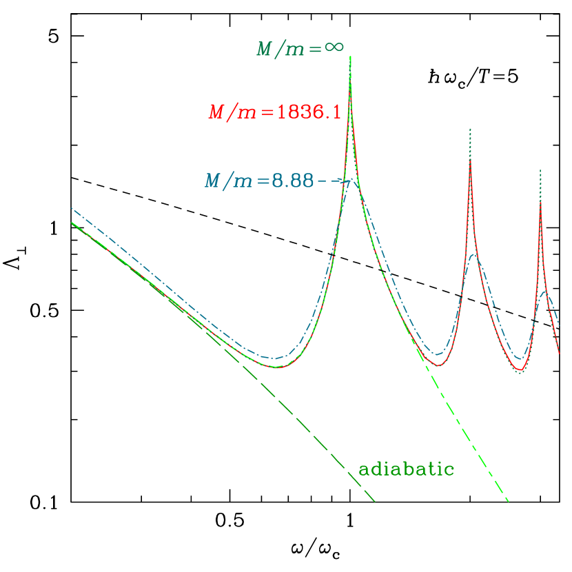
Figure 1: Transverse Coulomb logarithm as a function of $\omega/\omega_{\mathrm{c}}$ at $\hbar\omega_{\mathrm{c}}/T=5$ for different approximations: the model of fixed Coulomb potential (dotted line), approximate account of proton recoil (solid line), adiabatic approximation (long-dashed line), and the first post-adiabatic approximation (short dash - long dash). The divergent peaks are trimmed at $|\omega-(l+1)\,\omega_{\mathrm{c}}|=10^{-3}\omega_{\mathrm{c}}$ ($l=0,1,2,\ldots$). For comparison, the nonmagnetic Coulomb logarithm (short dashes; in this case the horizontal axis displays $\hbar\omega/5T$) and the model with approximate account of proton recoil in the muonic atom $\mu^{-}p$ (dot-dashed line) are shown.

Figure 2: The same as in Fig. 1 but for the longitudinal Coulomb logarithm. In this case, lines with the approximate account of proton recoil almost coincide with the line corresponding to the fixed-potential approximation.

This approximation was used in all models of the spectra of strongly magnetized neutron stars until the beginning of the 21st century (e.g., Pavlov et al. 1995; Zane et al. 2000, and references therein). It is validated by the large value of the mass ratio $M/m$. In addition, it requires that $\omega\gg\Omega_{\mathrm{c}}$, as seen directly from the comparison of Eq. (74) with Eq. (71).

5.1.2 Approximate account of proton recoil

Pavlov & Panov (1976) proposed an approximate treatment of proton recoil, which assumes that $\beta_{\mathrm{e}}\ll M/m$ and does not take into account Landau quantization of proton motion. In Fig. 1, the dotted line shows the perpendicular Coulomb logarithm $\Lambda_{\perp}^{\mathrm{ff}}$ calculated according to Eqs. (74)–(77), while the solid line takes the approximate account of proton recoil. As an example, we show the case where $\beta_{\mathrm{e}}=5$. The familiar nonmagnetic Coulomb logarithm in the first Born approximation (e.g., Bethe & Salpeter 1957) is shown by the short-dashed line, assuming the same $\hbar\omega/T$ along the horizontal axis as for the other curves ($\hbar\omega/T=\beta_{\mathrm{e}}\omega/\omega_{\mathrm{c}}$).

To enhance the difference caused by the recoil, we replace the electron by the muon $\mu^{-}$. All the above formulae and discussion remain unchanged, but now the mass ratio is $M/m=8.88$. The result of the approximate treatment of the recoil is shown by the dot-dashed line.

In Fig. 2, the same approximations are shown for $\Lambda_{\|}^{\mathrm{ff}}$. In this case, the lines related to the cyclotron harmonics are smoothed, because the factors $(u^{\prime}\pm u)^{2}$ quench the near-threshold growth of the integrand in Eq. (76). The same smoothing results in the infinite proton mass approximation being even more applicable (under the necessary condition $\omega\gg\Omega_{\mathrm{c}}$): the dotted, solid, and dot-dashed lines almost coincide in Fig. 2.

5.1.3 Adiabatic and post-adiabatic approximations

Several authors (Virtamo & Jauho 1975; Nagel & Ventura 1983; Mészáros 1992) used the adiabatic approximation not only for the unperturbed wave function $\psi^{(0)}$, but also for $\psi^{(1)}$. This was done in addition to assuming the infinite proton mass (Sect. 5.1.1). In other words, they kept only one $(n,s)$ term in the sum given by Eq. (40). The result is shown in Figs. 1 and 2 by long-dashed lines. We see that this approximation works well at $\omega\ll\omega_{\mathrm{c}}$, but becomes inaccurate at $\omega\gtrsim\omega_{\mathrm{c}}$.

Sawyer (2007) analyzed the photoabsorption problem by using the method of field theory. In the region $\Omega_{\mathrm{c}}\ll\omega\leq 1.5\omega_{\mathrm{c}}$, he considered account two electron Landau levels $n=0$ and 1 and applied a perturbation theory assuming the parameter $\varepsilon=\mathrm{e}^{-\beta_{\mathrm{e}}/2}$ to be small. His result is identical to the results discussed in Sect. 5.1.1 expanded in powers of $\varepsilon$, which we can write as

$$\Lambda_{\perp}^{\mathrm{ff}} = \frac{3}{4}\,\mathrm{e}^{\hbar\omega/T}\int_{0}^{\infty}\frac{\mathrm{d}y}{(1+y)^{2}}\,\Big{(}\,K_{0}(x_{0})$$ (78)

$$+\,\frac{2\mathrm{e}^{-\beta_{\mathrm{e}}/2}}{1+y}\big{(}K_{0}(x_{1})+K_{0}(x_{-1})\,\big{)}\,\Big{)}.$$

Here and in the next equation, $K_{\nu}(x_{n})$ are modified Bessel functions, and $x_{n}\equiv|\hbar\omega/T+n\beta_{\mathrm{e}}|\sqrt{0.25+y/\beta_{\mathrm{e}}}.$ Equation (78) differs from Eq. (28) of Sawyer (2007) in two respects: first, we have restored the factor 2 at $\mathrm{e}^{-\beta_{\mathrm{e}}/2}$, and second, we have dropped a term proportional to $\mathrm{e}^{-\beta_{\mathrm{e}}}$, because it is of the same order $\varepsilon^{2}$ as the contribution from the level $n=2$, and therefore should be treated together with the latter contribution in the next order of the perturbation theory.

In the same way, we obtain

$$\Lambda_{\|}^{\mathrm{ff}} = \frac{3}{4}\,\mathrm{e}^{\hbar\omega/T}\int_{0}^{\infty}\frac{\mathrm{d}y}{(1+y)\,(\beta_{\mathrm{e}}/4+y)}\,\Big{(}\,x_{0}\,K_{1}(x_{0})$$ (79)

$$+\,\frac{\mathrm{e}^{-\beta_{\mathrm{e}}/2}}{1+y}\big{(}x_{1}K_{1}(x_{1})+x_{-1}K_{1}(x_{-1})\,\big{)}\,\Big{)}.$$

Equations (78) and (79) can be obtained by the first iteration in the perturbation expansion, starting from the adiabatic aproximation.

5.2 Proton cyclotron harmonics

Proton cyclotron harmonics in the photoabsorption coefficients at $\omega=(l+1)\,\Omega_{\mathrm{c}}$ are superimposed on the peaks related to the electron cyclotron harmonics. However, for the H atom the two series of harmonics are separated because of the large value of $M/m=1836.1$. To observe the superimposition and the qualitative differences of various approximations, it is instructive to consider, in place of the H atom, the muonic atom (the $\mu^{-}p$ system), which has a smaller mass ratio $M/m=8.88$. The transverse Coulomb logarithm $\Lambda_{\perp}^{\mathrm{ff}}$ of photoabsorption by such system is shown in Fig. 3. The solid line displays the result of a calculation made according to Sect. 4. The other lines, as well as in Fig. 1, show the results of different approximations: a fixed Coulomb center (Sect. 5.1.1, dotted line), the approximate account of proton recoil (Sect. 5.1.2, dot-dashed line), and a nonmagnetic Coulomb logarithm (dashes).

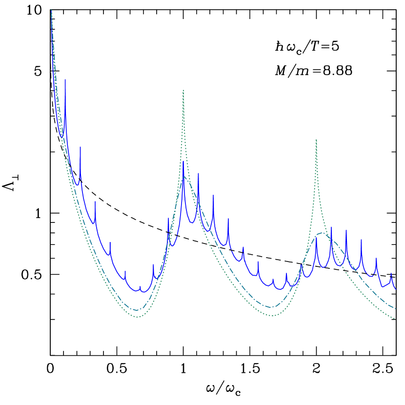
Figure 3: Transverse Coulomb logarithm as function of $\omega/\omega_{\mathrm{c}}$ at $\hbar\omega_{\mathrm{c}}/T=5$ in the model of fixed Coulomb potential (dotted line) and the approximate account of proton recoil (dot-dashed line), compared to the nonmagnetic Coulomb logarithm (dashed line) and the accurate calculation for the muonic atom $\mu^{-}p$ (solid line).

The smaller peaks in the solid curve correspond to the proton cyclotron harmonics. They are superimposed on the large-scale oscillations, which correspond to the muon cyclotron harmonics. Although the approximate recoil treatment (dot-dashed line) improves the agreement with the exact calculation compared to the infinite proton mass model (dotted line), both that approximate models that neglect proton Landau quantization differ significantly from the precise result.

In Fig. 4, we compare the proton cyclotron harmonics for different relative masses of the positive and negative particles. Here the proton cyclotron parameter is fixed to $\beta_{\mathrm{p}}=\hbar\Omega_{\mathrm{c}}/T=5$, and the horizontal axis displays the ratio $\omega/\Omega_{\mathrm{c}}$. The solid lines show the transverse Coulomb logarithm for the muonic atom (the lower curve) and the H atom (the upper curve). The dashed lines show $\Lambda_{\perp}^{\mathrm{ff}}$ calculated for the same $\hbar\omega_{\mathrm{c}}/T=\beta_{\mathrm{p}}M/m$ and the same $\omega/\omega_{\mathrm{c}}=(m/M)\,\omega/\Omega_{\mathrm{c}}$ as the solid curves, but for the approximation of a fixed Coulomb potential in the electron or muon scattering. By comparison, the dotted line shows $\Lambda_{\perp}^{\mathrm{ff}}$ calculated for proton scattering off a fixed Coulomb center, which can be regarded as a model where $M/m\to 0$. We see that the approximate models are unable to reproduce the proton cyclotron features correctly. It is also noteworthy that the larger the ratio $M/m$, the smaller the proton cyclotron peaks. In addition, the cyclotron resonance strength decreases with increasing harmonics number $l$. These properties of the cyclotron harmonics allow us to conclude that the solid lines in Figs. 1 and 2 are precise (proton cyclotron harmonics are negligible on their scale).

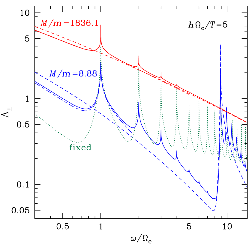
Figure 4: Transverse Coulomb logarithm as function of $\omega/\Omega_{\mathrm{c}}$ at $\hbar\Omega_{\mathrm{c}}/T=5$. The accurate calculation (solid line) for the systems $\mu^{-}p$ (lower lines) and $ep$ (upper lines) is compared to the approximation of a fixed Coulomb potential for the electron or muon scattering (dashed lines) or for the proton scattering (dotted line), and to the first post-adiabatic approximation (short dash - long dash).

In the early models of magnetized neutron star atmospheres (e.g., Pavlov & Shibanov 1978; Shibanov et al. 1992; Shibanov & Zavlin 1995), the authors considered moderate magnetic fields $B\sim 10^{11}$–$10^{12}$ G, where the proton Landau quantization is unimportant. More recently, observational evidence has accumulated that some of the isolated neutron stars are probably magnetars, which have fields of $B\sim 10^{14}$ G (see, e.g., the review by Mereghetti 2008 and references therein). According to Eq. (2), the proton cyclotron lines of magnetars are in an observationally accessible spectral range, which has encouraged theoretical modeling of these features. In the absence of an accurate quantum treatment, several authors (Zane et al. 2000, 2001; Özel 2001; Ho & Lai 2001, 2003) employed the scaling previously suggested for this purpose by Pavlov et al. (1995), according to which the free-free cross-section for protons equals $(m/M)^{2}\,\sigma_{-\alpha}(\omega M/m)$, where $\sigma_{\alpha}(\omega)$ is given by Eq. (74). The latter equation differs remarkably from the correct expression in Eq. (71). At photon frequencies $\omega<\Omega_{\mathrm{c}}$, the difference roughly amounts to a factor of $(\omega/\Omega_{\mathrm{c}})^{2}$.

In addition, the Coulomb logarithm that determines $\nu_{\alpha}^{\mathrm{ff}}$ cannot be obtained from this scaling. An example is shown in Fig. 4, where the dotted line corresponding to the fixed-potential model is compared with the accurate calculations displayed by the solid lines. We see that the fixed-potential model strongly overestimates the strength of the proton cyclotron harmonics. The origin of the discrepancy is clear: while considering a collision of a proton with an electron, one cannot assume the electron to be a nonmoving particle.

Sawyer (2007) employed a representation with definite $s_{\mathrm{e}}$ and $s_{\mathrm{p}}$ and analyzed the first proton-cyclotron peak of $\Lambda_{\perp}^{\mathrm{ff}}$, in a way similar to his analysis of the first electron cyclotron peak (see Sect. 5.1.3), by taking into account the ground electron Landau level $n=0$ and two proton Landau levels, $N=0$ and 1. The result (his Eq. 30) is quite accurate close to the fundamental cyclotron frequency, as we illustrate wuth the lines of alternating short and long dashes in Fig. 4. In the case of hydrogen (higher $M/m$), it almost coincides with the accurate result (solid line) at $\omega\lesssim 1.5\,\Omega_{\mathrm{c}}$ and with the result obtained by neglecting the Landau quantization of protons (dashed line) at higher $\omega$ values.

6 Discussion

6.1 Corrections beyond Born approximation

The formulae presented in Sects. 3.1 and 4.1 in principle allow one to perform an accurate calculation of photoabsorption rates in the electron-proton system in an arbitrary magnetic field, taking into account the effects of Landau quantization of the electron and proton motion across the field and the transverse motion of the center of mass. For bound-free absorption, this calculation was presented by Potekhin & Pavlov (1997). For free-free processes, we apply the first Born approximation and the dipole approximation. We plan to perform calculations of the free-free opacities beyond Born approximation in future work. An approximate estimate of the non-Born corrections can be obtained (Potekhin & Lai 2007) by introducing correction factors $(1+\gamma_{\ast}^{-1}u^{-2})^{-1/2}(1+\gamma_{\ast}^{-1}(u^{\prime})^{-2})^{-1/2}$ into the integral of Eq. (68), where $\gamma_{\ast}=(m/m_{\ast})^{2}\gamma$ and $\gamma=\hbar^{3}B/(m^{2}ce^{3})=425.44\,B_{12}.$ The accuracy of the approximation is ensured by the smallness of $\gamma_{\ast}^{-1/2}\approx 0.05\,B_{12}^{-1/2}$ and the additional condition $T\gg e^{4}m_{\ast}/\hbar^{2}$, which is the usual applicability condition for a Born approximation without a magnetic field.

We have checked that these corrections are sufficiently small for the electron cyclotron harmonics at $B\sim 10^{11}$ G (relevant to CCOs) and negligible for the proton cyclotron harmonics at $B>10^{13}$ G (relevant to XDINSs).

6.2 Importance of bound states

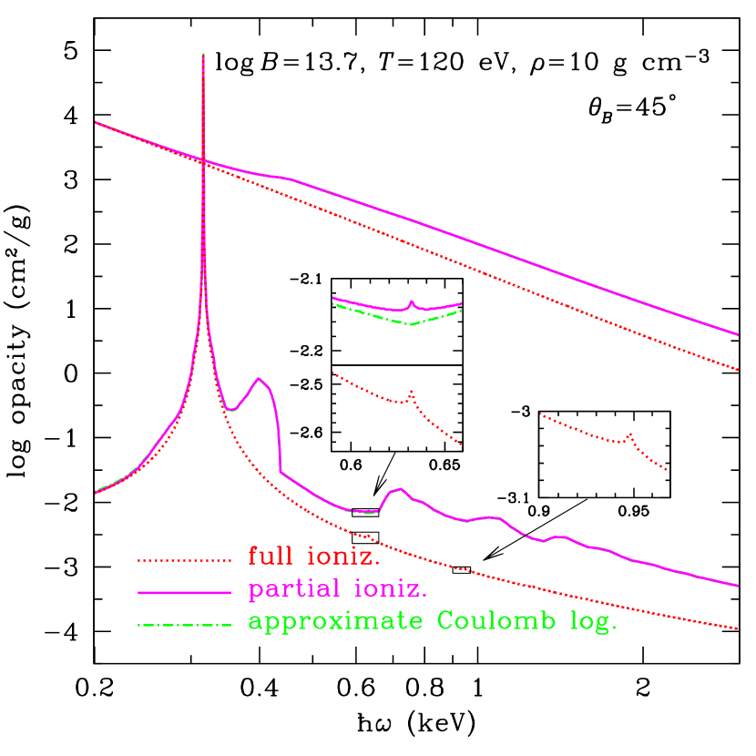
Figure 5: Opacities for the two normal electromagnetic waves propagating at the angle $\theta_{B}=45^{\circ}$ to the magnetic field direction in a hydrogen atmosphere of a neutron star with $B=5\times 10^{13}$ G and $T=120$ eV at density $\rho=10$ g cm^-3 (which is in the middle of the photosphere at these $B$ and $T$). The results are shown for fully ionized (dotted lines) and partially ionized (solid and dot-dashed lines) plasma models. In the latter model, the nonionized atomic fraction equals 0.0066. The solid line shows the opacity obtained with the accurate calculation of the free-free Coulomb logarithm, and the dot-dashed line demonstrates the result of the approximate treatment that corresponds to the dashed line in Fig. 4.

Free-free absorption contributes only a part of the total opacities in the atmospheres of neutron stars. A second constituent is the familiar scattering, and a third the absorption by bound species (see, e.g., Canuto & Ventura 1977; Pavlov et al. 1995). It was realized long ago (Ruderman 1971) that in strong magnetic fields the increase in the binding energies of atoms and molecules can lead to their non-negligible abundance even in hot atmospheres. With increasing $B$, the binding energies and abundances of bound species increase at any fixed density $\rho$ and temperature $T$ (Potekhin et al. 1999; Lai 2001), so that even the lightest of the atoms, hydrogen, provides a noticeable contribution to the opacities at the temperatures of interest, if the magnetic field is strong enough. Even a small neutral fraction can be important, because the bound-bound and bound-free cross-sections are large close to certain characteristic spectral energies.

For electron cyclotron harmonics to appear at $\hbar\omega\lesssim 1$ keV, we should ensure that $B\lesssim 10^{11}$ G according to Eq. (1). At these relatively weak magnetic fields and the characteristic temperature $T^{\infty}\gtrsim 100$ eV, the assumption of full ionization may be acceptable. However, at $B>10^{13}$ G, which is required for ion cyclotron harmonics, the situation is different. An illustration is given in Fig. 5. The solid curves show true absorption opacities for two normal electromagnetic waves propagating at the angle $45^{\circ}$ to the magnetic field lines at $B=5\times 10^{13}$ G and $T=120$ eV. The upper and lower curves correspond to the ordinary and extraordinary waves, respectively. The density in this example is chosen to be $\rho=10$ g cm^-3, which is a typical atmosphere density at $B=5\times 10^{13}$ G and $T_{\mathrm{eff}}^{\infty}=100$ eV (at this density the thermodynamic temperature $T$ approximately equals the effective temperature $T_{\mathrm{eff}}$). According to our ionization equilibrium model (Potekhin et al. 1999), at these $B$, $T$, and $\rho$ values, 0.66% of protons in the plasma are comprised in the ground-state H atoms that are not too strongly perturbed by plasma microfields so that they contribute to the bound-bound and bound-free opacities (the “optical” atomic fraction), and only 0.1% of protons are in excited bound states. Even though the ground-state atomic fraction is small, it is not negligible. In Fig. 5, at $\hbar\omega\gtrsim 0.4$ keV, the opacities in two normal modes, calculated with allowance for partial ionization (solid and dot-dashed curves), are significantly higher and have more characteristic features than the opacity calculated under the assumption of complete ionization (dotted lines). In particular, the broad feature on the lower curve near 0.4 keV is produced by the principal bound-bound transition between the two lowest bound states ($s_{i}=0\to s_{f}=1$), and the increased value of the opacity at higher energies $\hbar\omega$ is due to the transitions to other bound and free quantum states. The wavy shape of the lower solid curve (for the extraordinary mode) at $\hbar\omega\gtrsim 0.7$ keV is explained by bound-free transitions to different open channels, each having its own threshold energy. All the bound-bound absorption features and photoionization thresholds are strongly broadened by the effects of atomic motion across the magnetic field lines (“magnetic broadening”, see Potekhin & Pavlov 1997 and references therein).

In the insets, we zoom in on the regions of the first and second proton cyclotron harmonics. Both of them are visible, but negligible compared to the effect of partial ionization on the opacities.

6.3 Other possibilities for CCOs and XDINSs

Apart from the cyclotron harmonics, a number of alternative explanations of the observed absorption features in CCOs and XDINSs have been suggested in the literature.

Mori & Ho (2007) constructed models of strongly magnetized neutron star atmospheres with mid-$Z$ elements and compared them to the observed spectra of the neutron stars 1E 1207.4-5209 and RX J1605.3+3249. They demonstrated that the positions and relative strengths of the strongest absorption features in these neutron stars are in good agreement with a model of a strongly ionized oxygen atmosphere with $B=10^{12}$ G and $B=10^{13}$ G, respectively. This explanation seems promising, but unsolved problems remain: the effects of motion across the field have been treated approximately, based on the assumption that they are small, and detailed fits to the observed spectra have not yet been presented.

Among other hypotheses about the nature of the absorption features, there was a suggestion that they could be due to bound-bound transitions in exotic molecular ions (Turbiner & López Vieyra 2006). However, our estimates show that the abundance of these ions in a neutron star atmosphere would be negligible compared with the abundance of H atoms. Suleimanov et al. (2009) proposed a “sandwich” model atmosphere of finite depth, composed of a helium slab above a condensed surface and beneath hydrogen, and demonstrated that this model can produce two or three absorption features in the range of $\hbar\omega\sim 0.2$–1 keV at $B\sim 10^{14}$ G, although a detailed comparison with observed spectra was not performed. One cannot also rule out that some absorption lines originate in a cloud near a neutron star, rather than in the atmosphere (see Hambaryan et al. 2009).

7 Summary

We have considered the basic methods for calculation of free-free opacities of a magnetized hydrogen plasma. Our emphasis has been on the case where not only electron, but also proton motion across the magnetic field is quantized by the Landau states. We have derived general formulae for the photoabsorption rates and considered in detail the dipole, first Born approximation. We have presented numerical examples, compared them with the results of previously used simplified models, and analyzed the physical assumptions behind the different simplifications and conditions of their applicability. We have demonstrated that the proton cyclotron harmonics at a given value of the parameter $\beta_{\mathrm{p}}=\hbar\Omega_{\mathrm{c}}/T$ are much weaker than the respective electron cyclotron harmonics at the same value of $\beta_{\mathrm{e}}=\hbar\omega_{\mathrm{c}}/T$, and explained this difference in terms the large (nonperturbative) effects of proton motion in the case of proton cyclotron harmonics, in contrast to the case of the electron cyclotron harmonics.

References

• Araya & Harding (1999) Araya, R. A., & Harding, A. K. 1999, ApJ, 517, 334
• Araya-Góchez & Harding (2000) Araya-Góchez, R. A., & Harding, A. K. 2000, ApJ, 544, 1067
• Armstrong & Nicholls (1972) Armstrong, B. M., & Nicholls, R. W. 1972, Emission, Absorption and Transfer of Radiation in Heated Atmospheres (Pergamon, Oxford)
• Bekefi (1966) Bekefi, G. 1966, Radiation Processes in Plasmas (Wiley, New York)
• Bethe & Salpeter (1957) Bethe, H. A., & Salpeter, E. E. 1957, Quantum Mechanics of One- and Two-Electron Atoms (Springer, Berlin)
• Bezchastnov & Potekhin (1994) Bezchastnov, V. G., & Potekhin, A. Y. 1994, J. Phys. B, 27, 3349
• Bignami et al. (2003) Bignami, G. F., Caraveo, P. A., De Luca, A., & Mereghetti, S. 2003, Nature, 423, 725
• Canuto & Ventura (1977) Canuto, V., & Ventura, J. 1977, Fundam. Cosmic Phys., 2, 203
• Cohen-Tannoudji et al. (1998) Cohen-Tannoudji, C., Dupont-Roc, J., & Grynberg, G. 1998, Atom-Photon Interactions: Basic Processes and Applications (Wiley, Berlin)
• Cropper et al. (2007) Cropper, M., Zane, S., Turolla, R., et al. 2007, Ap&SS, 308, 161
• Daugherty & Ventura (1977) Daugherty, J. K., & Ventura, J. 1977, A&A, 61, 723
• de Luca (2008) de Luca, A. 2008, AIP Conf. Proc., 983, 311
• de Luca et al. (2004) de Luca, A., Mereghetti, S., Caraveo, P. A., et al. 2004, A&A, 418, 625
• Enoto et al. (2008) Enoto, T., Makishima, K., Terada, Y., et al. 2008, PASJ, 60, S57
• Ginzburg (1970) Ginzburg, V. L. 1970, The Propagation of Electromagnetic Waves in Plasmas, 2nd ed. (Pergamon, London)
• Gnedin & Syunyaev (1974) Gnedin, Yu. N., & Sunyaev, R. A. 1974, A&A, 36, 379
• Gor’kov & Dzyaloshinskii (1968) Gor’kov, L. P., & Dzyaloshinskii, I. E. 1968, Sov. Phys. JETP, 26, 449
• Haberl (2007) Haberl, F. 2007, Ap&SS, 308, 181
• Haberl et al. (2004) Haberl, F., Zavlin, V. E., Trümper, J., & Burwitz, V. 2004, A&A, 419, 1077
• Halpern & Gotthelf (2010) Halpern, J. P., & Gotthelf, E. V. 2010, ApJ, 709, 436
• Hambaryan et al. (2009) Hambaryan, V., Neuhäuser, R., Haberl, F., Hohle, M. M., & Schwope, A. D. 2009, A&A, 497, L9
• Ho & Lai (2001) Ho, W. C. G. & Lai, D. 2001, MNRAS, 327, 1081
• Ho & Lai (2003) Ho, W. C. G. & Lai, D. 2003, MNRAS, 338, 233
• Ho et al. (2008) Ho, W. C. G., Potekhin A. Y., & Chabrier, G. 2008, ApJS, 178, 102
• Hohle et al. (2009) Hohle, M. M., Haberl, F., Vink, J., et al. 2009, A&A, 498, 811
• Johnson & Lippmann (1949) Johnson, M. H., & Lippmann, B. A. 1949, Phys. Rev., 76, 828
• Johnson et al. (1983) Johnson, B. R., Hirschfelder, J. O., & Yang, K.-H. 1983, Rev. Mod. Phys., 55, 109
• Kaplan & van Kerkwijk (2009) Kaplan, D. L., & van Kerkwijk, M. H. 2009, ApJ, 692, L62
• Kaspi et al. (2006) Kaspi, V. M., Roberts, M. S. E., & Harding, A. K. 2006, in Compact Stellar X-Ray Sources, ed. W. Lewin & M. van der Klis (Cambridge University Press, Cambridge, UK), 279
• Kopidakis et al. (1996) Kopidakis, N., Ventura, J., & Herold, H. 1996, A&A, 308, 747
• Lai (2001) Lai, D., 2001, Rev. Mod. Phys., 73, 629
• Landau & Lifshitz (1976) Landau, L. D., & Lifshitz, E. M. 1976, Quantum Mechanics (Pergamon, Oxford)
• Mereghetti (2008) Mereghetti, S. 2008, A&A Rev., 15, 225
• Mészáros (1992) Mészáros, P., 1992, High-Energy Radiation from Magnetized Neutron Stars (Chicago: Univ. of Chicago Press)
• Mori & Ho (2007) Mori, K. & Ho, W. C. G. 2007, MNRAS, 377, 905
• Mori et al. (2005) Mori, K., Chonko, J. C., & Hailey, C. J. 2005, ApJ, 631, 1082
• Nagel & Ventura (1983) Nagel, W., & Ventura, J. 1983, A&A, 118, 66
• Nishimura (2005) Nishimura, O. 2005, PASJ, 57, 769
• Nishimura (2008) Nishimura, O. 2008, ApJ, 672, 1127
• Özel (2001) Özel, F. 2001, ApJ, 563, 276
• Pavlov & Panov (1976) Pavlov, G. G., & Panov, A. N. 1976, Sov. Phys. JETP, 44, 300
• Pavlov & Shibanov (1978) Pavlov, G. G., & Shibanov, Yu. A. 1978, Sov. Ast., 22, 214
• Pavlov et al. (1980) Pavlov, G. G., Shibanov, Yu. A., & Yakovlev, D.G. 1980, Ap&SS, 73, 33
• Pavlov et al. (1995) Pavlov, G. G., Shibanov, Yu. A., Zavlin, V. E., & Meyer, R. D. 1995, in The Lives of the Neutron Stars, NATO ASI Ser. C, 450, ed. M. A. Alpar, Ü. Kiziloğlu, & J. van Paradijs (Kluwer, Dordrecht), 71
• Potekhin (1994) Potekhin, A. Y. 1994, J. Phys. B, 27, 1073
• Potekhin (1998) Potekhin, A. Y. 1998, J. Phys. B, 31, 49