New Regularization in Extra Dimensional Model and Renormalization Group Flow of the Cosmological Constant

Abstract

Casimir energy is calculated for 5D scalar theory in the warped geometry. A new regularization, called sphere lattice regularization, is taken. The regularized configuration is closed-string like. We numerically evaluate $\Lambda$(4D UV-cutoff), $\omega$(5D bulk curvature, warp parameter) and $T$(extra space IR parameter) dependence of Casimir energy. 5D Casimir energy is finitely obtained after the proper renormalization procedure. The warp parameter $\omega$ suffers from the renormalization effect. We examine the cosmological constant problem.

Laboratory of Physics, School of Food and Nutritional Sciences, University of Shizuoka
Yada 52-1, Shizuoka 422-8526, Japan
ichinose@u-shizuoka-ken.ac.jp

1. Introduction In the quest for the unified theory, the higher dimensional (HD) approach is a fascinating one from the geometrical point. Historically the initial successful one is the Kaluza-Klein model, which unifies the photon, graviton and dilaton from the 5D space-time approach. The HD theories , however, generally have the serious defect as the quantum field theory(QFT) : un-renormalizability. The HD quantum field theories, at present, are not defined within the QFT.

In 1983, the Casimir energy in the Kaluza-Klein theory was calculated by Appelquist and Chodos[1]. They took the cut-off ($\Lambda$) regularization and found the quintic ($\Lambda^{5}$) divergence and the finite term. The divergent term shows the unrenormalizability of the 5D theory, but the finite term looks meaningful[2] and, in fact, is widely regarded as the right vacuum energy which shows contraction of the extra axis.

In the development of the string and D-brane theories, a new approach to the renormalization group was found. It is called holographic renormalization. We regard the renormalization flow as a curve in the bulk. The flow goes along the extra axis. The curve is derived as a dynamical equation such as Hamilton-Jacobi equation. It originated from the AdS/CFT correspondence. Spiritually the present basic idea overlaps with this approach.

2. Casimir Energy of 5D Scalar Theory In the warped geometry, $ds^{2}=\frac{1}{\omega^{2}z^{2}}(\eta_{\mu\nu}dx^{\mu}dx^{\nu}+{dz}^{2})$ , we consider the 5D massive scalar theory with $m^{2}=-4\omega^{2}$. ${\cal L}=\sqrt{-G}(-{\frac{1}{2}}\nabla^{A}\Phi\nabla_{A}\Phi-{\frac{1}{2}}m^{2}\Phi^{2})$ . The Casimir energy $E_{Cas}$ is given by

$$\mbox{e}^{-T^{-4}E_{Cas}}=\left.\int{\cal D}\Phi\exp\{i\int d^{5}X{\cal L}\}\right|_{\mbox{Euclid}}=\exp\sum_{n,p}\{-{\frac{1}{2}}\ln(p_{E}^{2}+M_{n}^{2})\}{\quad,}$$ (1)

where $M_{n}$ is the eigenvalues of the following operator.

$$\{s(z)^{-1}{\hat{L}}_{z}+{M_{n}}^{2}\}\psi_{n}(z)=0{\quad,}\quad{\hat{L}}_{z}\equiv\frac{d}{dz}\frac{1}{(\omega z)^{3}}\frac{d}{dz}-\frac{m^{2}}{(\omega z)^{5}}{\quad,}$$ (2)

where $s(z)=\frac{1}{(\omega z)^{3}}$. Z₂ parity is imposed as: $\psi_{n}(z)=-\psi_{n}(-z)\ \mbox{for}\ P=-\ ;\ \psi_{n}(z)=\psi_{n}(-z)\ \mbox{for}\ P=+$. The expression (1) is the familiar one of the Casimir energy. It is re-expressed in a closed form using the heat-kernel method and the propagator. First we can express it, using the heat equation solution, as follows ($\omega/T=\mbox{e}^{\omega l}$).

$$\mbox{e}^{-T^{-4}E_{Cas}}=(\mbox{const})\times\exp\left[T^{-4}{\int\frac{d^{4}p}{(2\pi)^{4}}}2\int_{0}^{\infty}{\frac{1}{2}}\frac{dt}{t}\mbox{Tr}~{}H_{p}(z,z^{\prime};t)\right]{\quad,}$$

$$\mbox{Tr}~{}H_{p}(z,z^{\prime};t)=\int_{1/\omega}^{1/T}s(z)H_{p}(z,z;t)dz{\quad,}\quad\{\frac{\partial}{\partial t}-(s^{-1}{\hat{L}}_{z}-p^{2})\}H_{p}(z,z^{\prime};t)=0{\quad.}$$ (3)

The heat kernel $H_{p}(z,z^{\prime};t)$ is formally solved, using the Dirac’s bra and ket vectors $(z|,|z)$, as  $H_{p}(z,z^{\prime};t)=(z|\mbox{e}^{-(-s^{-1}{\hat{L}}_{z}+p^{2})t}|z^{\prime})$. We here introduce the position/momentum propagators $G^{\mp}_{p}$: $G^{\mp}_{p}(z,z^{\prime})\equiv\int_{0}^{\infty}dt~{}H_{p}(z,z^{\prime};t)$. They satisfy the following differential equations of propagators.

$$({\hat{L}}_{z}-p^{2}s(z))G^{\mp}_{p}(z,z^{\prime})=\left\{\begin{array}[]{ll}\epsilon(z)\epsilon(z^{\prime}){\hat{\delta}}(|z|-|z^{\prime}|)&\mbox{\ P=}-1\\ {\hat{\delta}}(|z|-|z^{\prime}|)&\mbox{\ P=}1\end{array}\right.$$ (6)

$G_{p}^{\mp}$ can be expressed in a closed form. Taking the Dirichlet condition at all fixed points, the expression for the fundamental region ($1/\omega\leq z\leq z^{\prime}\leq 1/T$) is given by

$$G_{p}^{\mp}(z,z^{\prime})=\mp\frac{\omega^{3}}{2}z^{2}{z^{\prime}}^{2}\frac{\{{\bf I}_{0}(\frac{{\tilde{p}}}{\omega}){\bf K}_{0}({\tilde{p}}z)\mp{\bf K}_{0}(\frac{{\tilde{p}}}{\omega}){\bf I}_{0}({\tilde{p}}z)\}\{{\bf I}_{0}(\frac{{\tilde{p}}}{T}){\bf K}_{0}({\tilde{p}}z^{\prime})\mp{\bf K}_{0}(\frac{{\tilde{p}}}{T}){\bf I}_{0}({\tilde{p}}z^{\prime})\}}{{\bf I}_{0}(\frac{{\tilde{p}}}{T}){\bf K}_{0}(\frac{{\tilde{p}}}{\omega})-{\bf K}_{0}(\frac{{\tilde{p}}}{T}){\bf I}_{0}(\frac{{\tilde{p}}}{\omega})},$$ (7)

where ${\tilde{p}}\equiv\sqrt{p^{2}},p^{2}\geq 0$. We can express Casimir energy as,

$$-E^{\Lambda,\mp}_{Cas}(\omega,T)=\left.{\int\frac{d^{4}p_{E}}{(2\pi)^{4}}}\right|_{{\tilde{p}}\leq\Lambda}\int_{1/\omega}^{1/T}dz~{}F^{\mp}({\tilde{p}},z),F^{\mp}({\tilde{p}},z)=\frac{2}{(\omega z)^{3}}\int_{\tilde{p}}^{\Lambda}{\tilde{k}}~{}G^{\mp}_{k}(z,z)d{\tilde{k}},$$ (8)

where ${\tilde{p}}=\sqrt{p_{E}^{2}}$. The momentum symbol $p_{E}$ indicates Euclideanization. Here we introduce the UV cut-off parameter $\Lambda$ for the 4D momentum space.

3. UV and IR Regularization and Evaluation of Casimir Energy The integral region of the above equation (8) is displayed in Fig.1. In the figure, we introduce the regularization cut-offs for the 4D-momentum integral, $\mu\leq{\tilde{p}}\leq\Lambda$. For simplicity, we take the following IR cutoff of 4D momentum : $\mu=\Lambda\cdot\frac{T}{\omega}=\Lambda\mbox{e}^{-\omega l}$ .

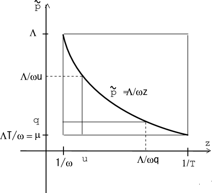
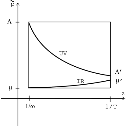
Figure 1: Space of (z,${\tilde{p}}$) for the integration. The hyperbolic curve was proposed[3].

Figure 2: Space of (${\tilde{p}}$,z) for the integration (present proposal).

Importantly, (8) shows the scaling behavior for large values of $\Lambda$ and $1/T$. From a close numerical analysis, we have confirmed : (4A) $E^{\Lambda,-}_{Cas}(\omega,T)=\frac{2\pi^{2}}{(2\pi)^{4}}\times\left[-0.0250\frac{\Lambda^{5}}{T}\right]$. The $\Lambda^{5}$-divergence, (4A), shows the notorious problem of the higher dimensional theories. We have proposed an approach to solve this problem and given a legitimate explanation within the 5D QFT[4, 5]. See Fig.2. The IR and UV cutoffs change along the etra axis. Their $S^{3}$-radii are given by $r_{IR}(z)$ and $r_{UV}(z)$. The 5D volume region bounded by $B_{UV}$ and $B_{IR}$ is the integral region of the Casimir energy $E_{Cas}$. The forms of $r_{UV}(z)$ and $r_{IR}(z)$ can be determined by the minimal area principle: $3+\frac{4}{z}r^{\prime}r-\frac{r^{\prime\prime}r}{{r^{\prime}}^{2}+1}=0,r^{\prime}\equiv\frac{dr}{dz},r^{\prime\prime}\equiv\frac{d^{2}r}{dz^{2}},1/\omega\leq z\leq 1/T$. We have confirmed, by numerically solving the above differential eqation (Runge-Kutta), those curves that show the flow of renormalization really appear. The results imply the boundary conditions determine the property of the renormalization flow.

4. Weight Function and the Meaning We consider another approach which respects the minimal area principle. Let us introduce, instead of restricting the integral region, a weight function $W({\tilde{p}},z)$ in the (${\tilde{p}},z$)-space for the purpose of suppressing UV and IR divergences of the Casimir Energy.

$$-E^{\mp~{}W}_{Cas}(\omega,T)\equiv{\int\frac{d^{4}p_{E}}{(2\pi)^{4}}}\int_{1/\omega}^{1/T}dz~{}W({\tilde{p}},z)F^{\mp}({\tilde{p}},z){\quad,}\quad{\tilde{p}}=\sqrt{p_{4}^{2}+p_{1}^{2}+p_{2}^{2}+p_{3}^{2}}{\quad,}$$

$$\left\{\begin{array}[]{cc}(N_{1})^{-1}\mbox{e}^{-(1/2){\tilde{p}}^{2}/\omega^{2}-(1/2)z^{2}T^{2}}\equiv W_{1}({\tilde{p}},z),\ N_{1}=1.711/8\pi^{2}&\mbox{elliptic suppr.}\\ (N_{2})^{-1}\mbox{e}^{-{\tilde{p}}zT/\omega}\equiv W_{2}({\tilde{p}},z),\ N_{2}=2\frac{\omega^{3}}{T^{3}}/8\pi^{2}&\mbox{hyperbolic suppr.1}\\ (N_{8})^{-1}\mbox{e}^{-1/2({\tilde{p}}^{2}/\omega^{2}+1/z^{2}T^{2})}\equiv W_{8}({\tilde{p}},z),\ N_{8}=0.4177/8\pi^{2}&\mbox{reciprocal suppr.1}\\ \end{array}\right.$$ (12)

where $F^{\mp}({\tilde{p}},z)$ are defined in (8). They (except $W_{2}$) give, after normalizing the factor $\Lambda/T$, only the log-divergence.

$$E^{W}_{Cas}/\Lambda T^{-1}=-\alpha\omega^{4}\left(1-4c\ln(\Lambda/\omega)-4c^{\prime}\ln(\Lambda/T)\right){\quad,}$$ (13)

where the numerical values of $\alpha,c$ and $c^{\prime}$ are obtained depending on the choice of the weight function[6]. This means the 5D Casimir energy is finitely obtained by the ordinary renormalization of the warp factor $\omega$.

In the previous work[5], we have presented the following idea to define the weight function $W({\tilde{p}},z)$. In the evaluation (12), the $({\tilde{p}},z)$-integral is over the rectangle region shown in Fig.1 (with $\Lambda\rightarrow\infty$ and $\mu\rightarrow 0$). Following Feynman[7], we can replace the integral by the summation over all possible pathes ${\tilde{p}}(z)$.

$$-E^{W}_{Cas}(\omega,T)=\int{\cal D}{\tilde{p}}(z)\int_{1/\omega}^{1/T}dz~{}S[{\tilde{p}}(z),z],S[{\tilde{p}}(z),z]=\frac{2\pi^{2}}{(2\pi)^{4}}{\tilde{p}}(z)^{3}W({\tilde{p}}(z),z)F^{\mp}({\tilde{p}}(z),z).$$ (14)

There exists the dominant path ${\tilde{p}}_{W}(z)$ which is determined by the minimal principle : $\delta S=0$. Dominant Path ${\tilde{p}}_{W}(z)\ :\ \quad$ $\frac{d{\tilde{p}}}{dz}=$ $-\frac{\partial\ln(WF)}{\partial z}$/ $(\frac{3}{{\tilde{p}}}+\frac{\partial\ln(WF)}{\partial{\tilde{p}}})$. Hence it is fixed by $W({\tilde{p}},z)$. On the other hand, there exists another independent path: the minimal surface curve $r_{g}(z)$. Minimal Surface Curve $r_{g}(z)$ : $3+\frac{4}{z}r^{\prime}r-\frac{r^{\prime\prime}r}{{r^{\prime}}^{2}+1}=0$, $\frac{1}{\omega}\leq z\leq\frac{1}{T}$. It is obtained by the minimal area principle: $\delta A=0$ where

$$ds^{2}=(\delta_{ab}+\frac{x^{a}x^{b}}{(rr^{\prime})^{2}})\frac{dx^{a}dx^{b}}{\omega^{2}z^{2}}\equiv g_{ab}(x)dx^{a}dx^{b},A=\int\sqrt{g}~{}d^{4}x=\int_{1/\omega}^{1/T}\frac{\sqrt{{r^{\prime}}^{2}+1}~{}r^{3}}{\omega^{4}z^{4}}dz.$$ (15)

Hence $r_{g}(z)$ is fixed by the induced geometry $g_{ab}(x)$. Here we put the requirement[5]: (4A) ${\tilde{p}}_{W}(z)={\tilde{p}}_{g}(z)$, where ${\tilde{p}}_{g}\equiv 1/r_{g}$. This means the following things. We require the dominant path coincides with the minimal surface line ${\tilde{p}}_{g}(z)=1/r_{g}(z)$ which is defined independently of $W({\tilde{p}},z)$. $W({\tilde{p}},z)$ is defined here by the induced geometry $g_{ab}(x)$. In this way, we can connect the integral-measure over the 5D-space with the geometry. We have confirmed the coincidence by the numerical method.

In order to most naturally accomplish the above requirement, we can go to a new step. Namely, we propose to replace the 5D space integral with the weight $W$, (12), by the following path-integral. We newly define the Casimir energy in the higher-dimensional theory as follows.

$$-{\cal E}_{Cas}(\omega,T,\Lambda)=\int_{1/\Lambda}^{1/\mu}d\rho\int{\begin{array}[]{l}r(\omega^{-1})\\ =r(T^{-1})\\ =\rho\end{array}}\prod_{a,z}{\cal D}x^{a}(z)F(\frac{1}{r},z)\exp\left[-\int_{1/\omega}^{1/T}\frac{\sqrt{{r^{\prime}}^{2}+1}~{}r^{3}}{2\alpha^{\prime}\omega^{4}z^{4}}dz\right],$$ (19)

where $\mu=\Lambda T/\omega$ and the limit $\Lambda T^{-1}\rightarrow\infty$ is taken. The string (surface) tension parameter $1/2\alpha^{\prime}$ is introduced. (Note: Dimension of $\alpha^{\prime}$ is [Length]⁴. ) $F({\tilde{p}},z)$ is defined in (8) and shows the field-quantization of the bulk scalar (EM) fields.

5. Discussion and Conclusion When $c$ and $c^{\prime}$ are sufficiently small we find the renormalization group function for the warp factor $\omega$ as

$$\omega_{r}=\omega(1-c\ln(\Lambda/\omega)-c^{\prime}\ln(\Lambda/T))\ ,\ \beta\equiv\frac{\partial}{\partial(\ln\Lambda)}\ln\frac{\omega_{r}}{\omega}=-c-c^{\prime}{\quad.}$$ (20)

No local counterterms are necessary.

Through the Casimir energy calculation, in the higher dimension, we find a way to quantize the higher dimensional theories within the QFT framework. The quantization with respect to the fields (except the gravitational fields $G_{AB}(X)$) is done in the standard way. After this step, the expression has the summation over the 5D space(-time) coordinates or momenta $\int dz\prod_{a}dp^{a}$. We have proposed that this summation should be replaced by the path-integral $\int\prod_{a,z}{\cal D}p^{a}(z)$ with the area action (Hamiltonian) $A=\int\sqrt{\det g_{ab}}d^{4}x$ where $g_{ab}$ is the induced metric on the 4D surface. This procedure says the 4D momenta $p^{a}$ (or coordinates $x^{a}$) are quantum statistical operators and the extra-coordinate $z$ is the inverse temperature (Euclidean time). We recall the similar situation occurs in the standard string approach. The space-time coordinates obey some uncertainty principle[8].

Recently the dark energy (as well as the dark matter) in the universe is a hot subject. It is well-known that the dominant candidate is the cosmological term. The cosmological constant $\lambda$ appears as: (5A) $R_{\mu\nu}-{\frac{1}{2}}g_{\mu\nu}R-\lambda g_{\mu\nu}=T_{\mu\nu}^{matter},S=\int d^{4}x\sqrt{-g}\{\frac{1}{G_{N}}(R+\lambda)\}+\int d^{4}x\sqrt{-g}\{{\cal L}_{matter}\},g=\mbox{det}~{}g_{{\mu\nu}}$ . We consider here the 3+1 dim Lorentzian space-time ($\mu,\nu=0,1,2,3$). The constant $\lambda$ observationally takes the value : (5B) $\frac{1}{G_{N}}\lambda_{obs}\sim\frac{1}{G_{N}{R_{cos}}^{2}}\sim m_{\nu}^{4}\sim(10^{-3}eV)^{4},\lambda_{obs}\sim\frac{1}{R_{cos}^{~{}2}}\sim 4\times 10^{-66}(eV)^{2}$, where $R_{cos}\sim 5\times 10^{32}\mbox{eV}^{-1}$ is the cosmological size (Hubble length), $m_{\nu}$ is the neutrino mass. On the other hand, we have theoretically so far : (5C) $\frac{1}{G_{N}}\lambda_{th}\sim\frac{1}{{G_{N}}^{2}}={M_{pl}}^{4}\sim(10^{28}eV)^{4}$. We have the famous huge discrepancy factor : (5D) $\frac{\lambda_{th}}{\lambda_{obs}}\sim N_{DL}^{~{}2},N_{DL}\equiv M_{pl}R_{cos}\sim 6\times 10^{60}$, where $N_{DL}$ is the Dirac’s large number. If we use the present result, we can obtain a natural choice of $T,\omega$ and $\Lambda$ as follows. By identifying $T^{-4}E_{Cas}=-\alpha_{1}\Lambda T^{-1}\omega^{4}/T^{4}$ with $\int d^{4}x\sqrt{-g}(1/G_{N})\lambda_{ob}=R_{cos}^{~{}2}(1/G_{N})$, we obtain the following relation: (5E) $N_{DL}^{~{}2}=R_{cos}^{~{}2}\frac{1}{G_{N}}=-\alpha_{1}\frac{\omega^{4}\Lambda}{T^{5}}$. The warped (AdS₅) model predicts the cosmological constant negative, hence we have interest only in its absolute value. We take the following choice for $\Lambda$ and $\omega$ : (5F) $\Lambda=M_{pl}\sim 10^{19}GeV,\omega\sim\frac{1}{\sqrt[4]{G_{N}{R_{cos}}^{2}}}=\sqrt{\frac{M_{pl}}{R_{cos}}}\sim m_{\nu}\sim 10^{-3}\mbox{eV}$.

As shown above, we have the standpoint that the cosmological constant is mainly made from the Casimir energy. We do not yet succeed in obtaining the value $\alpha_{1}$ negatively, but succeed in obtaining the finiteness of the cosmological constant and its gross absolute value. The smallness of the value is naturally explained by the renormalization flow. Because we already know the warp parameter $\omega$ flows (20), the $\lambda_{obs}\sim 1/R_{cos}^{2}\propto\omega^{4}$, says that the smallness of the cosmological constant comes from the renormalization flow for the non asymptotic-free case ($c+c^{\prime}<0$ in (20)).

The IR parameter $T$, the normalization factor $\Lambda/T$ in (13) and the IR cutoff $\mu=\Lambda\frac{T}{\omega}$ are given by : (5G) $T=R_{cos}^{~{}-1}(N_{DL})^{1/5}\sim 10^{-20}eV,\frac{\Lambda}{T}=(N_{DL})^{4/5}\sim 10^{50},\mu=M_{pl}N_{DL}^{-3/10}\sim 1GeV\sim m_{N}$, where $m_{N}$ is the nucleon mass. The degree of freedom of the universe (space-time) is given by : (5H) $\frac{\Lambda^{4}}{\mu^{4}}=\frac{\omega^{4}}{T^{4}}=N_{DL}^{~{}6/5}\sim 10^{74}\sim(\frac{M_{pl}}{m_{N}})^{4}$.

References

[1] T. Appelquist and A. Chodos, Phys.Rev.Lett.50(1983)141
[2] S. Ichinose, Phys.Lett.152B(1985),56
[3] L. Randall and M.D. Schwartz, JHEP0111 (2001) 003, hep-th/0108114
[4] S. Ichinose and A. Murayama, Phys.Rev.D76(2007)065008, hep-th/0703228
[5] S. Ichinose, Prog.Theor.Phys.121(2009)727, ArXiv:0801.3064v8[hep-th]