Chiral Gauge Theory for Graphene Edge

Abstract

An effective-mass theory with a deformation-induced (an axial) gauge field is proposed as a theoretical framework to study graphene edge. Though the gauge field is singular at edge, it can represent the boundary condition and this framework is adopted to solve the scattering problems for the zigzag and armchair edges. Furthermore, we solve the scattering problem in the presence of a mass term and an electromagnetic field. It is shown that the mass term makes the standing wave at the Dirac point avoid the zigzag edge, by which the local density of states disappears, and the lowest and first Landau states are special near the zigzag edge. The (chiral) gauge theory framework provides a useful description of graphene edge.

I Introduction

The graphene edge has attracted much attention, Kosynkin et al. (2009); Jiao et al. (2009); Jia et al. (2009); Girit et al. (2009); Liu et al. (2009); Stampfer et al. (2009); Han et al. (2010); Gallagher et al. (2010) because it is the source of a wide variety of notable phenomena. For example, the zigzag edge possesses localized edge states. Tanaka et al. (1987); Kobayashi (1993); Fujita et al. (1996); Nakada et al. (1996) The edge states enhance the local density of states near the Fermi energy. Klusek et al. (2000); Giunta and Kelty (2001); Kobayashi et al. (2005); Niimi et al. (2005) As a result, the spins of the edge states may be polarized by coulombic interaction. Fujita et al. (1996) Another type of edge, the armchair edge, does not support edge states. The zigzag edge is the source of intravalley scattering, while the armchair edge gives rise to intervalley scattering. The transport properties near the armchair edge may differ significantly from that near the zigzag edge; Wakabayashi et al. (2007); Yamamoto et al. (2009) however, the reason for this variety is unclear.

The Schrödinger equation is a differential equation; therefore, an appropriate boundary condition should be imposed on the equation. The boundary condition is sensitive to the situation of the edge, while the local dynamics, as described by the Schrödinger equation, are the same everywhere in a graphene sample. The wave function and energy spectrum are dependent on the boundary condition. In this sense, the boundary condition is the origin of the variety. Berry et al. (1987); McCann and Fal’ko (2004); Akhmerov and Beenakker (2007, 2008) In this paper, we attempt to construct a theoretical framework in which the edge is taken into account as a gauge field, and not as a boundary condition for the wave function. We show that the framework is useful to obtain and understand the standing wave and edge states.

This paper is organized as follows. In Sec. II, the qualitative features of the reflections from the zigzag and armchair edges are shown using the kinematics for elastic scattering. In Sec. III a general form of the electronic Hamiltonian is given for a graphene sheet with edges. In Secs. IV and V, the scattering problem is solved for both the zigzag and armchair edges, and the standing wave solution is obtained. A discussion and summary are given in Sec. VI.

II Reflection of Pseudospin

In the inset of Fig. 1, we consider the zigzag edge parallel to the $x$-axis, by which translational symmetry along the $y$-axis is broken. Thus, the incident state with wave vector $(k_{x},k_{y})$ is elastically scattered by the zigzag edge, and the wave vector of the reflected state becomes $(k_{x},-k_{y})$. In contrast, the armchair edge parallel to the $y$-axis breaks the translational symmetry along the $x$-axis, so that the wave vector of the reflected state is $(-k_{x},k_{y})$. The Brillouin zone (BZ) is given by 90^∘ rotation of the hexagonal lattice, so that for the incident state near the K point in Fig. 1, the zigzag edge reflected state is also near the K point, while the armchair edge reflected state is near the K^′ point. Therefore, scattering by the zigzag edge is intravalley scattering, while that by the armchair edge is intervalley scattering.

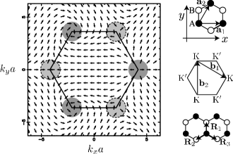
Figure 1: The pseudospin vector field in graphene BZ. Note that this field is for the conduction band and the pseudospin field for the valence band is given by reversing the direction of each arrow. The singularities in this pseudospin field correspond to the K or K^′ points. Appendix A outlines why the pseudospins at the (three) equivalent K (K^′) points are not identical. [inset-top] The hexagonal unit cell of graphene consists of A (solid circle) and B (open circle) atoms. The $xy$ coordinate system is fixed as shown. The vectors ${\bf a}_{1}$ and ${\bf a}_{2}$ are primitive translations. The length of each of these is $a$ ($a\equiv\sqrt{3}a_{\rm cc}$, where $a_{\rm cc}$ is the C-C bond length). [inset-middle] The vectors ${\bf b}_{1}$ and ${\bf b}_{2}$ are reciprocal lattice vectors defined by ${\bf a}_{i}\cdot{\bf b}_{j}=2\pi\delta_{ij}$. [inset-bottom] The vectors ${\bf R}_{a}$ are expressed as ${\bf R}_{1}=a_{\rm cc}{\bf e}_{y}$, ${\bf R}_{2}=-(\sqrt{3}/2)a_{\rm cc}{\bf e}_{x}-(1/2)a_{\rm cc}{\bf e}_{y}$, and ${\bf R}_{3}=(\sqrt{3}/2)a_{\rm cc}{\bf e}_{x}-(1/2)a_{\rm cc}{\bf e}_{y}$, where ${\bf e}_{x}$ (${\bf e}_{y}$) is the dimensionless unit vector for the $x$-axis ($y$-axis).

Pseudospin is defined as the expected value of the Pauli matrices $\sigma_{x,y,z}$ with respect to the two component Bloch function. The pseudospin provides information concerning the relative phase and the relative amplitude between the two components of the Bloch function, and it can be used to characterize scattering at the edges. Sasaki et al. (2010a) The Bloch function of the conduction state with wave vector ${\bf k}=(k_{x},k_{y})$ is given by

$$\Psi^{c}_{\bf k}=\frac{1}{\sqrt{2}}\begin{pmatrix}1\cr-\frac{f_{\bf k}^{*}}{|f_{\bf k}|}\end{pmatrix},$$ (1)

where $f_{\bf k}=\sum_{a}e^{i{\bf k}\cdot{\bf R}_{a}}$, $f_{\bf k}^{*}$ denotes the complex conjugate of $f_{\bf k}$, and ${\bf R}_{a}$ ($a=1,2,3$) are the vectors pointing to the nearest-neighbor B atoms from an A atom [see the inset of Fig. 1]. The pseudospin is then given by

$$\langle\sigma_{x}\rangle_{\bf k}=-\frac{{\rm Re}[f_{\bf k}]}{|f_{\bf k}|},\ \ \langle\sigma_{y}\rangle_{\bf k}=\frac{{\rm Im}[f_{\bf k}]}{|f_{\bf k}|},\ \ \langle\sigma_{z}\rangle_{\bf k}=0,$$ (2)

where

$$\begin{split}&{\rm Re}[f_{\bf k}]=\cos\left(\frac{k_{y}a}{\sqrt{3}}\right)+2\cos\left(\frac{k_{y}a}{2\sqrt{3}}\right)\cos\left(\frac{k_{x}a}{2}\right),\\ &{\rm Im}[f_{\bf k}]=\sin\left(\frac{k_{y}a}{\sqrt{3}}\right)-2\sin\left(\frac{k_{y}a}{2\sqrt{3}}\right)\cos\left(\frac{k_{x}a}{2}\right).\end{split}$$ (3)

The pseudospin, $(\langle\sigma_{x}\rangle_{\bf k},\langle\sigma_{y}\rangle_{\bf k},\langle\sigma_{z}\rangle_{\bf k})$, may be regarded as a two-dimensional vector field, because $\langle\sigma_{z}\rangle_{\bf k}=0$. The arrows in Fig. 1 show the pseudospin field, $(\langle\sigma_{x}\rangle_{\bf k},\langle\sigma_{y}\rangle_{\bf k})$. $\langle\sigma_{y}\rangle_{\bf k}$ is proportional to ${\rm Im}[f_{\bf k}]$; therefore, the angle of each arrow with respect to the $k_{x}$-axis represents the relative phase of the Bloch function between A and B atoms. For example, at the $\Gamma$ point ${\bf k}=0$ in Fig. 1, the arrow is pointing toward the negative $k_{x}$-axis. This implies that the wave function forms an antisymmetric combination with respect to the A and B atoms, which can be checked by setting ${\bf k}=0$ in Eq. (1). Since $\langle\sigma_{y}\rangle_{\bf k}$ is an odd function of $k_{y}$ as shown in Eq. (3), the pseudospin in Fig. 1 at $(k_{x},k_{y})$ and that at $(k_{x},-k_{y})$ point to different orientations with respect to $\langle\sigma_{y}\rangle$. In contrast, the pseudospin at $(k_{x},k_{y})$ and that at $(-k_{x},k_{y})$ point toward the same orientation. Thus, the pseudospin component perpendicular to the zigzag edge flips, while the pseudospin is invariant for the armchair edge.

We have seen for the zigzag edge that the reflection is intravalley scattering and that the pseudospin component perpendicular to the edge flips. For the armchair edge, the reflection is intervalley scattering and the pseudospin is invariant. More details concerning the scattering, for example, the relative phase between the incident and reflected waves and the edge states are difficult to obtain within the above argument. In subsequent sections we will explore an effective Hamiltonian to obtain the standing wave and the edge states.

III Deformation-induced gauge field

The fact that the pseudospin flips at the zigzag edge leads us to consider a gauge field for the edge that couples with the pseudospin in a manner similar to that an electromagnetic gauge field couples with the real spin. Here, we show the formulation, in which the effect of the edge is included into the Hamiltonian as a deformation-induced gauge field. Sasaki and Saito (2008a)

To begin with, we consider a change of the nearest-neighbor hopping integral from the average value, $-\gamma_{0}$, as $-\gamma_{0}+\delta\gamma_{0,a}({\bf r})$, where $a$ $(=1,2,3)$ denotes the direction of a bond parallel to ${\bf R}_{a}$ in the inset of Fig. 1. The deviation $\delta\gamma_{0,a}({\bf r})$ represents a lattice deformation in a graphene sheet. The low energy effective-mass equation for deformed graphene is written as

$$H({\bf r})\begin{pmatrix}\Psi_{\rm K}({\bf r})\cr\Psi_{\rm K^{\prime}}({\bf r})\end{pmatrix}=E\begin{pmatrix}\Psi_{\rm K}({\bf r})\cr\Psi_{\rm K^{\prime}}({\bf r})\end{pmatrix},$$ (4)

where $\Psi_{\rm K}({\bf r})$ and $\Psi_{\rm K^{\prime}}({\bf r})$ are two-component wavefunctions that represent the electrons near the K and K^′ points, respectively. The Hamiltonian for deformed graphene is written as Sasaki and Saito (2008a)

$$H({\bf r})=v_{\rm F}\begin{pmatrix}\mbox{\boldmath$\sigma$}\cdot({\bf{\hat{p}}}+{\bf A}^{\rm q}({\bf r}))&\phi^{\rm q}({\bf r})\sigma_{x}\cr\phi^{\rm q}({\bf r})^{*}\sigma_{x}&\mbox{\boldmath$\sigma$}^{\prime}\cdot({\bf{\hat{p}}}-{\bf A}^{\rm q}({\bf r}))\end{pmatrix},$$ (5)

where ${\hat{\bf p}}=-i\hbar\nabla$ is the momentum operator, $\mbox{\boldmath$\sigma$}=(\sigma_{x},\sigma_{y})$, and $\mbox{\boldmath$\sigma$}^{\prime}=(-\sigma_{x},\sigma_{y})$. A lattice deformation $\delta\gamma_{0,a}({\bf r})$ enters the Hamiltonian through the deformation-induced gauge field ${\bf A}^{\rm q}({\bf r})=(A_{x}^{\rm q}({\bf r}),A_{y}^{\rm q}({\bf r}))$, where ${\bf A}^{\rm q}({\bf r})$ is expressed by a linear combination of $\delta\gamma_{0,a}(\bf{r})$ as Kane and Mele (1997); Sasaki and Saito (2008a); Katsnelson and Geim (2008)

$$\begin{split}&v_{\rm F}A^{\rm q}_{x}({\bf r})=\delta\gamma_{0,1}({\bf r})-\frac{1}{2}\left(\delta\gamma_{0,2}({\bf r})+\delta\gamma_{0,3}({\bf r})\right),\\ &v_{\rm F}A^{\rm q}_{y}({\bf r})=\frac{\sqrt{3}}{2}\left(\delta\gamma_{0,2}({\bf r})-\delta\gamma_{0,3}({\bf r})\right).\end{split}$$ (6)

The ${\bf A}^{\rm q}({\bf r})$ field causes intravalley scattering, while the perturbation that is relevant to intervalley scattering is given by a linear combination of $A_{x}^{\rm q}({\bf r})$ and $A_{y}^{\rm q}({\bf r})$ as Sasaki and Saito (2008a)

$$\phi^{\rm q}({\bf r})\equiv(A_{x}^{\rm q}({\bf r})+iA_{y}^{\rm q}({\bf r}))e^{-2ik_{\rm F}x}.$$ (7)

In Fig. 2(a), we consider cutting the C-C bonds located on the $x$-axis at $y=0$ in order to introduce the zigzag edge in a flat graphene sheet. After cutting the bonds, the graphene sheet splits into two semi-infinite parts: $y>0$ and $y<0$. The cutting is represented as $\delta\gamma_{0,1}({\bf r})|_{y=0}=\gamma_{0}$, $\delta\gamma_{0,2}({\bf r})=0$ and $\delta\gamma_{0,3}({\bf r})=0$. From Eq. (6), the corresponding deformation-induced gauge field is then written as ${\bf A}^{\rm q}({\bf r})=(A_{x}^{\rm q}(y),0)$, where $A_{x}^{\rm q}(y)$ is not vanishing only for the C-C bonds located on the $x$-axis at $y=0$ as $A_{x}^{\rm q}(y)|_{y=0}=(\gamma_{0}/v_{\rm F})$. Since $A_{x}^{\rm q}(y)$ is defined for the C-C bond, $A_{x}^{\rm q}(y)$ is meaningful when it is integrated from $-\xi_{g}$ to $\xi_{g}$, where $\xi_{g}$ is of the same order as the C-C bond length and will be taken to be zero at the end of calculation in the continuum limit. Note also that the vector direction of ${\bf A}^{\rm q}({\bf r})$ is perpendicular to that of the bond with a modified hopping integral. Since the zigzag edge is not the source of intervalley scattering, intervalley scattering can be ignored. Hereafter, we consider the electrons near the K point for the zigzag edge. Moreover, separation of variables can be employed, due to translational symmetry along the $x$-axis. As a result, $\Psi_{\rm K}({\bf r})$ and $\hat{p}_{x}$ in Eq. (5) can be replaced with $e^{ik_{x}x}\Psi_{\rm K}(y)$ and $p_{x}$. The energy eigenequation can then be simplified as $H_{\rm K}(y)\Psi_{\rm K}(y)=E\Psi_{\rm K}(y)$, where the Hamiltonian is

$$H_{\rm K}(y)\equiv v_{\rm F}\left[\sigma_{x}(p_{x}+A_{x}^{\rm q}(y))+\sigma_{y}\hat{p}_{y}\right].$$ (8)

This Hamiltonian is solved in Sec. IV. The cutting which produces the Klein edges Klein (1994); Klein and Bytautas (1999) is represented as $\delta\gamma_{0,1}({\bf r})=0$, $\delta\gamma_{0,2}({\bf r})|_{y=0}=\gamma_{0}$ and $\delta\gamma_{0,3}({\bf r})|_{y=0}=\gamma_{0}$. From Eq. (6), the corresponding deformation-induced gauge field is then written as ${\bf A}^{\rm q}({\bf r})=(-A_{x}^{\rm q}(y),0)$, where $A_{x}^{\rm q}(y)$ is the gauge field for the zigzag edge. Note that the direction of the ${\bf A}^{\rm q}({\bf r})$ field for the Klein edge is opposite that of the zigzag edge.

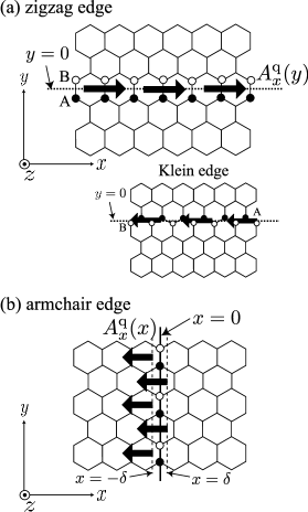
Figure 2: (a) The bonds on the dotted line at $y=0$ are cut to introduce the zigzag edge (Klein edge). The cutting is represented as a deformation-induced gauge field ${\bf A}^{\rm q}({\bf r})=(A_{x}^{\rm q}(y),0)$. (b) The deformation-induced gauge field for the armchair edge is given by ${\bf A}^{\rm q}({\bf r})=(A_{x}^{\rm q}(x),0)$.

The armchair edge can be introduced by cutting the bonds located on $x=\pm\delta$, as shown in Fig. 2(b). By setting $\delta\gamma_{0,1}({\bf r})=0$, $\delta\gamma_{0,2}({\bf r})|_{x=-\delta}=\gamma_{0}$ and $\delta\gamma_{0,3}({\bf r})|_{x=\delta}=\gamma_{0}$ in Eq. (6), the deformation-induced gauge field for the armchair edge is written as ${\bf A}^{\rm q}({\bf r})=(A_{x}^{\rm q}(x),0)$ with the limit of $\delta\to 0$. Due to translational symmetry along the $y$-axis, $\hat{p}_{y}$ is replaced to $p_{y}$ in Eq. (5). Thus, the Hamiltonian is given by

$$v_{\rm F}\begin{pmatrix}\sigma_{x}(\hat{p}_{x}+A_{x}^{\rm q}(x))+\sigma_{y}p_{y}&\phi^{\rm q}(x)\sigma_{x}\cr\phi^{\rm q}(x)^{*}\sigma_{x}&-\sigma_{x}(\hat{p}_{x}-A_{x}^{\rm q}(x))+\sigma_{y}p_{y}\end{pmatrix},$$

with $\phi^{\rm q}(x)=A^{\rm q}_{x}(x)e^{-2ik_{\rm F}x}$. This Hamiltonian can be reduced further by means of a gauge symmetry in the following manner. Since $A_{x}^{\rm q}(x)$ does not depend on $y$, it can be represented in terms of a scalar function $\varphi(x)$, as $A_{x}^{\rm q}(x)=\partial_{x}\varphi(x)$. Using the gauge transformation: $\Psi_{\rm K}(x)\to e^{-i\varphi(x)}\Psi_{\rm K}(x)$ and $\Psi_{\rm K^{\prime}}(x)\to e^{i\varphi(x)}\Psi_{\rm K^{\prime}}(x)$, $A_{x}^{\rm q}(x)$ can be erased from the Hamiltonian for each valley. However, note that as a result of this gauge transformation, $\phi^{\rm q}(x)$ must be changed into $e^{2i\varphi(x)}\phi^{\rm q}(x)$. To minimize notation, let us use $\phi^{\rm q}(x)$ to denote this gauge transformed field, so that $\phi^{\rm q}(x)\equiv A^{\rm q}_{x}(x)e^{2i[\varphi(x)-k_{\rm F}x]}$. The Hamiltonian for the armchair edge is then written as

$$H(x)=v_{\rm F}\begin{pmatrix}\sigma_{x}\hat{p}_{x}+\sigma_{y}p_{y}&\phi^{\rm q}(x)\sigma_{x}\cr\phi^{\rm q}(x)^{*}\sigma_{x}&-\sigma_{x}\hat{p}_{x}+\sigma_{y}p_{y}\end{pmatrix}.$$ (9)

This will be solved in Sec. V. Note that by introducing $\tau_{\alpha}$ ($\alpha=1,2,3$) matrices defined by

$$\tau_{1}=\begin{pmatrix}0&I\cr I&0\end{pmatrix},\ \tau_{2}=\begin{pmatrix}0&-iI\cr iI&0\end{pmatrix},\ \tau_{3}=\begin{pmatrix}I&0\cr 0&-I\end{pmatrix},$$ (10)

the unperturbed Hamiltonian is represented in a compact fashion as $H_{0}({\bf r})=v_{\rm F}(\tau_{3}\sigma_{x}\hat{p}_{x}+\tau_{0}\sigma_{y}\hat{p}_{y})$, where $\tau_{0}$ is a $4\times 4$ identity matrix.

In Eqs. (6) and (7), we assume $|\delta\gamma_{0,a}({\bf r})|\ll\gamma_{0}$, and ignore the higher order term of $\delta\gamma_{0,a}({\bf r})$. As a result of this simplification, the relationship between ${\bf A}^{\rm q}({\bf r})$ and $\delta\gamma_{0,a}({\bf r})$ may deviate from Eq. (6) when $|\delta\gamma_{0,a}(\mathbf{r})|\approx\gamma_{0}$. However, note that the direction and not the strength of the ${\bf A}^{\rm q}({\bf r})$ field can be determined by Eq. (6), even for the case where $|\delta\gamma_{0,a}({\bf r})|\approx\gamma_{0}$. Consideration of this point is given in Appendix A.

IV Zigzag edge

The scattering problem for the zigzag edge is solved in this section. Standing wave solutions are constructed in Sec. IV.1, and the properties of the solutions are examined in detail. Localized edge states are constructed in Sec. IV.2. The behavior of the standing wave in the presence of a mass term and an external magnetic field is examined in Secs. IV.3 and IV.4, respectively. The local density of states near the zigzag edge is calculated analytically in Sec. IV.5.

IV.1 Standing Waves

To begin with, solutions are constructed for the case of $A_{x}^{\rm q}(y)=0$ in Eq. (8). Let $\Phi(y)$ be the eigenstate of the unperturbed Hamiltonian $H_{\rm K}^{0}(y)=v_{\rm F}\left(\sigma_{x}p_{x}+\sigma_{y}\hat{p}_{y}\right)$. $H_{\rm K}^{0}(y)$ satisfies $\sigma_{x}H_{\rm K}^{0}(-y)\sigma_{x}=H_{\rm K}^{0}(y)$; therefore, a general solution may be constructed from the basis function $\Phi(y)$ to satisfy the constraint equation,

$$\Phi(-y)=e^{-ig}\sigma_{x}\Phi(y),$$ (11)

where $g$ is a real number phase. The phase $g$ can not be an arbitrary value. The successive operation of Eq. (11) on $\Phi(-y)$ gives $\Phi(-(-y))=e^{-2ig}\sigma_{x}^{2}\Phi(y)$, and hence $g$ should be $0$ or $\pi$. Note that a set of functions satisfying Eq. (11) is useful for construction of solutions in the case $A_{x}^{\rm q}(y)\neq 0$, because $H_{\rm K}(y)$ also satisfies $\sigma_{x}H_{\rm K}(-y)\sigma_{x}=H_{\rm K}(y)$. This constraint comes from the inversion symmetry of the gauge field with respect to $y=0$, $A_{x}^{\rm q}(-y)=A_{x}^{\rm q}(y)$.

From Eq. (11), we have $\Phi_{\rm B}(y)=e^{ig}\Phi_{\rm A}(-y)$. Thus, $\Phi(y)$ can be rewritten as

$$\Phi(y)=\begin{pmatrix}\Phi_{\rm A}(y)\cr\Phi_{\rm B}(y)\end{pmatrix}=\begin{pmatrix}\Phi_{\rm A}(y)\cr e^{ig}\Phi_{\rm A}(-y)\end{pmatrix}.$$ (12)

By substituting Eq. (12) into $H_{\rm K}^{0}(y)\Phi(y)=E\Phi(y)$, we obtain simultaneous differential equations:

$$\begin{split}&\frac{E}{v_{\rm F}}\Phi_{s}(y)=+p_{x}\Phi_{s}(y)+\hbar\frac{d}{dy}\Phi_{a}(y),\\ &\frac{E}{v_{\rm F}}\Phi_{a}(y)=-p_{x}\Phi_{a}(y)-\hbar\frac{d}{dy}\Phi_{s}(y),\end{split}$$ (13)

where $\Phi_{s}(y)$ and $\Phi_{a}(y)$ are defined as

$$\begin{split}&\Phi_{s}(y)\equiv e^{-i\frac{g}{2}}\Phi_{\rm A}(y)+e^{+i\frac{g}{2}}\Phi_{\rm A}(-y),\\ &\Phi_{a}(y)\equiv e^{-i\frac{g}{2}}\Phi_{\rm A}(y)-e^{+i\frac{g}{2}}\Phi_{\rm A}(-y).\end{split}$$ (14)

For the case $g=0$, Eq. (14) implies that $\Phi_{s}(y)$ is an even function [$\Phi_{s}(y)=\Phi_{s}(-y)$], while $\Phi_{a}(y)$ is an odd function [$\Phi_{a}(y)=-\Phi_{a}(-y)$]. Thus, they can be parameterized as follows:

$$\begin{split}&\Phi_{s}(y)=S\cos(k_{y}y),\\ &\Phi_{a}(y)=A\sin(k_{y}y),\end{split}$$ (15)

where the parameters $S$ and $A$ can be determined from Eq. (13). By substituting Eq. (15) into Eq. (13), we obtain the secular equation

$$\begin{pmatrix}\frac{E}{\hbar v_{\rm F}}-k_{x}&-k_{y}\cr-k_{y}&\frac{E}{\hbar v_{\rm F}}+k_{x}\end{pmatrix}\begin{pmatrix}S\cr A\end{pmatrix}=0.$$ (16)

The solution of this secular equation satisfies

$$\begin{split}&E^{2}=(\hbar v_{F})^{2}(k_{x}^{2}+k_{y}^{2}),\\ &A=\frac{k_{y}}{\frac{E}{\hbar v_{\rm F}}+k_{x}}S.\end{split}$$ (17)

Let $\theta({\bf k})$ be the polar angle between vector ${\bf k}$ and the $k_{x}$-axis. Then, $k_{x}=k\cos\theta({\bf k})$ and $k_{y}=k\sin\theta({\bf k})$ where $k=|{\bf k}|$, and the second equation of Eq. (17) can be rewritten as $A=S\tan\left[\theta({\bf k})/2\right]$ for the eigenstate with positive energy $E=\hbar v_{\rm F}k$. Assuming that $S=\cos\left[\theta({\bf k})/2\right]$, we have $A=\sin\left[\theta({\bf k})/2\right]$. Substituting these into Eq. (15) gives

$$\begin{split}&\Phi_{s}(y)=\cos\left(\frac{\theta({\bf k})}{2}\right)\cos(k_{y}y),\\ &\Phi_{a}(y)=\sin\left(\frac{\theta({\bf k})}{2}\right)\sin(k_{y}y).\end{split}$$ (18)

Then, Eq. (18) is substituted into Eq. (14) with $g=0$ to give

$$\Phi^{0}(y)=\begin{pmatrix}\cos\left(k_{y}y-\frac{\theta({\bf k})}{2}\right)\cr\cos\left(k_{y}y+\frac{\theta({\bf k})}{2}\right)\end{pmatrix}.$$ (19)

Similarly, for the case where $g=\pi$, we have

$$\Phi^{\pi}(y)=\begin{pmatrix}\sin\left(k_{y}y-\frac{\theta({\bf k})}{2}\right)\cr\sin\left(k_{y}y+\frac{\theta({\bf k})}{2}\right)\end{pmatrix}.$$ (20)

The energies of the eigenstates $\Phi^{0}(y)$ and $\Phi^{\pi}(y)$ are equal, and therefore a general solution can be expressed as a superposition of the degenerate eigenstates, as

$$\Phi^{f}(y) \equiv\sin(f)\Phi^{0}(y)+\cos(f)\Phi^{\pi}(y)$$

$$=\begin{pmatrix}\sin\left(k_{y}y-\theta({\bf k})/2+f\right)\cr\sin\left(k_{y}y+\theta({\bf k})/2+f\right)\end{pmatrix},$$ (21)

where $f$ is a real number. The value of $f$ is determined as follows.

The Hamiltonian, $H_{\rm K}(y)=H_{\rm K}^{0}(y)+v_{\rm F}\sigma_{x}A^{\rm q}_{x}(y)$, is identical to the unperturbed Hamiltonian $H_{\rm K}^{0}(y)$ for $y$ to satisfy $|y|\geq\xi_{g}$, so that $\Phi^{f}(y)$ satisfies the eigenequation $H_{\rm K}(y)\Phi^{f}(y)=E\Phi^{f}(y)$ for $|y|\geq\xi_{g}$. We need to solve $H_{\rm K}(y)\Psi_{\rm K}(y)=E\Psi_{\rm K}(y)$ locally for $|y|<\xi_{g}$. By parameterizing the eigenstate of $H_{\rm K}(y)$ as $\Psi_{\rm K}(y)=N(y)\Phi^{f}(y)$, we obtain the constraint equation for $N(y)$ and $\Phi^{f}(y)$ as

$$\left\{\sigma_{y}[\hat{p}_{y}N(y)]+\sigma_{x}A_{x}^{\rm q}(y)N(y)\right\}\Phi^{f}(y)=0.$$ (22)

To obtain Eq. (22) we must place $\Psi_{\rm K}(y)=N(y)\Phi^{f}(y)$ to $H_{\rm K}(y)\Psi_{\rm K}(y)=E\Psi_{\rm K}(y)$, and use $H_{\rm K}^{0}(y)\Phi^{f}(y)=E\Phi^{f}(y)$. Here, we have assumed that the energy eigenvalues of the standing wave $\Psi_{\rm K}(y)$ and of $\Phi^{f}(y)$ are the same. This assumption is valid for the standing wave, because the energy eigenvalue is determined by the bulk Hamiltonian $H_{\rm K}^{0}(y)$ and the energy does not change through elastic scattering. However, note that this assumption is not valid for the edge states, which $H_{\rm K}(y)\Psi_{\rm K}(y)=E\Psi_{\rm K}(y)$ must be solved directly (see Sec. IV.2 for more details). Now, Eq. (22) is equivalent to the two successive equations:

$$\begin{split}&\left(A_{x}^{\rm q}(y)N(y)-\hbar\frac{dN(y)}{dy}\right)\Phi^{f}_{\rm B}(y)=0,\\ &\left(A_{x}^{\rm q}(y)N(y)+\hbar\frac{dN(y)}{dy}\right)\Phi^{f}_{\rm A}(y)=0.\end{split}$$ (23)

The following two cases can be considered for this successive equation. One case is that the solution satisfies

$$\begin{split}&A_{x}^{\rm q}(y)N(y)+\hbar\frac{dN(y)}{dy}=0,\\ &\Phi^{f}_{\rm B}(y)=0,\end{split}\ \ \ (|y|\leq\xi_{g}).$$ (24)

The first (second) equation of Eq. (24) ensures the second (first) equation of Eq. (23). The other case is that the solution satisfies

$$\begin{split}&A_{x}^{\rm q}(y)N(y)-\hbar\frac{dN(y)}{dy}=0,\\ &\Phi^{f}_{\rm A}(y)=0,\end{split}\ \ \ (|y|\leq\xi_{g}).$$ (25)

The two conditions, Eqs. (24) and (25), correspond to the standing wave in the upper semi-infinite graphene plane for $y>0$ and that in the lower plane for $y<0$ in the limit of $\xi_{g}=0$, as shown in the following.

For the case of Eq. (24), the first equation is integrated with respect to $y$, to obtain

$$N(-\xi_{g})=N(\xi_{g})\exp\left(\frac{1}{\hbar}\int_{-\xi_{g}}^{\xi_{g}}A_{x}^{\rm q}(y)dy\right).$$ (26)

Hence, when $(1/\hbar)\int_{-\xi_{g}}^{\xi_{g}}A_{x}^{\rm q}(y)dy\gg 0$, $N(\xi_{g})$ is negligible compared with $N(-\xi_{g})$, and therefore the standing wave appears only for $y<0$. In contrast, when $(1/\hbar)\int_{-\xi_{g}}^{\xi_{g}}A_{x}^{\rm q}(y)dy\ll 0$, the standing wave appears only for $y>0$. The other condition in Eq. (24) holds for the limit of $\xi_{g}\to 0$ by setting $f=-\theta({\bf k})/2$ in Eq. (21), because

$$\lim_{y\to 0}\Phi^{f=-\theta({\bf k})/2}_{\rm B}(y)=0.$$ (27)

This condition leads to $\Psi_{{\rm K},{\rm B}}(0)=0$, which represents the boundary conditions for the zigzag and Klein edges shown in Fig. 2(a). Thus, Eq. (24) covers two situations, depending on the direction of the gauge field; $A_{x}^{\rm q}(y)\gg 0$ or $A_{x}^{\rm q}(y)\ll 0$. That is, when $A_{x}^{\rm q}(y)\gg 0$, Eq. (24) corresponds to the upper semi-infinite graphene plane with the zigzag edge, while when $A_{x}^{\rm q}(y)\ll 0$, Eq. (24) corresponds to the lower semi-infinite graphene plane with the Klein edge. Similarly, when $A_{x}^{\rm q}(y)\gg 0$, Eq. (25) corresponds to the lower semi-infinite graphene plane with the zigzag edge, while when $A_{x}^{\rm q}(y)\ll 0$, Eq. (25) corresponds to the upper semi-infinite graphene plane with the Klein edge.

From Eq. (26), it follows that the gauge field for the edge should be large, $\left|(1/\hbar)\int_{-\xi_{g}}^{\xi_{g}}A_{x}^{\rm q}(y)dy\right|\gg 1$. In Ref. Sasaki et al., 2006, the following was obtained analytically

$$\frac{1}{\hbar}\int_{-\xi_{g}}^{\xi_{g}}A_{x}^{\rm q}(y)dy=-\ln(1-c),$$ (28)

where $c$ is the parameter that specifies the deformation as $\delta\gamma_{0,1}({\bf r})|_{y=0}=c\gamma_{0}$ [see Fig. 2]. The right-hand side gives logarithmic singularities for $c=1$ and $c=-\infty$. The limit $c\to 1$ corresponds to the zigzag edge, while the limit $c\to-\infty$ represents the Klein edge. Note that when $c\to-\infty$, the electron is unable to have a finite amplitude on the A and B atoms located at $y=0$, which effectively represents the Klein edge. Because of the singularity, $N(y)$ that satisfies Eq. (26) is similar to the step function; $N(y)=N\neq 0$ for $y<0$, and otherwise $N(y)=0$.

Now, by setting $f=-\theta({\bf k})/2$ in Eq. (21), the standing wave in the conduction band is expressed as

$$\Psi^{c}_{{\rm K},{\bf k}}({\bf r})=\frac{e^{ik_{x}x}}{\sqrt{L_{x}}}N(y)\begin{pmatrix}\sin\left(k_{y}y-\theta({\bf k})\right)\cr\sin\left(k_{y}y\right)\end{pmatrix},$$ (29)

where the plane wave parallel to the edge with the length $L_{x}$ is included. The standing wave in the valence band is obtained by using the particle-hole symmetry of the Hamiltonian, $\sigma_{z}H_{\rm K}(y)\sigma_{z}=-H_{\rm K}(y)$, as $\Psi^{v}_{{\rm K},{\bf k}}(y)=\sigma_{z}\Psi^{c}_{{\rm K},{\bf k}}(y)$:

$$\Psi^{v}_{{\rm K},{\bf k}}({\bf r})=\frac{e^{ik_{x}x}}{\sqrt{L_{x}}}N(y)\begin{pmatrix}\sin\left(k_{y}y-\theta({\bf k})\right)\cr-\sin\left(k_{y}y\right)\end{pmatrix}.$$ (30)

Here, we consider the pseudospin of the standing wave. The pseudospin for an eigenstate $\Psi(y)$ is defined by the expected value of the Pauli matrices as $\langle\sigma_{i}\rangle\equiv\int\sigma_{i}(y)dy$ ($i=x,y,z$), where $\sigma_{i}(y)$ is a pseudospin density defined by $\sigma_{i}(y)\equiv\Psi^{\dagger}(y)\sigma_{i}\Psi(y)$. Note that the $y$-component of the pseudospin is proportional to the imaginary part of the Bloch function, such as $\sigma_{y}(y)\propto{\rm Im}[\Psi_{\rm A}^{*}\Psi_{\rm B}]$. The Bloch function of the standing wave is real, so that the $y$-component of the pseudospin for the standing wave vanishes, that is, $\langle\sigma_{y}\rangle=0$. Note also that $\langle\sigma_{y}\rangle=0$ means that the current normal to the zigzag edge vanishes. It is interesting to note that $\langle\sigma_{y}\rangle=0$ holds whenever $\Psi_{{\rm K},{\bf k},{\rm A}}(y)$ and $\Psi_{{\rm K},{\bf k},{\rm B}}(y)$ can be taken as real numbers. This indicates that the result $\langle\sigma_{y}\rangle=0$ is not sensitive to the value of $f$, but depends only on the fact that $\Phi^{f}$ does not have a relative phase between the two components. The condition of Eq. (27) means that the pseudospin density is locally polarized into the positive $z$-axis near the zigzag edge, that is, $\sigma_{z}(0)>0$ and $\sigma_{x}(0)=\sigma_{y}(0)=0$. Actually, by substituting $y\simeq 0$ into Eq. (29), the standing wave near the zigzag edge has amplitude only at A-atoms. This polarization of the pseudospin is consistent with the fact that the gauge field $A_{x}^{\rm q}(y)$ has a non-vanishing deformation-induced magnetic field,

$$B_{z}^{\rm q}({\bf r})\equiv\partial_{x}A_{y}^{\rm q}({\bf r})-\partial_{y}A_{x}^{\rm q}({\bf r}),$$ (31)

at the zigzag edge. The presence of the $B_{z}^{\rm q}(y)$ field at the zigzag edge causes local polarization of the standing wave pseudospin near the zigzag edge, similar to the polarization of a real spin by a magnetic field. We will show in Sec. IV.5 that this polarization of the pseudospin causes anomalous behavior to appear in the local density of states (LDOS) near the zigzag edge.

A zigzag nanoribbon is given by introducing another zigzag edge at $y=-L$, in addition to the zigzag edge at $y=0$. Suppose that the edge atoms at $y=-L$ are B-atoms, which imposes the boundary condition on the wave function at $y=-L$ as $\lim_{y=-L}\Psi_{{\rm K},{\bf k},{\rm A}}^{c}({\bf r})=0$. This leads to the constraint equation for $(k_{x},k_{y})$,

$$k_{y}L+\theta({\bf k})=n\pi,$$ (32)

where $n$ is an integer. It is noted that this equation reproduces

$$k_{y}=-k_{x}\tan(k_{y}L),$$ (33)

which was obtained by Brey and Fertig in Ref. Brey and Fertig, 2006 [the negative sign in front of $k_{x}$ is a matter of notation]. Note that $n$ should be a nonzero integer, because the equation does not possess a solution when $n=0$. For the case where the edge at $y=-L$ is the Klein edge, the boundary condition on the wave function at $y=-L$ becomes $\lim_{y=-L}\Psi_{{\rm K},{\bf k},{\rm B}}^{c}({\bf r})=0$. This leads to $k_{y}L=n\pi$, where $n$ is a positive integer.

IV.2 Edge States

In addition to the standing wave derived in the previous subsection, $H_{\rm K}(y)$ possesses localized edge states. Sasaki et al. (2006) Here, we show how to construct the edge states.

The following observation is useful in order to obtain the edge states. Instead of Eq. (15), we assume

$$\begin{split}&\Phi_{s}(y)=S\cosh(y/\xi),\\ &\Phi_{a}(y)=A\sinh(y/\xi).\end{split}$$ (34)

By substituting Eq. (34) into Eq. (13), the secular equation is obtained:

$$\begin{pmatrix}\frac{E}{\hbar v_{\rm F}}-k_{x}&-\xi^{-1}\cr+\xi^{-1}&\frac{E}{\hbar v_{\rm F}}+k_{x}\end{pmatrix}\begin{pmatrix}S\cr A\end{pmatrix}=0.$$ (35)

The solution of this secular equation satisfies

$$\begin{split}&E^{2}=(\hbar v_{F})^{2}\left(k_{x}^{2}-\xi^{-2}\right),\\ &A=-\frac{\xi^{-1}}{\frac{E}{\hbar v_{\rm F}}+k_{x}}S.\end{split}$$ (36)

By introducing the $\phi$ variable, which satisfies

$$\xi^{-1}=-k_{x}\tanh\phi,$$ (37)

we have $E^{2}/(\hbar v_{F})^{2}=k_{x}^{2}/\cosh^{2}\phi$. For the case

$$\frac{E}{\hbar v_{\rm F}}=\frac{k_{x}}{\cosh\phi},$$ (38)

we have $A/S=\tanh(\phi/2)$. By inserting this into Eq. (34) and setting $S=\cosh(\phi/2)$, we obtain

$$\begin{split}&\Phi_{s}(y)=\cosh\left(\frac{\phi}{2}\right)\cosh\left(\frac{y}{\xi}\right),\\ &\Phi_{a}(y)=\sinh\left(\frac{\phi}{2}\right)\sinh\left(\frac{y}{\xi}\right).\end{split}$$ (39)

By substituting Eq. (39) into Eq. (14) with $g=0$, we have

$$\Phi^{0}(y)=\begin{pmatrix}\cosh\left(\frac{y}{\xi}+\frac{\phi}{2}\right)\cr\cosh\left(\frac{y}{\xi}-\frac{\phi}{2}\right)\end{pmatrix}.$$ (40)

Similarly, for the case $g=\pi$, we have

$$\Phi^{\pi}(y)=\begin{pmatrix}\sinh\left(\frac{y}{\xi}+\frac{\phi}{2}\right)\cr\sinh\left(\frac{y}{\xi}-\frac{\phi}{2}\right)\end{pmatrix}.$$ (41)

The energies of $\Phi^{\pi}(y)$ and $\Phi^{0}(y)$ are equal; therefore, the basis function may be chosen as

$$\begin{split}&\Phi^{+}(y)\equiv\Phi^{0}(y)+\Phi^{\pi}(y)=e^{+\frac{y}{\xi}}\begin{pmatrix}e^{+\phi/2}\cr e^{-\phi/2}\end{pmatrix},\\ &\Phi^{-}(y)\equiv\Phi^{0}(y)-\Phi^{\pi}(y)=e^{-\frac{y}{\xi}}\begin{pmatrix}e^{-\phi/2}\cr e^{+\phi/2}\end{pmatrix}.\end{split}$$ (42)

The functions $\Phi^{+}(y)$ and $\Phi^{-}(y)$ are exponentially increasing and decreasing functions of $y$, respectively. Thus, neither $\Phi^{+}(y)$ nor $\Phi^{-}(y)$ is a normalized wave function all over the space, $y\in(-\infty,\infty)$. However, note that $\Phi^{+}(y)$ and $\Phi^{-}(y)$ can be normalizable wave functions for $y<0$ and $y>0$, respectively. We also note that the pseudospin of $\Phi^{+}(y)$ is given by $\langle\sigma_{z}\rangle=\tanh\phi$, while that of $\Phi^{-}(y)$ is $\langle\sigma_{z}\rangle=-\tanh\phi$.

From the above observation, we parameterized the localized eigenstate as

$$\Psi_{\rm K}(y)=Ne^{-\frac{|y|}{\xi}}\begin{pmatrix}e^{+g(y)}\cr e^{-g(y)}\end{pmatrix},$$ (43)

where $N$ is a normalization constant, and the modulation of the pseudospin is represented by a function $g(y)$. Substituting Eq. (43) into $H_{\rm K}(y)\Psi_{\rm K}(y)=E\Psi_{\rm K}(y)$ gives simultaneous differential equations for $g(y)$,

$$\begin{split}&p_{x}+A^{\rm q}_{x}(y)+\hbar\frac{d}{dy}\left(\frac{|y|}{\xi}+g(y)\right)=\frac{E}{v_{F}}e^{+2g(y)},\\ &p_{x}+A^{\rm q}_{x}(y)-\hbar\frac{d}{dy}\left(\frac{|y|}{\xi}-g(y))\right)=\frac{E}{v_{F}}e^{-2g(y)}.\end{split}$$ (44)

By summing and subtracting both sides of Eq. (44), the energy eigenequation can be rewritten as

$$\begin{split}&p_{x}+A^{\rm q}_{x}(y)+\hbar\frac{dg(y)}{dy}=\frac{E}{v_{F}}\cosh(2g(y)),\\ &\hbar\frac{d}{dy}\left(\frac{|y|}{\xi}\right)=\frac{E}{v_{F}}\sinh(2g(y)).\end{split}$$ (45)

The solution of the second equation is given by

$$g(y)=\begin{cases}\displaystyle-\frac{1}{2}\sinh^{-1}\left(\frac{\hbar v_{F}}{\xi E}\right)&(y<0),\\ \displaystyle+\frac{1}{2}\sinh^{-1}\left(\frac{\hbar v_{F}}{\xi E}\right)&(y>0).\end{cases}$$ (46)

The sign of $g(y)$ changes across the zigzag edge, and this sign change indicates that the $z$-component of the pseudospin flips at the edge. The flip is induced by the gauge field $A^{\rm q}_{x}(y)$. To represent this, we integrate the first equation of Eq. (45) from $y=-\xi_{g}$ to $\xi_{g}$, and acquire

$$-\int_{-\xi_{g}}^{\xi_{g}}\frac{dg(y)}{dy}dy=\frac{1}{\hbar}\int_{-\xi_{g}}^{\xi_{g}}A^{\rm q}_{x}(y)dy.$$ (47)

We have neglected other terms, because they are proportional to $\xi_{g}$ and become zero in the limit of $\xi_{g}=0$. By substituting Eq. (46) into Eq. (47), we find

$$-\sinh^{-1}\left(\frac{\hbar v_{F}}{\xi E}\right)=\frac{1}{\hbar}\int_{-\xi_{g}}^{\xi_{g}}A^{\rm q}_{x}(y)dy.$$ (48)

Hence, Eq. (46) becomes

$$g(y)=\begin{cases}\displaystyle+\frac{1}{2}\left(\frac{1}{\hbar}\int_{-\xi_{g}}^{\xi_{g}}A^{\rm q}_{x}(y)dy\right)&(y<0),\\ \displaystyle-\frac{1}{2}\left(\frac{1}{\hbar}\int_{-\xi_{g}}^{\xi_{g}}A^{\rm q}_{x}(y)dy\right)&(y>0).\end{cases}$$ (49)

Having described the wave function of the localized state, let us now calculate $E$ and $\xi$. To this end, we use the first equation of Eq. (45) for $|y|\geq\xi_{g}$ and obtain

$$\frac{E}{v_{F}}=\frac{p_{x}}{\cosh\left(\displaystyle\frac{1}{\hbar}\int_{-\xi_{g}}^{\xi_{g}}A^{\rm q}_{x}(y)dy\right)}.$$ (50)

Moreover, using Eq.(48), we find

$$\frac{1}{\xi}=-k_{x}\tanh\left(\displaystyle\frac{1}{\hbar}\int_{-\xi_{g}}^{\xi_{g}}A^{\rm q}_{x}(y)dy\right).$$ (51)

In addition to this localized state, there is another localized state for the same $k_{x}$ with the same $\xi$, but with the opposite sign of $E$. This results from the particle-hole symmetry of the Hamiltonian, and the wave function is given by $\sigma_{z}\Psi_{\rm K}(y)$.

In the following, we will show that the solutions can reproduce all the properties of the edge states known in the tight-binding lattice (TB) model, Tanaka et al. (1987); Fujita et al. (1996); Nakada et al. (1996) such as the asymmetric energy band structure with respect to the K (K^′) point, the flat energy band, and the pseudospin structure.

The asymmetric energy band structure with respect to the K (K^′) point originates from the normalization condition of the wave function, which requires that $\xi$ should be positive. This requirement restricts the value of $k_{x}$ in Eq. (51). When $A^{\rm q}_{x}(y)$ is positive, Eq. (51) indicates that the localized states appear only at $k_{x}<0$ around the K point. This is the reason why the localized states appear in the energy spectrum only at one side around the K point. A similar argument can be used for the K^′ point, which concludes that the localized state appears at $k_{x}>0$ around the K^′ point. The Hamiltonian around the K^′ point is expressed by

$$H_{\rm K^{\prime}}({\bf r})=v_{F}\mbox{\boldmath$\sigma$}^{\prime}\cdot(\hat{\bf p}-{\bf A}^{\rm q}({\bf r})).$$ (52)

Therefore, we obtain different signs in front of $\bf{A}^{\rm q}(\bf{r})$ in $H_{\rm K}(y)$ and Eq. (52), which causes the negative sign in front of the right-hand side of Eq. (51) to disappear for the K^′ point. Thus, when $A^{\rm q}_{x}(y)$ is negative (Klein edges), edge states appear on the opposite side; $k_{x}>0$ around the K point and $k_{x}<0$ around the K^′ point. Calculations on the TB model with Klein edges also agree with the results obtained here.

A singularity of the gauge field, $|A^{\rm q}_{x}(y)|\to\infty$, is the origin of the flat energy dispersion and the pseudospin polarization of the edge states. When $(1/\hbar)\int_{-\xi_{g}}^{\xi_{g}}A_{x}(y)dy\to\infty$, $E$ in Eq. (50) becomes zero. The zero energy eigenvalue between the K and K^′ points in the band structure corresponds to the flat energy band of the edge state. Fujita et al. (1996) Moreover, from Eq. (49), $g(y)\to\infty$ for $y<0$ and $g(y)\to-\infty$ for $y>0$ are obtained. In this case, the localized state is a pseudospin-up state $\Psi_{\rm K}({\bf r})\propto{}^{t}(1,0)$ for $y<0$ and a pseudospin-down state $\Psi_{\rm K}({\bf r})\propto{}^{t}(0,1)$ for $y>0$. Hence, a singular gauge field at the zigzag edge causes polarization of the pseudospin of the localized states. Polarization of the pseudospin means that the wave function has amplitude only at the A (or B) atom, so that this result agrees with the result from the TB model for the edge state. Fujita et al. (1996) Comparing Eqs. (51) and (50) with Eqs. (37) and (38), the relation between the variable $\phi$ and the field $A_{x}^{\rm q}(y)$ is observed as $\phi=(1/\hbar)\int_{-\xi_{g}}^{\xi_{g}}A_{x}^{\rm q}(y)dy$.

Here, we note that $N$ in Eq. (43) is not a function of $y$, but is a constant for $y\in(-\infty,\infty)$. Therefore, the edge states appear on both sides of the zigzag edge, $y>0$ and $y<0$, while the standing waves appear on only one side of the edge under the limit $(1/\hbar)\int_{-\xi_{g}}^{\xi_{g}}A_{x}^{\rm q}(y)dy\to\pm\infty$. With this limit, the edge states can be confined to one side of the edge, because the energy of the localized state becomes $E=0$, and therefore, the superposition of an edge state, $\Psi_{\rm K}(y)$, and its electron-hole pair state, $\sigma_{z}\Psi_{\rm K}(y)$, is a solution. It is easy to see that $\Psi_{\rm K}(y)+\sigma_{z}\Psi_{\rm K}(y)$ has amplitude only for $y<0$, while $\Psi_{\rm K}(y)-\sigma_{z}\Phi_{\rm K}(y)$ has amplitude only for $y>0$. The wave function of the edge state for $y<0$ is then given by

$$\Psi_{{\rm K},k_{x}<0}({\bf r})=\frac{e^{ik_{x}x}}{\sqrt{L_{x}}}\sqrt{2|k_{x}|}e^{k_{x}|y|}\begin{pmatrix}1\cr 0\end{pmatrix},$$ (53)

where the normalization constant has been fixed, $\sqrt{2|k_{x}|}$, by assuming that the system is a semi-infinite graphene plane. We note that the mass term, $m\sigma_{z}$, is proportional to the particle-hole symmetry operator, $\sigma_{z}$. Thus, the mass term automatically restricts the region where the edge states can appear ($y>0$ or $y<0$), and this is shown in Appendix B.

Finally, we consider the edge states in nanoribbons. Note first that the exact localization length for the case of a zigzag nanoribbon with width $L$ satisfies

$$\begin{split}&\frac{1}{\xi}=-k_{x}\tanh\left(\frac{L}{\xi}\right),\\ &\left[\leftrightarrow-k_{x}L=(k_{x}\xi){\rm atanh}\left(\frac{1}{k_{x}\xi}\right)\right],\end{split}$$ (54)

which is obtained by analytical continuation $k_{y}=i/\xi$ for Eq. (33). Comparing this equation with Eq. (51) shows that the large value of the gauge field in Eq. (51) corresponds to the case of $L/\xi\gg 1$ in Eq. (54). This is consistent with having solved the Hamiltonian locally near the edge, in which it was implicitly assumed that the condition $L/\xi\gg 1$ is satisfied. Except the edge states whose localization length is in the order of $L$, Eqs. (51) and (54) give almost identical values of $\xi\simeq-k^{-1}_{x}$, which justifies the description using the gauge field. Note also that the condition $L/\xi\gg 1$ also represents the condition $k_{x}L\ll-1$, which is clear from the second equation in Eq. (54). To solve the Hamiltonian for the edge states with $\xi={\cal O}(L)$, Eq. (45) must be solved globally, for example, on a circle, which is a challenging issue.

IV.3 Mass Term

Let us reconsider the scattering problem for the case where the Hamiltonian includes a mass term. The total Hamiltonian is given by $H^{m}_{\rm K}(y)\equiv H_{\rm K}(y)+m\sigma_{z}$, where the mass, $m$, is a constant over the space $y\in(-\infty,+\infty)$. The solutions of $H^{m}_{\rm K}(y)$ can be constructed from the solutions of $H_{\rm K}(y)$ as follows.

For $H_{\rm K}(y)$, the standing wave solutions, Eqs. (29) and (30), satisfy

$$\begin{split}&H_{\rm K}(y)\Psi^{c}_{{\rm K},{\bf k}}(y)=\hbar v_{\rm F}k\Psi^{c}_{{\rm K},{\bf k}}(y),\\ &H_{\rm K}(y)\Psi^{v}_{{\rm K},{\bf k}}(y)=-\hbar v_{\rm F}k\Psi^{v}_{{\rm K},{\bf k}}(y).\end{split}$$ (55)

For the mass term, because $\Psi^{v}_{{\rm K},{\bf k}}(y)=\sigma_{z}\Psi^{c}_{{\rm K},{\bf k}}(y)$, we obtain

$$\begin{split}&m\sigma_{z}\Psi^{c}_{{\rm K},{\bf k}}(y)=m\Psi^{v}_{{\rm K},{\bf k}}(y),\\ &m\sigma_{z}\Psi^{v}_{{\rm K},{\bf k}}(y)=m\Psi^{c}_{{\rm K},{\bf k}}(y).\end{split}$$ (56)

Thus, by changing the basis state from $|\Psi^{c}_{{\rm K},{\bf k}}\rangle$ and $|\Psi^{v}_{{\rm K},{\bf k}}\rangle$ into $|\Psi_{{\rm K},{\bf k},{\rm A}({\rm B})}\rangle$ $[\equiv(1/\sqrt{2})(|\Psi^{c}_{{\rm K},{\bf k}}\rangle\pm|\Psi^{v}_{{\rm K},{\bf k}}\rangle)]$, the Hamiltonian is represented as

$$H^{m}_{\rm K} \to\begin{pmatrix}\langle\Psi_{{\rm K},{\bf k},{\rm A}}|H^{m}_{\rm K}|\Psi_{{\rm K},{\bf k},{\rm A}}\rangle&\langle\Psi_{{\rm K},{\bf k},{\rm A}}|H^{m}_{\rm K}|\Psi_{{\rm K},{\bf k},{\rm B}}\rangle\cr\langle\Psi_{{\rm K},{\bf k},{\rm B}}|H^{m}_{\rm K}|\Psi_{{\rm K},{\bf k},{\rm A}}\rangle&\langle\Psi_{{\rm K},{\bf k},{\rm B}}|H^{m}_{\rm K}|\Psi_{{\rm K},{\bf k},{\rm B}}\rangle\end{pmatrix}$$

$$=\begin{pmatrix}m&\hbar v_{\rm F}k\cr\hbar v_{\rm F}k&-m\end{pmatrix}.$$ (57)

Here, the angle $\phi_{k}$ is defined as

$$\cos\phi_{k}\equiv\frac{m}{E_{k}},\ \ \sin\phi_{k}\equiv\frac{\hbar v_{\rm F}k}{E_{k}},$$ (58)

where $E_{k}\equiv\sqrt{m^{2}+(\hbar v_{\rm F}k)^{2}}$. The normalized eigenvectors of the matrix in Eq. (57) are then

$$\begin{pmatrix}\cos\frac{\phi_{k}}{2}\cr\sin\frac{\phi_{k}}{2}\end{pmatrix}\ \ {\rm and}\ \ \begin{pmatrix}-\sin\frac{\phi_{k}}{2}\cr\cos\frac{\phi_{k}}{2}\end{pmatrix}$$ (59)

for the $E_{k}$ and $-E_{k}$ eigenvalues, respectively. $\Psi_{{\rm K},{\bf k},{\rm A}}(y)=\sqrt{2}N(y)\sin(k_{y}y-\theta({\bf k}))$ and $\Psi_{{\rm K},{\bf k},{\rm B}}(y)=\sqrt{2}N(y)\sin(k_{y}y)$ are obtained from Eqs. (29) and (30); therefore, the standing wave near the zigzag edge is given by

$$\begin{split}&\Psi^{m,c}_{{\rm K},{\bf k}}(y)=\sqrt{2}N(y)\begin{pmatrix}\cos\left(\frac{\phi_{k}}{2}\right)\sin\left(k_{y}y-\theta({\bf k})\right)\cr\sin\left(\frac{\phi_{k}}{2}\right)\sin\left(k_{y}y\right)\end{pmatrix},\\ &\Psi^{m,v}_{{\rm K},{\bf k}}(y)=\sqrt{2}N(y)\begin{pmatrix}-\sin\left(\frac{\phi_{k}}{2}\right)\sin\left(k_{y}y-\theta({\bf k})\right)\cr\cos\left(\frac{\phi_{k}}{2}\right)\sin\left(k_{y}y\right)\end{pmatrix},\end{split}$$ (60)

where we have omitted to write the plane wave parallel to the edge. The factors $\cos\left(\phi_{k}/2\right)$ and $\sin\left(\phi_{k}/2\right)$ appear in a manner similar to the eigenvalue problem of the spin magnetic moment in a magnetic field.

IV.4 External Magnetic Field

In this subsection, solutions are constructed for a magnetic field applied perpendicular to the graphene plane. McClure (1956) A magnetic field $B$ can be represented by the electromagnetic gauge field as ${\bf A}(y)=(By,0)$. This gauge field is included in the Hamiltonian by substituting the momentum operator ${\bf{\hat{p}}}$ with ${\bf{\hat{p}}}-e{\bf A}$. For the case $A^{\rm q}_{x}(y)=0$, the eigenequation becomes

$$v_{\rm F}\left[\sigma_{x}(\hat{p}_{x}-eBy)+\sigma_{y}\hat{p}_{y}\right]\Phi({\bf r})=E\Phi({\bf r}),$$ (61)

and the solutions are given by the Landau states, which are specified by an integer $n$ and a center coordinate $Y$ as

$$\Phi^{\rm LL}_{nY}({\bf r}) =C_{nY}e^{i\frac{Yx}{{\it l}^{2}}}e^{-\frac{1}{2}\left(\frac{y-Y}{\it l}\right)^{2}}$$

$$\times\begin{pmatrix}{\rm sgn}(n)\sqrt{2|n|}H_{|n|-1}\left((y-Y)/{\it l}\right)\cr-H_{|n|}\left((y-Y)/{\it l}\right)\end{pmatrix},$$ (62)

where $C_{nY}$ is a normalization constant, ${\it l}=\sqrt{\hbar/eB}$, and $H_{n}(x)$ is a Hermite polynomial defined by $H_{n}(x)\equiv(-1)^{n}e^{x^{2}}(d/dx)^{n}e^{-x^{2}}$ ($n\geq 0$). The energy eigenvalue of $\Phi^{\rm LL}_{nY}({\bf r})$ is given by $E_{n}={\rm sgn}(n)\sqrt{2|n|}\hbar v_{\rm F}/{\it l}$.

A method similar to that in Sec. IV.1 is used to solve the scattering problem in the presence of a magnetic field. The energy eigenstate of $H_{\rm K}({\bf r})$ is parameterized as $\Psi_{\rm K}({\bf r})=N(y)\Phi^{\rm LL}_{nY}({\bf r})$. Substituting this into $H_{\rm K}({\bf r})\Psi_{\rm K}({\bf r})=E_{n}\Psi_{\rm K}({\bf r})$, and using $H^{0}_{\rm K}({\bf r})\Phi^{\rm LL}_{nY}({\bf r})=E_{n}\Phi^{\rm LL}_{nY}({\bf r})$, we obtain the constraint equation for $N(y)$ and $\Phi^{\rm LL}_{nY}({\bf r})$,

$$\left\{\sigma_{y}[\hat{p}_{y}N(y)]+\sigma_{x}A_{x}^{\rm q}(y)N(y)\right\}\Phi^{\rm LL}_{nY}({\bf r})=0.$$ (63)

Two cases can be considered as a solution for this successive equation [see Eqs. (24) and (25)]. Here, we choose the case where

$$\begin{split}&A_{x}^{\rm q}(y)N(y)+\hbar\frac{dN(y)}{dy}=0,\\ &\Phi^{\rm LL}_{nY,{\rm B}}({\bf r})=0,\end{split}\ \ \ (|y|\leq\xi_{g}).$$ (64)

From Eq. (62), the second equation leads to

$$C_{nY}e^{-\frac{1}{2}\left(\frac{Y}{\it l}\right)^{2}}H_{|n|}\left(-2Y/{\it l}\right)=0,$$ (65)

with the limit $\xi_{g}\to 0$ ($y\to 0$). The number of zeros of $H_{n}$ is $|n|$, so that there are $|n|$ solutions of Eq. (65), which are denoted as $Y_{i}$ ($i=0,\cdots,|n|$). The solutions can then be written as

$$\Psi_{{\rm K},nY_{i}}({\bf r})=N(y)\Phi^{\rm LL}_{nY_{i}}({\bf r}).$$ (66)

Note that $\Psi_{{\rm K},nY}({\bf r})$ with a large value of $Y$ that satisfies $Y\gg{\it l}$, can be an approximate solution, due to the exponential factor in Eq. (65). The solution with a large value of $Y$ represents the wave function in the bulk, and is not sensitive to the details of the edge. The solutions given in Eq. (66) concern the Landau states near the zigzag edge, and these are examined in the following.

For the case that $n$ is an odd integer, $Y=0$ satisfies Eq. (65), because $H_{n}(0)=0$. The wave function with $Y=0$ decays according to $\exp(-y^{2}/2{\it l}^{2})$, and the amplitude has a maximum at the zigzag edge. Note that the localization length is in the order of ${\it l}$ (${\it l}\simeq 25[{\rm nm}]/\sqrt{B[{\rm T}]}$), which is larger than the localization length of the edge state $\xi=-k_{x}^{-1}$ where $k_{x}^{-1}$ takes a value of the same order as the lattice constant.

The lowest Landau level ($n=0$) can not satisfy the condition of Eq. (65) because $H_{0}(-2Y/{\it l})=1$ and the amplitudes of B-atoms do not vanish at the edge. Thus, the lowest Landau level is absent for the K point. On the other hand, the lowest Landau level appears for the K^′ point. The Hamiltonian for the K^′ point is given by

$$H_{\rm K^{\prime}}({\bf r})=v_{\rm F}\left[-\sigma_{x}(\hat{p}_{x}-eA_{x}(y)-A^{\rm q}_{x}(y))+\sigma_{y}\hat{p}_{y}\right].$$ (67)

For the case of $A^{\rm q}_{x}(y)=0$, $H_{\rm K}({\bf r})$ and $H_{\rm K^{\prime}}({\bf r})$ are related as $H_{\rm K^{\prime}}({\bf r})=\sigma_{y}H_{\rm K}({\bf r})\sigma_{y}$, and therefore the solutions for the K^′ point are given by $\sigma_{y}\Phi^{\rm LL}_{nY^{\prime}}({\bf r})$. The constraint equation for the K^′ point is

$$\left\{\sigma_{y}[\hat{p}_{y}N(y)]+\sigma_{x}A_{x}^{\rm q}(y)N(y)\right\}\sigma_{y}\Phi^{\rm LL}_{nY^{\prime}}({\bf r})=0,$$ (68)

which reduces to the condition $\Phi^{\rm LL}_{nY^{\prime},{\rm A}}(y)=0$. The solution is then given by

$$\Psi_{{\rm K^{\prime}},nY^{\prime}_{j}}({\bf r})=N(y)\sigma_{y}\Phi^{\rm LL}_{nY^{\prime}_{j}}({\bf r}),$$ (69)

where $Y^{\prime}_{j}$ denotes the solution of the constraint equation,

$$C_{nY}e^{-\frac{1}{2}\left(\frac{Y}{{\it l}}\right)^{2}}\sqrt{2|n|}H_{|n|-1}\left(-Y/{\it l}\right)=0.$$ (70)

This condition is satisfied for $n=0$, so that the lowest Landau level appears for the K^′ point. There is no constraint for the value of $Y$. For the case of the first Landau levels ($n=\pm 1$), the Landau level for the K point appears, while that for the K^′ point disappears. Therefore, near the zigzag edge, the lowest and first Landau levels are not symmetric with respect to the K and K^′ points.

IV.5 Local Density of States

Several groups have conducted scanning tunneling spectroscopy (STS) measurements to determine the LDOS near the step edge of graphite. Klusek et al. (2000); Giunta and Kelty (2001); Kobayashi et al. (2005); Niimi et al. (2005) A peak structure in the LDOS due to the edge states has been extensively discussed by many authors. Here, we calculate the LDOS near the zigzag edge. We show that some characteristic features that originate from the pseudospin polarization, the edge states, and the mass appear in the LDOS.

Let us first review the LDOS for graphene without an edge. Assuming that electrons are non-interacting, the bulk LDOS is given by

$$\rho(E)=\frac{1}{2\pi}\frac{|E|}{(\hbar v_{\rm F})^{2}},$$ (71)

where $\rho(E)$ is proportional to $|E|$, which results from the Dirac cone spectrum. Note that the actual LDOS is given by $g_{s}g_{v}\rho(E)$, where $g_{s}=2$ ($g_{v}=2$) accounts for the spin (valley) degrees of freedom. Next, the LDOS near the zigzag edge is calculated using the solutions given in Eq. (60). The LDOS has the form,

$$\rho_{s}(E,y)=\frac{1}{2\pi}\frac{|E|}{(\hbar v_{\rm F})^{2}}R(E,y),$$ (72)

where $R(E,y)$ is defined as

$$R(E,y)\equiv\frac{1}{\pi}\int^{\pi}_{0}d\theta\Psi^{m}_{{\rm K},{\bf k}}(y)^{\dagger}\Psi^{m}_{{\rm K},{\bf k}}(y).$$ (73)

By performing the integral with respect to the angle $\theta$ in Eq. (73), we obtain an analytical result for $R(E,y)$ as

$$R(E,y)=\begin{cases}\displaystyle F\left(k|y|\right)+\frac{m}{|E|}G\left(k|y|\right)\ \ (E>0),\\ \displaystyle F\left(k|y|\right)-\frac{m}{|E|}G\left(k|y|\right)\ \ (E<0),\end{cases}$$ (74)

where $k$ is a function of $E$ according to $k=\sqrt{E^{2}-m^{2}}/(\hbar v_{\rm F})$, and the functions $F$ and $G$ are defined as

$$\begin{split}&F(k|y|)\equiv 1-\left\{\frac{J_{0}(2k|y|)+J_{2}(2k|y|)}{2}\right\},\\ &G(k|y|)\equiv\frac{J_{0}(2k|y|)-J_{2}(2k|y|)}{2}.\end{split}$$ (75)

Here, $J_{\nu}(x)$ is a Bessel function of order $\nu$.

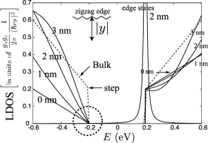
Figure 3: Positional dependence of the LDOS structure for the cases of $m=0.2$[eV]. The number located on each solid line represents the distance (corresponding to $|y|$ in the inset) from the zigzag edge. The LDOS at $E=-m$ vanishes near the zigzag edge, which is emphasized by the dashed circle. The dashed line denotes the LDOS in the bulk which is defined by the LDOS at $|y|\to\infty$. A peak structure due to the edge states is plotted for comparison. Note that there are several intrinsic perturbations Sasaki et al. (2009) that can change the position of the peak.

Because the case of $m=0$ has been considered elsewhere, Sasaki et al. (2010b) we consider the case $m\neq 0$ here. Eq. (71) holds for $|E|\geq|m|$. The bulk LDOS vanishes for the case $|E|<|m|$, as shown by the dashed line in Fig. 3. Note that the LDOS disappears suddenly at $E=\pm m$, and the bulk LDOS has a step like structure at $E=\pm|m|$. The bulk LDOS is symmetric with respect to $E=0$, even for the case $m\neq 0$. However, note that the LDOS near the edge is not symmetric for the case of $m\neq 0$, which is clear from the different signs in front of the function $G$ in Eq. (74). In Fig. 3, the LDOS are plotted at $|y|=0$, 1, 2, and 3 [nm] for the case of $m=0.2$ eV. Note that for the case $m=-0.2$ eV, the corresponding LDOS curve is given by interchanging the conduction and valence bands in Fig. 3.

The asymmetry in the LDOS near the edge appears at the following points. First, a step structure appears only at $E=0.2$ eV. At $E=-0.2$ eV, the LDOS vanishes, and the step structure is absent, as indicated by the dashed circle in Fig. 3. The absence of the LDOS at $E=-0.2$ eV can be explained by the zigzag edge consisting of A-atoms makes the standing wave polarized into A-atoms near the zigzag edge. However, eigenstates with energy $E=-m$ should be polarized into B-atoms by the factors in Eq. (59), and the amplitude of A-atoms are strongly suppressed by the mass term. Therefore, electrons with energy $E=-m$ can not approach the zigzag edge, and therefore the LDOS disappears. Secondly, the LDOS peak of the edge states appears only at $E=0.2$ eV. This is a straightforward consequence of the edge state amplitude appearing only for A-atoms. The absence of the LDOS at $E=-m$ and the presence of the peak at $E=m$ due to the edge states occurs at different sides of the band edge. To plot the LDOS of the edge states in Fig. 3, we have used

$$\rho_{e}(E,y)=\frac{1}{2\pi^{2}}\frac{2\delta}{(E-m)^{2}+\delta^{2}}\frac{1}{4y^{2}},$$ (76)

where $\delta$ is a phenomenological parameter that represents the energy uncertainty of the edge states, for which we assume $\delta=10$ meV. This result has been derived in Ref. Sasaki et al., 2010b for the case of $m=0$. Note that $\rho_{e}(E,y)$ decreases as $\sim y^{-2}$, which is a slowly decreasing function compared with the exponential decay wave function of the edge state.

V Armchair edge

In this section, the scattering problem for the armchair edge is solved using a method similar to that used in Sec. IV. The standing wave shows that the pseudospin does not change its direction through the reflection at the armchair edge.

V.1 Standing Waves

Solutions for the case of $\phi^{\rm q}(x)=0$ in Eq. (9) are constructed first, and then used as the basis functions to construct the standing wave near the armchair edge. Let $\Phi(x)$ represent the solution of the unperturbed Hamiltonian, $H_{0}(x)=v_{\rm F}(\tau_{3}\sigma_{x}\hat{p}_{x}+\tau_{0}\sigma_{y}p_{y})$. The perturbed Hamiltonian satisfies $H(-x)=\tau_{1}H(x)\tau_{1}$, so that the functions $\Phi(x)$ that satisfy the constraint equation

$$\tau_{1}\Phi(-x)=e^{-ig}\Phi(x),\ \ (g=0,\pi)$$ (77)

are useful for construction of solutions in the case of $\phi^{\rm q}(x)\neq 0$. From Eq. (77), we may write

$$\Phi(x)=\begin{pmatrix}\Phi_{\rm K}(x)\cr e^{ig}\Phi_{\rm K}(-x)\end{pmatrix}.$$ (78)

By using Eq. (78), the energy eigenequation becomes

$$\begin{split}&\left(\frac{E}{\hbar v_{\rm F}}-\sigma_{y}k_{y}\right)\Phi_{s}(x)=-i\sigma_{x}\frac{d}{dx}\Phi_{a}(x),\\ &\left(\frac{E}{\hbar v_{\rm F}}-\sigma_{y}k_{y}\right)\Phi_{a}(x)=-i\sigma_{x}\frac{d}{dx}\Phi_{s}(x).\end{split}$$ (79)

where $\Phi_{s}(x)$ and $\Phi_{a}(x)$ are defined as

$$\begin{split}&\Phi_{s}(x)\equiv e^{-i\frac{g}{2}}\Phi_{\rm K}(x)+e^{+i\frac{g}{2}}\Phi_{\rm K}(-x),\\ &\Phi_{a}(x)\equiv e^{-i\frac{g}{2}}\Phi_{\rm K}(x)-e^{+i\frac{g}{2}}\Phi_{\rm K}(-x).\end{split}$$ (80)

For the case $g=0$, $\Phi_{s}(x)$ is an even function, while $\Phi_{a}(x)$ is an odd function. For the case of $g=\pi$, $\Phi_{s}(x)$ is an odd function, while $\Phi_{a}(x)$ is an even function.

For the case $g=0$, we can set

$$\begin{split}&\Phi_{s}(x)=\cos(k_{x}x)\phi,\\ &\Phi_{a}(x)=i\sin(k_{x}x)\phi.\end{split}$$ (81)

Substituting these into Eq. (79), we obtain the secular equation:

$$\left(\frac{E}{\hbar v_{\rm F}}-\mbox{\boldmath$\sigma$}\cdot{\bf k}\right)\phi=0.$$ (82)

The solutions of this secular equation satisfy $E=\pm\hbar v_{\rm F}k$, and the eigenfunction in the conduction band is given by $\phi_{{\rm K},{\bf k}}^{c}$, which is defined as

$$\phi_{{\rm K},{\bf k}}^{c}=\frac{1}{\sqrt{2}}\begin{pmatrix}e^{-i\theta({\bf k})}\cr 1\end{pmatrix}.$$ (83)

By substituting Eq. (81) into Eq. (80), we obtain $\Phi_{\rm K}(x)=e^{ik_{x}x}\phi_{{\rm K},{\bf k}}^{c}/2$. Using Eq. (78), it can be seen that

$$\Phi^{0}(x)=\phi_{{\rm K},{\bf k}}^{c}\begin{pmatrix}e^{+ik_{x}x}\cr e^{-ik_{x}x}\end{pmatrix}.$$ (84)

Similarly, for the case $g=\pi$, we have

$$\Phi^{\pi}(x)=\phi_{{\rm K},{\bf k}}^{c}\begin{pmatrix}e^{+ik_{x}x}\cr-e^{-ik_{x}x}\end{pmatrix}.$$ (85)

New basis functions are defined using Eqs. (84) and (85), as

$$\begin{split}&\Phi^{\rm K}(x)\equiv\frac{1}{2}\left(\Phi^{0}(x)+\Phi^{\pi}(x)\right)=\phi_{{\rm K},{\bf k}}^{c}\begin{pmatrix}e^{+ik_{x}x}\cr 0\end{pmatrix},\\ &\Phi^{\rm K^{\prime}}(x)\equiv\frac{1}{2}\left(\Phi^{0}(x)-\Phi^{\pi}(x)\right)=\phi_{{\rm K},{\bf k}}^{c}\begin{pmatrix}0\cr e^{-ik_{x}x}\end{pmatrix}.\end{split}$$ (86)

The eigenstate $\Phi^{\rm K}(x)$ represents a free propagating state with momentum ${\bf k}$ near the K point, while $\Phi^{\rm K^{\prime}}(x)$ represents a state with momentum ${\bf k^{\prime}}=(-k_{x},k_{y})$ near the K^′ point. It is clear that these are eigenstates in the absence of the edge. In the presence of the armchair edge, neither $\Phi^{\rm K}(x)$ nor $\Phi^{\rm K^{\prime}}(x)$ is an eigenstate, but a true eigenstate is the standing wave that is given by a superposition between $\Phi^{\rm K}(x)$ and $\Phi^{\rm K^{\prime}}(x)$ as

$$\Psi(x)=c^{\rm K}(x)\Phi^{\rm K}(x)+c^{\rm K^{\prime}}(x)\Phi^{\rm K^{\prime}}(x).$$ (87)

To find $c^{{\rm K},{\rm K^{\prime}}}(x)$, it is useful to rewrite the total Hamiltonian as

$$H(x)=H_{0}(x)+v_{\rm F}\sigma_{x}\left[\phi^{\rm q}_{\it r}(x)\tau_{1}+\phi^{\rm q}_{\it i}(x)\tau_{2}\right],$$ (88)

where $\phi^{\rm q}(x)$ is expressed in terms of real and imaginary parts, as $\phi^{\rm q}(x)\equiv\phi^{\rm q}_{\it r}(x)-i\phi^{\rm q}_{\it i}(x)$. In Sec. III, we have shown that $\phi^{\rm q}(x)\equiv A^{\rm q}_{x}(x)e^{2i[\varphi(x)-k_{\rm F}x]}$, where $A_{x}^{\rm q}(x)=\partial_{x}\varphi(x)$. $A^{\rm q}_{x}(x)$ is an even function with respect to $x$; therefore, $\varphi(x)$ can be taken as an odd function, so that the field satisfies $\phi^{\rm q}(-x)=\phi^{\rm q}(x)^{*}$. From this condition, it follows that $\phi^{\rm q}_{\it r}(x)$ is an even function, while $\phi^{\rm q}_{\it i}(x)$ is an odd function.

Next, we construct solutions for the case $\phi^{\rm q}_{\it r}(x)=0$. Let us define $\varphi_{1}(x)$ and $\varphi_{2}(x)$ using a real function $f(x)$ as

$$\begin{pmatrix}\varphi_{1}(x)\cr\varphi_{2}(x)\end{pmatrix}=\begin{pmatrix}\cosh f(x)&\sinh f(x)\cr\sinh f(x)&\cosh f(x)\end{pmatrix}\begin{pmatrix}\Phi^{\rm K}(x)\cr\Phi^{\rm K^{\prime}}(x)\end{pmatrix}.$$ (89)

Since $\Phi^{\rm K}(x)$ and $\Phi^{\rm K^{\prime}}(x)$ are the solutions of $H_{0}(x)$, we obtain the following equations for $f(x)$ from $H(x)\varphi_{i}(x)=E\varphi_{i}(x)$,

$$\begin{pmatrix}\hat{p}_{x}&-i\phi_{\it i}(x)\cr i\phi_{\it i}(x)&-\hat{p}_{x}\end{pmatrix}\begin{pmatrix}\cosh f(x)&\sinh f(x)\cr\sinh f(x)&\cosh f(x)\end{pmatrix}=0.$$ (90)

All four components of this matrix are reduced into the same differential equation: $\partial_{x}f(x)=-\phi_{\it i}(x)/\hbar$. $\phi_{\it i}(x)$ is an odd function, so that we have $f(\xi_{g})=f(-\xi_{g})$ by using $\int_{-\xi_{g}}^{\xi_{g}}\phi_{\it i}(x)dx=0$. Because $f(x)=0$ when $\phi_{\it i}(x)=0$, the constant of integration can be taken as zero. As a result, we have $f(\xi_{g})=f(-\xi_{g})=0$. Therefore, $f(x)$ can take only a non zero value for $|x|\leq\xi_{g}$, and the mixing between $\Phi^{\rm K}(x)$ and $\Phi^{\rm K^{\prime}}(x)$ is negligible in the bulk.

Finally, we assume that the solution of the total Hamiltonian of Eq. (88) has the form of

$$\Psi_{\pm}(x)=N(x)\left[\varphi_{1}(x)\mp i\varphi_{2}(x)\right].$$ (91)

The constraint equation for $N(x)$ is then given by

$$\phi_{\it r}(x)N(x)\pm\hbar\frac{dN(x)}{dx}=0.$$ (92)

This constraint equation has the same form as Eqs. (24) and (25). Performing the integral for $x$ from $-\xi_{g}$ to $\xi_{g}$ in Eq. (92) gives

$$\frac{N(+\xi_{g})}{N(-\xi_{g})}=\exp\left(\mp\frac{1}{\hbar}\int_{-\xi_{g}}^{\xi_{g}}\phi_{\it r}(x)dx\right).$$ (93)

As we have shown in Fig. 2, $\phi_{\it r}(x)$ is a negative large quantity. Thus, $\Psi_{+}(x)$ has an amplitude only for $x>\xi_{g}$, while $\Psi_{-}(x)$ has an amplitude only for $x<-\xi_{g}$. $\varphi_{1}(x)=\Phi^{\rm K}(x)$ and $\varphi_{2}(x)=\Phi^{\rm K^{\prime}}(x)$ for $|x|\geq\xi_{g}$; therefore, the standing wave near the armchair edge is written as

$$\Psi^{c}_{{\bf k}}({\bf r})=\frac{e^{ik_{y}y}}{\sqrt{L_{y}}}N(x)\phi^{c}_{{\rm K},{\bf k}}\begin{pmatrix}e^{+ik_{x}x}\cr\mp ie^{-ik_{x}x}\end{pmatrix},$$ (94)

Note that the Bloch functions for the K and K^′ points are the same, which indicates that the pseudospins of the incident and reflected waves are equal, as shown in Fig. 4. Thus, the Berry’s phase of the standing wave near the armchair edge is given by $-\pi$, which is in contrast to the case of the zigzag edge. Sasaki et al. (2010b) The boundary condition for the armchair edge does not forbid an electronic state to cross the Dirac singularity point, and therefore the electron can pick up a nontrivial Berry’s phase.

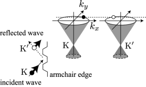
Figure 4: The armchair edge reflects the wave vector ${\bf k}=(k_{x},k_{y})$ of one valley into ${\bf k^{\prime}}=(-k_{x},k_{y})$ of another valley, and the two wave functions of the different valleys form a standing wave. The pseudospin is unchanged by the armchair edge. Note that the pseudospin for states near the K^′ point is not parallel to the vector ${\bf k^{\prime}}$, while the pseudospin for states near the K point is parallel to the vector ${\bf k}$.

To understand the behavior of the standing wave in more detail, the density of $\tau_{\alpha}$ was examined. The density for an eigenstate $\Psi(y)$ is defined by the expected value of $\tau_{\alpha}$ as $\tau_{\alpha}(x)\equiv\Psi^{\dagger}(x)\tau_{\alpha}\Psi(x)$. It is then straightforward to check from Eq. (94) that $\tau_{1}(x)\propto\pm\sin(2k_{x}x)$, $\tau_{2}(x)\propto\pm\cos(2k_{x}x)$, and $\tau_{3}(x)=0$. $\tau_{1}(x)$ vanishes near the armchair edge (at $x=0$), and $\tau_{2}(x)$ takes a maximum value at the edge. This behavior can be understood from Eq. (88), in which $\tau_{1}$ couples with $\phi_{\it r}(x)$. Since $\phi_{\it r}(x)$ is singular at $x=0$, $\tau_{1}(x)$ can not have a non-zero value at $x=0$. The result $\tau_{3}(x)=0$ indicates that time-reversal symmetry is preserved.

V.2 External Magnetic Field

Let us examine the Landau states near the armchair edge. The electromagnetic gauge field ${\bf A}=(0,-Bx)$ for an external magnetic field $B$ is included in the Hamiltonian $H({\bf r})$ of Eq. (5) by the substitution ${\bf{\hat{p}}}\to{\bf{\hat{p}}}-e{\bf A}$. The Hamiltonian satisfies $H({\bf-r})=\tau_{1}\sigma_{x}H({\bf r})\sigma_{x}\tau_{1}$, and therefore the solution can be written as

$$\Psi({\bf r})=\begin{pmatrix}\Psi_{\rm K}({\bf r})\cr\Psi_{\rm K^{\prime}}({\bf r})\end{pmatrix}=\begin{pmatrix}\Psi_{\rm K}({\bf r})\cr e^{ig}\sigma_{x}\Psi_{\rm K}({\bf-r})\end{pmatrix}.$$ (95)

Let $\Phi_{\rm K}({\bf r})$ be the solution for the case $\phi^{\rm q}(x)=0$. Then $\Phi_{\rm K}({\bf r})$ satisfies the following energy eigenequation:

$$v_{\rm F}\left[\sigma_{x}\hat{p}_{x}+\sigma_{y}(\hat{p}_{y}+eBx)\right]\Phi_{\rm K}({\bf r})=E\Phi_{\rm K}({\bf r}).$$ (96)

The solutions are the Landau states specified by integer $n$ and a center coordinate $X$ as [see Eq. (62)]

$$\Phi^{\rm LL}_{nX}({\bf r}) =C_{nX}e^{-i\frac{Xy}{{\it l}^{2}}}e^{-\frac{1}{2}\left(\frac{x-X}{\it l}\right)^{2}}$$

$$\times\begin{pmatrix}{\rm sgn}(n)\sqrt{2|n|}H_{|n|-1}\left((x-X)/{\it l}\right)\cr-iH_{|n|}\left((x-X)/{\it l}\right)\end{pmatrix}.$$ (97)

Applying the parity transformation ${\bf r}\to-{\bf r}$ to $\Phi^{\rm LL}_{{\rm K},nX}({\bf r})$, we obtain

$$\Phi^{\rm LL}_{{\rm K},nX}({\bf-r})=(-1)^{n+1}\sigma_{z}\Phi^{\rm LL}_{{\rm K},n-X}({\bf r}).$$ (98)

The matrix $\sigma_{z}$ on the right-hand side can be understood by applying the parity transformation ${\bf r}\to-{\bf r}$ to this energy eigenequation:

$$v_{\rm F}\left[\sigma_{x}\hat{p}_{x}+\sigma_{y}(\hat{p}_{y}+eBx)\right]\Phi_{\rm K}(-{\bf r})=-E\Phi_{\rm K}(-{\bf r}).$$ (99)

The negative sign in front of the right-hand side shows that the energy eigenvalue of $\Phi_{\rm K}(-{\bf r})$ is opposite to that of $\Phi_{\rm K}({\bf r})$. By substituting Eq. (98) into Eq. (95), we obtain

$$\Phi^{\rm LL}_{nX}({\bf r})=\begin{pmatrix}\Phi^{\rm LL}_{{\rm K},nX}({\bf r})\cr-ie^{ig}\sigma_{y}\Phi^{\rm LL}_{{\rm K},n-X}({\bf r})\end{pmatrix}.$$ (100)

By repeating the same argument given in the previous subsection, the following standing wave solutions are obtained:

$$\Psi^{\rm LL}_{nX\pm}(x)=N(x)\begin{pmatrix}\Phi^{\rm LL}_{{\rm K},nX}({\bf r})\cr\pm\sigma_{y}\Phi^{\rm LL}_{{\rm K},n-X}({\bf r})\end{pmatrix}.$$ (101)

There are no constraints for the value of $X$. It is then a straightforward calculation to check that $\tau_{1}(x)$ vanishes at the armchair edge.

VI Discussion and Summary

A realistic graphene edge may be a mixture of zigzag and armchair edges. Klusek et al. (2000); Giunta and Kelty (2001); Kobayashi et al. (2005); Niimi et al. (2005) The construction of the standing wave near the general edge is one of the interesting applications for our framework. We believe that the Hamiltonian in Eq. (5) can describe the low-energy electrons in a graphene plane with a general edge. However, note that this issue is related to the coherence length of the standing wave. In the present paper, we have not considered perturbations that break coherence, such as electron-phonon interaction. Interestingly, the electron-phonon interaction can also be represented as a deformation-induced gauge field. Sasaki and Saito (2008a); Sasaki et al. (2010c) Thus, the gauge field description for the graphene edge may be useful when we consider such issues.

The effective-mass model of Eq. (5) is equivalent to a chiral gauge theory for graphene that has been proposed by Jackiw and Pi. Jackiw and Pi (2007) Indeed, by applying $\sigma_{x}$ to $\Psi_{\rm K^{\prime}}({\bf r})$ in Eq.(4), the Hamiltonian in Eq. (5) may be rewritten as

$$H^{\prime}=v_{\rm F}\begin{pmatrix}\mbox{\boldmath$\sigma$}\cdot({\bf{\hat{p}}}+{\bf A}^{\rm q}({\bf r}))&\phi^{\rm q}({\bf r})\cr\phi^{\rm q}({\bf r})^{*}&-\mbox{\boldmath$\sigma$}\cdot({\bf{\hat{p}}}-{\bf A}^{\rm q}({\bf r}))\end{pmatrix},$$ (102)

which is the electronic Hamiltonian of the chiral gauge theory. They have investigated zero-mode solutions of the Hamiltonian with a topological vortex for ${\bf A}^{\rm q}({\bf r})$ on the background of Kekulé distortion for $\phi^{\rm q}({\bf r})$, in the context of fractionalization of quantum number. Hou et al. (2007); Chamon et al. (2008a, b) Our trial is then to study the graphene edge as a chiral gauge theory, although our results in this paper do not clarify fully the topological features of the graphene edge. It is interesting to note that one may find an advantage of a chiral gauge theory when we consider the real spins of the electrons. For example, the magnetism of the edge states may be understood as a parity anomaly phenomenon. Semenoff (1984); Sasaki and Saito (2008b) The various field-theoretical techniques may be utilized to explore the electronic properties near the edge. Note also that the perturbation which mixes the electrons in the two valleys has been examined in the studies on the topological defect in graphene. González et al. (1992); Lammert and Crespi (2000)

We have taken into account the edge as a part of the Hamiltonian. This strategy stems from the tight-binding lattice model, in which the edge is automatically included as a part of the Hamiltonian. A similar concept is found in the article by Berry et al. Berry et al. (1987), in which the authors modeled the edge using a mass term, $V({\bf r})\sigma_{z}$. They considered that a singularity of the mass $V({\bf r})\to\infty$ outside of the edge is necessary, in order to uniquely specify the pseudospin. We have observed a similar situation for the deformation-induced gauge field for the edge, that is, the field is singular at the edge. It is also interesting to note that $\phi^{\rm q}({\bf r})$ in Eq. (102) corresponds to the mass of a Dirac fermion, and that the armchair edge is a singular point as for the mass.

In summary, we have proposed a framework in which the edge is represented as the deformation-induced gauge field. We have used the framework to investigate the standing waves and edge states in the presence of a mass term and a magnetic field. The description of the edge using the deformation-induced gauge field is one attempt to better understand the edge. If we can describe the variety of edge structures as different configurations of a single gauge field, it provides a basis to further explore the properties near the edge.

Appendix A Rotation of Pseudospin

The configurations of the pseudospin field for three equivalent corners of the graphene BZ are not the same, as shown in Fig. 1. Consideration of this pseudospin behavior is given in this Appendix.

The tight-binding Hamiltonian can be written as Sasaki and Saito (2008a)

$$H({\bf k})=-\gamma_{0}\begin{pmatrix}0&\sum_{a}f_{a}({\bf k})\cr\sum_{a}f^{*}_{a}({\bf k})&0\end{pmatrix},$$ (103)

where $f_{a}({\bf k})\equiv e^{i{\bf k}\cdot{\bf R}_{a}}$ ($a=1,2,3$). Note that $f_{a}({\bf k})$ satisfies

$$f_{a}({\bf k}+n{\bf b}_{1}+m{\bf b}_{2})=f_{a}({\bf k})e^{-i\frac{2\pi}{3}\left(n+m\right)},$$ (104)

where $n$ and $m$ are integers. Hence, the representations of $H({\bf k})$, $H({\bf k}+{\bf b}_{1})$, and $H({\bf k}+{\bf b}_{1}+{\bf b}_{2})$ are different from each other, and are related via $H({\bf k}+{\bf b}_{1})=MH({\bf k})M^{-1}$ and $H({\bf k}+{\bf b}_{1}+{\bf b}_{2})=M^{-1}H({\bf k})M$, where

$$M=\begin{pmatrix}e^{+i2\pi/3}&0\cr 0&e^{-i2\pi/3}\end{pmatrix}=\exp\left(i\frac{2\pi}{3}\sigma_{z}\right).$$ (105)

For the solution $\Psi$ of $H({\bf k})$, we have the corresponding solution of the effective Hamiltonian at ${\bf k}+{\bf b}_{1}$ as $\Psi_{{\bf b}_{1}}=M\Psi$. $M$ is a rotational matrix for the pseudospin around the $z$-axis, so that the pseudospin of $\Psi$ and that of $M\Psi$ are related by rotation around the $z$-axis by an angle of $2\pi/3$. This explains why the configurations of the pseudospin field around the three equivalent K (K^′) points are different from each other, as shown in Fig. 1.

Next, we consider the effective Hamiltonians for three equivalent K (K^′) points. By expanding $f_{a}({\bf k})$ around the wave vector of the K point, ${\bf k}_{\rm F}=(4\pi/3a,0)$, we obtain $f_{a}({\bf k}_{\rm F}+{\bf k})=f_{a}({\bf k}_{\rm F})+if_{a}({\bf k}_{\rm F}){\bf k}\cdot{\bf R}_{a}+\cdots$. Using $f_{1}({\bf k}_{\rm F})=1$, $f_{2}({\bf k}_{\rm F})=e^{-i\frac{2\pi}{3}}$, and $f_{3}({\bf k}_{\rm F})=e^{+i\frac{2\pi}{3}}$, we have $H({\bf k}_{\rm F}+{\bf k})=v_{\rm F}\mbox{\boldmath$\sigma$}\cdot{\bf p}+\cdots$, where ${\bf p}=\hbar{\bf k}$ and $v_{\rm F}=3\gamma_{0}a_{\rm cc}/2\hbar$. Then $H({\bf k}_{\rm F}+{\bf b}_{1}+{\bf k})=Mv_{\rm F}\mbox{\boldmath$\sigma$}\cdot{\bf p}M^{-1}+\cdots$, and $H({\bf k}_{\rm F}+{\bf b}_{1}+{\bf b}_{2}+{\bf k})=M^{-1}v_{\rm F}\mbox{\boldmath$\sigma$}\cdot{\bf p}M+\cdots$ are obtained. The same argument can be applied to the K^′ points. For the K^′ point at $-{\bf k}_{\rm F}$, we obtain the effective Hamiltonian $H(-{\bf k}_{\rm F}+{\bf k})=v_{\rm F}\mbox{\boldmath$\sigma$}^{\prime}\cdot{\bf p}+\cdots$. It is then straightforward to obtain $H(-{\bf k}_{\rm F}+{\bf b}_{1}+{\bf k})=Mv_{\rm F}\mbox{\boldmath$\sigma$}^{\prime}\cdot{\bf p}M^{-1}+\cdots$, and $H(-{\bf k}_{\rm F}+{\bf b}_{1}+{\bf b}_{2}+{\bf k})=M^{-1}v_{\rm F}\mbox{\boldmath$\sigma$}^{\prime}\cdot{\bf p}M+\cdots$. This difference in the representations of the effective Hamiltonians does not cause a problem, because a coordinate transformation can be used to eliminate the $M$ matrix from one effective Hamiltonian (see also Appendices in Ref. Sasaki et al., 2008). Slonczewski and Weiss (1958) Here, we imply the coordinate transformation as the rotation of the $x$ and $y$-axes by $\pm 2\pi/3$. A coordinate transformation cannot alter the physics, and therefore the physical result derived from the effective Hamiltonians are the same. Rather, by using the change of the effective Hamiltonians under a translation given by the reciprocal lattice vectors, a constraint for the form of the effective Hamiltonians can be obtained. For example, the deformation Hamiltonian, $\mbox{\boldmath$\sigma$}\cdot{\bf A}^{\rm q}({\bf r})$, should transform in the same way as $\mbox{\boldmath$\sigma$}\cdot{\bf p}$. Therefore, we must have $H({\bf k}_{\rm F}+{\bf k})=v_{\rm F}\mbox{\boldmath$\sigma$}\cdot({\bf p}+{\bf A}^{\rm q})+\cdots$, $H({\bf k}_{\rm F}+{\bf b}_{1}+{\bf k})=Mv_{\rm F}\mbox{\boldmath$\sigma$}\cdot({\bf p}+{\bf A}^{\rm q})M^{-1}+\cdots$, and $H({\bf k}_{\rm F}+{\bf b}_{1}+{\bf b}_{2}+{\bf k})=M^{-1}v_{\rm F}\mbox{\boldmath$\sigma$}\cdot({\bf p}+{\bf A}^{\rm q})M+\cdots$. Otherwise, there would be three physically distinct effective Hamiltonians for the same K point. The deformation-induced gauge field ${\bf A}^{\rm q}({\bf r})$ satisfies this constraint, because

$$v_{\rm F}(A_{x}^{\rm q}({\bf r})-iA_{y}^{\rm q}({\bf r}))=\sum_{a}\delta\gamma_{0,a}({\bf r})f_{a}({\bf k}_{\rm F}).$$ (106)

Note that this equation is equivalent to Eq. (6). The phase factor of $e^{\mp i2\pi/3}$ appears when we change ${\bf k}_{\rm F}$ to ${\bf k}_{\rm F}+{\bf b}_{1}$ and to ${\bf k}_{\rm F}+{\bf b}_{1}+{\bf b}_{2}$, due to the factor of $f_{a}({\bf k}_{\rm F})$ on the right-hand side. A notable feature is that the constraint must be satisfied for a strong lattice deformation that corresponds to a large value of ${\bf A}^{\rm q}({\bf r})$. Therefore, the direction of the gauge field does not change, although the values of $\gamma_{0,a}({\bf r})$ are renormalized for a strong deformation.

Appendix B Edge states and Mass

The edge states in the presence of a mass term is of interesting, because the magnetism of the edge states is related to the generation of a local spin-dependent mass term due to the coulombic interaction. Sasaki and Saito (2008b) Here, we show how to obtain the edge states in the presence of a uniform mass term.

By substituting Eq. (43) into $H^{m}_{\rm K}(y)\Psi_{\rm K}(y)=E\Psi_{\rm K}(y)$, we obtain instead of Eq. (45)

$$\begin{split}&p_{x}+A^{\rm q}_{x}(y)+\hbar\frac{dg(y)}{dy}=D\cosh(2g(y)+f),\\ &\hbar\frac{d}{dy}\left(\frac{|y|}{\xi}\right)=D\sinh(2g(y)+f),\end{split}$$ (107)

where the variables $D$ and $f$ are respectively defined as

$$D\equiv\pm\frac{1}{v_{F}}\sqrt{E^{2}-m^{2}}\ {\rm and}\ \tanh(f)\equiv-\frac{m}{E}.$$ (108)

The solution of the second equation in (107) is

$$2g(y)+f=\begin{cases}\displaystyle-\sinh^{-1}\left(\frac{\hbar}{\xi D}\right)&(y<0),\\ \displaystyle+\sinh^{-1}\left(\frac{\hbar}{\xi D}\right)&(y>0).\end{cases}$$ (109)

The first equation in Eq. (107) is integrated with respect to $y$ from $-\xi_{g}$ to $\xi_{g}$. Considering the limit $\xi_{g}\to 0$, only singular functions of $A_{x}^{\rm q}(y)$ and $g(y)$ at $y=0$ can survive after the integration, so that we obtain

$$-\sinh^{-1}\left(\frac{\hbar}{\xi D}\right)=\int_{-\xi_{g}}^{\xi_{g}}A^{\rm q}_{x}(y)dy.$$ (110)

Using Eqs. (109) and (110), we see from the first equation in  (107) that

$$D=\frac{p_{x}}{\cosh\left(\int_{-\xi_{g}}^{\xi_{g}}A^{\rm q}_{x}(y)dy\right)}$$ (111)

holds except very close to the edge. From Eqs. (110) and (111), we see that $\xi$ is given by

$$\frac{1}{\xi}=-k_{x}\tanh\left(\int_{-\xi_{g}}^{\xi_{g}}A^{\rm q}_{x}(y)dy\right).$$ (112)

Note that $\xi$ in the presence of a mass term is identical to $\xi$ in the absence of the mass given in Eq. (51). The mass term would affect $\xi$, but this is not the case. From Eqs. (108) and (111) we obtain the energy eigenvalue

$$E=\pm\sqrt{m^{2}+(v_{F}D)^{2}}.$$ (113)

When $\int_{-\xi_{g}}^{\xi_{g}}A^{\rm q}_{x}(y)dy\to\infty$, we obtain $D=0$ and $E=\pm|m|$.

According to the definition of $f$ in Eq. (108), the sign of $f$ depends on the signs of both $m$ and $E$. Let us first consider the case of $E<0$, by which we have $f={\rm sign}(m)|f|$. Using this expression for $f$ in Eq. (109), we obtain

$$g(y)=\begin{cases}\displaystyle+\frac{1}{2}\int_{-\xi_{g}}^{\xi_{g}}A^{\rm q}_{x}(y)dy-\frac{1}{2}{\rm sign}(m)|f|&(y<0),\\ \displaystyle-\frac{1}{2}\int_{-\xi_{g}}^{\xi_{g}}A^{\rm q}_{x}(y)dy-\frac{1}{2}{\rm sign}(m)|f|&(y>0).\end{cases}$$ (114)

To determine $|f|$, we substitute Eq. (113) into Eq. (108), and considering that $\tanh(|f|)$ can be approximated as $1-2e^{-2|f|}$ for $|f|\gg 1$, we then have $|f|\approx\left|\int_{-\xi_{g}}^{\xi_{g}}A^{\rm q}_{x}(y)dy\right|$ for $\left|\int_{-\xi_{g}}^{\xi_{g}}A^{\rm q}_{x}(y)dy\right|\gg 0$. Since $\int_{-\xi_{g}}^{\xi_{g}}A^{\rm q}_{x}(y)dy\gg 0$ for the zigzag edge, Eq. (114) becomes

$$g(y)\approx\begin{cases}\displaystyle\int_{-\xi_{g}}^{\xi_{g}}A^{\rm q}_{x}(y)dy&(y<0),\\ \displaystyle 0\ &(y>0),\end{cases}$$ (115)

when $m<0$. The wave function of this eigenstate for $y>0$, which has unpolarized pseudospin, is negligible due to the normalization. Thus, the localized state with energy $E=-|m|$ in the valence energy band can appear near the edge only for $y<0$, and the wave function is given by $\Psi_{\rm K}(y<0)\propto\exp(-|y|/\xi){}^{t}(1,0)$. Similarly, for the case of $m>0$, we have

$$g(y)\approx\begin{cases}\displaystyle 0&(y<0),\\ \displaystyle-\int_{-\xi_{g}}^{\xi_{g}}A^{\rm q}_{x}(y^{\prime})dy^{\prime}&(y>0).\end{cases}$$ (116)

The corresponding wavefunction is has the pseudospin down state, which appears only for $y>0$ near the edge. It is noted that the mass term automatically selects the region where the edge state can appear, $y>0$ or $y<0$. This is reasonable, because we have used the particle-hole symmetry operator $\sigma_{z}$ to restrict the edge state only for $y>0$ or $y<0$ in Sec. IV.2. The particle-hole symmetry operator is nothing but the mass term.

References

- Kosynkin et al. (2009) D. V. Kosynkin, A. L. Higginbotham, A. Sinitskii, J. R. Lomeda, A. Dimiev, B. K. Price, and J. M. Tour, Nature 458, 872 (2009).
- Jiao et al. (2009) L. Jiao, L. Zhang, X. Wang, G. Diankov, and H. Dai, Nature 458, 877 (2009).
- Jia et al. (2009) X. Jia, M. Hofmann, V. Meunier, B. G. Sumpter, J. Campos-Delgado, J. M. Romo-Herrera, H. Son, Y.-P. Hsieh, A. Reina, J. Kong, et al., Science 323, 1701 (2009).
- Girit et al. (2009) C. O. Girit, J. C. Meyer, R. Erni, M. D. Rossell, C. Kisielowski, L. Yang, C.-H. Park, M. F. Crommie, M. L. Cohen, S. G. Louie, et al., Science 323, 1705 (2009).
- Liu et al. (2009) Z. Liu, K. Suenaga, P. J. F. Harris, and S. Iijima, Phys. Rev. Lett. 102, 015501 (2009).
- Stampfer et al. (2009) C. Stampfer, J. Güttinger, S. Hellmüller, F. Molitor, K. Ensslin, and T. Ihn, Phys. Rev. Lett. 102, 056403 (2009).
- Han et al. (2010) M. Y. Han, J. C. Brant, and P. Kim, Phys. Rev. Lett. 104, 056801 (2010).
- Gallagher et al. (2010) P. Gallagher, K. Todd, and D. Goldhaber-Gordon, Phys. Rev. B 81, 115409 (2010).
- Tanaka et al. (1987) K. Tanaka, S. Yamashita, H. Yamabe, and T. Yamabe, Synthetic Metals 17, 143 (1987).
- Kobayashi (1993) K. Kobayashi, Phys. Rev. B 48, 1757 (1993).
- Fujita et al. (1996) M. Fujita, K. Wakabayashi, K. Nakada, and K. Kusakabe, J. Phys. Soc. Jpn. 65, 1920 (1996).
- Nakada et al. (1996) K. Nakada, M. Fujita, G. Dresselhaus, and M. S. Dresselhaus, Phys. Rev. B 54, 17954 (1996).
- Klusek et al. (2000) Z. Klusek, Z. Waqar, E. A. Denisov, T. N. Kompaniets, I. V. Makarenko, A. N. Titkov, and A. S. Bhatti, Appl. Surf. Sci. 161, 508 (2000).
- Giunta and Kelty (2001) P. L. Giunta and S. P. Kelty, The Journal of Chemical Physics 114, 1807 (2001).
- Kobayashi et al. (2005) Y. Kobayashi, K. Fukui, T. Enoki, K. Kusakabe, and Y. Kaburagi, Phys. Rev. B 71, 193406 (2005).
- Niimi et al. (2005) Y. Niimi, T. Matsui, H. Kambara, K. Tagami, M. Tsukada, and H. Fukuyama, Appl. Surf. Sci. 241, 43 (2005).
- Wakabayashi et al. (2007) K. Wakabayashi, Y. Takane, and M. Sigrist, Phys. Rev. Lett. 99, 036601 (2007).
- Yamamoto et al. (2009) M. Yamamoto, Y. Takane, and K. Wakabayashi, Phys. Rev. B 79, 125421 (2009).
- Berry et al. (1987) M. V. Berry, F. R. S, and R. J. Mondragon, Proc. R. Soc. Lond. A 412, 53 (1987).
- McCann and Fal’ko (2004) E. McCann and V. I. Fal’ko, Journal of Physics: Condensed Matter 16, 2371 (2004).
- Akhmerov and Beenakker (2007) A. R. Akhmerov and C. W. J. Beenakker, Phys. Rev. Lett. 98, 157003 (2007).
- Akhmerov and Beenakker (2008) A. R. Akhmerov and C. W. J. Beenakker, Phys. Rev. B 77, 085423 (2008).
- Sasaki et al. (2010a) K. Sasaki, R. Saito, K. Wakabayashi, and T. Enoki, J. Phys. Soc. Jpn. 79, 044603 (2010a).
- Sasaki and Saito (2008a) K. Sasaki and R. Saito, Prog. Theor. Phys. Suppl. 176, 253 (2008a).
- Kane and Mele (1997) C. L. Kane and E. J. Mele, Phys. Rev. Lett. 78, 1932 (1997).
- Katsnelson and Geim (2008) M. Katsnelson and A. Geim, Phil. Trans. R. Soc. A 366, 195 (2008).
- Klein (1994) D. J. Klein, Chem. Phys. Lett. 217, 261 (1994).
- Klein and Bytautas (1999) D. Klein and L. Bytautas, Journal of Physical Chemistry A 103, 5196 (1999).
- Sasaki et al. (2006) K. Sasaki, S. Murakami, and R. Saito, J. Phys. Soc. Jpn. 75, 074713 (2006).
- Brey and Fertig (2006) L. Brey and H. A. Fertig, Phys. Rev. B 73, 235411 (2006).
- McClure (1956) J. W. McClure, Phys. Rev. 104, 666 (1956).
- Sasaki et al. (2009) K. Sasaki, Y. Shimomura, Y. Takane, and K. Wakabayashi, Phys. Rev. Lett. 102, 146806 (2009).
- Sasaki et al. (2010b) K. Sasaki, K. Wakabayashi, and T. Enoki, arXiv:1002.4443 (2010b).
- Sasaki et al. (2010c) K. Sasaki, H. Farhat, R. Saito, and M. S. Dresselhaus, Physica E 42, 2005 (2010c).
- Jackiw and Pi (2007) R. Jackiw and S.-Y. Pi, Phys. Rev. Lett. 98, 266402 (2007).
- Hou et al. (2007) C.-Y. Hou, C. Chamon, and C. Mudry, Phys. Rev. Lett. 98, 186809 (2007).
- Chamon et al. (2008a) C. Chamon, C.-Y. Hou, R. Jackiw, C. Mudry, S.-Y. Pi, and A. P. Schnyder, Phys. Rev. Lett. 100, 110405 (2008a).
- Chamon et al. (2008b) C. Chamon, C.-Y. Hou, R. Jackiw, C. Mudry, S.-Y. Pi, and G. Semenoff, Phys. Rev. B 77, 235431 (2008b).
- Semenoff (1984) G. W. Semenoff, Phys. Rev. Lett. 53, 2449 (1984).
- Sasaki and Saito (2008b) K. Sasaki and R. Saito, J. Phys. Soc. Jpn. 77, 054703 (2008b).
- González et al. (1992) J. González, F. Guinea, and M. A. H. Vozmediano, Phys. Rev. Lett. 69, 172 (1992).
- Lammert and Crespi (2000) P. E. Lammert and V. H. Crespi, Phys. Rev. Lett. 85, 5190 (2000).
- Sasaki et al. (2008) K. Sasaki, R. Saito, G. Dresselhaus, M. S. Dresselhaus, H. Farhat, and J. Kong, Phys. Rev. B 78, 235405 (2008).
- Slonczewski and Weiss (1958) J. C. Slonczewski and P. R. Weiss, Phys. Rev. 109, 272 (1958).