Electrometry using the quantum Hall effect in a bilayer 2D electron system

Abstract

We discuss the development of a sensitive electrometer that utilizes a two-dimensional electron gas (2DEG) in the quantum Hall regime. As a demonstration, we measure the evolution of the Landau levels in a second, nearby 2DEG as the applied perpendicular magnetic field is changed, and extract an effective mass for electrons in GaAs that agrees within experimental error with previous measurements.

The integer vonKlitzingPRL80 and fractional TsuiPRL82 quantum Hall effects are two of the most significant discoveries to emerge from several decades of intense study of two dimensional electron systems (2DESs). The density of states, which is central to understanding the physics of the quantum Hall effect, is not easily accessible via traditional transport measurements alone. Instead, the density of states is usually accessed via measurements of thermodynamic quantities such as the specific heat, GornikPRL85 magnetization, EisensteinPRL85 or compressibility. EisensteinPRB94 Studies of the magnetization of 2DESs in the quantum Hall regime have been particularly fruitful but at the same time extremely difficult. UsherJPCM09 Another way to extend beyond transport studies is to measure the chemical potential directly using single-electron transistor (SET) electrometers located on the heterostructure surface. HuelsPRB04 Although electrometry is considerably easier than magnetometry, SETs can be difficult to fabricate and are very sensitive to local fluctuations, causing significant measurement noise. A variant of this approach was pioneered by Kawano and Okamoto, who created a scanning electrometer using a quantum Hall effect device, KawanoAPL04 and used it to study Landau level scattering in a second 2DES. KawanoPRB04

In this work, we take these earlier electrometry measurements one step further to produce a sensitive electrometry system for studying a 2DES in the quantum Hall regime. Our electrometer uses the close proximity and strong capacitive coupling between two 2DESs in a double quantum well heterostructure – using one 2DES as a quantum Hall effect electrometer for the other. Our design is far simpler to implement than the previous designs by Huels et al. and Kawano and Okamoto. Additionally, the closer proximity and larger interface area should result in increased sensitivity and reduced noise compared to earlier implementations. KawanoAPL04 ; KawanoPRB04 As a demonstration of our device, we use it to map the evolution of the Landau levels (LLs) in a 2DES as a function of applied magnetic field. This technique could be used to investigate the effective mass $m^{*}$ and the Lande $g$-factor of 2D electron systems in less studied semiconductor heterostructures such as InGaAs/InP.

The device is fabricated on an AlGaAs/GaAs heterostructure (A2264) featuring two $20$ nm wide GaAs wells separated by a $30$ nm AlGaAs barrier. This gives an effective 2DES separation $d=50$ nm. Figures 1(a) and (b) show a top-view micrograph and a side-view schematic of the device, which is etched into a Hall bar configuration with NiGeAu ohmic contacts that penetrate both quantum wells. The device has five gates: a top-gate (shaded green) biased at $V_{\rm TG}$ that controls the electron density in the upper 2DES, and a set of four depletion gates (shaded white) to sever the connection between the upper 2DES and the ohmic contacts at the ends and sides of the Hall bar. All electrical measurements were performed at $\sim 50$ mK using four-terminal lock-in techniques with an excitation voltage of $100~{}\mu$V at $17$ Hz. Characterization of the device revealed that the upper (lower) 2DES has a mobility of $1.2\times 10^{6}$ cm${}^{2}/$Vs ($1.4\times 10^{6}$ cm${}^{2}/$Vs) and density $n_{\rm T}=2.00\times 10^{11}$ cm^-2 ($n_{\rm B}=1.98\times 10^{11}$ cm^-2) with the top-gate unbiased.

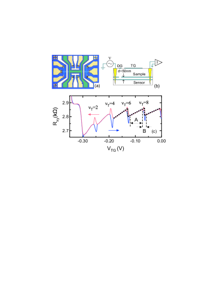
Figure 1:

(a) An optical micrograph of the device (b) A schematic of the device and measurement circuit. (c) The Hall resistance $R_{\rm xy}$ of the sensor 2DES (solid lines) vs top gate voltage $V_{\rm TG}$ at $B=0.924$ T for a sweep from $V_{\rm TG}=-0.35$ V to $0$ V (blue solid line) and back to $-0.35$ V (red solid line). The dotted black line is a guide to the eye for the ideal equilibrium behavior of $R_{\rm xy}$ to highlight the sharp jumps at even filling factors $\nu_{\rm T}$. The regions A and B correspond to those in Fig. 2(a)

We now discuss the operating concept for our device. The lower 2DES is used as a quantum Hall effect electrometer (hereafter referred to as the ‘sensor’) for the upper 2DES (hereafter ‘sample’). During the measurement, three of the four depletion gates are biased. This isolates the sample from the measurement circuit, aside from a connection to ground via the drain contact, which allows the density in the sample to respond to changes in $V_{\rm TG}$. Current thus passes only through the sensor 2DES, and we measure Hall resistance $R_{\rm xy}$ of that 2DES as our sensor output (the longitudinal resistance $R_{\rm xx}$ is measured simultaneously). It is important to note that $R_{\rm xy}$ is sensitive to both electric and magnetic fields, and can thus detect three distinct events: changes in the magnetic field $B$, changes in the sensor density due to changes in $V_{\rm TG}$ if the upper 2DES is depleted, and changes in the sensor density due to changes in the chemical potential $\Delta\mu_{\rm T}$ in the sample 2DES. The first allows us to set an operating point for the sensor, the second allows us to characterize the sensor, and the latter is the quantity we seek to measure. The coupling between the two 2DESs is capacitive, yielding a change in sensor density:

$$\Delta n_{\rm B}=\frac{\epsilon}{e^{2}d}\Delta\mu_{\rm T}$$ (1)

in response to a change in $\Delta\mu_{\rm T}$. The dielectric constant $\epsilon$ for the AlGaAs barrier between 2DESs can be directly measured, and is obtained from a comparison of the slopes of $n_{\rm T}$ vs $V_{\rm TG}$ when sample 2DES is populated, and $n_{\rm B}$ vs $V_{\rm TG}$ when then sample 2DES is depleted using a modified parallel-plate capacitor model. Low field measurements of $R_{\rm xy}$ are used to obtain $n_{\rm T}$ and $n_{\rm B}$, and we obtain $\epsilon=10.2\epsilon_{\rm 0}$. When mapping the Landau levels in the sample 2DES, the sensor 2DES will also be in the quantum Hall regime, resulting in maximum sensitivity in the middle of a quantum Hall transition where $R_{\rm xy}$ changes rapidly, and zero sensitivity in the quantum Hall plateau. Although this limits the operating range, an operating point that gives good sensitivity is easily established.

We now show a typical measurement obtained with our device. The chosen operating field $B=0.924$ T corresponds to a sensor 2DES filling factor $\nu_{\rm B}\approx 9.5$. In Fig. 1(c) we plot the sensor output $R_{\rm xy}$ against $V_{\rm TG}$ starting at $V_{\rm TG}=-0.35$ V and increasing to $0$ V (blue solid line), and then returning to $-0.35$ V (red solid line). For $V_{\rm TG}<V_{\rm depl}\sim-0.3$ V the sample 2DES is fully depleted and the top-gate acts directly on the sensor 2DES. In this region, decreases in $V_{\rm TG}$ reduce $n_{\rm B}$ and lead to a rising $R_{\rm xy}$. In contrast, when $V_{\rm TG}>V_{\rm depl}$ the sample 2DES is populated and changes in $R_{\rm xy}$ directly reflect changes in the sample 2DES chemical potential $\mu_{\rm T}$ via Eq. 1. There are two key features for the data in Fig. 1(c) for $V_{\rm TG}>V_{\rm depl}$. Firstly, the red and blue traces separate markedly when the sample 2DES filling factor $\nu_{\rm T}$ takes an even integer value. This hysteresis is due to non-equilibrium currents in the edge states of the sample 2DES, and will be discussed in detail elsewhere.

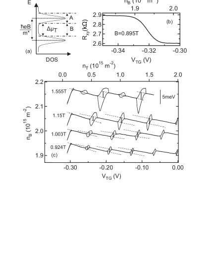
Figure 2:

(a) A schematic of the density of states (DOS) of the sample 2DES in the quantum Hall regime. (b) $R_{\rm xy}$ vs $V_{\rm TG}$ (bottom axis) and the corresponding $n_{\rm B}$ (top axis) at $B=0.895$ T showing the transition between $\nu=9$ (right) and $10$ (left). (c) The sensor 2DES density $n_{\rm B}$ vs $V_{\rm TG}$ (bottom axis) and the corresponding $n_{\rm T}$ (top axis) at four different operating points $B=0.924$, $1.003$, $1.15$ and $1.555$ T. The latter three traces have been vertically offset by $3$, $8$ and $16\times 10^{13}$ m^-2 for clarity. The equivalent scale in chemical potential is shown by the scale bar (upper right corner). The dashed black lines show the straight line fits to the non-hysteretic regions while the vertical solid lines at each hystersis ‘loop’ indicate the corresponding $\Delta\mu_{T}$ plotted in Fig. 3.

The second is the sawtooth structure in the measured $R_{\rm xy}$ when the sample 2DES is populated, as highlighted by the black dotted line at $V_{\rm TG}>-0.18$ V in Fig. 1(c). There are two mechanisms contributing to this structure – the periodic modulation of the density of states in the quantum Hall regime (see Fig. 2(a)) and the well-known negative compressibility effect observed in bilayer 2D systems. EisensteinPRL92 ; MillardAPL96 Starting in region A in Fig. 2(a), the chemical potential $\mu_{\rm T}$ coincides with a Landau level where the density of states (DOS) is large. Here small changes in $n_{\rm T}$ produce only small changes in $\mu_{\rm T}$, and this should produce a gentle increase in $R_{\rm xy}$ as $V_{\rm TG}$ is increased in the corresponding region in Fig. 1(c). Instead, we observe a gentle decrease in $R_{\rm xy}$ caused by negative compressibility, and this is consistent with earlier studies of bilayer 2D systems in the quantum Hall regime. EisensteinPRL92 Eventually we reach region B; here the DOS is very small, and small changes in $V_{\rm TG}$ produce a very rapid rise in $\mu_{\rm T}$. This rise overwhelms the negative compressibility to produce a corresponding sudden drop in $\Delta R_{\rm xy}$, as shown in Fig. 1(c).

Extracting $\Delta\mu_{\rm T}$ from the measured $\Delta R_{\rm xy}$ vs $V_{\rm TG}$ data involves two steps. First, we need to characterize the sensor 2DES to relate $\Delta R_{\rm xy}$ to $\Delta n_{\rm B}$, then we can simply use Eq. 1 to convert $\Delta n_{\rm B}$ to $\Delta\mu_{\rm T}$. The sensor characterization involves measuring $R_{\rm xy}$ versus $V_{\rm TG}$ with the sample 2DES depleted. This initially appears straightforward, but is more complicated because we set the operating point as the middle of a quantum Hall transition to maximize the sensitivity. To extract $\Delta\mu_{\rm T}$, we need to map $\Delta R_{\rm xy}$ to $\Delta n_{\rm B}$ for the whole transition, but as Fig. 1(c) highlights, only half of the transition is accessible if this is done at the operating point. We overcome this by performing the characterization at a slightly lower field $B=0.895$ T. As Fig. 2(b) shows, this allows us to map the entire transition without repopulating the sample 2DES. The $\sim 3\%$ difference between the operating point $B=0.924$ T and the characterization point $B=0.895$ T has a negligible effect on the resulting calibration. The $n_{\rm B}$ versus $V_{\rm TG}$ that results from applying the calibration in Fig. 2(b) to the data in Fig. 1(c) is shown as the bottom trace in Fig. 2(c). Finally, the relationship between $n_{\rm T}$ (top axis) and $V_{\rm TG}$ (bottom axis) in Fig. 2(b) is obtained from low field Hall measurements with $\Delta n_{\rm B}=\Delta V_{\rm TG}\times(4.01\times 10^{15}m^{-2}/V)$.

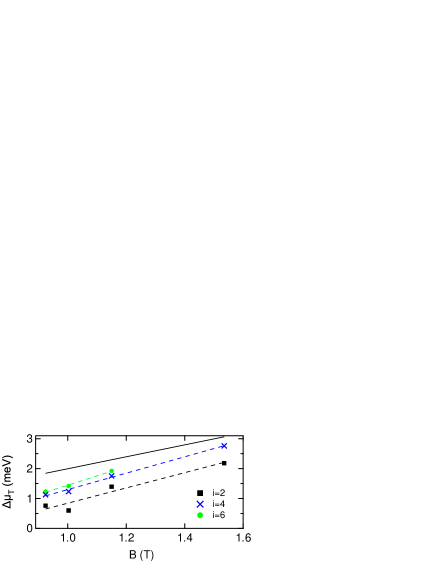
Figure 3:

The energy spacing $\Delta\mu_{\rm T}$ between adjacent Landau levels as a function of $B$. The transitions occur at the points where the filling factor $\nu_{\rm T}$ is an even integer $i$. The spacings have been measured for $i=2$, $4$ and $6$. The dashed lines are a straight line fit for each $i$, whereas the solid line shows the expected spacing $\hbar eB/m^{*}$.

We now focus on using our device to map the evolution of the three lowest spin-degenerate Landau levels $i=2$, $4$, and $6$ with $B$ for the sample 2DES, as shown in Fig. 3. In addition to the data for $B=0.924$ T discussed above, we obtain $n_{\rm B}$ vs $V_{\rm TG}$ data for three other operating points $B=1.003$, $1.15$, and $1.555$ T, each with its own sensor calibration performed at an appropriate nearby $B$. These three additional traces are presented in Fig. 2(c) and have been vertically offset for clarity. In obtaining the Landau level spacings $\Delta\mu_{\rm T}$ for Fig. 4, we need to overcome the obscuring effect of the hysteresis, and even in its absence, account for the contribution to $n_{\rm B}$ versus $V_{\rm TG}$ from the negative compressibility. We have devised a simple method for doing this which involves three steps. First we take linear fits to the sloped regions either side of the LL transition, shown by the dashed lines in Fig. 2(c). We then measure the vertical distance $\Delta n_{\rm B}$ between these two extrapolated fits at the LL transition point, as shown by the short vertical lines in Fig. 2(c). The transition point is assigned as the average of the position of the extrema in the up and down sweeps of the hysteresis loops. Finally, we obtain the corresponding chemical potential change $\Delta\mu_{\rm T}$ using Eq. 1. The use of the fits to the sloped regions adjacent to the transition in this process automatically corrects for the negative compressibility.

The extracted $\Delta\mu_{\rm T}$ values are plotted versus $B$ in Fig. 3. The solid line indicates the expected value of the LL spacing $\hbar eB/m^{*}$. We have used $m^{*}=0.058m_{\rm e}$ rather than the more typical value $m^{*}=0.067m_{\rm e}$ to account for the reduced effective mass at the low densities used in our experiment. ColeridgeSS96 The data for each LL follows a linear trend as indicated by the dashed lines in Fig. 3, however in each case, they sit well below the expected value (solid line). We attribute this discrepancy to Landau level broadening. EisensteinPRL85 This broadening is partly due to disorder, and increases as the mobility is lowered. A well known property of modulation doped 2DEGs is that the mobility decreases as the density is reduced. StormerAPL81 Thus at fixed $B$, the discrepancy between the data and the solid line should decrease for higher Landau levels $i$ where the density is higher, and we observe this to be the case in Fig. 3. The slopes of the linear fits to $\Delta\mu_{\rm T}$ versus $B$ for each $i$ are fairly consistent, and slightly higher than expected (i.e., the solid line). This is significant as the slope is directly related the effective mass $m^{*}$. Averaging the slopes obtained for different $i$ values gives $m^{*}=0.042m_{\rm e}$, which is qualitatively consistent with the findings of Coleridge et al., but $\sim 30\%$ lower than the value they obtain. ColeridgeSS96 Towards addressing this quantitative disagreement in $m^{*}$, we now briefly address the main sources of error in our experiment. Averaging across the three LLs, the error due to the linear fits is at most $11\%$, and is dwarfed by a more dominant contribution due the dependence of the disorder broadening on $n_{\rm T}$. StormerAPL81 Each data point for a given $i$ is obtained at a different $n_{\rm T}$, and we estimate this could increase in the measured slope by up to $25\%$, causing a decrease in the measured $m^{*}$ by a similar amount. Finally, we note that the density dependence of $m^{*}$ should lead to non-linearities in the measured $\Delta\mu_{\rm T}$ versus $B$ data, ColeridgeSS96 however these should be small over the range studied, and are not evident in the data presented in Fig. 3.

We conclude by discussing some potential improvements and applications for our technique. The key limiting factor in our device is the need to characterize and calibrate the sensor at each field where data is obtained. This is due to the lack of a back-gate, which prevents independent control of $n_{\rm B}$ in this device. With a back-gate, we could establish a feedback mechanism that uses the measured resistance to keep $n_{\rm B}$ constant. This would greatly simplify sensor calibration and ensuring maximum sensitivity over a greater $V_{\rm TG}$ range at arbitrary $B$. This would also allow the measurements in Fig. 3 to be obtained at fixed $n_{\rm T}$, overcoming the main source of error in measuring $m^{*}$ with this device.

In summary, we have developed a sensitive electrometry system that allows us to monitor the chemical potential of a 2D electron system in the quantum Hall regime as its density is changed at fixed magnetic field. Our electrometer operates by exploiting the strong capacitive coupling between two closely-spaced 2DESs in a double quantum well heterostructure. As a demonstration of this device, we have mapped the evolution of the Landau levels in a 2DES as a function of magnetic field, and used this to measure the electron effective mass, obtaining values that agree well with known literature values.

This work was funded by Australian Research Council (ARC). L.H.H. acknowledges financial support from the UNSW and the CSIRO.

References

- (1) :
- (2) K. von Klitzing, G. Dorda and M. Pepper, Phys. Rev. Lett. 45, 494 (1980).
- (3) D.C. Tsui, H. Störmer and A.C. Gossard, Phys. Rev. Lett. 48, 1559 (1982).
- (4) E. Gornik, R. Lassnig, G. Strasser, H.L. Störmer, A.C. Gossard and W. Wiegmann, Phys. Rev. Lett. 54, 1820 (1985).
- (5) J.P. Eisenstein, H.L. Störmer, V. Narayanamurti, A.Y. Cho, A.C. Gossard and C.W. Tu, Phys. Rev. Lett. 55, 875 (1985)
- (6) J.P. Eisenstein, L.N. Pfeiffer and K.W. West, Phys. Rev. B 50, 1760 (1994).
- (7) A. Usher and M. Elliott, J. Phys.: Condens. Matter 21, 103202 (2009).
- (8) J. Huels, J. Weis, J. Smet, K. von Klitzing and Z.R. Wasilewski, Phys. Rev. B 69, 085319 (2004).
- (9) Y. Kawano and T. Okamoto, Appl. Phys. Lett. 84, 1111 (2004).
- (10) Y. Kawano and T. Okamoto, Phys. Rev. B 70, 081308 (2004).
- (11) J.P. Eisenstein, L.N. Pfeiffer and K.W. West, Phys. Rev. Lett. 68, 674 (1992).
- (12) I. S. Millard, N. K. Patel, M. Y. Simmons, E. H. Linfield, D. A. Ritchie, and G. A. C. Jones, Appl. Phys. Lett. 68, 3323 (1996).
- (13) P.T Coleridge, M. Hayne, P. Zawadzki, and A.S. Sachrajda, Surf. Sci. 361, 560 (1996).
- (14) H. L. Störmer, A. C. Gossard, W. Wiegmann, and K. Baldwin, Appl. Phys. Lett. 39, 912 (1981).