New representations of $\pi$ and Dirac delta using the nonextensive-statistical-mechanics $q$-exponential function

Abstract

We present a generalization of the representation in plane waves of Dirac delta, $\delta(x)=\frac{1}{2\pi}\int_{-\infty}^{\infty}e^{-ikx}\,dk$, namely $\delta(x)=\frac{2-q}{2\pi}\int_{-\infty}^{\infty}e_{q}^{-ikx}\,dk$, using the nonextensive-statistical-mechanics $q$-exponential function, $e_{q}^{ix}\equiv[1+(1-q)ix]^{1/(1-q)}$ with $e_{1}^{ix}\equiv e^{ix}$, being $x$ any real number, for real values of $q$ within the interval $[1,2[$. Concomitantly, with the development of these new representations of Dirac delta, we also present two new families of representations of the transcendental number $\pi$. Incidentally, we remark that the $q$-plane wave form which emerges, namely, $e_{q}^{ikx}$, is normalizable for $1<q<3$, in contrast with the standard one, $e^{ikx}$, which is not.

I Introduction

Dirac delta is a distribution that is used in almost all branches of physics. Various representations of it have been discovered along the time. For example, it can be represented as a limit of a Gaussian or as a linear combination of plane waves, being the last one strongly related to the Fourier transform (FT), as we will show later.

Dirac delta, $\delta(x)$, obeys the following fundamental property:

$$\int_{-\infty}^{\infty}f(x)\delta(x)\,dx=f(0)\,,$$ (1)

where $f:\mathbb{R}\to\mathbb{C}$ is a well-behaved function. From the equation above, we can see that if $f(x)=1\;\forall x\in\mathbb{R}$, we get the normalization condition

$$\int_{-\infty}^{\infty}\delta(x)\,dx = 1\,.$$ (2)

Also, choosing $f(x)=f(0)e^{ikx}$ in (1), we obtain

$$\int_{-\infty}^{\infty}\delta(x)e^{ikx}\,dx=1\,,$$ (3)

i.e., the FT of $\delta(x)$ equals one. Therefore, using the expression of the inverse FT we obtain the following representation of Dirac delta:

$$\delta(x)=\frac{1}{2\pi}\int_{-\infty}^{\infty}e^{-ikx}\,dk\,,$$ (4)

which can be interpreted as a linear combination of plane waves. We can rewrite the expression above as

$$\delta(x)=\frac{1}{2\pi}\lim_{L\to\infty}\int_{-L}^{L}e^{-ikx}\,dk\,,$$ (5)

then, Dirac delta also can be represented as the following improper limit:

$$\delta(x)=\lim_{L\to\infty}\frac{\sin(Lx)}{\pi x}\,.$$ (6)

In 1988, a possible generalization of Boltzmann-Gibbs statistical mechanics was proposedTsallis1988 . This new theory, sometimes referred to as nonextensive statistical mechanics books , has been satisfactorily applied to handle a large number of physical phenomena (usually, metastable or quasi-stationary states of systems that are not consistent with the ergodic hypothesis; for example, systems in which long-range interactions or strong-correlations exist)UpadhyayaRieuGlazierSawada2001 ; DanielsBeckBodenschatz2004 ; ArevaloGarcimartinMaza2007a ; DouglasBergaminiRenzoni2006 ; LiuGoree2008 ; DeVoe2009 ; Borland2002a ; Queiros2005 ; BurlagaVinas2005 ; BurlagaNess2009 ; BakarTirnakli2009 ; CarusoPluchinoLatoraVinciguerraRapisarda2007 ; CarvalhoSilvaNascimentoMedeiros2008 ; PickupCywinskiPappasFaragoFouquet2009 ; CMS2010 . Furthermore, the elaboration of nonextensive statistical mechanics required the generalization of some mathematical functions (exponential, logarithm, etc.), operators (sum, product, Fourier transform, etc.) and theorems (central limit theorem)UmarovTsallisSteinberg2008 . Particularly, the generalization of the exponential function, namely, the $q$-exponential function is defined by

$$e_{q}^{x}\equiv[1+(1-q)x]_{+}^{\frac{1}{1-q}}\qquad\left(e_{1}^{x}\equiv e^{x}\right)\,,$$ (7)

for any $x\in\mathbb{R}$, where the symbol $[y]_{+}$ means that $[y]_{+}=y$, if $y\geq 0$, and $[y]_{+}=0$ if $y<0$. For pure imaginary $ix$, $e_{q}^{ix}$ can be defined to be the principal value of

$$e_{q}^{ix}\equiv[1+(1-q)ix]^{\frac{1}{1-q}}\qquad\left(e_{1}^{ix}\equiv e^{ix}\right)\,.$$ (8)

The main purpose of the present paper is to generalize the representation in plane waves of Dirac delta, introduced in equation (4), using the $q$-exponential function defined above.

II Representation of Dirac delta in $q$-plane waves

II.1 Proposition

Let us introduce the following quantity:

$$\delta_{q}(x)\equiv\frac{1}{c(q)}\int_{-\infty}^{\infty}e_{q}^{-i\xi x}\,d\xi\,\text{ with }q\in[1,2[\,,$$ (9)

which can be interpreted as a linear combination of $q$-plane waves, where $c(q)$ is a constant that may depend on $q$. We intend to show later that $\delta_{q}(x)=\delta(x)$ for all $1\leq q<2$.

Analogously to (5), we may write

$$\delta_{q}(x)=\frac{1}{c(q)}\lim_{\Lambda\to\infty}\int_{-\Lambda}^{\Lambda}e_{q}^{-i\xi x}\,d\xi\,\text{ with }q\in[1,2[\,,$$ (10)

therefore, by integrating, we can represent $\delta_{q}(x)$ as the following improper limit:

$$\delta_{q}(x)=\frac{2}{(2-q)c(q)}\lim_{\Lambda\to\infty}\frac{\sin\left\{\frac{2-q}{q-1}\arctan[(q-1)\Lambda x]\right\}}{x\left[1+(q-1)^{2}\Lambda^{2}x^{2}\right]^{\frac{2-q}{2(q-1)}}}\,\text{ with }q\in]1,2[\,.$$ (11)

II.2 The normalization constant $1/c(q)$ and the transcendental number $\pi$

The constant $c(q)$ must be equal to $2\pi$ at the limit $q\to 1^{+}$. Furthermore, $c(q)$ can be found from the normalization condition (2). Thus, we have

$$c(q)=\frac{2}{(2-q)}\lim_{\Lambda\to\infty}\int_{-\infty}^{\infty}\frac{\sin\left\{\frac{2-q}{q-1}\arctan[(q-1)\Lambda x]\right\}}{x\left[1+(q-1)^{2}\Lambda^{2}x^{2}\right]^{\frac{2-q}{2(q-1)}}}\,dx\,.$$ (12)

Using the change of variables $z=(q-1)\Lambda x$ we obtain

$$c(q)=\frac{2}{(2-q)}\lim_{\Lambda\to\infty}\int_{-\infty}^{\infty}\frac{\sin\left(\frac{2-q}{q-1}\arctan z\right)}{z(1+z^{2})^{\frac{2-q}{2(q-1)}}}\,dz\,.$$ (13)

As the integral does not depend on $\Lambda$, the limit symbol can be omitted. Therefore, we can write

$$c(q)=\frac{2}{(2-q)}\int_{-\infty}^{\infty}\frac{\sin[2\alpha(q)\arctan z]}{z\left(1+z^{2}\right)^{\alpha(q)}}\,dz\,,$$ (14)

where

$$\alpha(q)\equiv\frac{2-q}{2(q-1)}\,.$$ (15)

We easily verify that $\alpha:]1,2[\subset\mathbb{R}\to\mathbb{R^{+}}$ is a monotonically decreasing function of $q$.

In order to solve analytically the integral in (14), let us restrict to integer or half-integer values for $\alpha(q)$, more precisely, $1/2,1,3/2,\ldots$. This implies that $q$ will be allowed to assume just certain rational values within the interval $]1,2[$, namely $q=3/2,4/3,5/4,\ldots$. Using the change of variables $z=\tan\theta$ in Eq. (14), we obtain

$$c(q)=\frac{4}{2-q}\int_{0}^{\pi/2}\frac{\sin[2\alpha(q)\theta](\cos\theta)^{2\alpha(q)-1}}{\sin\theta}\,d\theta\,.$$ (16)

By using now the relation (53) proved in the Appendix, the expression above yields

$$c(q)=\frac{4}{2-q}\sum_{k=0}^{\left\lfloor\alpha(q)+\frac{1}{2}\right\rfloor-1}(-1)^{k}\binom{2\alpha(q)}{2k+1}\int_{0}^{\pi/2}d\theta\,(\cos\theta)^{4\alpha(q)-2k-2}(\sin\theta)^{2k}\,.$$ (17)

We remind that the Beta function, $B(x,y)$, is defined by

$$B(x,y)\equiv\int_{o}^{\pi/2}d\phi\,2(\cos\phi)^{2x-1}(\sin\phi)^{2y-1}\,\text{ with }x>0\text{ and }y>0\,,$$ (18)

which is related with Gamma function by

$$B(x,y)=\frac{\Gamma(x)\Gamma(y)}{\Gamma(x+y)}\,.$$ (19)

Therefore, using the expressions of Beta function shown above, Eq. (17) can be written as

$$c(q)=\frac{4\alpha(q)}{2-q}\sum_{k=0}^{\left\lfloor\alpha(q)+\frac{1}{2}\right\rfloor-1}(-1)^{k}\frac{\Gamma\left(2\alpha(q)-k-\frac{1}{2}\right)\Gamma\left(k+\frac{1}{2}\right)}{\Gamma(2k+2)\Gamma(2\alpha(q)-2k)}\,.$$ (20)

Let us rewrite now the expression above as

$$c(q)=\frac{2}{2-q}S_{n_{q}}\,,$$ (21)

where

$$S_{n_{q}}\equiv n_{q}\sum_{k=0}^{\left\lfloor\frac{n_{q}+1}{2}\right\rfloor-1}(-1)^{k}\frac{\Gamma\left(n_{q}-k-\frac{1}{2}\right)\Gamma\left(k+\frac{1}{2}\right)}{\Gamma(2k+2)\Gamma(n_{q}-2k)}\,\text{ with }n_{q}\equiv 2\alpha(q)\in\mathbb{N}\,.$$ (22)

When $n_{q}=1$ (which corresponds to $q=3/2$) we obtain straightforwardly that $S_{1}=\pi$. Also, it is straightforward to verify that $S_{2},S_{3},S_{4}$ are equal to $\pi$. Using a symbolic computation software, we also verified that from $n_{q}=1$ to $n_{q}=5000$ ($q=5002/5001$), $S_{n_{q}}=\pi$. Hence we state the following hypothesis:

$$\pi=n\sum_{k=0}^{\left\lfloor\frac{n+1}{2}\right\rfloor-1}(-1)^{k}\frac{\Gamma\left(n-k-\frac{1}{2}\right)\Gamma\left(k+\frac{1}{2}\right)}{\Gamma(2k+2)\Gamma(n-2k)}\,\quad\forall n\in\mathbb{N}\,.$$ (23)

We thus found a countable infinite family of representations of the transcendental number $\pi$ (see alsohypergeometricseriesbook ).

Using relation (23) in (21), the expression of $c(q)$ becomes

$$c(q)=\frac{2\pi}{2-q}\,.$$ (24)

In addition to the above, this relation has been checked numerically to be correct not only for certain rational values of $q$ within the interval $[1,2[$, but for all real numbers within that interval (see Fig. 1). Therefore, we conjecture that the integral which appears in (14) equals $\pi$ for any value of $q$ within that interval. Consistently, we obtain another infinite family of representations of the number $\pi$, namely

$$\pi=\int_{-\infty}^{\infty}\frac{\sin(2r\arctan z)}{z\left(1+z^{2}\right)^{r}}\,dz\,\quad\forall r\in\mathbb{R}^{+}\,.$$ (25)

This family is non countable and contains Eq. (23) as a particular case.

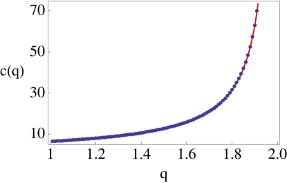
Figure 1: The blue dots were numerically obtained using expression (14), whereas the red continuous curve is the plot of $c(q)$ given by equation (24).

Finally, expressions (9) and (11) of $\delta_{q}(x)$ become respectively

$$\delta_{q}(x)=\frac{2-q}{2\pi}\int_{-\infty}^{\infty}e_{q}^{-i\xi x}\,d\xi\,\text{ with }q\in[1,2[$$ (26)

and

$$\delta_{q}(x)=\lim_{\Lambda\to\infty}\frac{\sin\left\{\frac{2-q}{q-1}\arctan[(q-1)\Lambda x]\right\}}{\pi x\left[1+(q-1)^{2}\Lambda^{2}x^{2}\right]^{\frac{2-q}{2(q-1)}}}\,\text{ with }q\in]1,2[\,.$$ (27)

II.3 Dirac delta behavior of the distribution $\delta_{q}(x)$

Let us define the following distribution

$$\Delta_{q}(x,\Lambda)\equiv\frac{\sin\left\{\frac{2-q}{q-1}\arctan[(q-1)\Lambda x]\right\}}{\pi x\left[1+(q-1)^{2}\Lambda^{2}x^{2}\right]^{\frac{2-q}{2(q-1)}}}\,\text{ with }q\in]1,2[\,,$$ (28)

which is related to $\delta_{q}(x)$ through

$$\delta_{q}(x)=\lim_{\Lambda\to\infty}\Delta_{q}(x,\Lambda)\,.$$ (29)

The plot of such a distribution (see Fig. 2) indicates that in the limit $\Lambda\to\infty$, $\Delta_{q}(x,\Lambda)$ will present a divergence at the origin and will be zero for all $x\not=0$, i.e., at first glance, $\delta_{q}(x)$ appears to be a representation of Dirac delta.

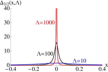
Figure 2: Plot of $\Delta_{3/2}(x,\Lambda)$ for different values of $\Lambda$. Similar results are obtained for any value of $q\in]1,2[$.

Let us now consider an analytic function, $f:\text{dom}\,f\subset\mathbb{R}\to\mathbb{C}$, which can be expanded in Taylor series around the origin such that the expression

$$f(x)=\sum_{k=0}^{\infty}\frac{f^{(k)}(0)}{k!}x^{k}$$ (30)

is valid for all $x\in\text{dom}\,f$. Then we have

$$\int_{-\infty}^{\infty}f(x)\delta_{q}(x)\,dx=\int_{\text{dom}\,f}f(x)\delta_{q}(x)\,dx\,.$$ (31)

Replacing $f(x)$ by its Taylor series, this expression yields

$$\int_{\text{dom}\,f}f(x)\delta_{q}(x)\,dx=\lim_{\Lambda\to\infty}\sum_{k=0}^{\infty}\frac{f^{(k)}(0)}{k!}\int_{\text{dom}\,f}\frac{x^{k-1}\sin\left\{\frac{2-q}{q-1}\arctan[(q-1)\Lambda x]\right\}}{\pi\left[1+(q-1)^{2}\Lambda^{2}x^{2}\right]^{\frac{2-q}{2(q-1)}}}\,dx\,,$$ (32)

in which we must remark that $q$ belongs to the interval $]1,2[$. If $\text{dom}\,f$ is a bounded interval of $\mathbb{R}$, i.e., $\text{dom}\,f=]a,b[$, with $a<b$, then using the change of variables $z=(q-1)\Lambda x$, we obtain

$$\int_{\text{dom}\,f}f(x)\delta_{q}(x)\,dx=\lim_{\Lambda\to\infty}\sum_{k=0}^{\infty}\frac{f^{(k)}(0)}{(q-1)^{k}\Lambda^{k}k!}\int_{(q-1)\Lambda a}^{(q-1)\Lambda b}\frac{z^{k-1}\sin\left(\frac{2-q}{q-1}\arctan z\right)}{\pi\left(1+z^{2}\right)^{\frac{2-q}{2(q-1)}}}\,dz\,.$$ (33)

The first term of the sum that appears above is

$$f(0)\lim_{\Lambda\to\infty}\int_{(q-1)\Lambda a}^{(q-1)\Lambda b}\frac{\sin\left(\frac{2-q}{q-1}\arctan z\right)}{\pi z\left(1+z^{2}\right)^{\frac{2-q}{2(q-1)}}}\,dz\,.$$ (34)

If $0<a<b$ or $a<b<0$, we straightforwardly see that expression above is equal to zero. If $a<0<b$, then using relation (25) we obtain that expression (34) is equal to $f(0)$. Finally, if we have either $a=0$ or $b=0$ (with $a<b$), then, also using relation (25) we obtain that expression (34) is equal to $f(0)/2$.

In order to analyze the next terms of the sum given in (33), let us first rewrite them as

$$\lim_{\Lambda\to\infty}f^{(k)}(0)J_{k}(\Lambda)\,\text{ with }k\in\mathbb{N}\text{ and }k>1\,,$$ (35)

where

$$J_{k}(q,\Lambda)\equiv\frac{1}{(q-1)^{k}\Lambda^{k}k!}\int_{(q-1)\Lambda a}^{(q-1)\Lambda b}\frac{z^{k-1}\sin\left(\frac{2-q}{q-1}\arctan z\right)}{\pi\left(1+z^{2}\right)^{\frac{2-q}{2(q-1)}}}\,dz\,\text{ with }k\in\mathbb{N}\text{ and }k>1\,.$$ (36)

$J_{k}(q,\Lambda)$ is a rapidly decreasing function of $k$ (see Fig. 3), which makes the sum given in (33) converge, consistently with the finiteness of the domain of $f$ in integral in Eq. (31). Moreover, from Fig. 3, we can infer that, in the limit $\Lambda\to\infty$, $J_{k}(q,\Lambda)\to 0$. Therefore, Eq. (33) implies

$$\int_{a}^{b}f(x)\delta_{q}(x)\,dx=\left\{\begin{array}[]{cc}f(0)&\text{if }a<0<b\\ f(0)/2&\text{if either }a=0<b\text{ or }a<0=b\\ 0&\text{if }0\not\in\,]a,b[.\end{array}\right.$$ (40)

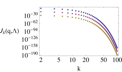
Figure 3: The $k$-dependence of $J_{k}(q,\Lambda)$, numerically obtained, considering $b=-a=1$, for $q=1.4$, and different values of $\Lambda$. From top to bottom, $\Lambda=10$, $\Lambda=10^{10}$, $\Lambda=10^{20}$.

In the case when $\text{dom}\,f$ is unbounded, i.e. if $\text{dom}\,f=]a,\infty[$, or $\text{dom}\,f=]-\infty,b[$, or $\text{dom}\,f=\mathbb{R}$, a similar analysis yields once again relation (40). Moreover, we numerically tested the validity of the mentioned relation using some types of functions and distributions (for example the Gaussian and the Lorentzian). Hence it seems reasonable to conjecture that, for a wide class of functions, $\delta_{q}(x)$ indeed is a representation of Dirac delta. Thus, we can finally write

$$\delta(x-x^{\prime})=\frac{2-q}{2\pi}\int_{-\infty}^{\infty}e_{q}^{-i\xi(x-x^{\prime})}\,d\xi\;\;\;(q\in[1,2[)\,.$$ (41)

III Square integrability of $q$-plane waves

Let us consider the following function:

$$\Psi(x)=Ne_{q}^{i\xi x}=N\left[\cos_{q}(\xi x)+i\sin_{q}(\xi x)\right]\,\text{ with }q\in]1,3[\text{ and }\xi\not=0\,,$$ (42)

which can be interpreted as a stationary $q$-plane wave, where the $q$-generalized trigonometric functions are defined, for any $x\in\mathbb{R}$, by (see also Borges1998 ):

$$\cos_{q}x\equiv\text{Re}\left(e_{q}^{ix}\right)=\frac{\cos\left\{\frac{1}{q-1}\arctan[(q-1)x]\right\}}{\left[1+(q-1)^{2}x^{2}\right]^{\frac{1}{2(q-1)}}}\,,$$ (43)

and

$$\sin_{q}x\equiv\text{Im}\left(e_{q}^{ix}\right)=\frac{\sin\left\{\frac{1}{q-1}\arctan[(q-1)x]\right\}}{\left[1+(q-1)^{2}x^{2}\right]^{\frac{1}{2(q-1)}}}\,.$$ (44)

We illustrate these functions in Fig. 4.

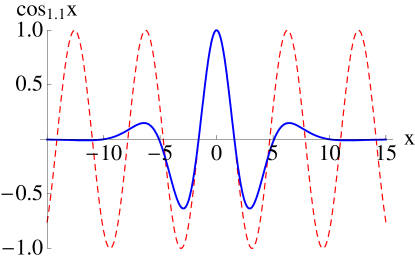
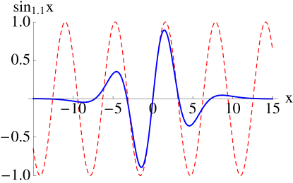
Figure 4: Top: $\cos_{1.1}x$ (continuous curve) and $\cos x$ (dashed curve). Bottom: $\sin_{1.1}x$ (continuous) and $\sin x$ (dashed). For $1\leq q<3$, $\cos_{q}x$ ($\sin_{q}x$) is an even (odd) function of $x$. For $1<q<3$, both functions $\cos_{q}x$ and $\sin_{q}x$ quickly decay when $|x|\to\infty$, in contrast with $\cos x$ and $\sin x$.

We will determine now the value of the constant $N$ using the normalization condition given by

$$\int_{-\infty}^{\infty}\Psi^{*}(x)\Psi(x)\,dx=1\,.$$ (45)

Thus, we have

$$\frac{1}{N^{2}}=\int_{-\infty}^{\infty}e_{q}^{-i\xi x}e_{q}^{i\xi x}\,dx\,,$$ (46)

which, using the definition of the $q$-exponential function given in (8), can be written as

$$\frac{1}{N^{2}}=\int_{-\infty}^{\infty}\frac{1}{\left[1+(q-1)^{2}\xi^{2}x^{2}\right]^{\frac{1}{q-1}}}\,dx\,.$$ (47)

Using the change of variables $\tan\theta=(q-1)|\xi|x$, this relation yields

$$\frac{1}{N^{2}}=\frac{1}{(q-1)|\xi|}\int_{-\pi/2}^{\pi/2}(\cos\theta)^{\frac{4-2q}{q-1}}\,dx\,.$$ (48)

Therefore, we obtain that the normalization constant is given by

$$N=\left[\frac{(q-1)|\xi|\Gamma\left(\frac{1}{q-1}\right)}{\sqrt{\pi}\Gamma\left(\frac{3-q}{2(q-1)}\right)}\right]^{\frac{1}{2}}\,.$$ (49)

Let us emphasize that the function $\psi(x)=e_{1}^{i\xi x}$ (plane wave) cannot be normalized, whereas $q$-plane waves, with $q\in]1,3[$, have a finite norm.

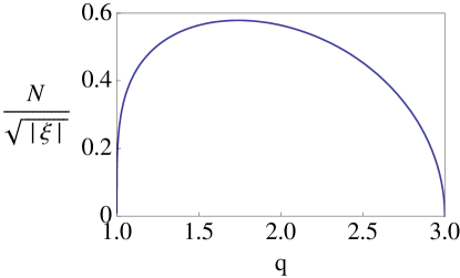
Figure 5: The normalization constant $N$ as a function of $q$. $N$ goes to zero in the $q\to 1$ limit, thus recovering the well known non-normalizability of the plane waves.

IV Conclusions

From the analytical and numerical results shown in section II, we conjecture Eq. (41), i.e., that $\delta_{q}(x)$ is indeed a generalization of the standard representation of Dirac delta in plane waves. Further research is welcome in order to establish which precise class of functions satisfy the relation (40).

Concomitantly, we found two new families of representations, namely expressions (23) and (25), of the transcendental number $\pi$. We tested the validity of such expressions for a set of values $n\in\mathbb{N}$ and $\alpha\in\mathbb{R}$. A demonstration is still required in order to formally establish these new families of representations of $\pi$.

A generalization of FT, namely, the so-called $q$-Fourier transform ($q$-FT) was developed in order to generalize the central limit theorem. The possible analytic expression of the inverse $q$-FT remains to be found. It is known that, using the representation in plane waves of Dirac delta together with the expression of the direct FT, it is possible to find the expression of the inverse FT. Consequently, we suppose that the present $q$-generalization of the representation in plane waves of Dirac delta might be helpful in searching for an analytic expression of the inverse $q$-FT. Moreover, the present new representations of Dirac delta could be useful to handle some integrals that may appear in the analysis of certain physical phenomena.

Finally, we prove a physically appealing property, namely that the $q$-plane wave form $e_{q}^{ikx}$ is square-integrable (in other words, normalizable) for $1<q<3$, in contrast with the standard form, $e^{ikx}$, which is not.

Appendix A Trigonometric identity

We establish here an expression for $\sin[2\alpha(q)\theta]$, with $2\alpha(q)\in\mathbb{N}$ and $\theta\in\mathbb{R}$, written in terms of $\sin\theta$ and $\cos\theta$. Firstly, we have

$$\sin[2\alpha(q)\theta]=\text{Im}\left[\left(\cos\theta+i\sin\theta\right)^{2\alpha(q)}\right],$$ (50)

then, using binomial expansion we have

$$\sin[2\alpha(q)\theta] = \text{Im}\left[\sum_{k=0}^{2\alpha(q)}\binom{2\alpha(q)}{k}(\cos\theta)^{2\alpha(q)-k}(\sin\theta)^{k}(i)^{k}\right]$$ (51)

$$= -\sum_{\stackrel{{\scriptstyle k=1}}{{\text{(odd)}}}}^{2\alpha(q)}(i)^{k+1}\binom{2\alpha(q)}{k}(\cos\theta)^{2\alpha(q)-k}(\sin\theta)^{k}.$$ (52)

Finally, this expression can be rewritten as follows:

$$\sin[2\alpha(q)\theta]=\sum_{k=0}^{\left\lfloor\alpha(q)+\frac{1}{2}\right\rfloor-1}(-1)^{k}\binom{2\alpha(q)}{2k+1}(\cos\theta)^{2\alpha(q)-2k-1}(\sin\theta)^{2k+1}$$ (53)

where we have used the floor function $\lfloor\,\,\rfloor$, defined, for any real number $x$, by $\lfloor x\rfloor=n$ such that $n\leq x<n+1$, with $n\in\mathbb{Z}$.

References

- (1) C. Tsallis, J. Stat. Phys. 52, 479 (1988).
- (2) M. Gell-Mann and C. Tsallis (eds), Nonextensive Entropy—Interdisciplinary Applications (Oxford University Press, New York, 2004); J. P. Boon and C. Tsallis (eds), Nonextensive Statistical Mechanics: New Trends, New Perspectives, Europhysics News 36, 185 (2005); C. Tsallis, Introduction to Nonextensive Statistical Mechanics (Springer, New York, 2009).
- (3) A. Upadhyaya, J.-P. Rieu, J.A. Glazier and Y. Sawada, Physica A 293, 549 (2001).
- (4) K.E. Daniels, C. Beck and E. Bodenschatz, Physica D 193, 208 (2004).
- (5) R. Arevalo, A. Garcimartin and D. Maza, Eur. Phys. J. E 23, 191 (2007).
- (6) P. Douglas, S. Bergamini and F. Renzoni, Phys. Rev. Lett. 96, 110601 (2006); G.B. Bagci and U. Tirnakli, Chaos 19, 033113 (2009).
- (7) B. Liu and J. Goree, Phys. Rev. Lett. 100, 055003 (2008).
- (8) R.G. DeVoe, Phys. Rev. Lett. 102, 063001 (2009).
- (9) L. Borland, Phys. Rev. Lett. 89, 098701 (2002).
- (10) S.M.D. Queiros, Quant. Finance 5, 475 (2005).
- (11) L.F. Burlaga and A.F.-Viñas, Physica A 356, 375 (2005).
- (12) L.F. Burlaga and N.F. Ness, Astrophys. J. 703, 311 (2009).
- (13) B. Bakar and U. Tirnakli, Phys. Rev. E 79, 040103(R) (2009).
- (14) F. Caruso, A. Pluchino, V. Latora, S. Vinciguerra and A. Rapisarda, Phys. Rev. E 75, 055101(R)(2007).
- (15) J.C. Carvalho, R. Silva, J.D. do Nascimento and J.R. de Medeiros, Europhys. Lett. 84, 59001 (2008).
- (16) R.M. Pickup, R. Cywinski, C. Pappas, B. Farago and P. Fouquet, Phys. Rev. Lett. 102, 097202 (2009).
- (17) CMS Collaboration, J. High Energy Phys. 02, 041 (2010).
- (18) S. Umarov, C. Tsallis and S. Steinberg, Milan J. Math. 76, 307 (2008); S. Umarov, C. Tsallis, M. Gell-Mann and S. Steinberg, J. Math. Phys. 51, 033502 (2010).
- (19) G. Gasper and M. Rahman, Basic Hypergeometric Series (Cambridge University Press, Cambridge, 2004); G.E. Andrews, The Theory of Partitions (Addison-Wesley, Reading, MA, 1976).
- (20) E.P. Borges, J. Phys. A 31, 5281 (1998).