Can One-Way Light Speed be Measured?
Comment on Greaves et al, Am. J. Phys. 77(10), 894-896 (2009)

Greaves et al[1] claim they devised an experiment to measure the one-way speed of light, something the vast majority of specialists consider wholly dependent on the particular synchronization convention chosen (with an infinitude of possibilities), and therefore not measurable in any absolute sense.[2] I argue here on the side of the majority.

1 THE AMBIGUITY IN ONE-WAY LIGHT SPEED

One-way light speed shares an interdependence with synchronization convention, i.e., the arbitrary setting of separate clocks at the photon emission and reception locations. The time difference between the first clock reading at the emission event and the second at the reception event is used with the known distance between clocks to calculate the speed. Different clock settings mean different one-way speeds. Round trip speed, on the other hand, whose emission and reception times are found using the same clock, does not require synchronization of distant clocks, is not subject to convention, and always (in vacuum) equals the universal constant $c$. If, for a given synchronization convention, the outgoing one-way speed is less than $c$, then the return one-way speed is greater than $c$, in such a way as to make the average round trip speed $c$. This conclusion is valid for any type of round trip path (back and forth in a straight line, loops, etc.)

One can either set distant clocks arbitrarily and use them to determine one-way light speed, or conversely, assume a particular one-way light speed and use it to set distant clocks.[3] In Einstein synchronization, the most common type, one assumes a one-way speed of $c$ and uses that to set distant clocks. In other synchronizations, one assumes a different one-way speed.[4]

Greaves et al’s purpose was to determine one-way light speed using the single clock at the detector, by varying the distance of one-way light travel and measuring the time variation on that single clock. Since only a single clock is used, the one-way speed would presumably be convention independent. Though this may seem reasonable at first, unfortunately it does not work, as explained below.

2 WHAT THE EXPERIMENT MEASURED

Fig. 1 is equivalent to, though slightly embellished from, the first figure in Greaves et al. The path from B to D is effectively horizontal, though, to make the figure legible, it is drawn as slightly inclined. We assume that the one-way speed of light from right to left in the horizontal direction equals $c^{-}<c$. This assumption means that if there were clocks at the sensor locations $L_{3}$ and $L_{2}$, they would be set relative to the detector clock at point $C$ such that they yield a one-way speed $c^{-}$.

The length of the cable of Fig. 1 is 23.73 m, and the time delay cited for an electromagnetic signal passing from one end of the cable to the other is 79 ns. In other communication, the lead author implied this was derived by taking half the time for a back and forth measurement, with reflection off the far end of the cable, using a single clock, though it may have simply been assumed. This yields a round trip signal speed in the cable of $c$ $\approx$ 3.00 $\times$ 10⁸ m/s, essentially the same as that in air.[5] It follows that the one-way speed of light in the cable would essentially equal the one-way speed in air.

If $c^{-}<c$, then as the cable from the sensor to the detector is looped to bring the sensor that was at L₃ to L₂, the time for the signal to pass the entire length of the cable does not, as claimed, stay the same. This is because, in the loop(s), the signal is traveling a round trip path, with average speed $c$, whereas elsewhere in the cable, it is traveling a one-way path with speed $c^{-}$.[6] For a straight cable aligned horizontally in Fig. 1 (lower configuration), the speed along the entire length would be $c^{-}$.

The contribution from the $L_{3}$ to $L_{2}$ section of the path to the measured time on the clock at detector C is the same, whether it is the visible light signal in air or the electromagnetic signal in the cable that is passing between $L_{3}$ and $L_{2}$. The closed loop length $L_{L}$ equals the distance between locations $L_{3}$ and $L_{2}$, which is the additional distance in the total path from the case with the sensor at L₃ (lower configuration) to that with the sensor at L₂ (upper configuration). Hence, the only measured time difference between the two sensor location cases is from the closed loop part of the cable.

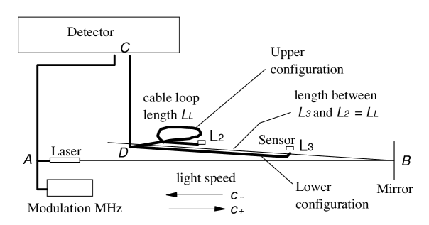
Figure 1: Sensor Location First at L₃, then at L₂.

And there, the electromagnetic signal speed equals $c$, meaning the experiment actually measures round trip speed in the loop, not one-way speed between $L_{3}$ and $L_{2}$.

Appendix I. Cable Signal Speed of 2/3 c

For a cable round trip signal speed of 2/3 c, start by taking $\Delta T_{base}$ as the time for the signal to pass along the cable from $L_{2}$ to point $D$, where the cable turns vertical in Fig. 1. The time for the signal to pass from $L_{3}$ to $D$ in the lower configuration of Fig. 1, where $c_{coax}^{-}$ is one way speed from right to left in the cable, is

$$T_{lower}=\Delta T_{base}+\frac{L_{L}}{c_{coax}^{-}}.$$ (1)

The time for the signal to pass from $L_{3}$ to $D$ in the upper configuration is

$$T_{upper}=\Delta T_{base}+\frac{L_{L}}{\textstyle{2\over 3}c}+\frac{L_{L}}{c^{-}}.$$ (2)

The difference is

$$T_{upper}-T_{lower}=\frac{L_{L}}{\textstyle{2\over 3}c}+\frac{L_{L}}{c^{-}}-\frac{L_{L}}{c_{coax}^{-}}.$$ (3)

If one uses Einstein synchronization, where $c^{-}=c$, and $c_{coax}^{-}=\textstyle{2\over 3}c$, then one has

$$T_{upper}-T_{lower}=\frac{L_{L}}{c},$$ (4)

where the time difference in (4) and $L_{L}$ were measured in the experiment.

Synchronizations other than Einstein’s change nothing that would be measured in (3), since the time difference in (3) is on a single clock, and this is unaffected by the synchronization choice for distant clocks. For any such other synchronization, $c^{-}$ would be known, and the constitutive value $c_{coax}^{-}$ would be determined by experiment. That experiment could be this one. Simply use the same experimental values and solve (3) for $c_{coax}^{-}$. In any synchronization choice, the time difference in (3) and (4), as well as $L_{L}$, are the same, so (4) holds for all synchronizations.

Appendix II. Römer Experiment

Some may consider the famous Römer experiment, which measured the speed of light via changes in light transmission time from Jupiter and its moons to be a one-way light speed determination. This effectively entails a time difference measured via a single clock on the Earth as this clock moves to different positions in the Earth’s orbit.

However, as shown in Ref. [2], the setting on a clock that is slowly transported relative to the speed of light (as the Earth clock is), will, upon arriving at a distant location, read the same time as a clock at that location that had been synchronized via the Einstein convention. That is, regardless of the synchronization convention used (and thus regardless of the one-way speed of light), the slowly transported clock will be set as though it had been Einstein synchronized.

Thus, any measurement with such a slowly transported clock will show $c$ for the one-way speed of light, as it is for Einstein synchronization. Hence, the Römer measurement does not measure one-way light speed in the usual sense.

There has, however, been more than a modicum of philosophical debate over whether slowly transported clocks should be taken as nature’s edict that an absolute synchronization (Einstein’s) exists. The present consensus is that it should not.

References

- [1] E. D. Greaves, A. M. Rodriguez, and J. Ruiz-Camacho, “A one-way speed of light experiment,” Am. J. Phys. 77(10) , 894-896 (2009).
- [2] There are a plethora of articles on this subject. A good summary of these, up to the date of publication, can be found in R. Anderson, I. Vetharaniam, G.E. Stedman, “Conventionality of Synchronization, Gauge Dependence, and Test Theories of Relativity,” Phys. Rep., 295, 3&4, 93-180 (1998).
- [3] Start with a clock at the emission point reading time T1. Assume a one-way outgoing speed of light in a certain direction of c’ (which can be other than c.) When the signal photon sent out along that direction reaches a second clock at distance D away, the time T2 on that clock needs to be such that c’= D/(T2 – T. So one resets that second clock so that the reading would have been what is required to measure a one-way speed c’. These two clocks have then been synchronized according to this particular convention.
- [4] The 3D treatment of one-way light speed is significantly more complicated, though consonant with the earlier statement that any possible round trip path for light in vacuum yields an average speed c.
- [5] This result seems strange, as signal speed in a coaxial cable is typically 2/3 that in air. See Appendix I for an analysis of that more realistic case.
- [6] Any folding back of the cable not in a loop would have the same net result. For example, an S curve would, from right-to-left, be a twice back and forth passage of the signal.