Abstract

The spectra of charged hadrons produced near mid-rapidity in d+Au, p+Au and n+Au collisions at $\sqrt{s_{\scriptscriptstyle{{\rm NN}}}}=200~{}\mbox{${\rm GeV}$}$ are presented as a function of transverse momentum and centrality. These measurements were performed using the PHOBOS detector at the Relativistic Heavy Ion Collider (RHIC). Nucleon-nucleus interactions were extracted from the d+Au data by identifying the deuteron spectators. The deuteron spectators were measured using two calorimeters; one that detected forward-going single neutrons and a newly installed calorimeter that detected forward-going single protons.

The large suppression of high-$p_{\mathrm{T}}$ hadron production in central Au+Au interactions relative to a naïve superposition of p+p̄ collisions has been interpreted as evidence of partonic energy loss in a dense medium. This interpretation is founded upon the absence of such suppression in the yield of d+Au collisions. The validity of using d+Au interactions in place of a nucleon-nucleus reference is tested. It is shown that hadron production in d+Au agrees with a simple binary collision scaling of hadron production in p+Au. An ideal reference for Au+Au collisions is constructed using a weighted combination of p+Au and n+Au yields and is found to be similar to the d+Au reference. Further, hadron production in p+Au interactions is compared to that of n+Au interactions. The single charge difference between a p+Au and a n+Au collision allows for a unique study of the ability of the interaction to transport the proton from the initial deuteron to mid-rapidity. However, no asymmetry between the positively and negatively charged hadron spectra of p+Au and n+Au interactions is observed at $\left<\smash[b]{\eta}\right>=0.8$.

Collision centrality was determined using several different observables, including those based on the multiplicity in different regions of pseudorapidity and those based on the amount of nuclear spectator material. It is shown that measurements made on small collision systems in the mid-rapidity region are biased by centrality variables based on the mid-rapidity multiplicity. Despite this bias, a smooth evolution with centrality is observed in the Cronin enhancement of hadrons produced in d+Au collisions. It is shown that this smooth progression is independent of the choice of centrality variable when centrality is parametrized by the multiplicity measured near mid-rapidity.

Thesis Supervisor: George S. F. Stephans
Title: Senior Research Scientist

This work is dedicated to the memory of
Ann-Marie, Donna and Theodore Elias.

Chapter 0 Strongly Interacting Matter

1 Forces of Nature

A successful description of the motion of matter is of fundamental importance to the understanding of nature. Classical descriptions of the mechanics of motion, developed during the Scientific Revolution around 1500-1700, postulated that objects tend to move in a straight line at a fixed speed. It followed that changes in the speed or direction of an object’s motion did not occur spontaneously, but were forced upon the object. The concept of forcing motion on an object through contact with the object is fairly intuitive. What is perhaps less obvious is how a force could act on an object at a distance and without contact. An example of such a force would be the ability of the Earth to accelerate flakes of snow to the ground (particularly in the Boston area).

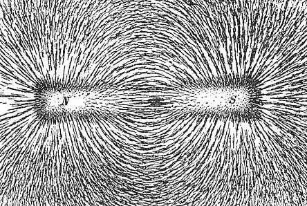
Figure 1: Iron filings reveal the field generated by a bar magnet [1].

Modern descriptions of the dynamics of objects have expanded upon these early concepts. Forces are no longer thought to act instantaneously at a distance. Instead, they are presumed to be mediated by fields, which describe physical quantities at every point in space. Force fields, for example, describe the magnitude and direction of the force that would be applied to an object at any particular point in space. Variations in a field progress at a finite speed. A visualization of a field is presented in Fig. 1 [1], which shows how iron filings orient themselves in a magnetic field. Indeed, studies of electricity and magnetism led to the foundation of theories of field dynamics. These studies not only showed that electricity and magnetism are two aspects of the same field, but that variations in this electromagnetic field travel through otherwise vacuous regions at the speed of light, $c\approx 3\times 10^{8}~{}\mbox{${\rm m/s}$}$. The latter observation led to the postulate that light itself is composed of waves propagating through the electromagnetic field.

These ideas were refined with the advent of quantum mechanics and special relativity. Relativity postulated that the laws of physics are the same in all inertial frames of reference; that is, to any observer not accelerating. It followed that, since the speed of light is an integral part of the descriptions of the electromagnetic field, light is always observed to be moving at a speed $c$ – regardless of how fast the light source or the observer may be moving. An important consequence of relativity was the equivalence of mass and energy. Expressed in what is likely the most famous equation of physics, $E=mc^{2}$, this concept reveals that an object at rest and under the influence of no forces still possesses a finite amount of energy proportional to its mass.

Quantum mechanics held that the motion of an object is not determined uniquely. Instead, a property of an object, such as its position, can be observed to take on a particular value only with some probability. That is, it is not possible to predict with certainty the outcome of a single measurement. However, predictions can be made regarding the possible outcomes of a measurement and the likelihood with which each outcome could occur. It was possible to interpret quantum mechanics as describing the dynamics of a wavefunction, rather than the dynamics of an object. The value of this wavefunction at any point in space is related to the probability of observing the object at that point.

The current understanding of the dynamics of objects combines all of the concepts discussed above into a relativistic quantum field theory. This description of nature is built upon the existence of fields which describe the possible states of a physical system (the universe) and the probability with which the system might be found in each state. When such an observation is performed, the field will be measured not as a continuous wave, but rather as indivisible, dimensionless packets called ‘quanta’ or ‘particles.’ Because the fields are consistent with relativity, energy in a field can be converted to mass, and vice-versa. Thus, the number of particles observed in the field can change; increasing as energy is converted to mass, and decreasing as mass is converted to energy. The dynamics of the particles are driven by interactions between various fields.

Generation	Particle	Symbol	Charge	Mass (MeV$\kern-1.49994pt/\kern-1.19995ptc^{2}$) [2]
First	Electron Neutrino	$\nu_{e}$	$0$	$<2\times 10^{-6}$
	Electron	$e^{-}$	$-1$	$0.511$
[1pt/4pt] Second	Muon Neutrino	$\nu_{\mu}$	$0$	$<0.19$
	Muon	$\mu^{-}$	$-1$	$105.7$
[1pt/4pt] Third	Tau Neutrino	$\nu_{\tau}$	$0$	$<18.2$
	Tau	$\tau^{-}$	$-1$	$1777$

Table 1: The leptons. For each particle, there is an oppositely charged antiparticle (not shown). The neutrino masses listed here are effective masses, see [2].

Generation	Particle	Symbol	Charge
First	Up	$u$	$+2/3$
	Down	$d$	$-1/3$
[1pt/4pt] Second	Charm	$c$	$+2/3$
	Strange	$s$	$-1/3$
[1pt/4pt] Third	Top	$t$	$+2/3$
	Bottom	$b$	$-1/3$

Table 2: The quarks. Each quark listed here can carry one of the three types of color charge: red, blue or green (see Sect. 2). For each of these 18 quarks, there is an antiparticle with an opposite electric and color charge.

In the Standard Model, nature is characterized by a set of fields that describe the fundamental building blocks of matter and by another set of fields that mediate their interactions: the forces. The building blocks of matter are divided into two distinct groups known as quarks and leptons. For example, an everyday object such as a book is composed of an unimaginably large number of atoms. Each atom consists of a tiny nucleus surrounded by a cloud of electrons (the electron is the most famous lepton). The nucleus is made up of a collection of tightly bound protons and neutrons, each of which is itself composed of quarks. All of the fundamental particles, quarks and leptons, are quanta of their respective fields. For each particle, there exists an antiparticle. An antiparticle is also a quantum of its field, so it shares certain properties with its corresponding particle, such as mass. However, other properties of an antiparticle known as additive quantum numbers, such as electric charge, are exactly opposite to those of its corresponding particle [3]. Currently, it is believed that there are three generations of both leptons and quarks. The particles in a given generation share certain properties that influence how they react with the quanta of other fields [4]. The current understand of the properties of elementary particles can be found in [2]. A list of the lepton generations is presented in Table 1 and a list of the quark generations is shown in Table 2. Because free quarks are not observed, as will be discussed in Sect. 2, determining the mass of the quarks is the subject of study; see [2] for current estimates.

The interactions between particles of matter are thought to be governed by four forces. Gravity is likely the most familiar force, yet a description of gravity in terms of relativistic quantum field theories has proven extraordinarily difficult [5], to the extent that gravity is not included in the Standard Model. However, gravity is so incredibly weak compared to the other fundamental forces – in the physical phenomena discussed in this thesis – that it can be safely ignored.

The second least powerful force is known as the weak force. Unlike gravity, the weak force has a very small range, about $10^{-18}~{}\mbox{${\rm m}$}$, and is not observed to bind objects together. Instead, the weak force mediates interactions between the quanta of matter fields, both quarks and leptons, in such a way as to allow a change in the type, or flavor, of the initial particle(s). For example, the decay of a neutron to a proton, known as beta decay, is governed by the weak force. In this interaction, a down quark changes flavor to an up quark through the process $d\rightarrow ue^{-}\bar{\nu}_{e}$.

The electromagnetic force mediates the interaction between electrically charged particles. The charge of any particle can be expressed in discrete units of the magnitude of an electron’s charge, as is done in Tables 1 and 2. The electromagnetic force is the most prevalent force in everyday experience, and consequently is the most well understood force [6]. All molecular binding and chemical reactions are the result of electromagnetic interactions. In addition, contact forces in the macroscopic world can be attributed to the repulsion of atoms near the surface of opposing objects.

Such repulsive electromagnetic forces also cause protons in an atomic nucleus to repel each other. Yet despite this fierce repulsion, the protons are bound together, along with neutrons, into a very small volume – the radius of a nucleus is over ten thousand times smaller than the radius of an atom. Thus the protons and neutrons attract each other through some force that is far stronger than the electromagnetic repulsion of the protons. This force is aptly, if not creatively, named the strong force. The strong force is thought to be so powerful that the binding of protons and neutrons in a nucleus is merely a residual effect of the interactions between quarks in the nucleons (a nucleon being either a proton or a neutron). This residual force is analogous to the residual electromagnetic force that binds atoms into molecules; see [7] for a discussion of atomic molecules and [8] for a discussion of the residual nuclear force. The strong force is not experienced by leptons, nor by the quanta of the other force fields. It is described in the Standard Model by the relativistic quantum field theory known as Quantum Chromodynamics (QCD).

2 Quantum Chromodynamics

Quantum Chromodynamics (QCD) is a relativistic quantum field theory that is believed to describe the strong force. The theory describes the dynamics of six quark fields, the quanta of which are listed in Table 2. Each quark carries an electric charge as well as a different kind of charge known as color. There are three types of color charge: red, blue and green. A quark carries one of the three colors, red, blue or green, while an antiquark carries one of the three anticolors. For example, the antiparticle of an up quark carrying a red color charge, $u_{r}$, would be an antiup quark carrying an “antired” charge, $\bar{u}_{\bar{r}}$. This is analogous to electromagnetism, in which there is a single type of electric charge that can take on two values, positive or negative. The interactions of particles carrying color charge are mediated by eight force fields, the quanta of which are massless particles known as gluons. The rationale for eight gluon fields is rooted in the fact that gluons themselves carry color: each gluon carries both a color charge and an anticolor charge. The various color states of the gluons can be written as

$$r\bar{b},r\bar{g},b\bar{g},b\bar{r},g\bar{b},\frac{r\bar{r}-b\bar{b}}{\sqrt{2}},\frac{r\bar{r}+b\bar{b}-2g\bar{g}}{\sqrt{6}}$$ (1)

where the latter two gluons can be understood through a quantum mechanical description. For example, the $(r\bar{r}-b\bar{b})/\sqrt{2}$ gluon can be thought of as being at once both a red, antired gluon and a blue, antiblue gluon that has a 50/50 chance of being observed as a $G_{r\bar{r}}$ or as a $G_{b\bar{b}}$. The ninth possible combination of colors,

$$\frac{r\bar{r}+b\bar{b}+g\bar{g}}{\sqrt{3}}$$ (2)

is not a part of QCD, nor of nature. Such a gluon would be what is known as a color singlet, that is, it would carry no net color. This would allow other colorless particles (such as protons) to exchange the gluon, and would facilitate strong interactions over macroscopic distances, assuming this gluon is also massless. Clearly, there is no evidence that such a gluon exists.

gluonexchange (1,7)(1,7) (110,62) thin i1,o1 i2,o2 $u_{g}$i1 $\bar{u}_{\bar{g}}$i2 $u_{b}$o1 $\bar{u}_{\bar{b}}$o2 fermioni1,v1,o1 fermiono2,v2,i2 gluon,label=$G_{g\bar{b}}$,label.dist=0.09wv1,v2

Figure 2: An example of a quark-antiquark interaction through the exchange of a gluon. The flow of time in the diagram is up-wards; the horizontal direction represents spatial separation. Note that the quarks change color after interacting.

Particle [Quark Content]	Symbol	Mass (MeV$\kern-1.49994pt/\kern-1.19995ptc^{2}$)	Mean Lifetime (s)
Proton $[uud]$	p	$938.3$	stable
Neutron $[udd]$	n	$939.6$	$898$
[1pt/4pt] Positive Pion $[u\bar{d}]$	$\pi^{+}$	$139.6$	$2.603\times 10^{-8}$
Negative Pion $[d\bar{u}]$	$\pi^{-}$	$139.6$	$2.603\times 10^{-8}$
Neutral Pion $[(d\bar{d}+u\bar{u})/\sqrt{2}]$	$\pi^{0}$	$135.0$	$0.83\times 10^{-16}$
Positive Kaon $[u\bar{s}]$	$K^{+}$	$493.7$	$1.237\times 10^{-8}$
Negative Kaon $[s\bar{u}]$	$K^{-}$	$493.7$	$1.237\times 10^{-8}$

Table 3: Properties of some common hadrons [9]. The mean lifetimes shown are for free particles. The stability of the proton is the subject of active experimental and theoretical study [10, 11].

An example of an interaction between an up quark and an antiup quark in one dimension is shown in Fig. 2. A study of such simple gluon exchanges shows that the lowest energy, and therefore most stable, bound states of quarks – called hadrons – are (a) a combination of three quarks each having a different color, called a baryon, and (b) a combination of a quark and its antiquark, called a meson; see [9] for a discussion. This is in good agreement with observation. The proton and neutron are the most common baryons observed in nature. Two mesons that are abundantly produced in high energy hadron collisions are the pion and the kaon. The quark content of these particles is listed in Table 3.

ggqq (1,7)(1,14) (100,62) thin i1,o1 i2,o2 $G_{r\bar{g}}$i1 $G_{g\bar{r}}$i2 $\bar{u}_{\bar{g}}$o1 $u_{g}$o2 fermiono1,v1 fermionv2,o2 fermion,label=$u_{r}$v1,v2 gluoni1,v1 gluoni2,v2

(a) Quark Exchange

ggggexg (1,7)(1,14) (100,62) thin i1,o1 i2,o2 $G_{r\bar{g}}$i1 $G_{g\bar{r}}$i2 $G_{b\bar{g}}$o1 $G_{g\bar{b}}$o2 gluonv1,o1 gluonv2,o2 gluon,label=$G_{r\bar{b}}$,label.dist=0.09wv1,v2 gluoni1,v1 gluoni2,v2

(b) Gluon Exchange

gggg (1,7)(1,14) (75,62) thin i1,o1 i2,o2 $G_{r\bar{g}}$i1 $G_{g\bar{r}}$i2 $G_{b\bar{g}}$o1 $G_{g\bar{b}}$o2 gluonv1,o1 gluonv1,o2 gluoni1,v1 gluoni2,v1

(c) Direct Interaction

Figure 3: Examples of gluon-gluon interactions. 3(a) Interaction via quark exchange. 3(b) Interaction via gluon exchange. 3(c) Direct interaction.

One of the most striking differences between QCD and electromagnetism is the fact that the quanta of the QCD fields carry color charge. Consequently, gluons can directly interact with other gluons, as shown in Fig. 3(b) and 3(c). There is no analog for this in electromagnetism; the quantum of that force, the photon, does not carry electric charge and therefore does not interact directly with other photons. This direct interaction between the gluon fields has severe effects on the dynamics of colored particles. An example of this is the coupling strength between colored particles, parametrized by $\alpha_{s}=g_{s}^{2}/4\pi$, where $g_{s}$ is related to the amount of color charge carried by the particles. Fluctuations of the quark and gluon fields in the vicinity of a colored particle are capable of altering the effective coupling strength, $\alpha_{s}^{\rm eff}$.

There is an electromagnetic analogy to this, in which fluctuations of the electron field result in the production of “virtual” electron-positron pairs. These fluctuations are just that: pairs of particles which are produced and annihilated, in otherwise empty space, in such a short amount of time that their presence is not directly observable, hence the label ‘virtual.’ In the presence of a (non-virtual) electron, these virtual pairs can be pictured as forming a cloud around the electron. Pairs in this cloud become polarized by the electron and result in an effective reduction, or screening, of the electric charge felt by a test particle at some distance from the electron [12]. As the test particle approaches the electron and pierces the cloud of virtual particles, the strength of this screening is reduced.

In QCD, on the other hand, there is evidence that just the opposite happens. While fluctuations in the quark fields surrounding a colored particle may screen its color charge, in a perfect analogy to electromagnetism, fluctuations in the gluon fields can enhance the particle’s color charge. This enhancement is due entirely to the self-interaction of the gluon fields. The effective coupling strength of the strong force felt by a test particle at short distances has been calculated [13], and is presented in Eq. 3. In experimental observation, however, it is not possible to measure the distance between a test particle and the colored object – nor is it very meaningful. Thus instead of distance, the effective charge seen by a test particle is parametrized by the amount of momentum transfered between the test particle and the colored object. Large momentum transfers correspond to small distances.

$$\alpha_{s}^{\rm eff}\left(Q^{2}\right)\approx\frac{4\pi}{\left(11-\frac{2}{3}n_{f}\right)\ln\left(Q^{2}/\Lambda^{2}\right)}$$ (3)

in natural units ($c=\hbar=1$), where $Q$ is the momentum transfer, $n_{f}$ is the number of quark flavors (six) and $\Lambda$ is a constant of nature, roughly 200 MeV$\kern-1.49994pt/\kern-1.19995ptc$. That is, for $Q\gg\Lambda$, Eq. 3 gives a reasonable approximation of the effective coupling strength. It is clear from this equation that as the momentum transfer increases, and shorter distances are probed, the effective coupling strength approaches zero. This property of the strong force is known as asymptotic freedom [14, 15, 16, 17]. On the other hand, for small momentum transfers, the effective coupling strength increases without bound. Of course, Eq. 3 is not thought to be a good approximation of the QCD coupling strength, or of nature, for very small values of momentum transfer. Nevertheless, the implication is that while the strong force is weak at very small distances, it is strong at large distances.

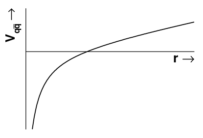
Figure 4: The qualitative form of the potential between a (very heavy) quark and its antiquark, as estimated in [18]. For large separation, the potential becomes linear, and for closer separation, it falls as $-1/r$.

This might seem to suggest that the strong force should be observable, and indeed quite powerful, on macroscopic scales. After all, distances on the order of centimeters are certainly large distances compared to the relevant length scale $\Lambda^{-1}$ – by about thirteen orders of magnitude. This hypothesis can be explored by studying the static, one dimensional potential between a quark and its antiquark (with anticolor). This potential has been estimated for very heavy quarks, and is thought to be valid for quark-antiquark separations larger than $\sim 0.1~{}\mbox{${\rm fm}$}$ [18, 19]. For relatively small $q-\bar{q}$ separations, the potential has a $-1/r$ dependence, analogous to the static electric potential between two charged particles. However, at larger separations, the potential becomes linear, as shown in Fig. 4. Thus, at large distances, the force between a quark and an antiquark is the same regardless of how far apart the quarks are separated. This implies that the quarks are always bound, as it would take an infinite amount of energy to separate the quarks completely. Notice further that the $q-\bar{q}$ system in question is colorless; thus this potential is relevant to the study of mesons. For a discussion of the static potential between three quarks, thus relevant for baryons, see [20]. This property of QCD, in which particles that interact via the strong force (i.e. “strongly interacting” particles) form colorless bound states from which they cannot escape, is known as confinement.

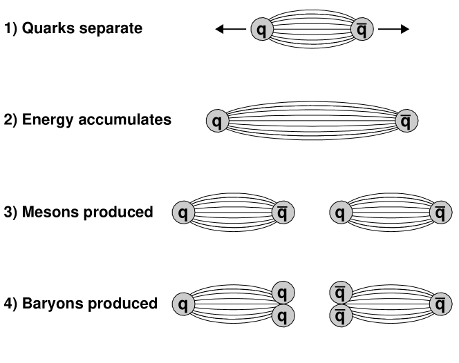
Figure 5: A cartoon of hadron production in the color flux tube, or string breaking, model [21]. As the quarks separate, energy accumulates in the field. When the energy is more than double the quark mass, it becomes possible for a $q-\bar{q}$ pair to be produced. The produced quarks will bind to the original quarks to form two colorless mesons. Baryon production can happen in an analogous fashion, through the production of a diquark, antidiquark pair [22].

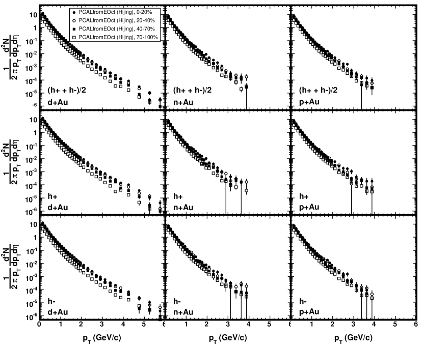
Figure 5: The invariant yield of $(\mathrm{h}^{+}+\mathrm{h}^{-})/2$, $\mathrm{h}^{+}$ and $\mathrm{h}^{-}$ in four centrality bins determined using HIJING and the EPCAL centrality variable. The trigger efficiency as a function of EPCAL was determined using EOct. The spectra for d+Au, n+Au and p+Au are shown in separate columns. Only statistical errors are shown.

A further implication of the linear form of the potential between two quarks is revealed by the consideration of the quarks being drawn apart by some external agent. Because the force between the quarks is constant, the external agent will need to continuously add energy into the system to separate the quarks. Eventually, the amount of energy added will be greater than the rest mass of a quark-antiquark pair. It would then be possible for this energy to be converted into mass. The probability of this happening increases with the amount of energy added to the system [21]. Thus, as shown in Fig. 5, new quarks would be produced, and all quarks in the system would remain confined to colorless bound states. This is an example of hadronization, the process by which the fundamental particles of QCD are formed into the hadrons that are observed in nature.

The confinement of colored objects into colorless hadron states sheds light on the question of strong forces at macroscopic distances. It can be shown that the fields generated by a single, free color source would have an infinite amount of energy [23]; thus free colored states do not exist on their own. Further, as suggested by the example described above, colored particles cannot be freed from their colorless bound states; attempts to do so simply result in the production of more colorless hadrons. Thus, all colored particles remain confined to colorless bound states, and of course, (color) neutral particles do not interact when they are separated by distances much larger than their size. Interactions occur only when these objects are close enough that their internal composition becomes discernible. For example, colorless protons and neutrons in the nucleus of one atom of a molecule, where the separation between nucleons in the nucleus is $\sim 1.5~{}\mbox{${\rm fm}$}$ [24], are bound together by the residual strong force. However, these nucleons do not experience any appreciable strong force interactions with nucleons in neighboring atoms, as the separation between atoms is roughly one hundred thousand times larger than the size of a nucleon.

Thus, in cold nuclear matter, quarks and gluons are confined to colorless protons and neutrons. It should be noted, however, that the structure of hadrons is far more interesting than the quark content shown in Table 3 might suggest, and is the subject of ongoing study [25] (see [26, 27] for more information). These composite particles in turn settle into bound states to form nuclei. This matter is “cold” by definition, since it is in its ground state, the state in which the system stores the least amount of kinetic and potential energy. The behavior of strongly interacting matter under very different conditions – high temperature and high density – can be studied experimentally by colliding highly energetic nuclei.

3 Heavy Ion Collisions

The theory of QCD is thought to provide a valid description of strongly interacting matter. Unfortunately, calculating the dynamics of realistic systems using the full theory of QCD has proven exceedingly difficult. Consequently, experimental studies of strongly interacting matter are valuable not only in their ability to test the predictions of QCD, but in their ability to explore more exotic and less well understood systems. One of the most effective experimental techniques that enables such studies is the analysis of collisions of highly energetic nuclei, i.e. heavy ions. As two relativistic nuclei (relativistic in that their kinetic energy is much greater than their rest mass) collide, a system of strongly interacting matter may be produced. The dynamics of this system is a subject of intense study. It is expected that the produced system will consist of densely packed quarks, antiquarks and gluons.

1 The Density of Produced Matter

The energy density of the system produced in Au+Au collisions, in which each nucleus carries 19.7 ${\rm TeV}$ of kinetic energy, can be estimated using the so-called Bjorken estimate [28]. The energy density will, of course, be the amount of energy contained in some volume. The volume of the system produced in a head-on, or “central,” collision can be approximated as a cylinder, with a transverse area equal to that of the nuclei, $\mathscr{A}$, and some reasonable length. The length of the cylinder will clearly increase with time as the produced system expands, and it is reasonable to believe that the length of the cylinder will expand much more rapidly than the radius, due to the large initial longitudinal momenta of the nuclei. Thus, the estimation of the length of the cylinder is rather an estimate of the time at which it is appropriate to consider the energy density of the system. Since it is clear that typical length scales of the strong force must be on the order of the size of the proton, it is natural to estimate the energy density at $\tau_{0}\sim 1\to 2~{}\mbox{${{\rm fm}/c}$}$. Finally, it is necessary to estimate the amount of energy contained in the produced system. This energy should be directly related to the energy of hadrons emitted by the system. Since it is the energy in the produced system that is of interest, and not the energy carried by the initial nuclei, hadrons produced with a momentum that is roughly transverse to the initial nuclei should provide the best estimate of the energy of this matter. Thus, the energy density can be estimated as follows.

$$\epsilon_{0}\approx\frac{\left<E_{T}\right>d\!N/\mathit{dy}}{\tau_{0}\mathscr{A}}\approx\frac{\sqrt{(0.500~{}\mbox{${\rm GeV}$})^{2}+m_{\pi}^{2}}\;(700)\;(3/2)}{(1\to 2~{}\mbox{${\rm fm}$})\;\pi\;(6.5~{}\mbox{${\rm fm}$})^{2}}\approx 4\to 2~{}\mbox{${\rm GeV}$}/\mbox{${\rm fm}$}^{3}$$ (4)

where $\left<E_{T}\right>$ is the average transverse energy of emitted hadrons and $d\!N/\mathit{dy}$ is the number of hadrons in the mid-rapidity region. It was assumed that the vast majority of produced particles are pions [29] having an average transverse momentum of 500 MeV$\kern-1.49994pt/\kern-1.19995ptc$ [30]. It was further assumed that all three pion species – positive, negative and neutral – are produced in equal number, so that the total number of particles is $(3/2)\times d\!N_{\mathrm{ch}}/\mathit{dy}$, where $d\!N_{\mathrm{ch}}/\mathit{dy}$ is the multiplicity (number of produced particles) of charged hadrons. Using the mid-rapidity multiplicity measured in [31], the total number of particles is $(3/2)\times 700$. The radius of the nucleus was taken to be about 6.5 ${\rm fm}$; see Fig. 10 on page 10. While this estimate of the energy density of the matter produced in a high energy Au+Au collision is fairly rough, it does imply that the matter is an order of magnitude greater than that of a gold nucleus, $\sim 160~{}\mbox{${\rm MeV}$}/\mbox{${\rm fm}$}^{3}$, and at least five times as dense as that of a proton. Approximating the volume of a proton by a sphere with a radius of 0.8 ${\rm fm}$, $\epsilon_{\rm p}~{}\approx~{}0.938~{}\mbox{${\rm GeV}$}/\left[(4/3)\pi(0.8~{}\mbox{${\rm fm}$})^{3}\right]\approx~{}0.450~{}\mbox{${\rm GeV}$}/\mbox{${\rm fm}$}^{3}$. This high density suggests that the relevant constituents of the matter produced in these collisions are likely to be the quarks, antiquarks and gluons themselves, rather than the hadrons which are subsequently observed. It is an exciting prospect that this loss of “hadronic degrees of freedom” may mean that the strongly interacting matter produced in these collisions is not confined (at least for some amount of time) to hadrons, but only to the larger volume of the system as a whole. However, no direct evidence has been presented, and the topic of deconfinement remains a subject of extensive inquiry [32, 33].

The energy density is an informative property, as it expresses the density of the system in a way that is independent of the specific make-up of the matter. However, it is also important to estimate the relative abundance of baryons and antibaryons in the produced medium. This is typically done experimentally by measuring the ratio of antiprotons to protons produced in the mid-rapidity region. Antiprotons generated by the collision will be produced together with protons, via pair production [34]. Because the initial nuclei consist solely of baryons, and because the number of baryons minus antibaryons is unchanged in any interaction, the antiproton to proton ratio is an indication of how many of those initial protons get “transported” to mid-rapidity during the collision, relative to the number that are produced.

$$\frac{\bar{\rm p}}{\rm p}=\frac{\bar{\rm p}_{\rm produced}}{{\rm p}_{\rm produced}+{\rm p}_{\rm transported}}$$ (5)

Thus, not only is the ratio a measure of how baryon rich the produced medium is, but also of how effective the collision is at changing the momenta of the initial nucleons. It is instructive to examine the extreme values this ratio may assume. A $\bar{\rm p}/{\rm p}$ ratio of one implies that the produced medium is completely baryon free and none of the original nucleons are transported to the mid-rapidity region. The term ‘baryon free,’ refers to the net number of baryons in the system: the number of baryons in excess of the number of antibaryons. Such a baryon free system could be created by very distinct scenarios. In the first, the initial nuclei pass through each other completely, none of the nucleons are stopped, and the medium produced in the central region is the result of an excited vacuum caused by the collision [35]. In the second scenario, the nuclei stop completely upon colliding, creating an extremely dense medium that comes to equilibrium and then explodes, sending the nuclei receding in directions opposite to their initial momenta. The third scenario is a combination of the other two, in which the quarks of the initial nuclei pass through each other completely, while the gluons stop completely and form a very dense medium that then explodes, as described in [36]. The $\bar{\rm p}/{\rm p}$ ratio is not able to distinguish between these very different models of particle production. At the opposite extreme, a $\bar{\rm p}/{\rm p}$ ratio near zero implies that the produced medium is intensely baryon rich. That is, essentially no pair production of baryons occurs, so any protons observed near mid-rapidity must have been transported from the initial nuclei.

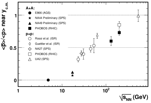
Figure 6: The $\bar{\rm p}/{\rm p}$ ratio measured near mid-rapidity in nucleus-nucleus and nucleon-nucleon collisions, as a function of energy per nucleon pair in the center of mass frame. The plot is from [30, 37]. The data are from [38, 39, 40, 41, 42, 43, 44, 45, 46, 47].

The ratio of antiprotons to protons observed in the mid-rapidity region of both nucleus-nucleus and nucleon-nucleon collisions is presented as a function of the collision energy per nucleon pair in Fig. 6 [30, 37]. This shows that the $\bar{\rm p}/{\rm p}$ ratio rises with collision energy in both systems. Thus, the higher the kinetic energy of the initial hadrons, the more important pair production processes become compared to baryon transport. Additionally, these results show that the net baryon content of the matter produced in the central region of such collisions decreases with increasing collision energy.

2 The Temperature of Produced Matter

It is clear that heavy ion collisions are capable of producing matter that is both far more dense and far less baryon rich than ordinary nuclear matter. This begs the question of whether this dense matter, which is presumably expanding rapidly, has sufficient time to achieve equilibrium, and if so, does it have a high temperature. This is an important question, since studies of QCD have suggested that a system of strongly interacting matter that is in equilibrium and is sufficiently hot may form a phase of matter known as a Quark-Gluon Plasma (QGP) [48, 49]. Conceptually, this phase of matter would consist of a soup of quarks, antiquarks and gluons that are not confined to hadrons. Due to the extremely large temperature, these elementary particles would have large kinetic energies on average. Thus, interactions between them would occur with large momentum transfers – or equivalently, at short distances – and according to Eq. 3, such interactions would be governed by weak coupling. Thus the constituents a QGP should be relatively mobile. The presence of mobile color charges, quarks, would be expected to screen any long distance interactions; hence the term ‘plasma.’ It is this state of matter that is thought to have been predominant in the very early universe, during the first 10 $\mu{\rm s}$ after the big bang, prior to the formation of hadrons [50]. Whether such a weakly interacting QGP is produced in heavy ion collisions is the subject of ongoing investigation, and will be discussed in Ch. 7 and 8 of this thesis.

Regardless of the phase of matter produced in heavy ion collisions, it is valuable to estimate how hot the matter is so that its dynamics can be described in terms of its temperature. However, direct measurements of the temperature of the produced matter are not possible. In macroscopic systems, such a measurement is typically performed by allowing the system in question to come to thermal equilibrium with a second system whose behavior as a function of temperature is well understood, i.e. a thermometer, and observing the temperature of the second system. Clearly, such a technique cannot be applied to the matter produced by a heavy ion collision. However, inspiration can be drawn from astronomy, where the spectrum of light radiated by a star is used to determine its surface temperature [51].

In an analogous fashion, the spectrum of particles emitted by the matter produced in a heavy ion collision can be used to estimate its temperature. Unfortunately, the particles measured by a heavy ion experiment will not be the same particles that were radiated by the initially produced medium. This fact can be understood by following the evolution of the heavy ion collision. The beginning of the collision can be taken to be the point at which the distance between the nuclei is much smaller than their longitudinal size, but before any particle production has occurred. The energy density is at its maximum at this point, but is not particularly interesting, since it does not describe any produced matter. During some time following this, substantial particle production will occur. Given what is known about the typical strength of QCD interactions, the time for this particle production is expected to be roughly $\,{\buildrel<\over{{}_{\sim}}}\,1~{}{\mbox{${{\rm fm}/c}$}}$. How particles are actually produced is in principle described by QCD, however the difficulty of carrying out calculations in the full theory has lead to the creation of a host of more simplified models. After this early period, the produced quarks, antiquarks and gluons may come to thermal equilibrium. It is at this point that the energy density estimate of Eq. 4 is applicable, and at which a QGP may be formed. As this dense system of strongly interacting matter expands, it will cool and the elementary particles will form hadrons. Again, QCD should in principle describe the process of hadronization, but as it involves long-range interactions, calculations using the full theory have not yet been developed and simplified hadronization models are preferred. At some point during the expansion of this hadron gas, inelastic collisions between hadrons will cease, and the relative yield of particle species, such as the $\bar{\rm p}/{\rm p}$ ratio, will be completely determined. This stage of the collision is therefore known as chemical freeze-out. Finally, as this gas of hadrons expands further, even elastic collisions will cease. At this point, the momentum spectrum of each particle species is determined, since the particles will not interact further before being detected by an experimental apparatus. Therefore, this stage of the collision is known as thermal freeze-out.

From this picture, it is clear that a temperature which is naïvely extracted from the spectrum of hadrons observed in an experiment will not describe the temperature of the very dense medium formed early in the collision. Instead, this temperature would describe the system as it was at thermal freeze-out. Therefore, to estimate the temperature of interest, it would be necessary either (a) measure the spectra of particles that reach thermal freeze-out at much earlier times in the collision, such as photons, or (b) to model the full collision process such that the final measured spectra could be described in terms of the properties of the initial dense medium. The spectra of penetrating probes such as photons are the subject of study, see [52], for example. However, there is presently no model of heavy ion collisions which is able to predict all aspects of the collision in a coherent manner. Instead, simpler models that describe certain aspects of the collision can be used to extract the temperature of the produced particle system during a certain stage of the collision.

These models are typically based on hydrodynamics or statistical mechanics. One such hydrodynamical model is known as a blast-wave [53], since it assumes thermal emission of particles from a rapidly expanding shell. This model can be used to extract the temperature of the system at the point of thermal freeze-out. Typical freeze-out temperatures given by this model for central Au+Au collisions at a center of mass energy of 39.4 ${\rm TeV}$, or 200 ${\rm GeV}$ per nucleon pair, are ${\rm T_{\rm f.o.}}\sim 110~{}{\mbox{${\rm MeV}$}}$ [54, 55]. It should be noted that the temperature parameter of this model is highly anti-correlated with the velocity at which the shell is expanding.

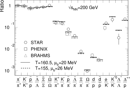
Figure 7: Relative hadron yields measured in Au+Au collisions at a center of mass energy of 200 ${\rm GeV}$ per nucleon pair. The statistical model was used to fit these ratios to extract the temperature at chemical freeze-out. The three right-most ratios, involving resonances, were not included in the fits. The dashed line shows the fit to the data excluding the $\bar{\rm p}/{\pi^{-}}$ and $\bar{\phi}/{K^{-}}$ ratios [56].

Statistical models are better suited to describe the collision at the chemical freeze-out stage [57]. One such model uses the grand canonical ensemble to estimate the yield of various particle species. In this statistical ensemble, one envisions having a large set of systems, each of which is identically prepared and is in equilibrium with some external bath of energy and particles. These systems would then be allowed to evolve, and the properties of the average system are determined. Thus, in the grand canonical ensemble, the number of particles of each type is allowed to vary. Physical rules that constrain the number of particles, for example the conservation of the number of net baryons in the system, are obeyed only on average. These models display impressive success at fitting the relative yields of a wide variety of particle species with a single set of parameters. The temperature of the matter produced in Au+Au collisions at a center of mass energy of 200 ${\rm GeV}$ per nucleon pair at chemical freeze-out, as estimated by one such model, is shown in Fig. 7 [56].

While the success of these models seems to suggest that the matter produced in high energy heavy ion collisions was able to reach equilibrium, it should be noted that statistical models are also able to describe hadron production in more elementary collisions, where no thermalized medium is expected [58, 59]. Nevertheless, the results of these models seem to present a consistent picture. At the latest stage of the collision, thermal freeze-out, the system seems to have a temperature of $\sim 110~{}\mbox{${\rm MeV}$}$. Before the system had ceased inelastic interactions, at chemical freeze-out, its temperature was higher, $\sim 160~{}\mbox{${\rm MeV}$}$. These results imply that the medium produced in the early stages of the collision, prior to chemical freeze-out, should be at an even higher temperature.

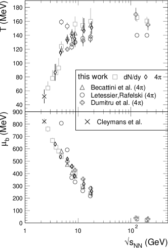
(a) Statistical Models

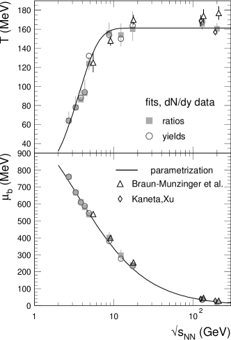
(b) Parametrization

Figure 8: 8(a) The chemical freeze-out temperature and baryon chemical potential (see text) of heavy ion collisions extracted using statistical models are shown as a function of collision energy. 8(b) The energy dependence is parametrized for the models described in [56]. Figures taken from [56].

The temperature and baryon chemical potential of heavy ion collisions, extracted using statistical models, is presented as a function of collision energy per nucleon pair in Fig. 8 [56]. The baryon chemical potential, $\mu_{B}$, is related to the net baryon density of the produced matter. It gives the amount by which the energy of the system would change if a baryon were added. In this way, it describes the tendency of the system to favor baryon production over antibaryon production; a system with more baryons than antibaryons would have a large $\mu_{B}$, as it would cost more energy to add a baryon than an antibaryon. The temperature at chemical freeze-out is seen to increase with collision energy sharply at first, and then very moderately for $\sqrt{s_{\scriptscriptstyle{{\rm NN}}}}\,{\buildrel>\over{{}_{\sim}}}\,10~{}\mbox{${\rm GeV}$}$, as shown in Fig. 8(b). The parameterizations used to fit the temperature and $\mu_{B}$ dependence are given in [56]. A limiting temperature of $161\pm 4~{}\mbox{${\rm MeV}$}$ was extracted from the fit. See [56] and [60] for a discussion of the energy dependence of the temperature extracted from statistical models.

3 Some Collision Models

As seen in Fig. 6 and 8, the matter produced in heavy ion collisions at high energy has a large energy density, low net baryon content and a high temperature compared to the matter produced in lower energy collisions. To learn more about this matter, it is necessary to have theoretical calculations of the collisions dynamics to which experimental results can be compared. Due to the difficulty of calculations in QCD, it is more practical to build a model from a set of coherent assumptions, which can be used to simulate the collision dynamics. Two such models were used for the analysis presented in this thesis.

The Heavy Ion Jet Interaction Generator (HIJING) [61] model is built upon the idea that in high energy heavy ion collisions, multiple minijet production will be important. A jet is a collection of closely correlated particles produced in elementary collisions [62]. The hadrons in a jet are thought to be generated from a single quark or gluon that was produced with a large transverse momentum. A minijet is a jet whose transverse momentum is not extremely large compared to the average $p_{\mathrm{T}}$ of produced particles. In the presence of a hot, dense medium, the width of a jet may be broadened, and a minijet may be completely absorbed [63]. HIJING can be used to test this idea, as it includes both minijet production and energy loss of particles in the produced medium. The production of low $p_{\mathrm{T}}$ particles, and the production of hadrons from quarks and gluons, are modeled via string breaking pictures (see Fig. 5). Some nuclear effects, such as shadowing [64], are also included.

The other collision simulation package used extensively in this analysis is known as A Multi-Phase Transport (AMPT) [65] model. This model uses HIJING to calculate the position and momentum of each parton (a parton is either a quark, antiquark or gluon) immediately following the collision. AMPT does not include the continuous minijet energy loss modeled in HIJING; instead AMPT models the individual re-scatterings of partons, using Zhang’s Parton Cascade (ZPC) [66] model. The partons are then hadronized using a modified version of the string fragmentation model in HIJING. Finally, interactions between hadrons are simulated using A Relativistic Transport (ART) [67] model, which is modified to include inelastic interactions between nucleons and antinucleons, as well as between kaons and antikaons.

4 Overview

Models such as HIJING and AMPT provide a phenomenological description of heavy ion collisions under a certain set of assumptions. How valid these assumptions are, and how accurate the descriptions turn out to be, can only be determined by observing nature. The PHOBOS experiment at the Relativistic Heavy Ion Collider (RHIC) used heavy ion collisions to shed light on the dynamics of strongly interacting matter under extreme conditions. It has been shown that this matter is both far more dense and far more hot than normal nuclear matter. The analysis presented in this thesis will examine the production of charged hadrons by both d+Au and nucleon-nucleus collisions, to serve as a reference for nucleus-nucleus interactions.

In the absence of any nuclear or produced medium effects, a nucleus-nucleus collision may be interpreted as a superposition of independent binary nucleon collisions. As will be discussed in Ch. 7, a significant suppression relative to binary collision scaling was observed in the high-$p_{\mathrm{T}}$ hadron production of central Au+Au collisions at $\sqrt{s_{\scriptscriptstyle{{\rm NN}}}}=200~{}{\mbox{${\rm GeV}$}}$. This result led to two competing hypothesis. One held that the initial nuclei were modified such that high-$p_{\mathrm{T}}$ hadron production was reduced. The other maintained that hadron production was unchanged, but that particles produced in the collision lose momentum as they travel through a dense, strongly interacting medium. These ideas were tested using d+Au interactions, which were expected to include any initial modification of the gold nucleus, but were not expected to produce a dense medium. The absence of any significant suppression of hadron production in d+Au interactions led to the acceptance of the hypothesis of partonic energy loss.

The analysis presented in this thesis will examine the validity of using d+Au collisions in place of nucleon-nucleus interactions as a reference for Au+Au. This study was performed by measuring the charged hadron spectra of d+Au, p+Au and n+Au collisions. The nucleon-nucleus interactions were extracted from the d+Au data by identifying the deuteron spectators. Two calorimeters were used to measure the deuteron spectators. One detected forward-going single neutrons and the other, installed just prior to the d+Au physics run at RHIC, detected forward-going single protons. It will be shown that the hadron production of p+Au and n+Au collisions can be combined to form an ideal reference for Au+Au interactions. In addition, the yield of positive and negative hadrons in p+Au collisions will be compared to that of n+Au. This comparison allows unique study of the ability of a nucleon-nucleus interaction to transport the initial “projectile” nucleon to mid-rapidity.

Finally, the hadron production of d+Au collisions will be examined as a function of centrality (i.e. impact parameter). Different measures of centrality will be employed, and the effects of centrality determination on the final measurement will be explored. These centrality measures will be used to study the shape of the charged hadron spectrum in d+Au collisions. As will be discussed in Sect. 3, the production of hadrons having a transverse momentum of $\sim 2.5~{}\mbox{${\rm GeV}$}$ is known to be enhanced in nucleon-nucleus collisions over nucleon-nucleon interactions. The centrality dependence of this enhancement will be studied, and an intriguing scaling behavior will be revealed.

Chapter 1 The PHOBOS Experiment

The analysis presented in this thesis used data obtained by the PHOBOS experiment. PHOBOS was one of four heavy ion experiments installed at the Relativistic Heavy Ion Collider (RHIC). It studied the strong interaction by observing nucleon-nucleon, nucleon-nucleus and nucleus-nucleus collisions. The collisions were provided by RHIC over a broad range of center-of-mass energies.

1 The Relativistic Heavy Ion Collider

The Relativistic Heavy Ion Collider (RHIC) at Brookhaven National Laboratory (BNL) was designed to collide heavy ions, primarily gold nuclei, at energies up to $200~{}\mbox{${\rm GeV}$}$ per nucleon pair in the center of mass frame ($\sqrt{s_{\scriptscriptstyle{{\rm NN}}}}$). Four experiments were built at RHIC to study collisions of nuclei: BRAHMS, PHENIX, PHOBOS and STAR. The BRAHMS experiment used its movable spectrometer arm to study particle production at different values of pseudorapidity. The PHENIX detector measured hadrons, photons and electrons and included two large muon hodoscopes. The STAR detector featured a large barrel Time Projection Chamber (TPC) in a solenoidal magnet which could observe almost all charged particles at mid-rapidity. The PHOBOS experiment is described in Sect. 2.

Generating collisions of heavy ions required sophisticated machinery to (a) produce ions by stripping electrons from atoms, (b) accelerate the ions to nearly the speed of light and (c) steer the beams of ions to cross paths and collide. RHIC made use of much of the existing accelerator infrastructure at BNL to strip electrons and accelerate ions. A new facility was constructed to complete the electron stripping, accelerate the ions to the final desired momentum and to collide the ion beams. A diagram of the complete RHIC facility can be seen in Fig. 1 [68].

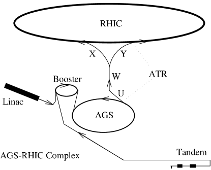
Figure 1: A schematic of the RHIC layout. $\mbox{Au}^{+77}$ ions exit the AGS at U, are stripped of electrons at W and $\mbox{Au}^{+79}$ ions are sent into two separate rings at X and Y [68].

Gold ions were first put into motion at the Tandem Van de Graaff accelerator. A pulsed sputter ion source produced gold ions with a net charge of negative one. The Tandem generated two static electric potential differences in sequence, one of $+15~{}{\mbox{${\rm MV}$}}$ and one of $-15~{}{\mbox{${\rm MV}$}}$. $\mbox{Au}^{-1}$ ions were first accelerated by the positive potential at the center of the machine and then passed through a thin foil which removed on average 13 electrons. The $\mbox{Au}^{+12}$ ions were then repelled and thereby accelerated by the positive potential and passed through another stripping foil.

Positively charged $\mbox{Au}^{+32}$ ions were then sent into the Alternating Gradient Synchrotron (AGS) complex. They were first accelerated by the Booster synchrotron from 1 ${\rm MeV}$ per nucleon up to 95 ${\rm MeV}$ per nucleon. As the ions exited the Booster, they were further stripped of electrons. $\mbox{Au}^{+77}$ then entered the AGS, where they were accelerated to RHIC injection energy of 10.8 ${\rm GeV}$ per nucleon. Beams were stored in the AGS until the RHIC rings could be filled. The ions were then stripped of the final two electrons, and $\mbox{Au}^{+79}$ ions entered the Relativistic Heavy Ion Collider.

To store two beams of positive ions, RHIC consisted of two independent rings. The rings had a circumference of 3.8 ${\rm km}$ and provided six interaction regions where the beams crossed. RHIC performed the final acceleration of the ions up to the full collision energy, a maximum of 100 ${\rm GeV}$ per nucleon for gold nuclei. At this energy, a magnetic field of 3.458 ${\rm T}$ was required to keep the ions traveling in a circle. This field was provided by superconducting dipole magnets, each of which was 9.46 ${\rm m}$ long and was cooled by liquid Helium to a temperature of 4.2 ${\rm K}$.

Particles in the beams traveled through the rings in bunches of $\sim 10^{9}$ ions. This allowed the bunches to be accelerated by successive “kicks” from radio-frequency electromagnetic fields. The longitudinal positions at which a bunch could ride the r.f. wave were referred to as buckets. Since not all buckets contained a bunch of ions, the RHIC facility kept track of which buckets were filled. A crossing clock was used to inform experiments of the times at which filled buckets would collide.

The beams were brought into alignment for collisions by two types of RHIC magnets, the D0 and DX dipoles. Four D0-magnets, two on each side of the Nominal Interaction Point (IP), brought the beams close enough that they could share a single beam pipe. The D0-magnets provided a field of 3.52 ${\rm T}$ for this purpose. The beams were then steered to collide by two DX-magnets, one on each side of the IP, each of which generated a field of 4.3 ${\rm T}$.

During the 2003 physics run, RHIC delivered deuteron-gold collisions with an integrated luminosity of 75 ${\rm nb}^{-1}$. The PHOBOS experiment recorded a total of 146 million d+Au collisions to tape. RHIC also provided Au+Au collisions at $\sqrt{s_{\scriptscriptstyle{{\rm NN}}}}=$19.6 ${\rm GeV}$, 55.9 ${\rm GeV}$, 62.4 ${\rm GeV}$, 130 ${\rm GeV}$ and 200 ${\rm GeV}$; polarized p+p collisions at $\sqrt{s_{\scriptscriptstyle{{\rm NN}}}}=$200 ${\rm GeV}$ and 410 ${\rm GeV}$; and Cu+Cu collisions at $\sqrt{s_{\scriptscriptstyle{{\rm NN}}}}=$22.5 ${\rm GeV}$, 62.4 ${\rm GeV}$ and 200 ${\rm GeV}$. The energy and species scans that RHIC provided were a striking display of the machine’s capabilities, and have been an invaluable source of information in the quest to understand how strongly interacting matter behaves under varying conditions. See [69] for an in-depth discussion of the RHIC facility.

2 PHOBOS Detector Setup

The PHOBOS experiment was designed to study global properties of the collisions and to search for previously unknown signals of new physics. These design goals established the need for several essential detector pieces. To observe global properties of collisions, a multiplicity detector array was constructed which could observe nearly all particles produced in a collision. To investigate the collision dynamics and search for signals of new physics, a two-arm spectrometer was assembled which could study a relatively small number of particles in great detail. To help determine the impact parameter of collisions, detectors were added to measure the amount of nuclear material which did not participate in the collision. Finally, to ensure that new and rare physics signals were not overlooked, a triggering and data acquisition system was built which could collect collision data at a high rate. A diagram of the PHOBOS detector used during deuteron-gold (d+Au) collision data taking is shown in Fig. 2.

Figure 2: The PHOBOS detector setup used to take deuteron-gold collision data. The proton calorimeters (see Sect. 3) are drawn to scale, but are located roughly 3 times further from the interaction point than shown.

1 The Multiplicity and Vertex Detectors

The PHOBOS multiplicity detector covered nearly the full 4$\pi$ solid angle. The bulk of produced particles were measured by the Octagon – a single layer of silicon pad sensors which form an octagonal barrel around the beam pipe. Particles emerging from the interaction point at very high pseudorapidity were measured by the Rings – six separate rings of silicon pad detectors oriented perpendicular to the beam. These detectors were used to count the number of produced particles, to classify collisions according to their centrality and to determine the collision vertex.

In addition to the silicon detectors described below, the PHOBOS experiment benefited greatly from its beam pipe. Of the four heavy ion experiments at RHIC, PHOBOS was unique in its use of 12 meters of beryllium beam pipe. Three sections of beryllium beam pipe were installed, each of which was 4 ${\rm m}$ in length, 76 ${\rm mm}$ in diameter and about 1 ${\rm mm}$ in thickness. The use of a thin beryllium pipe over the entire length of the PHOBOS multiplicity detector allowed a clean multiplicity measurement even at high values of pseudorapidity, where low particles with low transverse momentum would have been much more likely to scatter off of a steel beam pipe.

The Octagon

The Octagon was used to detect particles over a wide range of azimuthal angle and pseudorapidity values. It consisted of a light-weight aluminum frame which could support eight rows of up to thirteen silicon pad sensors. Each row of sensors formed one face of the octagonal barrel detector. In four of the faces, sensors were removed such that the acceptance of the Octagon did not overlap the acceptance of the Vertex or Spectrometer detectors. The Octagon was 1.1 ${\rm m}$ long with a diameter of 90 ${\rm mm}$ and could measure particles having pseudorapidity $\left|\eta\right|<3.2$ produced by collisions within 10 ${\rm cm}$ of the nominal interaction point. In addition to the silicon sensors themselves, the frame supported the electronics used to readout signals from the sensors, including a water cooling system that removed heat generated by the electronics.

All silicon sensors used in the Octagon were 84 ${\rm mm}$ long by 36 ${\rm mm}$ wide, with a grid of four by thirty active pads. Like all silicon sensors in PHOBOS, sensors in the Octagon had a thickness that was within 5% of 300 $\mu{\rm m}$. Each pad was 2.708 ${\rm mm}$ long (in the beam direction) and 8.710 ${\rm mm}$ wide. Despite the relatively large pads, sensors in the Octagon achieved a signal-to-noise ratio of $S/N\approx 13/1$. The Octagon is shown in Fig. 3 [70].

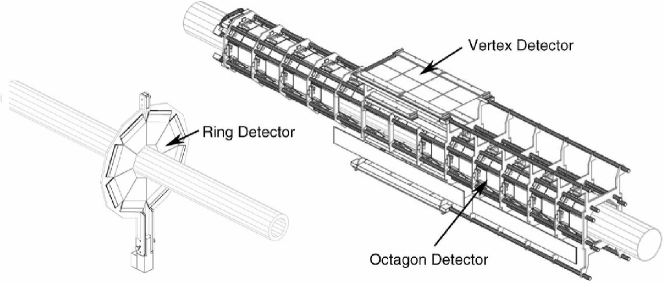
Figure 3: The PHOBOS silicon multiplicity detectors [70].

The Rings

Particles emitted at very forward angles were detected by the Rings. Each individual Ring was a set of eight trapezoidal silicon sensors, placed side-by-side to form a disk. The Rings were oriented transverse to the beam direction, so that the trajectory of particles with large longitudinal momentum would be nearly perpendicular to the face of the detector. The Rings and readout electronics were supported by carbon-fiber frames, to ensure that inactive material around the detectors was low-Z and would not be a large source of secondary particles. There were six Ring detectors in all, placed $\pm 1.13~{}\mbox{${\rm m}$}$, $\pm 2.35~{}\mbox{${\rm m}$}$ and $\pm 5.05~{}\mbox{${\rm m}$}$ from the IP. These detectors observed particles having pseudorapidity $3\leq\left|\eta\right|\leq 4$, $4\leq\left|\eta\right|\leq 4.7$ and $4.7\leq\left|\eta\right|\leq 5.4$, respectively. The inner radius of the Rings was 10 ${\rm cm}$, with each Ring sensor extending out 12 ${\rm cm}$ radially.

All silicon sensors used in the Rings had 64 active pads, arranged in eight radial rows and eight azimuthal columns. Unlike the rectangular sensors in other silicon detectors, pads in a single Ring sensor were not equally sized. Rather, each pad had the same acceptance in pseudorapidity, $\Delta\eta\approx 0.1$, and azimuth, $\Delta\phi\approx 2\pi/64$. Thus, pad sizes ranged from about 3.8 ${\rm mm}$ in the azimuthal direction by 5.1 ${\rm mm}$ in the radial direction for pads near the beam pipe, to about 10.2 ${\rm mm}$ by 10.2 ${\rm mm}$ for pads at the outer edge of the Ring. The average signal-to-noise ratio of Ring sensors was comparable to that of the Octagon. A diagram of a ring detector is shown in Fig. 3 [70].

Figure 4: The PHOBOS silicon detectors located close to the nominal interaction point. The top of the PHOBOS magnet has been removed to make the detector pieces visible [30].

The Vertex Detector

The Vertex detector was designed to provide accurate vertex resolution, better than 0.2 ${\rm mm}$ along the beam direction for collisions within 10 ${\rm cm}$ of the IP, in the high-multiplicity environment of a central Au+Au collision. To achieve this, two double-layer detectors were constructed, one placed above the beam line and one below, both centered around the nominal interaction point. This arrangement allowed the collision position to be reconstructed by identifying two-point tracks that point to a common vertex in each of the double-layer detectors. While this was the preferred method for Au+Au collisions, in low-multiplicity environments such as d+Au, a different vertex reconstruction method was used (see Sect. 2).

Two types of silicon sensors were used in the Vertex detector. The layers closest to the beam line (56 ${\rm mm}$ in the vertical direction), known as the Inner Vertex, consisted of four sensors placed side-by-side in the beam direction. Each sensor had a grid of 128 pads in the beam direction by 4 pads in the transverse direction. Pads in the Inner Vertex were 0.473 ${\rm mm}$ long in the beam direction and 12.035 ${\rm mm}$ wide. The layers further from the beam line (118 ${\rm mm}$ in the vertical direction), known as the Outer Vertex, consisted of two rows of sensors, each row having four sensors placed side-by-side in the beam direction. Each of these sensors had a grid of 128 pads in the beam direction by 2 pads in the transverse direction. Pads in the Outer Vertex were 0.473 ${\rm mm}$ long in the beam direction and 24.070 ${\rm mm}$ wide. Sensors in the Vertex detector achieved a better signal-to-noise ratio than those in the Octagon or Rings. The top Outer Vertex can be seen in Fig. 3 [70].

2 The Spectrometer Detectors

Whereas the multiplicity and vertex detectors were used to observe the bulk of particles produced in a collision, PHOBOS employed its spectrometer to study in detail a small number of produced particles. Particle momentum was determined by tracking the particle’s motion through a magnetic field. Tracking was performed using a two-arm silicon pad spectrometer that was situated in a 2 T magnetic field. Particle mass could then be determined using energy loss in the silicon and/or time-of-flight information. A Time-of-Flight (TOF) wall was used to obtain the particle’s speed.

The PHOBOS Magnet

The PHOBOS magnet made it possible to identify the sign of the electric charge and the momentum of particles produced near mid-rapidity. For purposes of particle tracking, it was desirable to have a low-field region close to the interaction and a high-field region further from the collision. Particle trajectories in the low-field region were essentially straight. These straight tracks were used as seeds from which the full path taken by a particle through the high-field region could be reconstructed. In addition, a near-zero field very close to the beam helped to ensure stable storage of the beams inside the collider.

Such a field was achieved by a double-dipole magnet that functioned at room temperature [71]. The two dipole fields were produced using four copper coils, two just above each Spectrometer arm and two just below. The vertical gap between the pole tips, into which the Spectrometer was placed, was 158 ${\rm mm}$ when the magnet was off. The four coils were of cylindrical “double-taper” design, but with two cuts to provide the desired field shape. One cut was vertical and one was at 12^∘ to vertical. The coils were supported by a steel flux return yoke, two pole support plates, four support columns and an adjustable magnet stand. Under full power and full magnetic field, the yoke deflection was about 2 ${\rm mm}$. The physical design of the PHOBOS magnet is shown in Fig. 5(a).

The coils were energized using a refurbished AGS power supply that provided up to 3600 ${\rm A}$ at 115 ${\rm VDC}$. The coils were driven in a series-parallel configuration, with the top two coils in one series electrical circuit and the bottom two coils in another circuit. This produced two dipole fields with opposite polarity. The voltage drop across each coil was $0.0264~{}\Omega\times 1800~{}\mbox{${\rm A}$}=47.5~{}\mbox{${\rm V}$}$, so the total voltage drop for the series circuit was 95 ${\rm V}$. Heat generated by resistance in the conductors was dissipated by water cooling. The maximum field strength in the vertical direction was 2.18 ${\rm T}$, while the field components in the two horizontal directions were less than 0.05 ${\rm T}$. A map of the vertical field strength is shown in Fig. 5(b). It was possible to invert the vertical component of the magnet field by reversing the flow of electric current through the coils. The field orientation was said to be positive, “B$+$,” when the field covering the outer-ring Spectrometer arm was directed upward. This is the orientation shown in Fig. 5(b). During data taking, PHOBOS attempted to record an equal number of collisions with each magnet polarity.

(a) Physical Magnet

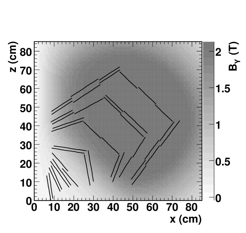
(b) Magnetic Field

Figure 5: The PHOBOS magnet. 5(a) A picture of the magnet before installation. 5(b) The vertical component of one of the dipole fields, with Spectrometer shown, as viewed from the bottom-up.

The Silicon Spectrometer

The motion of particles produced near mid-rapidity was tracked by the Spectrometer, a two-arm silicon pad detector. The spectrometer arms were centered on the beam line vertically, located on opposite sides of the beam and supported inside the PHOBOS magnetic field (see Sect. 2). Each spectrometer arm consisted of 16 layers of silicon sensors, as shown in Fig. 4 [30]. The arms were not centered at mid-rapidity, but rather extended slightly forward. Sensor layers in the Spectrometer were mounted on aluminum frames which were themselves mounted on large carrier plates. The carbon-epoxy carrier plates were designed to minimize vibrations caused by changes in the magnet current. These plates were supported on rails, allowing the Spectrometer arms to be mounted outside the magnet and then slid into place.

The Spectrometer contained five different types of silicon sensors. Sensors positioned closest to the interaction were the most finely-grained sensors; in general, pad size increased as distance from the interaction became greater. This strategy was employed to reduce the cost (and difficulty) of silicon production at the expense of decreased resolution in the particle’s azimuthal angle. Details on the size and placement of each sensor type used in the Spectrometer can be found in Table 1. Spacial positions of the sensors are presented in Fig. 6. The horizontal width of pads in type 2 sensors are smaller than those in type 1 sensors to make it possible to detect small deflections in particle trajectory when entering the non-zero region of the magnetic field. The width of pads in sensor types 3-5 are smaller than those in type 1 to improve momentum resolution.

Sensor Type	Number of Pads	Pad Size	Sensor Placement
	(horiz.$\times$vert.)	(${\rm mm}$$\times$${\rm mm}$)	(layers)
1	$70\times 22$	$1.000\times 1.0$	1-4
2	$100\times 5$	$0.427\times 6.0$	5-8
3	$64\times 8$	$0.667\times 7.5$	9-16, near beam
4	$64\times 4$	$0.667\times 15.0$	9-12
5	$64\times 4$	$0.667\times 19.0$	13-16

Table 1: Physical description of silicon sensors in the Spectrometer.

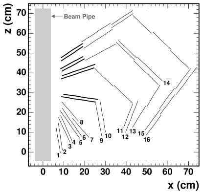
Figure 6: Location of sensors in one arm of the PHOBOS spectrometer, as viewed from the bottom-up. Layers are labeled by number and type 3 sensors are shown with thick lines.

The Time-of-Flight Wall

PHOBOS used a Time-of-Flight (TOF) wall composed of two sections to extend its particle identification capability. Each section of the wall consisted of 120 scintillators, giving the complete wall a pseudorapidity coverage of $0<\eta<1.24$. As the wall was located on the inner-ring side of the beam, particle identification using the TOF wall was only possible for particles passing through the corresponding spectrometer arm. Prior to the d+Au physics run, the TOF wall was moved away from the beam as far as possible, to extend particle identification capabilities for particles with higher transverse momentum. A schematic of one TOF wall is shown in Fig. 7 [70].

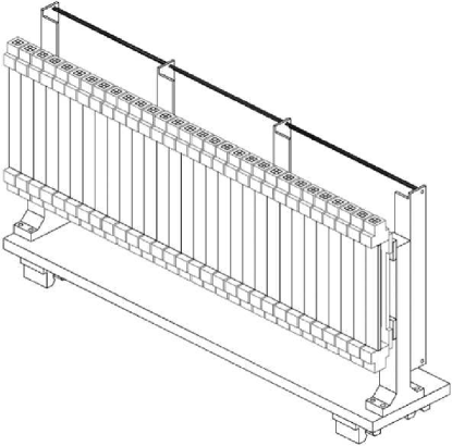
Figure 7: The physical layout of one TOF wall [70].

The scintillator material was chosen to have good timing (1.8 ${\rm ns}$ decay constant), a reasonable attenuation length (8 times the scintillator length) and an emission wavelength (408 ${\rm nm}$) that would ensure good response from the Photomultiplier Tubes. Each scintillator had a cross sectional area of $8~{}\mbox{${\rm mm}$}\times 8~{}\mbox{${\rm mm}$}$ and a height of 200 ${\rm mm}$. Scintillator light was detected by PMTs with a fast rise time of 1.8 ${\rm ns}$ and a high gain of $10^{6}$. Anode signals from the PMTs were split; one signal was sent to a leading-edge discriminator located close to the tubes while the other was sent to an Analog-to-Digital Converter (ADC) module after passing through a 400 ${\rm ns}$ delay cable. The discriminator signal was sent to a Time-to-Digital Converter (TDC) module that featured a sensitivity of 25 ${\rm ps}$ per digital channel. Pulse height and timing information were used together to perform slewing corrections and improve the overall timing resolution of the TOF wall.

The PMTs were attached at both the top and bottom of the TOF wall, which allowed the vertical position at which a particle struck the wall to be determined. The position resolution, as measured using cosmic rays and radioactive sources, was found to be 10 ${\rm mm}$ for reconstruction based on time difference and 37 ${\rm mm}$ for reconstruction based on the ratio of pulse heights. Timing resolution for the TOF wall in data was better than 100 ${\rm ps}$.

3 The Calorimeters

Since nuclear collisions in the collider occurred with varying impact parameter, it was necessary to have physical observables which were correlated with the impact parameter of a collision. The number of nucleons leaving the collision with near-beam rapidity is an example of one such observable, since such nucleons should not have directly participated in the collision. PHOBOS measured the energy, rather than the number, of such nucleons. The energy of these spectator neutrons was measured using the Zero-Degree Calorimeter (ZDC). The energy of spectator protons was measured using the Proton Calorimeter (PCAL).

The Zero-Degree Calorimeters

The Zero-Degree Calorimeter (ZDC) detectors were used to detect free neutrons (those not bound in a nuclear fragment such as an alpha particle) emerging from a collision with near-beam rapidity. While such neutrons were not deflected by the collision itself, their trajectories could be affected by the breakup of the nucleus. At RHIC, such evaporation neutrons diverged from the beam axis by less than 2 ${\rm mrad}$. The ZDCs were 10 ${\rm cm}$ wide and located roughly 18 ${\rm m}$ from the IP, so that they covered a horizontal deflection of about $2.7~{}\mbox{${\rm mrad}$}$. There were two ZDCs, one on each side of the collision. Each calorimeter consisted of 3 ZDC modules.

The RHIC accelerator magnets were exploited to remove all charged particles from the acceptance of the ZDC. As the beams emerged from the interaction region, they passed through the RHIC DX-magnets, which were used to bend the two beams back into their separate pipes. These magnets have the desirable side-effect of causing the region between the RHIC beam pipes, past the DX-magnets, to be inaccessible to charged particles emerging from the interaction region. The ZDC detectors were placed in this “zero-degree” region, where any produced or secondary particles would deposit negligible energy compared to that of spectator neutrons. The design of the ZDC modules was restricted by the space limitations imposed by their position in the experiment. See Fig. 8 [72] for a schematic of the ZDC positioning and the paths taken by charged particles through the DX-magnets.

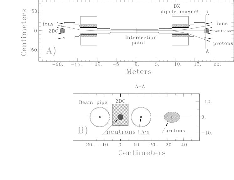
Figure 8: Bird’s-eye view (top) and “beam’s-eye” view (bottom) of the collision region, showing the location of the ZDCs and the paths taken by gold ions, protons and neutrons [72].

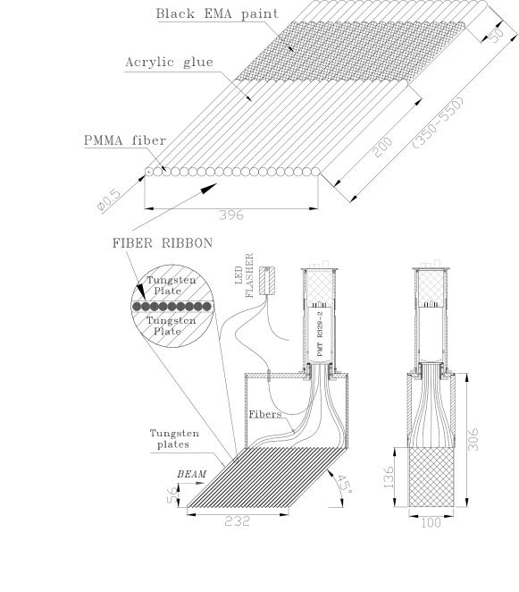
Figure 9: Construction design of a ZDC module. Dimensions shown are in millimeters [72].

The calorimeters were designed to minimize the loss in energy resolution due to shower leakage. They were not designed to provide information about the transverse position of the neutrons. The ZDCs did not use scintillating material to generate light, rather optical fibers were employed in which shower secondaries produced Čerenkov light. Early simulations had shown that a detector using Čerenkov light could observe more of the shower signal than a detector using scintillator. Each ZDC module consisted of optical fibers sandwiched between 27 Tungsten alloy plates, with each plate having dimensions of $100~{}\mbox{${\rm mm}$}\times 187~{}\mbox{${\rm mm}$}\times 5~{}\mbox{${\rm mm}$}$. Tungsten alloy was chosen as the stopping material since simulations showed that it allowed more of the shower signal to be detected than Lead would have. The plates were oriented 45^∘ from vertical, to roughly coincide with the Čerenkov angle of light emitted by particles going near the speed of light in the fibers. The Čerenkov light from one module was detected by a single photomultiplier tube, which gave both signal strength and timing information. The energy resolution of a full ZDC (3 modules) was found to be $\sigma_{E}/E=19\%$ and the timing resolution was found to be better than 200 ${\rm ps}$. The timing resolution was sufficient to allow these detectors to be used as a minimum bias collision trigger during Au+Au physics runs. A diagram of the ZDC construction is shown in Fig. 9 [72].

The Proton Calorimeters

Before the d+Au physics run, PHOBOS installed additional calorimeters to compliment and extend its ability to measure forward-going nuclear fragments. Whereas the ZDC detectors collected energy from spectator neutrons, the Proton Calorimeter (PCAL) detectors measured the energy of free spectator protons. The PCAL detectors were not symmetric during the d+Au run; a large calorimeter was installed on the Au-exit side of the interaction region and a small calorimeter was placed on the d-exit side. The Proton Calorimeter on the Au-exit side (Au-PCAL) was used for obtaining a measurement of collision centrality, while the Proton Calorimeter on the d-exit side (d-PCAL) was used to identify collisions in which the proton from the deuteron did not participate. A large fraction of the design and assembly of the PCAL detectors as well as the entirety of the commissioning, monitoring, calibration (see Sect. 3), and analysis (see Ch. 3 and 5) was completed as part of this thesis work.

Like the ZDCs, the PCAL detectors also exploited the RHIC DX-magnets. These magnets were designed to bend beams of gold nuclei into their separate beam pipes. Since a gold nucleus has a rigidity of $Z/A=79/197=0.4$, while a single proton has a rigidity of 1, the DX-magnets deflected beam-rapidity protons twice as much as they deflected gold nuclei. This extra deflection was sufficient to kick protons completely out of the RHIC beam pipes and into the Au-PCAL. See Fig. 10(b) for a comparison of the paths taken by gold nuclei and protons. A similar situation occurred on the deuteron-exit side of the interaction, since a deuteron has a rigidity of 0.5, comparable to that of a gold nucleus. The rough equivalence in rigidity was a major motivation for RHIC to perform d+Au collisions rather than p+Au.

(a) Physical Layout

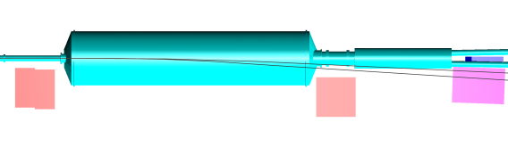
(b) Proton Trajectories

Figure 10: Top views of the PHOBOS Proton Calorimeter. 10(a) The physical location of the PCAL. The PCAL Shielding and the ZDC are not shown. 10(b) The black lines show the paths taken by 100 GeV$\kern-1.49994pt/\kern-1.19995ptc$ and 50 GeV$\kern-1.49994pt/\kern-1.19995ptc$ protons as they are bent by the DX Magnet. Also shown are the PCAL Shielding blocks and the ZDC.

The PCAL detectors were constructed using lead-scintillator hadronic calorimeter modules that had originally been assembled for the E864 experiment at the AGS [73]. Each module consisted of a lead-scintillator brick 117.0 ${\rm cm}$ in length with a square cross-section of 10 ${\rm cm}$ on each side. An array of $47\times 47$ scintillator fibers was contained in each module. The lead-scintillator bricks were constructed by rolling thin sheets of lead (with a 1% antimony admixture) through a grooving machine, laminating the sheet and then manually placing a ribbon of 47 scintillator fibers into the grooves. This process was then repeated 46 times to complete a module, and more than 750 modules were constructed for use in the E864 experiment. Great care was taken to ensure precise uniformity in the inter-module fiber lattice. Attached to the brick section was an ultra-violet absorbing Lucite light guide, that ensured clean transmission of scintillation light ($\lambda=435~{}\mbox{${\rm nm}$}$) without contamination from any Čerenkov radiation created in the light guide. See  Fig. 11 [74] for a diagram of a PCAL module.

Figure 11: Design of a PCAL module. The inset shows the spacing of scintillator fibers [74].

Since the decommissioning of the original E864 calorimeter was not an easy process – the modules had been freshly painted before assembly and had since stuck together – and because the modules had been stored outside, careful testing of modules was necessary before they could be used in PHOBOS. Testing was performed using cosmic rays. After the decommissioning of E864, the modules had been cleverly stacked in rows of ten, six layers high. Alternating layers were oriented at right angles. Thus it was possible to use modules from three layers as cosmic ray triggers to test both the response and attenuation length of modules in the remaining three layers. Since PMTs were also salvaged from the original E864 equipment, these tubes were tested at the same time as the modules. For purposes of building the PCAL detectors, modules with better attenuation lengths and PMTs with desirable gains were placed in the region of the detector expected to contain most of the shower signal.

Assembly of the PCAL detectors was complicated by the weight of the modules, about 100 ${\rm kg}$, and by their fragility. In addition to the softness of the lead and the possibility of breaking some of the scintillator fibers, light guide detachment was a common problem. As a result of testing and handling, more than 10% of modules were rejected. After having passed testing and visual inspection (to reject modules which had bowed), modules were placed into a specially designed, light-tight aluminum box. Mounting the modules onto the table of the box presented its own challenge. Since the PCALs were positioned on the outer-ring side of the beam, and since there was no direct access to that side of the RHIC tunnel, the calorimeters had to be assembled in the experimental area – the full calorimeter was too big and too heavy to be transported above or below the beam pipes. The modules were mounted using a manually operated chain hoist that had been installed at the proper location in the RHIC tunnel for a different purpose (to transport accelerator power supplies). As the shape of each module had warped to some extent, great care was taken to ensure that the modules were spaced uniformly in both the horizontal and vertical direction. Uniformity was further necessitated by the back plate of the Au-PCAL box: an inch-thick aluminum plate with a grid of $9\times 12$ conical holes through which the ends of all light guides were required to pass. The Au-PCAL detector consisted of an array 8 modules wide and 10 modules high. On top of this array was one row of 7 modules, with the “missing” module away from the beam line. Two more modules were then added to this row, one near the beam line and one away. These modules were used to provide extra support for the top of the calorimeter box. Light absorbing filters were then added to the PMTs of two modules, see Sect. 3.

Figure 12: A photograph of the fully commissioned Au-PCAL. Easily seen are the PMT mountings and readout cables. To guide the eye, certain features have been labeled: the cosmic ray trigger modules (T1-T4), the shielding (Shld) and the D0-magnet (D0). During normal operation, the Kevlar tarp covered the full box, to help prevent light-leaks.

Assembly of the small d-PCAL, used only during the d+Au physics run, was far more simple. This calorimeter consisted of only four modules, individually wrapped in Kevlar for light-tightness and to contain any lead-oxide, resting on an open table adjacent to the beam pipe. After the d+Au physics run, the small d-PCAL was replaced with a full sized calorimeter. Both full sized calorimeters had Kevlar-wrapped modules placed outside, above and below, the calorimeter boxes to be used as cosmic ray triggers. An assembled calorimeter is shown in Fig. 12.

Shielding for the Proton Calorimeters

Shielding was installed to block produced particles from depositing energy into the PCAL detectors. While the ZDCs were inaccessible to produced particles due to their extreme forward position, the Au-PCAL covered a pseudorapidity region of roughly $-3.6<\eta<-5.2$. Two shields were constructed, each using four blocks of high-density (4.0 ${\rm gm}/{\rm cm}^{3}$) concrete. The blocks measured $88.9~{}\mbox{${\rm cm}$}\times 44.45~{}\mbox{${\rm cm}$}\times 44.45~{}\mbox{${\rm cm}$}$ and were positioned roughly at beam height. One shield was placed about 8 ${\rm m}$ from the IP and moved as close to the beam as possible (about 20 ${\rm cm}$). The other shield was situated near the calorimeter, almost 15 ${\rm m}$ from the IP and was positioned roughly 40 ${\rm cm}$ from the beam line, to allow spectator protons to reach the calorimeter without being blocked by the shielding. Simulations of these shielding blocks showed that even 50 ${\rm GeV}$ pions (protons) would deposit less than 5% (2.5%) of their energy into the calorimeter. The shield positions can be seen in Fig. 10(b).

4 The Trigger Detectors

PHOBOS used several different detectors to determine that a collision with various properties had occurred in the experiment. For high multiplicity Au+Au collisions, the Paddles served as the primary event trigger while the Čerenkov counters could be used to trigger on the collision vertex. Before the d+Au physics run, two more trigger detectors were installed – the Time-Zero Counters and the Spectrometer Trigger (SpecTrig). The T0s were used to provide a more accurate vertex and collision time than the Čerenkov counters could provide. The SpecTrig provided a trigger for collisions producing a high-$p_{\mathrm{T}}$ particle in one arm of the Spectrometer.

The Paddle Counters

The Paddle counters were used during Au+Au physics runs both to trigger on collisions and to determine centrality. There were two Paddle counters, each consisting of a circular array of 16 plastic scintillators, positioned $\pm 3.21~{}\mbox{${\rm m}$}$ from the nominal interaction point. This position gave them a pseudorapidity coverage of $3<\left|\eta\right|<4.5$. Plastic scintillator was chosen for its good timing resolution (150 ${\rm ps}$), large dynamic range (from 1 Minimum Ionizing Particle (MIP) up to 50 per collision) and high tolerance of radiation. A diagram of a Paddle counter is shown in Fig. 13 [75].

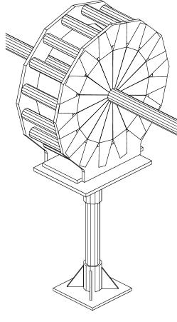
Figure 13: Schematic diagram of a Paddle counter [75].

Individual scintillators were 18.6 ${\rm cm}$ long, 0.85 ${\rm cm}$ thick, 1.9 ${\rm cm}$ wide at the inner edge and 9.5 ${\rm cm}$ wide at the outer edge. Attached to the scintillator was a two-component acrylic light guide. While the scintillator was oriented transverse to the beam, the PMTs were oriented longitudinally. This arrangement was achieved by coupling one section of the light guide to the scintillator, one section to the photomultiplier tube and using a 45^∘ Aluminized mirror between the light guide components. Both amplitude and timing information was available from the Paddle signals. The full Paddle counters performed with a time resolution of about 1 ${\rm ns}$, an energy resolution of $\sigma_{E}/\Delta E=45\%$ for a single MIP, a signal-to-noise ratio of about 20/1 and a triggering efficiency of 100% for central and semi-peripheral Au+Au collisions.

The Čerenkov Counters

The Čerenkov counters were used to provide real-time collision vertex information. There were two Čerenkov detectors, each consisting of 16 modules, placed $\pm 5.5~{}\mbox{${\rm m}$}$ from the IP. The radiators circled the beam pipe at a radius of 8.57 ${\rm cm}$ and were oriented longitudinally to the beam. Their positioning covered 37% of the solid angle in the pseudorapidity range $4.5<\left|\eta\right|<4.7$. See Fig. 14 [76] for a diagram of a Čerenkov detector.

Individual Čerenkov radiators were made of acrylic (the same type used as a light guide for the Paddles) in the shape of a cylinder with a 4.0 ${\rm cm}$ length and a 2.5 ${\rm cm}$ diameter. No light guide was necessary; PMTs were attached to the radiators with silicon elastomer. The modules were mounted in a mechanical structure that allowed individual modules to be moved within a 100 ${\rm mm}$ range in the beam direction. This allowed individual counters from each side of the interaction to be matched to within 50 ${\rm ps}$. The total timing resolution achieved by the Čerenkov counters was 380 ${\rm ps}$.

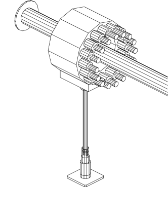
Figure 14: Schematic diagram of a Čerenkov detector [76].

The Time-Zero Counters

Prior to the d+Au physics run, Time-Zero Counters (T0s) were installed. These detectors were used to obtain accurate time-zero information and could be moved to a region of pseudorapidity appropriate for a d+Au collision. There were two T0s, each consisting of 10 modules arranged in a circle of 151 ${\rm mm}$ in diameter about the beam pipe. One of the T0s was located 2.6 ${\rm m}$ from the IP on the deuteron exit-side of the collision and the other was located 5.4 ${\rm m}$ from the IP on the gold exit-side of the collision. These locations were not fixed – for p+p collisions, for example, each module was moved closer to the IP. At their d+Au physics running positions, the T0s had a pseudorapidity acceptance of $3.7<\eta<4.2$ (d-side) and $-4.9<\eta<-4.4$ (Au-side).

Acrylic Čerenkov radiators were also used for the T0s. While the type of radiator was the same as that used for the Čerenkov counters, the type of PMTs was not. The PMTs used for the T0s had a rise time that was twice as fast as those used for the Čerenkov counters. The shape of the radiators used for the T0s also differed from those used in the Čerenkov counters. Radiators in the T0s had a diameter of 50 ${\rm mm}$ and a length of 25 ${\rm mm}$. Their acceptance, mobility and response time made the T0s the preferred detector for determining time-zero and for obtaining real-time vertex information for use in collision triggers.

The Spectrometer Trigger

The Spectrometer Trigger (SpecTrig) was commissioned for use in the d+Au physics run. It consisted of two walls of plastic scintillators, each containing 10 modules, and was designed to have an acceptance which covered that of the TOF. Each scintillator module was 11 ${\rm cm}$ long vertically, 7.24 ${\rm cm}$ wide horizontally and 0.5 ${\rm cm}$ thick. The scintillators were connected to trapezoidal light guides, that were then glued to PMTs using optical cement. The SpecTrig modules were mounted on an aluminum frame that was then attached to the PHOBOS magnet yoke.

This trigger was used in low-multiplicity environments (d+Au and p+p) for the real-time selection of events containing a particle with high transverse momentum that could be tracked using the Spectrometer and TOF. The selection was provided by combining real-time vertex information from the T0s with the position of hits in the SpecTrig and TOF walls. For particles with large transverse momentum ($p_{T}\,{\buildrel>\over{{}_{\sim}}}\,2~{}\mbox{\rm GeV$\kern-1.49994pt/\kern-1.19995ptc$}$), these three positions should fall on a single line. Thus, the trigger selected collisions for which some combination of a hit in the SpecTrig and a hit in the TOF formed a line that pointed back to the vertex position provided by the T0s. This trigger could only function when the occupancy of the SpecTrig and TOF walls were low, so that random combinations of hits from different particles were not likely to be collinear with the collision vertex.

5 The Data Acquisition

Once signals from the trigger detectors had been digitized, a decision could be made regarding whether or not to record the full PHOBOS detector state to disk. A description of the digitizing process for silicon signals can be found in Sect. 1, while descriptions of the various trigger criteria can be found in Sect. 1. During the d+Au physics run, the PHOBOS Data Acquisition (DAQ) system was used to process signals from over 135,000 silicon channels and 1,500 photo-tube channels at a rate of up to 280 events per second. The DAQ resided in a single VERSAmodule Eurocard (VME) crate and consisted of a 22-node computing farm to process the data, a computer module to assemble the processed data into an event, a disk array for temporary data storage, a module to monitor trigger signals and server to ship the processed data to tape storage [77].

The RACEway computing farm that processed the data was provided by Mercury Computer Systems, Inc. Each node had a 300 ${\rm MHz}$ PowerPC-750 processor with 1 ${\rm MB}$ of Level 2 (L2) Static Random Access Memory (SRAM) cache and 32 ${\rm MB}$ of Dynamic Random Access Memory (DRAM) memory. The computing farm was mainly used to check the data for consistency and to compress the silicon data. Because it was necessary to make offline corrections for common-mode noise and crosstalk among silicon channels, signals from empty channels needed to be preserved. This was done by first subtracting the known pedestals and then using lossless Huffman compression, which encoded the most frequently occurring ADC samples into short bit patterns. A compression factor of 3.5 was achieved for Au+Au collision data.

After processing, the data was sent to the event builder through a Front Panel Data Port (FPDP) connection at a rate of 43 ${\rm MB/s}$. The event builder used synchronization tags, which had been applied to each worker’s data block when the trigger signal was received, to assemble a complete event. The event was then stored in memory until it could be written to the disk cache. Files of roughly 1 ${\rm GB}$ in size (over 10,000 d+Au events) were shipped to the High Performance Storage System (HPSS) at the RHIC Computing Facility (RCF) over a Gigabit Ethernet connection. While the PHOBOS DAQ disk cache could write events at a rate of 50 ${\rm MB/s}$, simultaneous writing and reading resulted in a writing speed of 28 ${\rm MB/s}$ and a sustained throughput to HPSS of 30 ${\rm MB/s}$.

Chapter 2 Detector Calibration

All detectors in PHOBOS reported their measurements through various electronic read-outs. Once these raw signals had been recorded, several steps were required to determine the physical properties of the particles that produced them. The first step was to determine the amount of energy the particle had deposited into the detector as it passed through.

1 Silicon Signal Processing

The purpose of a PHOBOS Silicon detector was to measure both the position at which particles passed through the detector as well as the amount of energy they deposited in doing so. This information was obtained by correcting the raw signal for (a) an overall offset, (b) fluctuations in the read-out electronics, (c) the amount it had been amplified and (d) the possibility that the deposited energy was not due to a particle traveling transverse to the detector plane.

1 Semiconductor Detectors

As charged particles pass through a semiconductor material, electromagnetic collisions excite electrons out of the valence energy band of the crystal, leaving behind an effective positively charged hole. The goal of such a detector is to measure the number of electron-hole pairs created due to the ionizing particle. This information can then be related back to the amount of energy the particle deposited into the detector.

Silicon semiconductor devices are desirable due to the small amount of energy ($\approx 1~{}\mbox{${\rm eV}$}$) required to excite an electron from the valence to the conduction band. This allows an ionizing particle to create a large number of electron-hole pairs, which in turn allows for a precision measurement to be made of the deposited energy. However, the gap between the valence and conduction bands is so small that, at finite temperatures, thermal energy is sufficient to create electron-hole pairs. These electron-hole pairs lead to a current through the semiconductor, even in the absence of an ionizing particle. The ideal semiconductor detector would be a material which could freely conduct any electron-hole pairs produced by an ionizing particle, but would have no such leakage current. While the ideal situation cannot be realized, the leakage current of semiconductor detectors is minimized by creating a large insulating region in the material known as a depletion region.

A depletion region arises when a crystal with an excess of electrons above the valence band is brought into equilibrium with a crystal that has an excess of holes above the valence band. Such materials are obtained by doping a semiconductor with impurities. When the dopant atom has more electrons than the base semiconductor atoms, the resulting crystal has an energy level between the valence and conduction bands in which the extra electrons would sit at zero-temperature. At room temperatures, on the other hand, nearly all of the electrons in this energy band are excited into the conduction band by thermal energy. However, these electrons do not leave a hole in the lattice, so such doped crystals have an excess of negative charge carriers and are thus known as n-type doped semiconductors. Similarly, p-type doped semiconductors are those which have an excess of positive charge carries (holes) resulting from dopant atoms that have fewer electrons than the base semiconductor. A p-n junction is formed when an n-type semiconductor is brought in contact with a p-type semiconductor. Excess electrons in the n-type material are attracted to the excess holes in the p-type material, resulting in a current across the junction. As electrons fall into holes and become stuck at crystal lattice points, the dopant atoms are left lacking an electron (or hole) and become exposed charged ions. The charged ions create an electric potential that is positive on the n-type side of the junction and negative on the p-type side. This potential tends to prevent the flow of charges and allows the material to reach equilibrium. The region at the junction is thus a good region for detecting ionizing particles: it has effectively no leakage current but would conduct excited charge carriers. The extent of this depletion region can be increased by applying an external electric field across the junction to increase the potential in the n-type side. This is known as reverse-biasing the p-n junction. For more information on semiconductor detectors, see [78].

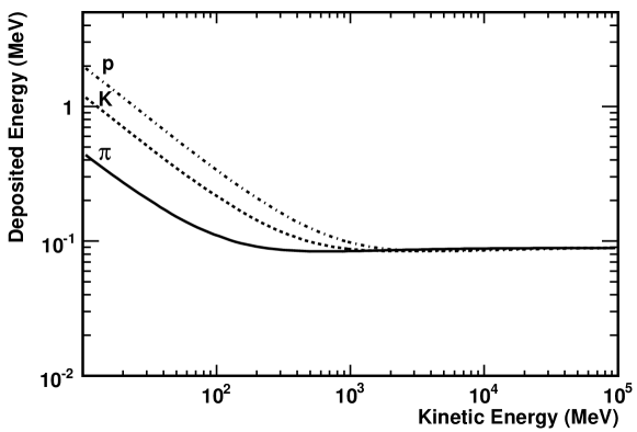
Figure 1: The average amount of energy deposited by pions, kaons and protons into 300 $\mu{\rm m}$ of silicon.

The average amount of energy an ionizing particle loses as it travels through material can be estimated using the Bethe-Bloch formula. This formula has the form

$$-\frac{\mathit{dE}}{\mathit{dx}}=(0.1535~{}{\mbox{${\rm MeV}$}{\mbox{${\rm cm}$}^{2}}/\mbox{${\rm g}$}})~{}\rho\frac{Z}{A}\frac{z^{2}}{\beta^{2}}\left[\ln\left(\frac{2m_{e}\gamma^{2}\beta^{2}c^{2}W_{\rm max}}{I^{2}}\right)-2\beta^{2}\right]$$ (1)

where $\rho$ is the density of the material in ${\rm gm}/{\rm cm}^{3}$, $Z$ is the atomic number of the material, $A$ is the atomic weight of the material in a.u., $m_{e}$ is the mass of the electron (0.511 MeV$\kern-1.49994pt/\kern-1.19995ptc^{2}$), $z$ is the charge of the ionizing particle in units of $e$, $\beta$ is the speed of the particle in units of $c$, $\gamma=1/\sqrt{1-\beta^{2}}$, $W_{\rm max}$ is the maximum energy transfer in a single collision and $I$ is the average energy required to excite a bound electron from an atom in the material. Discussions of this equation and common corrections to the energy loss formula can be found in the literature, see for example [79]. The average amount of energy deposited by several different types of particles in a typical PHOBOS Silicon detector is shown in Fig. 1. Notice that the minimum amount of energy deposited by pions, kaons and protons is roughly equivalent. Particles depositing this minimum amount of energy are known as Minimum Ionizing Particles (MIPs).

MIPs are important in high-energy physics, since most of the particles produced in a collision will deposit nearly the minimum amount of energy into a detector. For a very thick detector, an ionizing particle would experience a very large number of roughly independent collisions, while losing a negligible amount of energy in each collision. After measuring many ionizing particles, the distribution of energy deposited into the thick detector by the particles would be a Gaussian whose mean was equivalent to the energy deposited by one MIP. For a thin detector, such as the Silicon detectors used in PHOBOS, the number of collisions would be much smaller. The energy distribution observed by such a detector would not be Gaussian, but would have a high-energy tail due to (rare) Collins in which the ionizing particle loses a significant amount of energy. This distribution is known as a Landau; examples can be seen in Fig. 3 and 5.

2 The PHOBOS Silicon Read-out

PHOBOS Silicon detectors were constructed using a ($\approx 300~{}\mbox{$\mu{\rm m}$}$) thick n-type layer of silicon, with p-type silicon read-out pads. The pads were reverse-biased by applying positive voltage to the back plane of the n-type wafer and grounding the p-type pad via a $5.5\pm 0.2~{}\mbox{${\rm M}\Omega$}$ resistor. This design was based on the silicon detectors developed for the WA98 experiment [80]. While the reverse-biasing voltage served to create the depletion region, it also pulled apart electron-hole pairs created by ionizing particles. Electrons drifted through the $\sim 70~{}\mbox{${\rm V}$}$ potential and were collected at the p-type silicon pad. A coupling capacitor was formed by the p-type silicon and a layer of aluminum, separated by a $0.2~{}\mbox{$\mu{\rm m}$}$ thick insulating layer of silicon Oxide-Nitride-Oxide (ONO). The aluminum layer of this capacitor was connected to a metal read-out line that ran along the surface of the sensor to a bonding pad at the edge of the sensor. Another layer of silicon ONO served to insulate the read-out lines. A guard ring was added to protect the silicon pads from edge effects. A cross section of one Silicon sensor pad can be seen in Fig. 2 [81].

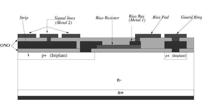
Figure 2: Diagram of the cross section of a PHOBOS silicon pad [81].

Voltage built up in the capacitor of a silicon pad was sent into a pre-amplifier and signal shaping chip that was bonded directly to the sensor. The chip was a 64-channel or 128-channel VA-HDR-1 chip, manufactured by the IDEAS company (http://www.ideas.no/). The pre-amplified signals were read out by Front-End Controllers, located in the experimental hall, that digitized the signals using 12 bit ADCs. These signals were then sent to the PHOBOS DAQ to be recorded (see Sect. 5).

3 Pedestal and Noise Correction

While the leakage current of the Silicon was minimized by the reverse-biased p-n junction, it was not zero. This current caused an offset to the signal read out from a Silicon channel, even if that signal would otherwise have been zero. The leakage current was roughly constant during one running of the silicon (during the time the reverse-biasing voltage was turned on), but could change by a small amount from one running to the next. Hardware offsets in the read-out system also contributed an overall offset to the Silicon signals. In addition, electronic noise in the system contributed an offset that would fluctuate from one event to the next.

The effect of these offsets could be measured by histogramming the signal from one Silicon channel over many events. In a typical collision event, it was unlikely that an ionizing particle had passed through any given silicon channel – in other words, the occupancy of the Silicon detectors was low. Thus, the lower part of the raw ADC distribution of a Silicon channel would provide a measure of the various offsets. This distribution was a Gaussian, the mean of which, known as the pedestal, reflected the overall offset due to electronic offsets and leakage current. The width of the Gaussian, referred to as the noise in the channel, was due to electronic noise and small fluctuations of the leakage current. Figure 3 shows the distribution of ADC values of a Silicon channel from many events, where the channel’s pedestal has been subtracted from the raw ADC signal in each event. The Gaussian pedestal/noise peak is clearly visible.

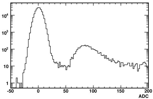
Figure 3: Pedestal-subtracted ADC distribution of a typical channel in the Ring detector. Note that the width of the Gaussian peak is roughly 5 ADCs channels.

The pedestal and noise were calculated in several steps. First, the raw ADC signals of each channel were averaged over 200 low multiplicity events. This pre-pedestal was then used to find a window in which to calculate the pedestal and noise. Next, ADC values within 100 ADC channels of the pre-pedestal from 600 low multiplicity events were histogrammed for each Silicon channel. The actual pedestal and noise were calculated in an even smaller window, found by locating the most populated bin of the histogram, and then stepping out in each direction until consecutive empty bins were encountered. Note that such bins are not seen in Fig. 3, since this figure shows the distribution from a large number of events, many of which had a high multiplicity. Finally, the peak in this small window was used to find the pedestal and noise. Silicon channels in the Octagon had the highest occupancy, and for those channels, the peak was fit with a Gaussian to extract the pedestal and noise values without contributions from actual deposited energy signals. For all other Silicon channels, the pedestal (mean) and noise ( Root-Mean-Square (RMS)) were calculated explicitly to save computing time. The pedestal and noise were then assumed to remain constant for about an hour of Silicon running time. Pedestal and noise values would be recalculated each time the Silicon bias was turned on and at least once an hour during Silicon data-taking.

After pedestal subtraction, the signal was further corrected for an offset effect known as Common-Mode Noise (CMN). This type of noise was the result of electronic cross-talk in the Silicon read-out chips. It caused an offset to the ADC which was different in each event, but in any given event the offset was the same for all channels being read out by the same chip. The amount of CMN was found by filling the pedestal-subtracted ADC of every channel in a given read-out chip into a histogram. This was done separately for every chip. The mean of this distribution, which would be close to zero in the absence of CMN, was taken to be the value of the CMN of that chip in the event. The mean was found by the same procedure used to find the pedestal: by calculating the mean in a small window about the most populated bin. However, the number of entries in the window was required to be above a certain threshold before a valid CMN correction could be performed. The CMN offset was then subtracted from the pedestal-subtracted ADC value. Typical values of the pedestal, noise and CMN-corrected noise are shown in Fig. 4. Notice that the CMN correction reduced the noise of the channels by roughly 20%.

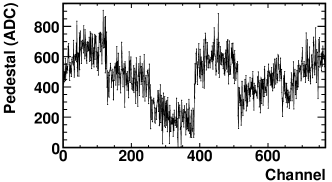
(a) Pedestal Values

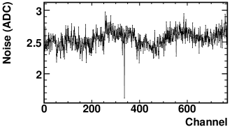
(b) Noise Values

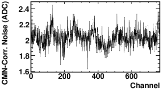
(c) CMN-Corrected Noise Values

Figure 4: Typical values of the pedestal and noise in Silicon channels. 4(a) Pedestal values. The 128-channel chips can be seen, as electronic offsets were implemented on a chip-by-chip basis. 4(b) Noise values (the width of the pedestal peak). 4(c) The noise of each channel after CMN-correction.

An additional CMN effect occurred in the Ring detectors. The capacitance of pads in the Ring detectors varied due to the changing pad size in the radial direction. This led to CMN that was not due to the read-out chip, but rather some Silicon effect, such as leakage current. The value of this CMN was found by assuming that all channels in a Ring sensor could have some constant offset and that the channels could have an offset that scaled with capacitance. Since the capacitance scaled with radial distance, the CMN offset was assumed to have two components: one that was a constant offset and one that varied linearly with radial distance.

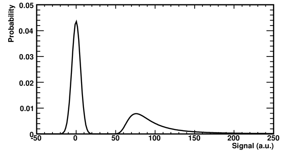
Figure 5: A typical model distribution (with no baseline shift) used in the maximum-likelihood fit to correct CMN in the Ring detectors.

The value of the baseline offset and slope were found on an event-by-event basis. The correction had to be done for every event, but occupancy in the Ring detectors could be very high in central collisions. This meant it was not possible to find the baseline using only information from channels with no signal from an ionizing particle. However, a baseline offset would shift the signal of channels at a particular radius by the same amount, whether the signal was due to a hit or not. This fact was exploited by the use of a maximum-likelihood fit. At each iteration of the fit, test values of the offset and slope were used to find a test baseline. This baseline was then used to shift a model signal distribution composed of a Gaussian pedestal and a Landau MIP peak, such as the one shown in Fig. 5. Eight model distributions were used, one for each radial position of pads in the Ring detectors. The likelihood that the signal of one channel came from the shifted model distribution was taken as the height of the distribution at the location of the signal. Thus, the most likely baseline would shift the model distributions such that most of the signals of all channels in a Ring sensor were under a peak – either the pedestal peak or the MIP signal peak. Once the best baseline offset and slope parameters were obtained, the baseline was calculated for each radial position and subtracted from the signal in each channel of the Ring detectors.

4 Energy Calibration

Once the offset of the signal in a Silicon channel had been corrected, it was possible to extract the amount of energy deposited into a pad using the ADC signal in the channel. For this to be possible, it was necessary to measure the factor by which the shaper and pre-amplifier chips amplified the signal created by charge collected in a Silicon pad. This factor is known as the gain of the chip, but the term ‘gain’ is also commonly used by physicists to refer to the ratio between deposited energy and ADC value.

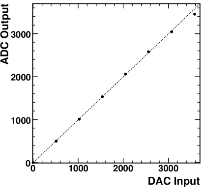
Figure 6: The ADC output signals of a typical Silicon read-out chip generated by eight different DAC input signals. The slope of the line (1.00) is the gain of the chip.

Calibration circuitry was built-in to each read-out chip to allow the electronic gain of the chip to be measured. This was done by sending known Digital-to-Analog Converter (DAC) signals into the chip and measuring the output ADC signals. Special calibration runs were taken by the experiment to measure the gains of all Silicon read-out chips. In these runs, eight different DAC signals were used to measure the gain of the chip as a function of input signal. As shown in Fig. 6, the relationship between input DAC and output ADC was linear over almost the entire dynamic range of the read-out chips (the 12 bit ADC had values ranging from 0 to $2^{12}-1=4095$). The slope of this line was the gain of the read-out chip. Typically, the gain of a chip was very close to one.

The gain of the chip related the digital output ADC value to the digital input DAC value, but more information was required to use this gain to extract the amount of deposited energy from a measured ADC value. The input DAC signal was generated by charging a capacitor, with capacitance $C_{t}$, such that it stored enough charge to produce a signal of $V_{c}$ volts per DAC. Typical values for $C_{t}$ were around $2.14~{}\mbox{${\rm pF}$}$, while the calibration electronics typically produced a signal with $V_{c}\approx 4.33\times 10^{-2}~{}\mbox{${\rm mV}$}/\rm\acs{DAC}$. These parameters, combined with the gain of each chip, were sufficient to relate an output ADC value to the amount of charge that created the signal sent into the chip. Of course, this relation was the same for charge produced by the calibration circuitry as it was for charge created by an ionizing particle. At room temperature, the average energy required to create an electron-hole pair in silicon is 3.62 ${\rm eV}$ (it increases as the temperature is decreased, to 3.72 ${\rm eV}$ at 77 Kelvin [82]). Combining this with the charge of an electron, $1.6022\times 10^{-4}~{}\mbox{${\rm fC}$}$, it was possible to relate the output ADC signal, $A_{s}$, to the amount of energy deposited into the Silicon pad

$$E_{dep}(A_{s}) =\frac{A_{s}}{\rm gain}\>V_{c}\>C_{t}\>\frac{3.62\mbox{${\rm eV}$}/e}{1.6022\times 10^{-4}\mbox{${\rm fC}$}/e}$$ (2)

$$\approx\frac{A_{s}}{1\rm\acs{ADC}/\rm\acs{DAC}}\left(0.0433~{}\frac{\mbox{${\rm mV}$}}{\rm\acs{DAC}}\right)(2.14~{}\mbox{${\rm pF}$})\left(22.6~{}\frac{\mbox{${\rm keV}$}}{\mbox{${\rm fC}$}}\right)$$

$$\approx A_{s}\times 2.09\mbox{${\rm keV}$}/\rm\acs{ADC}$$

5 Event-by-event Energy Correction

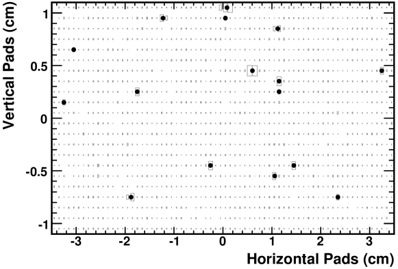
Figure 7: An example of merged hits in a Spectrometer sensor. The size of the grey boxes shows the amount of energy deposited in each pad of the sensor. The black circles show the resulting merged hit locations.

With the amount of energy deposited into each Silicon pad known, it was possible to improve the estimation of where the particle traversed the detector. Electron-hole pairs could be collected in multiple pads if an ionizing particle passed through the detector near the edge of a pad or at an angle that was not normal to the detector. These situations were taken into account by attempting to merge several adjacent hits. For Spectrometer channels, hit merging was performed in the horizontal direction. For most Spectrometer silicon sensors (the only exception being Type 1 sensors), pad sizes were much smaller in the horizontal direction than in the vertical and it was not unreasonable to expect that adjacent hits in the vertical direction were due to more than one particle. Adjacent Spectrometer channels that had recorded more than 15% of the energy a MIP would deposit were used to find the merged hit. The locations of up to eight such adjacent hits were averaged, each weighted by the energy of the hit. The averaged position was taken as the location of the hit, and the sum of the deposited energy of the individual hits was taken as the energy of the merged hit. Merged hits were required to have a total deposited energy greater than half of a MIP. An example of merged hits on a Spectrometer sensor is shown in Fig. 7.

2 Zero-Degree Calorimeter Energy Calibration

The PHOBOS ZDC detectors were used to measure the total energy of particles. Raw signals measured by the detectors were corrected for an overall offset and a calibration scale-factor.

1 Čerenkov Detectors

Some materials have refractive properties that slow the progression of light through the material. While light is slowed in the material, a fast moving charged particle will not be. Thus it is possible for a charged particle to pass through the material at speeds greater than the speed at which light can travel through the material. When this happens, an electromagnetic shock wave occurs. This shock wave is known as Čerenkov radiation. The goal of the PHOBOS ZDC detectors was to stop neutrons and measure the Čerenkov radiation generated by charged particles in the resulting particle shower. The total Čerenkov radiation collected could then be related to the energy of the original neutron.

In an infinite radiating medium, all Čerenkov radiation is emitted in a single coherent wave front, shaped like a cone. For this ideal case, the Čerenkov light is emitted at a single angle relative to the charged particle’s trajectory. In a finite medium, there is a set of discrete angles at which light is emitted. Nevertheless, the majority of light is emitted at the same angle as for the ideal case, so it is of interest to determine this angle. Because the index of refraction of the radiating material, $n$, is known, it is not difficult to calculate the angle at which light is emitted from the Čerenkov cone to be $\theta_{C}=\arccos\left(\frac{c}{vn}\right)$, where $v$ is the speed of the charged particle and $c$ is the speed of light in a vacuum [83]. Thus, the speed of the particle must be greater than the speed of light in the material ($c/n$), or the angle is undefined and no Čerenkov radiation occurs.

Čerenkov detectors are commonly built to exploit the dependence of the emission angle on particle velocity and index of refraction in two ways. First, the index of refraction of the radiating medium can be changed to alter the minimum kinetic energy a particle of a certain type must have in order to be observed. This is commonly done by using a liquid or gas whose index of refraction can be changed by varying its pressure. Such an energy threshold can be used to reject particles from a measurement that would otherwise contribute to the measurement’s background. Second, the speed of the particle can be identified by measuring the angle of the Čerenkov cone. This can be used to determine the type of particle being observed. Note that neither of these techniques were used by the PHOBOS ZDCs.

2 Photomultipliers

Light generated from Čerenkov radiation is collected and converted to an electric signal by Photomultiplier Tubes (PMTs). Photomultipliers generally consist of several different components: a photocathode that converts photons to electrons, an electron input system that collects the photo-electrons, a dynode string that creates an electron cascade and finally an anode from which the electronic signal can be read out [84].

The photocathode produces electrons via the photoelectric effect. This quantum mechanical effect is described by the well known function, the discovery of which won Einstein his Nobel prize, $E=h\nu-\phi$, where $E$ is the energy of the emitted electron, $\nu$ is the frequency of the incident photon and $\phi$ is the work function of the emitting material. Thus there is a minimum frequency of light that can produce a photoelectron in a given material. However, even for photons having a frequency above this threshold, it is not certain that an electron will be emitted and the probability of producing a photoelectron in a given material can depend strongly on the frequency of the photon. For physics experiments, photocathode materials are chosen such that the efficiency of producing photoelectrons, known as the quantum efficiency, is peaked for the photon wavelengths produced by the Čerenkov or scintillator detector being constructed. Typically, such light is in the visible range, having wavelengths around 400 ${\rm nm}$ (which appears blue).

The photoelectrons are then collected and directed to the multiplier section. Collection in the electron input system is typically achieved by an electric field that directs electrons onto the first dynode of the multiplier section. A well designed electron input system can collect all electrons from the photocathode, independent of the position from which they were produced on the photocathode. That is, the electron input system should collect all electrons with the same efficiency and direct all electrons from the cathode to the dynode string in the same amount of time.

The dynode string amplifies the photoelectron current by using a series of secondary emission electrodes, known as dynodes (hence the name). At the first dynode, the photoelectrons strike the electrode and release secondary electrons from the dynode material. The secondary electrons are then accelerated through a static electric field to the next electrode. This process is repeated at each step of the dynode string, resulting in an electron cascade. A well designed electron multiplier uses dynode material that has a high secondary electron emission factor yet does not emit electrons due to thermal energy (which would result in noise). It is also important that the dynode material can emit secondary electrons in a stable manner when placed under high currents. After being amplified by the electron multiplier, the photoelectron current is collected at the anode and passed out of the PMT as an electric signal to be recorded by a DAQ system.

3 Pedestal and Noise Correction

As with all detectors, the ZDC signals had to be corrected for various offsets. The pedestal was mainly due to electronic offsets in the readout system and leakage currents in the phototubes. Offsets that fluctuated from one event to the next included electronic noise as well as statistical and thermal fluctuations in secondary electron emission within the PMTs. Thermal emission of electrons by the photocathode and dynodes resulted in an electric current that was independent of any light being incident on the PMT. Statistical fluctuations, on the other hand, originated from the inherit randomness associated with the photoelectron and secondary electron emission processes.

The pedestal and noise of ZDC channels was measured by observing the ADC signal distribution of each channel from a collection of events in which no signal was expected to be present. Such events could be identified by checking that the channel’s TDC produced no signal or by requiring that the RHIC accelerator was not colliding particles during that particular bunch crossing. The resulting ADC distribution was then fit with a Gaussian, from which the mean and width were taken to be measures of the pedestal and noise in the channel.

4 Energy Calibration

The ZDC detectors had the great advantage that the majority of particles it was built to observe had a known energy. Most free spectator neutrons had an energy equal, or very close, to 100 ${\rm GeV}$. This fact was exploited to calibrate the ZDC ADC signal. A ZDC module could detect one, two or, with decreasing probability, some larger number of neutrons. Because each neutron deposited roughly the same amount of energy, neutron peaks were expected (and observed) in the ADC distribution of a ZDC channel from many collisions. The first peak could then be assumed to correspond to an incident energy of 100 ${\rm GeV}$, the second to 200 ${\rm GeV}$ and so on.

The energy calibration of each ZDC detector, i.e. the Au-side and d-side, was done separately and in several steps. First, the pedestal-subtracted ADC distribution of a particular ZDC channel was plotted for collision events in which the channel reported a signal above the pedestal, while the other two channels of the detector did not. The resulting one-neutron peak of this distribution was then fit with a Gaussian. The mean of the Gaussian divided by 100 ${\rm GeV}$ gave an estimate of the energy calibration factor for the channel. This method yielded calibration factors for the three channels of a ZDC detector that agreed to within about 20%.

The calibration of a ZDC detector was then improved by varying the calibration factors of individual channels such that the best possible energy resolution was achieved. First, the calibration factor of the ZDC module nearest the IP was held constant, while the calibration of the middle module was varied over $\pm 50\%$. The sum of the signals in the two channels was then plotted for each step. Each resulting one-neutron peaks was fit with a Gaussian. The best relative calibration factor between the front two modules, $f_{1}$, was taken to be that which minimized the width of the resulting peak. This process was then repeated by holding $f_{1}$ constant and varying the relative calibration of the module furthest from the IP. At each step, the sum of the signals from all channels was then plotted and fit with a Gaussian. The best relative calibration factor between the back module and the other two modules, $f_{2}$, was taken to be that which minimized the width of the resulting peak. For events in which all three modules of the deuteron-side ZDC showed a signal above the pedestal, this method yielded an energy resolution of $\sigma/E\approx 30\%$ for that detector ($\sigma$ being the width of the one-neutron peak).

3 Proton Calorimeter Energy Calibration

Like the ZDCs, the PCAL detectors were also used to measure the total energy of particles. Raw signals measured by the detectors were corrected for an overall offset and a calibration scale-factor.

1 Scintillator Detectors

Particles passing through scintillator material collide with the atoms and molecules in the material. The excited atoms and molecules decay to their ground state by radiating the extra energy in the form of photons. The detector measures the number of photons produced, and from this information the amount of energy deposited into the detector can be determined.

Scintillator detectors are used both for their fast time response and for the linear proportionality of light output with deposited energy. A good scintillator material for particle detection is one that (a) efficiently radiates excitation energy as fluorescent light, (b) is transparent to the fluorescent light, (c) emits fluorescent light at wavelengths that can be efficiently detected (by PMTs) and (d) quickly returns to its ground state after being excited.

The time evolution of light output from a scintillator material can be expressed by a two-component exponential

$$N=A\exp\left(\frac{-t}{\tau_{f}}\right)+B\exp\left(\frac{-t}{\tau_{s}}\right)$$ (3)

where $\tau_{f}$ and $\tau_{s}$ are the fast and slow time-decay constants, respectively. Note that while the rise time of light output is finite, it is typically so much faster than the decay time that it has been taken to be zero in Eq. 3. For some materials, the prompt and delayed components of the decay time can depend significantly on the type of particle that excites the scintillator. In such cases, it is possible to identify the type of particle by examining the resulting pulse shape (this technique was not employed for the PHOBOS PCALs). The scintillating material used in the PCAL detectors had a prompt decay time of 3.2 ${\rm ns}$ and no significant delayed component. Light emitted by scintillator material is detected using photomultiplier tubes (see Sect. 2).

2 Pedestal and Noise Correction

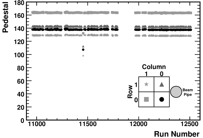
Figure 8: The pedestal values for each channel in the d-PCAL versus the PHOBOS DAQ run number, which is increasing with time. The large gap separates the d+Au physics run (lower numbers) from the p+p physics run (higher numbers). Also shown is the row and column numbering convention for PCAL detectors.

The main sources of signal offsets in the PCAL detectors were similar to those of the ZDCs; namely electronic offsets in the readout system and various PMT effects. The pedestal and noise were determined by examining the ADC distribution of each channel over at least six hundred heartbeat events. Heartbeat events were not triggered by any physical collision property, but rather were periodic readouts of the entire detector system by the PHOBOS DAQ. Thus, it was very improbable that any physical particle had deposited energy into a PCAL channel during the 100 ${\rm ns}$ window in which the detector’s signals were recorded. The mean and RMS of each distribution was then directly calculated and taken to be the channel’s pedestal and noise, respectively. The pedestals of the PCAL channels were found to be quite stable over time, as shown in Fig. 8.

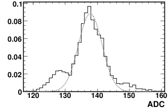
(a) A Pedestal Distribution

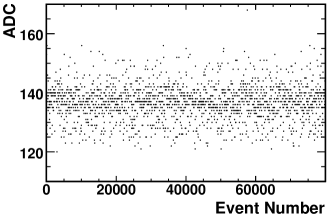
(b) ADC vs Time

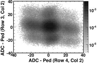
(c) Channel Correlation

Figure 9: Structure in the pedestal PCAL ADC distribution. 9(a) The ADC distribution of signals in a PCAL channel from heartbeat events. A Gaussian fit to the central peak is shown by the grey, dashed line to guide the eye. Note the secondary peak at the low end of the pedestal and the non-Gaussian tail at the high end. 9(b) Signals of a PCAL channel from heartbeat events versus time. No baseline drift is observed. 9(c) Pedestal-subtracted ADC signals from heartbeat events of one PCAL channel versus an adjacent channel. No correlation is present that would suggest a CMN effect.

While the pedestals were stable with time in the PCAL detectors, the shape of the pedestal peak was not simply a Gaussian, as would be expected given a stable, constant offset and some random noise. In addition to a central peak, some PCAL channels exhibited large tails and/or smaller, displaced peaks. An example is shown in Fig. 9(a). While an offset that shifts or jumps with time in a systematic, rather than random, way could explain such an ADC distribution, such behavior was not seen. Figure 9(b) shows that the ADC signals reported by a single PCAL channel were not correlated with time in a systematic way. In addition, it was found that the effect was due to the detector, most likely the PMTs, and not the readout system, as the ADC distributions were not changed by connecting the detector to an alternate readout system. Finally, it was thought that the effect may be due to common-mode noise. However, no correlation of signals between channels was observed in heartbeat events, as shown in Fig. 9(c). Thus, since the effect could not be corrected for, it was intentionally taken into account by estimating the pedestal and noise from a direct calculation of the mean and RMS of the full distribution, rather than from a Gaussian fit to the central peak.

3 Energy Calibration

Au-PCAL Calibration

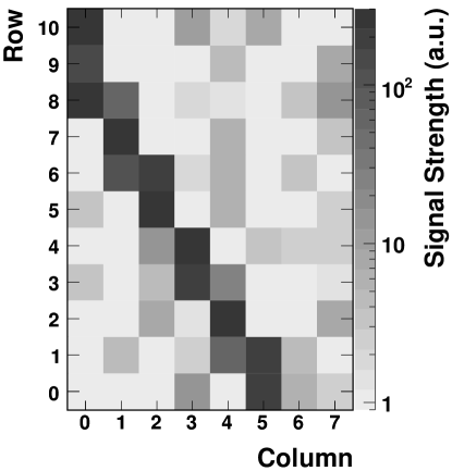
Figure 10: A display of the energy deposited into the Au-PCAL by a cosmic ray. Modules are represented by squares; the dark grey diagonal “line” shows the path of the cosmic ray. Light grey squares simply show noise in the Au-PCAL read-out and detector electronics.

The energy deposited into the Au-PCAL was determined by using cosmic rays to calibrate the detector. This was necessary because the Au-PCAL, unlike the ZDC and the d-PCAL, did not observe a single-hadron peak in the d+Au data. A sample display of a cosmic ray detected by the Au-PCAL is presented in Fig. 10. To calibrate the detector with cosmic rays, it was necessary to estimate the amount of energy that cosmic ray muons were expected to deposit in a PCAL module. This was done using the Bethe-Bloch formula (see Eq. 1) and assuming that, on average, a cosmic muon traveled about 10.8 ${\rm cm}$ through a $10\times 10~{}\mbox{${\rm cm}$}$ calorimeter block, of which 1.9 ${\rm cm}$ was through scintillator material and 8.9 ${\rm cm}$ was through lead. From this, it was estimated that only muons having roughly 1.5 ${\rm GeV}$ kinetic energy were able to traverse the entire calorimeter and deposit energy into cosmic ray trigger modules both above and below the Au-PCAL. The average kinetic energy of muons incident on the calorimeter was expected to be around 4 ${\rm GeV}$. Finally, it was estimated that on average, cosmic ray muons would deposit around 145 ${\rm MeV}$ of energy into a PCAL module (lead and scintillator combined).

This information was used to calibrate the detector by assuming that 145 ${\rm MeV}$ of energy deposited by a muon should produce the same amount of scintillator light as 145 ${\rm MeV}$ of energy deposited by a proton (Eq. 6). However, the calibration was further complicated by the fact that the voltages used to power the calorimeter’s PMTs during cosmic ray data taking were different from those used to take d+Au physics data. The differing voltages were required since spectator protons from a high-energy d+Au collision were expected to deposit much more energy than a cosmic ray muon. Thus, it was necessary to measure how the overall amplification of the PMTs changed with voltage. This was done for a collection of tubes using a Light-Emitting Diode (LED) as a light source, and it was found that the gain of the tubes was described by

$$A=kV^{8.93}$$ (4)

where $A$ is the signal reported by the tube, $V$ is the voltage and $k$ is some constant of proportionality.

The energy deposited by a cosmic ray muon was

$$E_{C}=G_{C}A_{C}$$ (5)

where $E_{C}$ is the energy deposited by the muon, $G_{C}$ is the energy calibration factor at the cosmic ray voltage and $A_{C}$ is the signal generated by the muon. From Eq. 4, it was then possible to find the energy calibration factor for d+Au collisions, $G_{D}$, to be

$$E_{D} =E_{C}$$ (6)

$$G_{D}A_{D} =G_{C}A_{C}$$

$$G_{D}kV_{D}^{8.93} =G_{C}kV_{C}^{8.93}$$

$$G_{D} =G_{C}\left(\frac{V_{C}}{V_{D}}\right)^{8.93}$$ (7)

The value of $G_{C}$ was calculated given that $E_{C}=145~{}\mbox{${\rm MeV}$}$ for the average cosmic ray muon and that the signal reported by such a muon was just the mean of the muon-peak in the cosmic ray data, $A_{CP}$. Thus the energy deposited by a proton from a d+Au collision, $E_{D}$, as a function of the signal reported by a module, $A_{D}$, was

$$E_{D}(A_{D}) =G_{D}A_{D}$$

$$=G_{C}\left(\frac{V_{C}}{V_{D}}\right)^{8.93}A_{D}$$

$$=\frac{145~{}\mbox{${\rm MeV}$}}{A_{CP}}\left(\frac{V_{C}}{V_{D}}\right)^{8.93}A_{D}$$

$$E_{D}(A_{D}) =145~{}\mbox{${\rm MeV}$}\frac{A_{D}}{A_{CP}}\left(\frac{V_{C}}{V_{D}}\right)^{8.93}$$ (8)

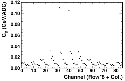
Figure 11: Values of $G_{D}$ used during d+Au physics running for channels in the Au-PCAL.

Typical values of $V_{C}$ were $\sim 1450~{}\mbox{${\rm V}$}$, while typical values of $V_{D}$ were $\sim 1150~{}\mbox{${\rm V}$}$. The values of $G_{D}$ used to process the d+Au data are presented in Fig. 11. The spread in gain values is a result of the variation of $V_{D}$ from module to module. Voltages used during d+Au physics running were adjusted for each module such that a majority of the dynamic range of ADC signals was used. Note in particular the two channels with very large gain. These channels were nearest the beam pipe, in column zero, rows four and five (see Fig. 10). Much more energy was deposited into these two channels during d+Au physics running than into any of the other channels. To compensate for this, filters were installed into the PMTs of these two channels that absorbed 80% of the scintillator light. This allowed these PMTs to be operated at voltages that were closer to, but still somewhat lower than, the voltages of PMTs on other channels. This lower voltage was the cause of the large gain values for these two modules.

PCAL Simulations

Figure 12: Signal distribution of two Au-PCAL modules in the d+Au data. See Fig. 10 for a diagram of the module positions; the beam line was closest to modules (4,0) and (5,0), located between rows 4 and 5 in the vertical direction.

After energy calibration, it was found that the distribution of signals from modules closest to the beam line, those in column zero, exhibited a different shape compared to those of other modules, as shown in Fig. 12. The modules nearest the beam line showed a peak in the signal distribution. To investigate the origin of this excess signal, simulations of the calorimeters were performed. First, an extensive accounting of the RHIC accelerator material, including the DX-magnet structure and beam pipes, was obtained to ensure that the simulation geometry was accurate. Then, four types of nucleons were simulated, (a) uninteracted deuteron nucleons, (b) elastically scattered deuteron nucleons, (c) thermally radiated gold nucleons and (d) gold nucleons emitted from a nuclear fragmentation cascade.

All four types were simulated using very simple models. The uninteracted deuteron nucleons were simulated using the beam momentum, including the $\sim 1~{}\mbox{${\rm mrad}$}$ angular offset of the beam and the spread in initial vertex positions due to the width of the beam. Taken from measurements of the spread of d+Au interaction vertices, the beam was described as having a Gaussian shape in the transverse directions, with an RMS of 0.122 ${\rm cm}$ in the horizontal and 0.097 ${\rm cm}$ in the vertical direction. The elastically scattered deuteron nucleons were simulated by randomly sampling the transverse momentum from the relation

$$\frac{1}{p_{\mathrm{T}}}\frac{d\!N}{d\!p_{\mathrm{T}}}=\exp\left(\frac{-p_{\mathrm{T}}^{2}}{T_{e}}\right)$$ (9)

where $T_{e}\sim 100~{}\mbox{${\rm MeV}$}$, a parametrization inspired by previous studies, see for example [85]. The longitudinal momentum was then calculated such that the total momentum of the nucleon was equal to the beam momentum. The beam angle and width were then added to the initial origin and momentum of the nucleon. The gold nucleons were simulated by randomly choosing the kinetic energy of the nucleon in the gold nucleus rest frame by sampling the relation

$$\frac{d\!N}{d\!E}=\sqrt{E-B}\exp\left(\frac{-(E-B)}{T}\right)$$ (10)

where $B\sim 10~{}\mbox{${\rm MeV}$}$ represents a Coulomb barrier [86] and $T$ was taken to be 50 ${\rm MeV}$ for the cascade nucleons [86] and 8 ${\rm MeV}$ for the thermal nucleons [87]. The angular orientation of the nucleons in the gold nucleus rest frame was then chosen randomly, according to the angular distributions given in [88]

$$\frac{d\!N}{d\!\cos\theta}\propto\left(\frac{4}{\sqrt{\pi}}\chi_{0}\cos\theta\right)$$ (11)

where $\chi_{0}$ is a parameter related to the velocity of the fragmenting nucleus and the nucleon. Its value is taken to be 0.45 for cascade nucleons and 0.11 for thermal nucleons (see [88]). The nucleons were then boosted by the beam rapidity into the lab frame.

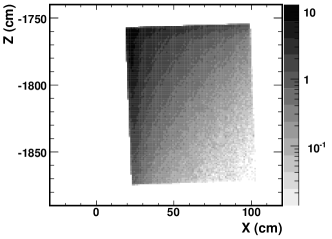
(a) Z-X Distribution

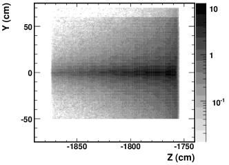
(b) Y-Z Distribution

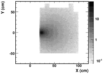
(c) Y-X Distribution

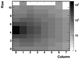
(d) Modules

Figure 13: Energy deposited into the Au-PCAL by thermally radiated nucleons in simulations.

The nucleons were then swum from the IP and through the magnetic field of the DX-magnet using the Geant simulation package [89]. Both protons and neutrons were simulated for each possible type of signal nucleon. An example that shows the location and amount of energy deposited into the Au-PCAL by thermally radiated nucleons is shown in Fig. 13. It can be seen that the majority of the energy from the nucleons was deposited into the two modules nearest the beam line.

These simulations revealed that protons traversed a significant amount of magnet iron as they passed through the DX-magnet, causing the protons to lose energy prior to entering the calorimeter. Thus it was expected that this detector would have a lower efficiency than the ZDC; see Sect. 3. However, they showed that the signal from such protons was not blocked completely, and the distribution of energy deposited into the PCALs in the simulations was found to agree reasonably well with the data. Further, these simulations suggested that a substantial fraction of the excess signal seen in the Au-PCAL column nearest to the beam line was due to neutron shower leakage from the ZDC. Attempts to correct for this effect by subtracting from the Au-PCAL signal an amount of energy proportional to the signal seen in the Zero-Degree Calorimeter on the Au-exit side (Au-ZDC) did not improve the energy resolution. It was assumed that fluctuations in the calorimeter signals were too large for this procedure to work. In the end, only energy deposited into modules from rows four and five, as well as modules in columns four through seven, was included in the definition of the Energy in Au-PCAL (EPCAL) variable (see Sect. 3). Signals measured by all modules in rows four and five were included in this variable because the energy deposited by spectator protons was expected to be much larger than any deposited energy due to shower leakage from the ZDC, as seen in Fig. 13(d). Such an assumption was not made for the signals reported by modules near the beam line in other rows.

While the signal measured by the d-PCAL should have been influenced by the Zero-Degree Calorimeter on the d-exit side (d-ZDC) in a similar manner, it was not a significant effect due to the smaller amount of energy that was deposited into the d-PCAL during a d+Au collision. As can be seen in Fig. 17 on page 17, the effect did not contaminate the set of nucleon-nucleus tagged data; see Sect. 2.

d-PCAL Calibration

Modules in the d-PCAL were calibrated to be consistent relative to each other, but not to any absolute energy scale. A relative calibration of the d-PCAL modules was sufficient since this detector was only used to discriminate between collision types, not to measure the energy of the signal. Since the distribution of signals over many events from channels in the d-PCAL contained a peak, it was possible to calibrate the detector using a method similar to that used for the ZDCs. The modules were calibrated relative to each other in several steps. First, the channel at $(\text{row,column})=(0,0)$ (see Fig. 8 for the numbering convention) was chosen as the reference channel. Next, vertically adjacent channels were gain-matched relative to each other. This was done by varying the relative gain, $G_{0}$, between channels (0,0) and (1,0) and plotting the sum $A_{0,0}+G_{0}A_{1,0}$, where $A_{1,0}$ is the signal in channel (1,0), over many events. The relative gain factor that minimized the width of the peak in the resulting distribution was then taken to be the best estimate of the relative calibration. The same process was performed for the column further from the beam pipe, to find the best relative gain factor $G_{1}$. Finally, the two columns of the detector were calibrated relative to each other. This was done by varying the relative gain, $G_{C}$, between column 0 and column 1 and plotting the sum $A_{0,0}+G_{0}A_{1,0}+G_{C}(A_{0,1}+G_{1}A_{1,1})$. Examples of this are shown in Fig. 14(a). The relative gain factor that minimized the width of the peak in the resulting distribution was taken to be the best estimate of the relative gain factor between the two columns, as shown in Fig. 14(b).

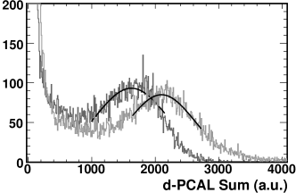
(a) Varying Relative Gain

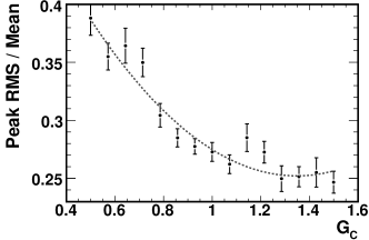
(b) Minimizing Peak Width

Figure 14: Steps used to find the relative calibration factors for d-PCAL channels. 14(a) Example distributions of the full d-PCAL signal using two different relative gain factors between the columns. The black lines show Gaussian fits to the peaks. 14(b) The width of the peak, as measured by the RMS/mean of the Gaussian fit, versus relative gain factor. The dashed grey line shows a parabolic fit. The minimum of the fit was taken to be the best estimate of the relative calibration.

Chapter 3 Collision Reconstruction

After the amount of energy deposited into each detector channel had been determined, it was possible to deduce various physical properties of the collision. Information about the location, magnitude and, in some cases, time of each hit in the PHOBOS detector was used to ascertain the collision’s usefulness for physics analysis, its geometry and its location.

1 Collision Triggering

During the d+Au physics run, PHOBOS made use of several different algorithms to determine when a desirable collision had occurred. Each of the algorithms imposed certain criteria on the responses of the fastest detectors to trigger the read-out of the entire experiment. Three different trigger types were used by the analysis presented in this thesis: dAuMinBias, dAuVertex and dAuPeriph.

1 The dAuMinBias Trigger

The d+Au Minimum Bias (dAuMinBias) trigger was used to build a statistical sample set of events that most accurately represented the full d+Au collision population. The bias in the sample set was minimized by placing loose restrictions on the number of particles produced as well as the regions of phase space filled by produced particles. This was done using the Paddle detectors (see Sect. 4), which had a large geometrical acceptance.

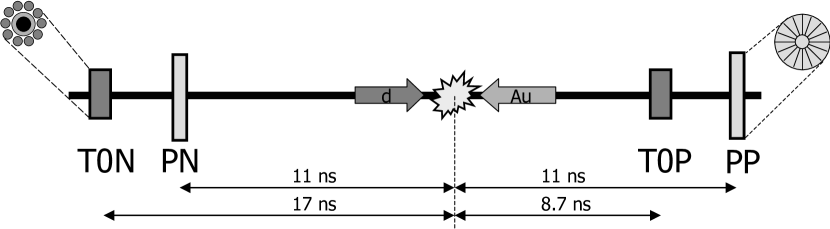
Figure 1: The location of trigger detectors during the d+Au physics run. Distances are shown by the amount of time it took light to travel from the IP to each detector. ‘T0N’ and ‘T0P’ refer to the Au-side and d-side T0s, respectively, while ‘PN’ and ‘PP’ refer to the Paddle detectors [90].

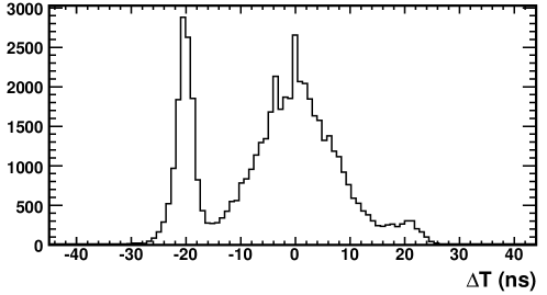
Figure 2: The paddle time difference distribution from roughly 54k dAuMinBias triggered events. The peaks at $\pm 22~{}\mbox{${\rm ns}$}$ can be attributed to beam-gas collisions.

The dAuMinBias trigger required that at least one channel in each Paddle detector report a hit during a specified time window. This provided the first clue that some sort of collision had taken place. An even more unbiased trigger could be imagined, in which only a single Paddle channel needs to be hit. However, a single-arm trigger would fire on many events that would be unusable for analysis, such as collisions between the beam and gas inside the beam pipe. Such beam-gas collisions can, of course, occur at any position along the beam direction. The dAuMinBias trigger reduced the number of beam-gas events measured by the experiment by requiring that the two Paddle hits occurred within 38 ${\rm ns}$ of each other. As shown in Fig. 1 [90], the Paddles were only 22 ${\rm ns}$ apart. Thus, the largest time difference between hits in the two Paddles caused by particles produced in the same collision would be 22 ${\rm ns}$ plus some measurement error in the timing. Therefore, the large timing window of 38 ${\rm ns}$ served to select all collisions that produced hits in both Paddles. This loose requirement was necessary to construct a minimally biased collision sample, but it also allowed many beam-gas collisions to be triggered, as shown in Fig. 2.

2 The dAuVertex Trigger

The d+Au Vertex (dAuVertex) trigger was used to record collisions that were more likely to produce particles in the Spectrometer acceptance. This was achieved by selecting collisions that occurred within 50 ${\rm cm}$ of the IP. A timing coincidence between the T0 detectors was used to enforce this vertex requirement. The T0s had a much better timing resolution than the Paddles (roughly an order of magnitude better), resulting in a more precise vertex resolution, but they had a smaller acceptance than the Paddles. This smaller acceptance introduced a non-negligible centrality bias in the dAuVertex trigger. Central d+Au collisions yielded more particles than peripheral collisions, making them more likely to produce a hit in each of the T0 detectors. Thus, for a central and a peripheral collision both occurring exactly at the IP, the peripheral collision would be less likely to produce particles which hit the T0s and thereby fire the dAuVertex trigger. To facilitate a study of this centrality bias, when the PHOBOS experiment would take data, it would not use the dAuVertex trigger exclusively. Instead, when taking primarily dAuVertex triggered data, a small fraction of the data recorded by the experiment would be dAuMinBias triggered collisions.

3 The dAuPeriph Trigger

The d+Au Peripheral (dAuPeriph) trigger was used to specifically select collisions with large impact parameters. The goal of this trigger was to build a set of data that complemented the centrality-biased dAuVertex triggered data by being biased toward peripheral collisions. This was achieved by first keeping the vertex requirement from the dAuVertex trigger and then adding a further requirement that no more than eight channels in the Au-side Paddle detector be hit. The low-multiplicity requirement served to reduce the amount of central collision data taken, thereby increasing the relative number of peripheral collisions in the data. As done for the dAuVertex triggered data, a small fraction of the data recorded while running primarily with the d+Au Peripheral (dAuPeriph) trigger consisted of dAuMinBias triggered collisions.

2 Vertex Reconstruction

While the Paddle and T0 detectors were used to quickly estimate the position of a collision during data-taking, a more precise measurement was obtained offline, using silicon detectors. In Au+Au collisions, the large number of particles released allowed the collision location to be determined by simply finding a common origin of tracks in the Spectrometer and Vertex detectors. The relatively low multiplicity produced by d+Au collisions, on the other hand, made it necessary for a different measurement technique to be adopted. The location of a collision along the beam axis (the $z$ direction) was obtained using the Octagon. The transverse vertex position was determined using the Spectrometer and the Vertex detectors.

Since the Octagon had only a single layer of silicon, no particle tracks could be reconstructed using the detector. However, the amount of energy deposited into an Octagon pad could, in fact, be used to gain information about how a particle might have traversed the silicon. Large energy depositions were generally due either to a slow particle (see Fig. 1) or a particle which passed through the silicon at a shallow angle. Most slow particles were produced not by the d+Au collision itself, but rather by a secondary collision in which a product of the d+Au collision interacted with some material. Such secondaries would not necessarily be produced anywhere near the original collision. Therefore, a hit due to a secondary particle would always have a large energy deposition, even after attempting to correct for the increased path length of a particle coming from the collision vertex.

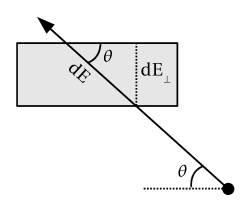
Figure 3: Correcting the deposited energy ($\mathit{dE}$) for the incident angle ($\theta$) of a particle coming from the vertex.

The Octagon Deposited Energy (OctDe) vertexing algorithm assumed that each Octagon hit was due to a primary particle passing through the silicon at an oblique angle. First, the energy from three adjacent pads along the beam direction was combined. The angle of the resulting merged hit was determined by the collision position and center of the first merged silicon pad (furthest along the beam line toward the Au-side). Note that the weighted average method described in Sect. 5 was not used to find the merged hit position. Then for some chosen test vertex, the deposited energy of each Octagon hit was corrected for the path length of particles through the silicon, as shown in Fig. 3,

$$\mathit{dE}_{\perp}=\mathit{dE}\sin(\theta)=\frac{\mathit{dE}}{\cosh{\eta}}$$ (1)

$${}\eta=-\ln\left(\tan\frac{\theta}{2}\right)$$

where $\mathit{dE}$ is the total deposited energy of the hit, $\theta$ is the angle of the particle coming from the collision vertex, $\mathit{dE}_{\perp}$ is the amount of energy a perpendicularly incident particle would deposit and $\eta$ is the pseudorapidity of the particle. The best estimate of the vertex was then taken as the one which resulted in the fewest hits due to secondaries – or equivalently, the largest number of MIPs. After the deposited energy was angle-corrected, any hit that had between 70 ${\rm keV}$ and 110 ${\rm keV}$ of deposited energy was identified as being due to a MIP. The longitudinal vertex position resolution of the OctDe algorithm ranged from 0.7 ${\rm cm}$ for central collisions to 1.3 ${\rm cm}$ for peripheral collisions [91].

(a) Horizontal Beam Orbit

(b) Vertical Beam Orbit

Figure 4: The beam orbit as a function of time during the d+Au collision data taking. 4(a) The average horizontal, $x$, position of the beam. 4(b) The average vertical, $y$, position of the beam.

Tracks in the Spectrometer and Vertex detectors were used to determine the average transverse position of collisions. Due to the low number of tracks produced in a d+Au interaction, it was not possible to measure the transverse position of each individual collision. However, since the RHIC beams were tightly bunched in the transverse plane, the position of a collision was determined primarily by the position of the beams. This allowed the average horizontal, $x$, and vertical, $y$, positions of the beam orbit to be determined for a given set of collisions [37]. The origin of straight tracks in the magnetic field-free region of the Spectrometer and of tracks in the highly segmented Vertex detector were determined for each event by finding the average intersection point of the tracks in the event. The average (over several collision events) of the $x$ and $y$ positions of these track origins were taken to be the beam orbit for that collection of collisions. The beam orbit showed a relatively small spread in transverse vertex position (0.4 ${\rm mm}$) compared to the resolution obtained by simply using the origin of single tracks [91]. The beam orbit $x$ and $y$ positions are shown in Fig. 4 as a function of time, for the full data set analyzed in this thesis.

3 Centrality Determination

The collision between a nucleus and a nucleon, or between two nuclei, is a many-body interaction, the outcome of which can depend intimately upon its geometry. One of the most fundamental parameters used to describe collision geometry is the impact parameter. While the impact parameter of a nucleus-nucleus (AA) collision is not directly measurable in an experiment, certain observables can be used to classify the centrality of collisions on a statistical basis.

(a) Front View: $N_{\rm part}$

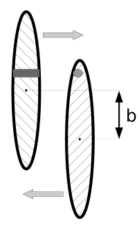
(b) Side View: $N_{\rm coll}$

Figure 5: Cartoons of collision geometry. The impact parameter is shown by ’b.’ 5(a) Front view of two symmetric nuclei colliding. The number of nucleons in the overlap region is known as $N_{\rm part}$. 5(b) Side view of the collision. The thickness of the nuclei is parametrized by the total number of binary collisions between nucleons, $N_{\rm coll}$. The light-grey circle represents a nucleon, while the dark-grey box shows the effective thickness of the nucleus seen by the nucleon.

Two variables that have been used to parametrize the centrality of nucleus-nucleus collisions are $N_{\rm part}$ and $N_{\rm coll}$. These parameters, while also not directly observable in an experiment, correlate well with impact parameter and have simple physical interpretations. Nucleons from one nucleus that collide (inelastically) with nucleons from the opposing nucleus are known as participants. The total number of participant nucleons in a collision is $N_{\rm part}$. As shown in Fig. 5(a), the overlap region in a collision is defined by the participating nucleons. Nucleons outside this region, that do not directly take part in the collision, are known as spectators. The number of binary collisions that the participating nucleons suffer is known as $N_{\rm coll}$. The number of binary collisions parametrizes the thickness of a nucleus seen by a nucleon in the opposing nucleus, as shown in Fig. 5(b). $N_{\rm coll}$ is commonly used to compare the results of AA collisions to those of nucleon-nucleon (NN) collisions since, in the absence of any nuclear effects, one would expect AA collisions to be simply a superposition of NN collisions. The details of determining the average $N_{\rm part}$ and $N_{\rm coll}$ for a set of collisions will be discussed in Sect. 2.

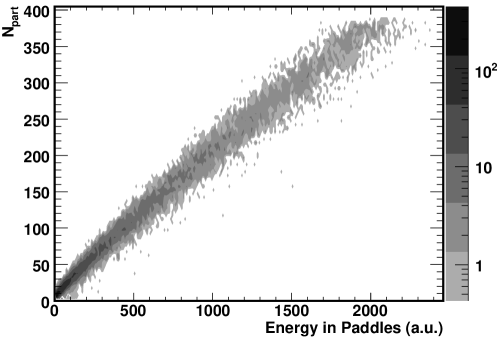
Figure 6: The amount of energy deposited into the Paddle detectors from Au+Au collisions correlated very well with $N_{\rm part}$ in the HIJING [61] model.

The average value of these parameters – $N_{\rm part}$ and $N_{\rm coll}$ – can be estimated for different classes of collisions using experimentally measured quantities. Intuitively, one would expect that a parameter like $N_{\rm part}$ (for example) should scale monotonically with the number of particles produced by a collision. Such scaling was found to hold in collision simulations, as shown in Fig. 6, where the multiplicity was measured using the Paddle detectors. It is possible to exploit this monotonic relationship by (a) grouping together collisions in which the measured quantity, e.g. the energy in the Paddles, is within some range and (b) using simulations to find the average of the desired parameter, e.g. $N_{\rm part}$, of the collisions in each group. In order to facilitate comparison of results between different experiments, and between experiment and theory, the groups of collisions are typically chosen to be specific fractions of the total inelastic collision cross section. See [92] for a detailed discussion of centrality in heavy ion collisions.

1 Centrality Cuts

The values of a measured quantity that are used to divide the data into groups of centrality classes are known as centrality cuts. These values are not known a priori; centrality cuts must be determined using collision data and the estimated efficiency of the detector for recording collisions usable in an analysis. Collisions that are usable in an analysis are those that not only pass the trigger, but also pass a user applied event selection. For example, a collision may occur 11 ${\rm cm}$ away from the IP and fire the dAuVertex trigger, but the same collision may not pass the event selection of an analysis that requires the collision vertex to be within 8 ${\rm cm}$ of the IP. Event selections used in the analysis presented in this thesis are described in Sect. 1.

With a perfectly efficient detector and event selection, centrality cuts could be determined in the most straight-forward way. A collision that produces, for example, a multiplicity greater than 90% of all other collisions would be known to have had a centrality greater than 90% of all collisions. Such a collision could therefore be placed into the top 10% fractional cross section centrality class (i.e. the 0-10% bin), since the chances of such a collision occuring is less than 10% of the total collision cross section. This reasoning was used to define the centrality cuts for a chosen measured quantity. One would simply divide the full distribution of the measured signals into centrality classes that directly correspond to the desired fractional cross section groups. For example, if one had recorded the energy in the Paddles in 200 events and wanted to find two centrality classes, 0-60% and 60-100% of the total cross section, the following procedure could be used. First, the events would be ordered by the recorded energy in the Paddles, from highest to lowest. Then the events would be counted, starting with the event that had the highest recorded energy in the Paddles, until 60% of all events had been counted. The value of the energy recorded in the Paddles of the last event counted, number 120, would be the desired centrality cut. That is, events that had more energy in the Paddles than this cut would be in the 0-60% group, while events that had less would fall into the 60-100% group.

Variable	Type	$\eta$ Coverage	Description
ERing	Multiplicity	$\pm(3.0,5.4)$	Energy in the Rings
EOct	Multiplicity	$(-3.2,3.2)$	Energy in the Octagon
EPCAL	Spectators	Beam	Energy of Proton Spectators

Table 1: Description of centrality variables used in this analysis.

An analogous procedure was adapted for finding centrality cuts in PHOBOS. Unfortunately, the PHOBOS detector was not a perfectly efficient detector. Fortunately, simulations of the detector could be used to estimate the efficiency of an event selection as a function of the desired centrality variable. The centrality variable refers to the measured quantity used to generate the centrality cuts; in the previous example, the centrality variable was the energy recorded in the Paddles. The centrality variables used in the analysis presented in this thesis were Energy in Rings (ERing), Energy in Octagon (EOct) and EPCAL. These variables are described in Table 1. The centrality cuts used in the analysis presented in this thesis were determined using several steps.

MC Scaling

The first step in finding centrality cuts was ensuring that the distribution of centrality variable signals in the Monte Carlo (MC) simulations corresponded to that of the recorded data. For such a correspondence to be expected, the event selection used in the analysis of data had to be equivalent to that placed upon the MC. See Sect. 1 for details on the event selections used in this analysis. With equivalent event selections placed on the data and MC, the overall shape of the distributions of the centrality variable signals in MC and data were expected to be the same. However, the absolute scale of signals in the MC and data were not necessarily equivalent. For example, a signal reported by the Paddle detector for a particular collision may be 5% lower in the simulations than the signal in the data would have been for the same event. As long as such a scaling factor is independent of the centrality of collisions, it does not affect the centrality cuts, since the cuts are based on fractions of the distribution.

While the absolute scale of the MC signals was not critical for finding the centrality cuts themselves, it was critical for finding the efficiency. This requirement stems from the fact that it was necessary to know the efficiency of the event selection for all values of the centrality variable in the data. Thus, before the efficiency could be determined, the centrality variable distribution in the MC had to be scaled such that it matched the same distribution in the data.

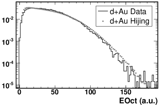
(a) EOct No Scaling

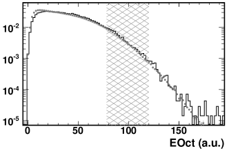
(b) EOct Scaled

Figure 7: Example of the scaling of EOct in MC. 7(a) Comparison of the normalized EOct distribution in the data and MC with no scaling. 7(b) Comparison of EOct in the data and MC, with EOct signals scaled down by 5.2% in the MC. The grey band shows the range of EOct used to determine the scaling factor.

It was assumed that for some region of sufficiently central events, the efficiency of the event selection should not change with centrality. In this region, then, the distribution of centrality variable signals in the MC could be scaled to match that of the data. This region was different for each centrality variable. The MC scale factor was determined in the following way. First, a test scale factor was chosen and the distribution of scaled signals from the MC was generated. This distribution and the data distribution were then independently normalized. A $\chi^{2}$ comparison between the scaled MC and the data was performed for signals in the chosen region. The region used for matching was a subset of the constant efficiency region, such that bins with low statistics were explicitly ignored. However, the same scaling factor was obtained when the full constant efficiency region was used to do the matching, as expected. This process was repeated for 50 different scaling values ranging from 90% to 120% (although a smaller range could have been used). The final scaling factor was chosen to be the one that yielded the best match according to the $\chi^{2}$ tests. An example of the scaling of MC, using EOct from Heavy Ion Jet Interaction Generator (HIJING) [61] simulations, can be seen in Fig. 7.

Efficiency

After the signal in the MC simulations had been scaled to match the signals seen in the data, the efficiency of the event selection could be determined. The desired efficiency would be a function of the centrality variable, and could be used to estimate the distribution of signals that would have been measured by a perfect detector, according to the relation

$$N_{ideal}(C)=\frac{N_{meas}(C)}{\epsilon(C)}$$ (2)

where $N_{ideal}(C)$ is the number of events recorded by an ideal detector in which the value of the centrality variable is $C$, $N_{meas}$ is the number of events measured in the actual data and $\epsilon$ is the estimated efficiency.

The efficiency of an event selection was estimated using the MC simulations. The basic procedure was simply to take the centrality variable distribution in the MC with the event selection and divide it by the same distribution in the MC without the event selection. One complication to this procedure arose due to the vertex requirement of an event selection. For example, an event selection that requires collisions to be within 2 ${\rm cm}$ of the IP might be 100% efficient for events satisfying this vertex requirement. However, if the MC simulations generated collisions that were randomly distributed within 4 ${\rm cm}$ of the IP, then the efficiency would be estimated as 50%, since half of the collisions generated by the MC would lie outside the vertex requirement of the event selection. This is clearly not the desired efficiency, since any efficiency value could be produced simply by changing the range of vertices in which collisions are simulated!

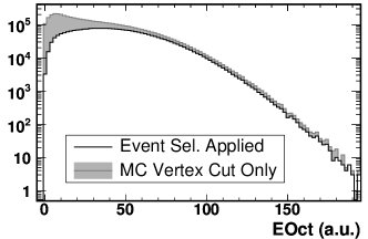
(a) With & Without Event Selection

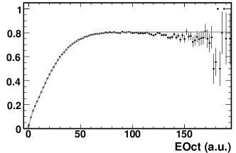
(b) EOct Efficiency

Figure 8: The efficiency of EOct from HIJING using the dAuSpectra event selection (see Sect. 1). 8(a) Scaled EOct distributions in the MC with the full event selection (black line) and with only a true MC vertex cut (grey shaded region). 8(b) The EOct efficiency profile is shown by the black points, while the fit is shown by the grey line.

The procedure used to estimate the efficiency for the analysis presented in this thesis was as follows. First, the scaled centrality variable distribution was produced for events in the MC that were generated within the vertex range required by the event selection. That is, rather than applying no event selection, a cut was placed only on the true MC vertex. This distribution was then divided by the scaled centrality variable distribution for events in the MC that passed the full event selection. The result of this ratio provided a profile of the efficiency, which was then fit with a function of the following form:

$$\frac{\alpha}{1+\exp\left(\beta_{0}-\gamma_{0}C\right)+\exp\left(\beta_{1}-\gamma_{1}C\right)+\exp\left(\beta_{2}-\gamma_{2}C\right)}$$ (3)

where $\alpha$, $\beta_{i}$ and $\gamma_{i}$ are fit parameters. Note that there was no physics motivation for this function; it simply provided a good fit to each efficiency profile without requiring any tweaking of initial parameter values or of parameter limits. The estimated efficiency function of EOct from HIJING using the dAuSpectra event selection (see Sect. 1) is shown in Fig. 8. It can be seen from this figure that $\sim 20\%$ of d+Au collisions are lost, even those having relatively large values of EOct. This inefficiency is due to the requirement that both T0 detectors be hit. It was traced to a combination of two effects: the small acceptance of the T0s and the relatively low number of particles produced at high pseudorapidity (on the deuteron side of the interaction).

Fractional Cross Section Cuts

The efficiency function was used to obtain an estimate of the centrality variable distribution in the absence of experimental biases. In other words, what would have been measured by an ideal detector. Using this distribution, it was possible to determine the fractional cross section cuts using the same method described in Sect. 1. The procedure used in the analysis presented in this thesis was as follows.

First, the unbiased centrality variable distribution was produced using the estimated efficiency. This was done by filling a histogram with the centrality variable signal from each collision event in the data that passed the event selection. Each entry in this histogram was weighted according to Eq. 2 as not one event, but rather as $1/\epsilon(C)$ events. The integral of this histogram gave the total number of events that would have been measured by an ideal detector, $N^{tot}_{ideal}$.

Then, fractions of $N^{tot}_{ideal}$ corresponding to the desired fractional cross section classes were computed. For example, the fractional cross section bins used in this analysis were, from most central to most peripheral, 0-20%, 20-40%, 40-70% and 70-100%. Since the widths of these bins were 20%, 20%, 30% and 30%, respectively, the most central bin contained $N^{central}_{ideal}=0.2{\times}N^{tot}_{ideal}$ events. More precisely, it should contain the $N^{central}_{ideal}$ most central events.

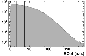
(a) EOct Unbiased Distribution

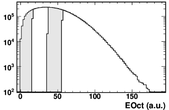
(b) EOct Centrality Bins

Figure 9: The centrality cuts for EOct from HIJING using the dAuSpectra event selection. 9(a) The efficiency corrected EOct distribution. The black lines show the centrality cut values. 9(b) The distribution of EOct in each fractional cross section bin. Alternating centrality bins are shaded to guide the eye. A step in the shading indicates the fraction of collisions in the EOct bin that belong to each centrality class.

Once the number of events in each centrality class was determined, the centrality cuts could be found. This was done by computing a cumulative sum of the entries in each bin of the unbiased histogram, starting from the highest bin. The bin which caused the sum to exceed $N^{central}_{ideal}$ was known to contain the first centrality cut value. For example, if $N^{central}_{ideal}=4$ events, the top bin of the unbiased histogram contained 2 events having a centrality signal between 90 and 100, and the next bin contained 5 events having a centrality signal between 80 and 90, then the centrality cut would have been between 80 and 90. In order to find the value of the centrality cut, it was assumed that the shape of the distribution was flat over the (small) width of the histogram bin:

$$K(G)=L_{i}+W_{i}\left(\frac{\sum_{j=top}^{j=i}\left(E_{j}\right)-N_{ideal}(G)}{E_{i}}\right)$$ (4)

where $K(G)$ is the cut value for the centrality group, $i$ is the histogram bin containing the centrality cut, $L_{i}$ is the lower edge of that bin, $W_{i}$ is the width of that bin, $E_{j}$ is the number of events contained in the $j^{th}$ histogram bin and $N_{ideal}(G)$ is the number of events that should be contained in the centrality group (i.e. $N^{central}_{ideal}$). Thus, for the previous example, Eq. 4 gives

$${}K({\rm central})=80+10\left(\frac{(2+5)-4}{5}\right)=86$$

This procedure was then repeated for each successively more peripheral centrality class. The centrality cuts generated in this way for EOct from HIJING using the dAuSpectra event selection (defined in Sect. 2) are shown in Fig. 9.

2 Centrality Parameters

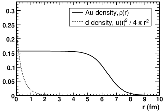
(a) Density Profiles

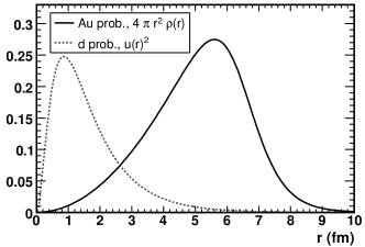
(b) Probability Profiles

Figure 10: 10(a) The nuclear density profiles used for gold (solid black line) and deuteron (dashed grey line) nuclei in the Glauber model. The variable $r$ shows the distance of each nucleon from the center of the nucleus. 10(b) The corresponding radial probability distributions for each nucleus.

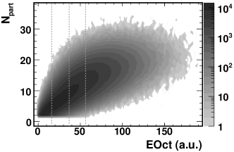
(a) $N_{\rm part}$ vs EOct

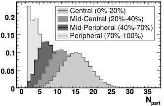
(b) $N_{\rm part}$ in Centrality Bins

Figure 11: The $N_{\rm part}$ distributions for the EOct centrality cuts. 11(a) $N_{\rm part}$ versus EOct in d+Au HIJING. The dashed grey lines show the centrality cut values. 11(b) The $N_{\rm part}$ distributions for each centrality class. Each distribution is (independently) normalized.

Once centrality cuts were obtained, they were applied to the MC simulations in order to study the properties of each centrality class. The distribution of parameters such as $N_{\rm part}$ and $N_{\rm coll}$ in each centrality class could be directly examined in the MC. Note that the distributions of such parameters were model dependent. In both the HIJING and AMPT [65] collision generators, a Glauber model was used to estimate the number of participant nucleons and binary collisions. In this model, the nucleons of each nucleus were distributed according to a density function. The nucleons were then assumed to travel in a straight line, undeflected by collisions. The probability that nucleons would interact was taken from the total inelastic p+p cross section of 41 ${\rm mb}$ (which is appropriate for $\sqrt{s_{\scriptscriptstyle{{\rm NN}}}}=200~{}\mbox{${\rm GeV}$}$) [93]. The number of participants and binary collisions were then directly counted. The simulations performed for this analysis used HIJING version 1.383, which modeled the structure of the deuteron using the Hulthen wave function [94]

$$u(r)=Ce^{-\alpha(2r)}\left(1-e^{-\mu(2r)}\right)$$ (5)

where $r$ is half the distance between the nucleons in the deuteron (the radius of the nucleus), $C$ is a constant that normalizes the probability distribution $u(r)^{2}$, $\alpha=(4.38~{}\mbox{${\rm fm}$})^{-1}$ and $\mu=(1.05~{}\mbox{${\rm fm}$})^{-1}$. The structure of the gold nucleus was modeled by a Woods-Saxon distribution,

$$\rho(r)=\frac{\rho_{0}}{1+\exp\left(\frac{r-R}{a}\right)}$$ (6)

where $r$ is the distance of a nucleon from the center of the nucleus,$R=6.38~{}\mbox{${\rm fm}$}$ describes the radius of the nucleus, $a=0.535~{}\mbox{${\rm fm}$}$ describes the diffuseness of the nuclear edge and $\rho_{0}$ normalizes the distribution. See Fig. 10 for a diagram of these probability densities.

For any given centrality class, the distribution of a parameter, such as $N_{\rm part}$, could be analyzed to find the average value of that parameter. This was done by constructing a histogram for each parameter and each centrality class. The histogram was then filled with the value of the parameter in every MC collision that belonged to that centrality class. The mean and RMS of the parameter could then be directly calculated from the histogram. The $N_{\rm part}$ distributions for the EOct centrality cuts, using HIJING and the dAuSpectra event selection, are shown in Fig. 11. If the event selection criteria were placed on the MC when generating the $N_{\rm part}$ distribution, then the average of the distribution would be a biased $N_{\rm part}$.

The bias introduced by the event selection could be undone either by (a) not applying the event selection or (b) using the efficiency (obtained according to Sect. 1) to correct for the bias. The latter method proceeded as follows. First, the efficiency of the event was determined by evaluating the efficiency function at the value of the centrality measure (i.e. EOct) in the event. Then, the event was weighted by the inverse of this efficiency. For example, an event with an efficiency of 50% would be counted as two collisions in the centrality parameter distribution. In this way, an unbiased distribution of the centrality parameter (i.e. $N_{\rm part}$) was constructed. Imposing the event selection on the MC and then using the efficiency to “remove” it may seem unnecessary for the simulations, when one could simply not impose any event selection. However, this type of efficiency weighting could be performed on the data (see Sect. 4), where an event selection was required. Therefore, this was the preferred method for finding an unbiased average $N_{\rm part}$ for a particular centrality cut bin.

3 PCAL Centrality

Centrality cuts derived from EPCAL signals were determined using a related, but modified procedure. This was necessary because a reliable model of the breakup of the gold nucleus was not implemented, so the Au-PCAL was not simulated in the HIJING or AMPT Monte Carlo. The procedure that was developed exploited the monotonic correlation in the d+Au data between the EPCAL signal, denoted $S_{\rm pcal}$, and the signal of another detector, denoted $S_{\rm corl}$ (EOct, for example).

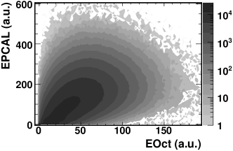
(a) EPCAL vs EOct

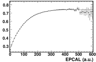
(b) EPCAL Efficiency

Figure 12: The EPCAL efficiency obtained from EOct. 12(a) The correlation between EPCAL and EOct in the d+Au data using the dAuSpectra event selection. 12(b) The EPCAL efficiency obtained using the known EOct efficiency.

The method relied on being able to derive an estimate for the efficiency of $S_{\rm pcal}$ using the known efficiency of $S_{\rm corl}$. This efficiency could then be used with the data to determine the centrality cuts. The centrality cuts were found in several steps. First, the distribution of $S_{\rm pcal}$ was generated for all events in the data that passed the chosen event selection. Next, a second $S_{\rm pcal}$ distribution was generated, for the same events, but in this distribution all events were not weighted equally. Rather, an event was weighted, according to Eq. 2, by $1/\epsilon_{corl}(S_{\rm corl})$. For example, if the correlated variable was EOct, then in each event the histogram would be filled with the EPCAL signal, weighted by a certain value. The value of the weight would be determined by evaluating the EOct efficiency function at the value of the EOct signal in the given event. The efficiency profile of $S_{\rm pcal}$ was then obtained by dividing the $S_{\rm pcal}$ distribution by the weighted distribution. This profile was then fit to obtain the efficiency function of $S_{\rm pcal}$. An example using EOct as the correlated signal is shown in Fig. 12.

The efficiency of $S_{\rm pcal}$ was used to find EPCAL centrality cuts in the normal way (see Sect. 1). Figure 13(a) shows the EPCAL centrality cuts obtained by using $S_{\rm corl}=$EOct with the dAuSpectra event selection. The estimation of the average value of a collision parameter, $P_{\rm coll}$ (such as $N_{\rm part}$), required a new procedure due to the lack of $S_{\rm pcal}$ in the simulations. Collision parameters were determined by exploiting both the correlation of $S_{\rm pcal}$ with $S_{\rm corl}$ and of $S_{\rm corl}$ with $P_{\rm coll}$. Two different procedures were developed to find the average values of collision parameters in EPCAL centrality cut bins. Since EPCAL centrality cuts could only be applied to d+Au data, and not to MC, both methods attempted to estimate the average $P_{\rm coll}$ of collisions in a centrality bin using the $S_{\rm corl}$ distribution of d+Au data collisions in that bin.

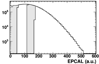
(a) EPCAL Cuts

(b) EOct in Central Bin

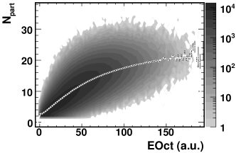
(c) $N_{\rm part}$ vs EOct Fit

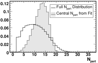
(d) $N_{\rm part}$ in Central Bin

Figure 13: $N_{\rm part}$ in EPCAL centrality bins obtained by the fit method. 13(a) The EPCAL centrality cuts from EOct with the dAuSpectra event selection. 13(b) The EOct distribution in the central EPCAL bin (grey histogram) compared to the full EOct distribution (black line). 13(c) The white line shows the fit to the $N_{\rm part}$ dependence on EOct in the MC. 13(d) The $N_{\rm part}$ distribution in the most central EPCAL bin (grey histogram) found using the fit method. Each distribution is (independently) normalized.

First, a naïve approach was taken by simply fitting the dependence of $P_{\rm coll}$ on $S_{\rm corl}$. The resulting function was then used to obtain an estimate of $P_{\rm coll}$ in a d+Au data event given the value of $S_{\rm corl}$ in the event. The function was obtained by first generating a two-dimensional histogram of $P_{\rm coll}$ versus $S_{\rm corl}$, such as the one shown in Fig. 11(a). From this, a one-dimensional profile of the $P_{\rm coll}$ dependence on $S_{\rm corl}$ was obtained. The position and error of each point in the profile distribution was determined by the mean and RMS of $S_{\rm corl}$ bins in the two-dimensional histogram. The profile was then interpolated by a $3^{rd}$ degree polynomial spline with 100 knots. Figure 13(c) shows the interpolated function obtained for $S_{\rm corl}=$EOct and $P_{\rm coll}=N_{\rm part}$ with the dAuSpectra event selection. From the interpolated function, it was possible to estimate the value of $P_{\rm coll}$ given the value of $S_{\rm corl}$ in a d+Au collision. Thus, $P_{\rm coll}$ distributions could be obtained for each EPCAL centrality bin. The result of this method for the most central EPCAL bin is shown in Fig. 13(d).

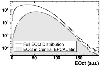
(a) EOct in Central Bin

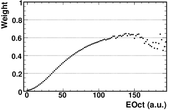
(b) EOct Weights in Central Bin

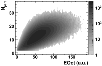
(c) $N_{\rm part}$ vs Weighted EOct

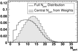
(d) $N_{\rm part}$ in Central Bin

Figure 14: $N_{\rm part}$ in the most central EPCAL bin obtained by the weighting method. 14(a) The EOct distribution in the central EPCAL bin (grey histogram) compared to the full EOct distribution (black line). 14(b) EOct weights in the central bin, obtained by taking the ratio of EOct in the central bin to the full EOct distribution. 14(c) The $N_{\rm part}$ dependence on EOct with EOct values weighted by their probability of occurring in the most central EPCAL bin. 14(d) The $N_{\rm part}$ distribution in the most central EPCAL bin (grey histogram) found using the weighting method. Each distribution is (independently) normalized. Compare to Fig. 13(d).

The second approach was to estimate the correlation between $P_{\rm coll}$ and $S_{\rm corl}$ in an EPCAL centrality bin. This was done by weighting the $S_{\rm corl}$ distribution in the MC. Two-dimensional histograms of $P_{\rm coll}$ versus $S_{\rm corl}$ for all EPCAL centrality bins were constructed. Each histogram was then filled using every MC event, but all collisions were not weighted equally. Instead, a MC event was weighted by the likelihood that a d+Au collision, in the chosen EPCAL centrality bin, would be found having the same value of $S_{\rm corl}$. The weighted correlation between EOct and $N_{\rm part}$ in the most central EPCAL bin is shown in Fig. 14(c). The likelihood weights were obtained in a simple manner. For each EPCAL centrality bin, the distribution of $S_{\rm corl}$ in that bin was divided by the full $S_{\rm corl}$ distribution (see Fig. 14(a) and 14(b)). The average value of $P_{\rm coll}$ in a EPCAL centrality bin was then estimated by projecting the two-dimensional histogram onto the $P_{\rm coll}$ axis and calculating the mean, as shown in Fig. 14(d).

4 Deuteron-Nucleon Tagging

1 The Deuteron

The mass of a nucleus is always less than the sum of the masses of the individual nucleons which make up the nucleus. This can be understood using the famous formula $E=mc^{2}$. For a nucleus or a nucleon at rest, its mass is its total energy, and in order for the nucleus to exist, it must be energetically favorable for the nucleons to bind together. Thus, the total energy (i.e. mass) of a nucleus at rest must be less than the sum of the energy (mass) of each individual nucleon. This difference in mass is known as the binding energy of the nucleus,

$$B(A,Z)=c^{2}\left(ZM_{p}+(A-Z)M_{n}-M(A,Z)\right)$$ (7)

where $A$ is the number of nucleons in the nucleus, $Z$ is the number of protons, $M_{p}$ is the mass of a proton, $M_{n}$ is the mass of a neutron, $M(A,Z)$ is the mass of the nucleus and $B(A,Z)$ is the binding energy of the nucleus.

The deuteron is a very weakly bound nucleus. While all nuclei heavier than Neon ($A=10$) have a binding energy above 7.4 ${\rm MeV}$ per nucleon [96], the deuteron has only

$$B(A,Z)/A =c^{2}\left(M_{p}+M_{n}-M_{d}\right)/2$$ (8)

$$=\left(938.27~{}{\mbox{${\rm MeV}$}}+939.57~{}{\mbox{${\rm MeV}$}}-1875.61~{}{\mbox{${\rm MeV}$}}\right)/2$$

$$=1.11~{}{\mbox{${\rm MeV}$}}$$

This weak binding energy has two consequences that are relevant to the analysis presented in this thesis. First, as can be seen in Fig. 10, it is quite possible for the nucleons of a deuteron to be found relatively far apart. If the deuteron is in such a state when it collides with a gold nucleus, then it is possible that only one nucleon will actually participate in the collision. The second consequence is that the remaining spectator nucleon can emerge from the collision relatively unperturbed. Thus, such a collision is nearly equivalent to the collision between a single nucleon and a gold nucleus.

These types of p+Au and n+Au collisions were identified in the d+Au data by actively looking for spectator nucleons from the deuteron. If, in a d+Au collision, a spectator neutron was observed and no spectator proton was observed, then it was inferred that the proton interacted in a p+Au collision. Similarly, if the only deuteron spectator observed was a proton, then the neutron must have interacted in a n+Au collision.

2 Identifying Nucleon-Nucleus Collisions

The deuteron spectators were measured in PHOBOS using the d-PCAL and d-ZDC detectors. Qualitatively, a collision in which the d-PCAL recorded a hit and the d-ZDC did not was labeled a n+Au interaction (and vice-versa). A hit in each detector was defined as a signal that was within certain limits. These limits could have been chosen tightly, so that only signals underneath the neutron or proton peaks were used, but tight cuts would have rejected a large number of collisions that were otherwise acceptable for analysis. However, if the limits were too loose, then the fraction of mis-identified nucleon-nucleus collisions would increase. The goal, then, was to chose limits that would reject the fewest number of collisions while still maintaining as pure a signal as possible.

Because the calorimeters were not simulated in the d+Au MC, the purity of different signal cuts could not be directly studied. Instead, the shapes of certain centrality variable distributions, such as ERing, were studied in the d+Au data. This study was motivated by the bias that tagging a deuteron spectator introduces on centrality: a d+Au collision in which only one nucleon from the deuteron interacts is likely to have a larger impact parameter than an average d+Au collision. Thus, the ERing distribution in a nucleon-nucleus collision should be biased toward more peripheral collisions when compared to the ERing distribution of d+Au.

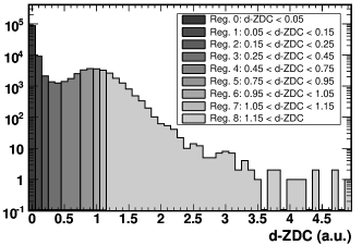
(a) d-ZDC Regions

Figure 15: Studying the impact of d-ZDC cuts on the shape of a centrality variable. 15(a) The regions of d-ZDC used in the study. 15(b) The normalized ERing distributions when no neutron is present (grey histogram) and when a neutron is clearly present (dark grey line). 15(c) The ratio of ERing in each region to that of region 5, which is under the neutron peak. The color of the lines follow the same color scheme as used in 15(a). Note that region 0, shown by the darkest grey line, in which no neutron is observed, has a significantly different shape from all other regions.

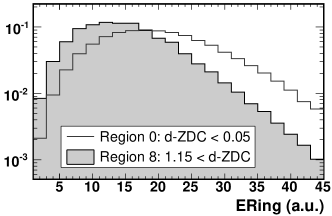
(b) ERing in d-ZDC Regions

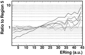
(c) Ratio: ERing in Each Reg. to Reg. 5

By studying the shape of centrality distributions for different regions of d-ZDC and d-PCAL signals, it was possible to measure the bias introduced by selecting nucleon-nucleus collisions. Figure 15(a) shows such a study of ERing distributions, for different regions of d-ZDC signals. As can be seen in Fig. 15(b), the ERing distribution from collisions with the largest signals in the d-ZDC detector is indeed biased toward peripheral collisions when compared to the ERing distribution from collisions with no signal in the d-ZDC. The ratio of the latter distribution, ERing in region 0, to the distribution of ERing from collisions with d-ZDC signals that are under the neutron peak (region 5) is clearly visible in Fig. 15(c). This shows that collisions with a d-ZDC signal below 0.05 units can not be identified as p+Au interactions. It also shows that the centrality bias of collisions in regions 3 and above are roughly the same.

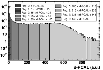
(a) d-PCAL Regions

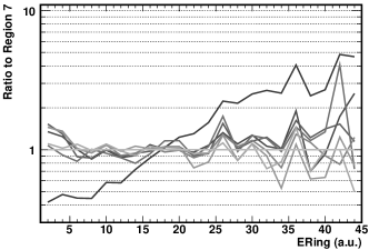
(b) Ratio: ERing in Each Reg. to Reg. 7

Figure 16: Studying the impact of d-PCAL cuts on the shape of a centrality variable. 16(a) The regions of d-PCAL used in the study. 16(b) The ratio of ERing in each region to that of region 7. The color of the lines follow the same color scheme as used in 16(a). Note that region 0, in which no proton is observed, has a significantly different shape from all other regions.

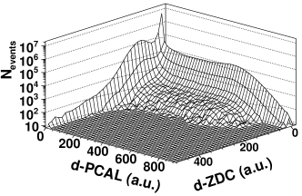
(a) d-PCAL vs d-ZDC

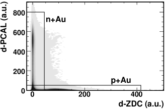
(b) d-PCAL vs d-ZDC with Tag Cuts

Figure 17: The d-PCAL signal versus the d-ZDC signal. Note that in both plots, only bins that contain more than 6 collisions are shown. 17(a) A surface representation that shows the shape of each distribution. 17(b) A contour representation that shows the lack of correlation between the two calorimeters. The boxes (at high d-PCAL, low d-ZDC and vice-versa) show the regions in which collisions were identified as a p+Au or n+Au collision.

A similar study for regions of d-PCAL signals is shown in Fig. 16. For the d-PCAL, it is even more apparent that regions showing any amount of signal in the calorimeter have a similar centrality bias – suggesting that this signal is indeed due to a spectator from the deuteron. Therefore, the cuts were placed at the high edge of the pedestal peak, more than $6~{}\sigma$ above the pedestal (taking the average noise of a channel as $\sigma$). The final nucleon-nucleus tagging cuts are shown in Fig. 17.

3 Centrality of Nucleon-Nucleus Collisions

Due to the lack of simulations of the calorimeters, it was not possible to obtain the efficiency of an event selection that implemented d-PCAL or d-ZDC signal cuts. Thus, no centrality cuts specific to the tagged p+Au or n+Au data sets were generated. Instead, the same cuts used for the untagged d+Au data were applied to the p+Au and n+Au collision data. Of course, a centrality cut that selected the top 20% of the d+Au cross section would select a different percentage of the p+Au (or n+Au) cross section. Furthermore, without knowing the efficiency of the tagging procedures, it was not possible to determine the percentage cross section of centrality bins in the tagged p+Au and n+Au data. However, it was possible to obtain the average of MC parameters, such as $N_{\rm part}$, in p+Au and n+Au centrality bins.

The average value of MC parameters in p+Au and n+Au centrality bins were found using all simulated p+Au and n+Au collisions. Ideally, one would not use all p+Au and n+Au collisions, but only those that generated signals in the calorimeters which would pass the nucleon tagging cuts. Since the calorimeters were not simulated, this was not possible. Instead, the true MC information about which particles were in fact spectators was used. This procedure assumed that the distribution of a MC parameter, such as $N_{\rm part}$, was the same in tagged p+Au (n+Au) collisions as it was in true p+Au (n+Au) collisions. However, these distributions could be different if some events that passed the tagging cuts were not really p+Au (n+Au) collisions or if the chance that a spectator would deposit energy in a calorimeter depended on the centrality of the collision. Note that the chance of observing a spectator is distinct from the chance of producing a spectator, which certainly depends on centrality. Thus, the validity of using true MC information to select p+Au and n+Au collisions in the simulations rested on three assumptions. First, that it was not possible for a nucleon of the deuteron to both interact with the gold nucleus and to deposit a measurable amount of energy into one of the calorimeters. Second, that if such a nucleon did not interact, it would be observed by the calorimeters with some efficiency, but that this efficiency was independent of the centrality of the d+Au collision. Finally, that the d-PCAL and d-ZDC detected only deuteron spectators.

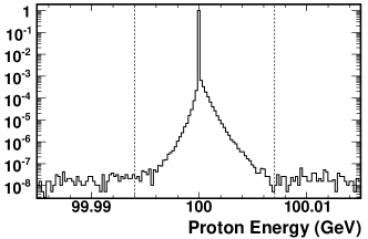
(a) Proton Energy Cut

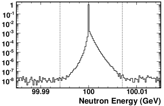
(b) Neutron Energy Cut

Figure 18: The energy cuts used to find spectators in simulated d+Au collisions are shown by the dashed grey lines. 18(a) The energy of protons in the HIJING MC. 18(b) The energy of neutrons in the HIJING MC.

Given these assumptions, a simple method was developed to find spectators in simulated collisions. The procedure was to use a restrictive energy cut: any proton or neutron having between 99.994 ${\rm GeV}$ and 100.007 ${\rm GeV}$ of energy was assumed to be a spectator. Spectators were identified as coming from a particular nucleus by their momentum in the beam direction; positive $p_{z}$ implied a deuteron-spectator and negative $p_{z}$ implied a gold-spectator. The distributions of proton and neutron energy in HIJING simulations are shown in Fig. 18. For HIJING, which reported the number of participants of each nucleus (but not separately for neutrons and protons), this energy cut almost always yielded the correct number of deuteron spectators. A value different from that reported by HIJING occurred only once in every 500,000 collisions.

The same procedure was used for the AMPT simulations. In the original AMPT model, dated August 18, 2003, the number of deuteron and gold participants reported did not come directly from the Glauber model. Instead, some kinematic cuts were used to identify the spectators, thereby determining the number of participants. In order to obtain consistent results between AMPT and HIJING, the AMPT model used in the analysis presented in this thesis was altered. In this altered AMPT, the number of participants of each nucleus was taken directly from the Glauber model (as run by the HIJING portion of the full AMPT model). However, the energy cut could not be used to reproduce the number of participants reported by the Glauber model. This was due to the hadron transport model [67] incorporated in AMPT, which was used to model the interactions between hadrons formed after a d+Au collision. In this model, it was possible for hadrons that did not interact in the initial collision between the nuclei (i.e. spectators in the Glauber model) to later participate in the final stages of the collision. Note that the energy cuts could also not reproduce the number of participants reported by the original AMPT model. This was due to the fact that the original AMPT counted the number of participants prior to running the hadron transport model. Nevertheless, the discrepancy between the number of deuteron participants reported by the Glauber model and the number that could be identified using the energy cuts was a feature of the AMPT model. It did not invalidate the procedure used to identify the deuteron participant nucleons.

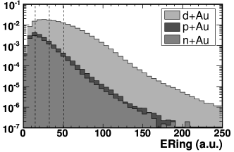
(a) ERing Distributions

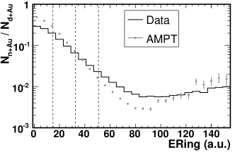
(b) n+Au / d+Au in Data and MC

Figure 19: 19(a) The ERing distribution of d+Au, n+Au and p+Au interactions as observed in the data. 19(b) The ratio of the ERing distribution in n+Au to that of d+Au for both the data (black line) and the AMPT simulations (grey points).

The ERing distribution observed in the data is presented in Fig. 19(a) for d+Au, p+Au and n+Au collisions. The dashed vertical lines show the centrality cut positions. The $\sim 35\%$ difference between the number of p+Au and n+Au collisions observed, which was found to be independent of centrality, reflects the different efficiencies of the two calorimeters. It can be seen that the tagged nucleon-nucleus interactions were biased toward more peripheral collisions. This was studied in more detail by looking at the ratio of the ERing distribution in n+Au to the ERing distribution in d+Au, as shown in Fig. 19(b). That this ratio is not constant as a function of ERing is a consequence of the peripheral bias of tagged n+Au collisions. Such a bias was expected, as the chance of one of the nucleons of the deuteron avoiding a collision with the gold nucleus should decrease with decreasing impact parameter. To test whether this bias was the same in the simulations as it was in the data, the analogous ratio was determined for n+Au and d+Au interactions in AMPT, also shown in Fig. 19(b). This comparison revealed that the bias was indeed qualitatively similar in the mid-peripheral and mid-central bins. However, the relative shape of the ERing distribution of n+Au and d+Au interactions in AMPT differed from that of the data. Thus, the centrality of “central” n+Au collisions was qualitatively different in AMPT as compared to the data. Therefore, the average number of participants of a central nucleon-nucleus interaction may not have been estimated accurately by the simulations. Some possible implications of this discrepancy will be discussed in Sect. 1.

The simulations were also used to obtain a rough estimate of the tagging efficiency. Due to the discrepancy between data and simulation, these efficiencies were not used in the analysis presented in this thesis. As long as these efficiencies are independent of centrality, the would not impact the measurements performed in this thesis. Nevertheless, they were estimated by comparing fraction of tagged collisions observed in the data to the fraction of nucleon-nucleus collisions that occurred (and passed the event selection) in the simulations. This comparison gave an estimate of the average efficiency with which a nucleon-nucleus collision would be successfully tagged. It was found that $\sim 63\%$ of p+Au interactions and $\sim 46\%$ of n+Au interactions would be tagged using the procedure described in Sect. 2.

Chapter 4 Particle Reconstruction

Calibrated signals in the Spectrometer detector were used to measure the properties of individual (charged) particles. The charge and momentum of a particle could be determined by the curvature of its trajectory through the magnetic field. The full trajectory of a particle consisted of two distinct sections, as each particle followed a straight path before entering the magnetic field and a curved path while traveling through the field. Particles were measured by first finding the straight path followed by the particle, then tracking its movement through the magnetic field and finally fitting the two sections together. All tracking procedures were performed separately for the two Spectrometer arms. An example of tracked particles in a Au+Au collision is shown in Fig. 1.

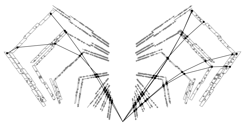
Figure 1: Tracked particles in a central Au+Au collision. The grey dots show all merged hits in the Spectrometer. The black dots show the hits assigned to a track. The black lines are straight line segments that connect the hits on a given track, to guide the eye.

1 Straight Track Finding

The first step in reconstructing the trajectories of particles in a d+Au collision was to locate all straight tracks. A straight track was the path taken by a particle in the first six layers of a Spectrometer arm. As seen in Fig. 5(b), the strength of the magnetic field in this region was negligible, so it did not significantly affect the motion of charged particles. Due to the small acceptance of the PHOBOS Spectrometer and the low multiplicity of d+Au collisions, only one straight track was observed in an average dAuVertex triggered collision event.

Straight tracks were found in a relatively simple manner. First, all combinations of hits on the first and fourth layers of each arm were taken as candidates for straight tracks. Next, each track candidate was extrapolated back to $x=0$, the nominal horizontal position (transverse to the beam direction) of collisions in the detector. This was done so that the distance of the track origin from the beam orbit could be computed. The beam orbit was observed to have no slope in either the horizontal or vertical plane. Since tracks in the Spectrometer acceptance were also very nearly horizontal, only the vertical distance between the track origin and the beam orbit was considered. If the height of the track (at $x=0$) was more than 2.5 ${\rm cm}$ above or below the beam orbit position, then the track was rejected as not having come from the d+Au collision.

Then, for each candidate, an attempt was made to find hits on the remaining layers that could be associated with the track. For a given layer, hits within 2 ${\rm mm}$ of the track candidate were examined, and the hit closest to the track was then associated with that track. For hits on the fifth and sixth layers, this constraint was relaxed in the vertical direction to account for the height of the pad, which was larger than 2 ${\rm mm}$. Of course, hits on each layer could not be found for every two-hit track candidate, since every candidate was not necessarily representative of a physical particle. To increase the probability that a straight track was in fact a reconstruction of the trajectory of a physical particle, it was required that each straight track have a hit on at least four layers of the Spectrometer.

This procedure was repeated for a different set of track candidates: those formed by the combination of hits on the third and fourth layers. For these candidates, the first two layers of the spectrometer were ignored completely. The only hits to be associated with these tracks were those found on the fifth and sixth layers of the Spectrometer. However, the requirements that each straight track extrapolate back to within 2.5 ${\rm cm}$ of the beam height and have hits on at least four layers of the Spectrometer were maintained.

The direction of a straight track was found by performing a least-squares fit of a straight line to the hits associated with the track. Two linear fits were performed: one in the $x-z$ (horizontal) plane and one in the $y-z$ (vertical in the beam direction) plane. The horizontal fit used only those hits in the first four layers, to reduce effects of the magnetic field. The vertical fit used all hits associated with the track. The fit procedure was performed each time a new hit was associated with the track. This allowed the best estimate of the trajectory to be used when searching for hits close to the track in successive layers.

2 Curved Track Finding

The curved trajectory of a particle was reconstructed by chaining together track segments that shared common physical properties. Combinations of two hits on successive layers of a Spectrometer arm were used to form the track segments. A Hough transform procedure [97] was used to determine the polar angle, $\theta$, and the inverse of the momentum, $1/p$, of a particle with a trajectory containing the track segment. The polar angle was defined as the angle between the beam line and the trajectory of the particle at its point of origin (the collision). Because the track segments were short, straight and used for performing a Hough transform, they were referred to as Hough-sticks.

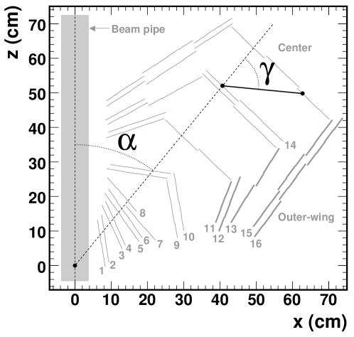
Figure 2: The angles describing a Hough-stick, in this case in the central region between layers 14 and 15, shown as the solid black line. The bold sensors represent the outer-wing. The corresponding angled sensors near the beam form the inner-wing (not labeled).

	Central Region	Outer-Wing Region
Stick	Layers Paired	Layers Paired
A	9 - 10	9 - 10
B	10 - 11	10 - 11
C	11 - 13	11 - 13
D	13 - 14	13 - 15
E	14 - 15	15 - 16

Table 1: Layers used when pairing hits to form Hough-sticks. The Spectrometer geometry, shown in Fig. 2, motivated the layers that were (and that were not) used in the Hough tracking.

The first step in chaining together Hough-sticks was to generate the sticks themselves. This was done by pairing a hit on a specific layer of the Spectrometer with another hit on a successive layer. In total, six hits were used to form the five sticks of a Hough-chain. Two separate methods of pairing hits were used: one that could find sticks only in the central part of the spectrometer, and another that could find sticks in the outer-wing (away from the beam). Figure 2 shows the distinction between the center and outer-wing sections of a Spectrometer arm. Table 1 shows the layer pairs used to form Hough-sticks in the central and outer-wing regions of the Spectrometer. All combination of hits on these layers were used to form as many Hough-sticks as possible.

Next, the physical properties of each Hough-stick were determined. This was done by calculating two angles: $\alpha$, the polar angle of the hit closest to the beam, and $\gamma$, the relative angle between the two hits [98]. These angles are shown in Fig. 2 for a Hough-stick connecting layers 14 and 15 of the central region of the Spectrometer.

The vertex point used to define $\alpha$ did not come from the OctDe vertexing algorithm, due to the poor resolution of this vertexing procedure. Instead, for d+Au collisions, the vertex was taken to be the intersection of a straight track and the beam orbit. That is, for each straight track candidate, the vertex was assumed to be the interaction of the track and the beam orbit. The full curved tracking was then run with this assumption. This process was then repeated for each straight track. Finally, any duplicate tracks resulting from running the tracking multiple times were explicitly removed, as described in Sect. 3.

Note that the angles $\alpha$ and $\gamma$ simply described the location of the two hits at the ends of the Hough-stick; they did not describe properties of the particle track. That is, $\alpha$ was the polar angle of the first hit in the stick, while $\theta$ was the polar angle of the track (at its origin). The physical parameters, $\theta$ and $1/p$, of a particle whose trajectory would contain the hits at the ends of the Hough-stick were obtained using a simple lookup table, called a Hough-table.

Hough-tables were stored as histograms with $20~{}\alpha$-bins and $20~{}\gamma$-bins. There was one Hough-table for each combination of: (a) the five pairs of layers used to form sticks, (b) the two regions of the Spectrometer used to find sticks (center and outer-wing), (c) the two electric charges of charged particles, (d) the 50 vertex regions of 0.5 ${\rm cm}$ width between $z=-15~{}\mbox{${\rm cm}$}$ and $z=+10~{}\mbox{${\rm cm}$}$, and (e) the two physical parameters that were to be looked up. The z-axis of a Hough-table stored the value of the physical parameter in question (such as $\theta$) that a track with a given $\alpha$ and $\gamma$ would have. Since the histograms were discretely binned, the value of the physical parameters were directly accessible only for values of $\alpha$ and $\gamma$ at the center of a bin. Polynomial fits were used to extrapolate between bin centers. For the $\theta$ lookup tables, the polynomial fits were performed along the $\alpha$ direction, but the lookup was still discrete in the $\gamma$ direction. For the $1/p$ lookup tables, the polynomial fits were performed along the $\gamma$ direction, but the lookup was discrete in the $\alpha$ direction.

The Hough-tables were filled using MC simulations of single tracks. For this purpose, only charged pions entering one Spectrometer arm were simulated. In addition, only one orientation of the magnetic field was used. These simplifications were implemented under the valid assumptions that (a) the vast majority of particles produced in nucleus-nucleus collisions at RHIC were pions, (b) one Spectrometer arm was a mirror image of the other (about the beam line), and (c) the trajectory of a positive pion in one magnetic field orientation was the same as that of a negative pion (with equivalent momentum) in the opposite field orientation. The range of the $\alpha$ and $\gamma$ axes in each Hough-table were determined dynamically by the range of values observed in the simulations. For a given particle, the appropriate cell of a Hough-table was filled with either $1/p$ or $\theta$. Each cell of the Hough-table was then normalized by the number of particles that had been used to fill that cell. Thus, the value of $\theta$ or $1/p$ stored in a Hough-table was ultimately the average parameter for particles in that cell. In a similar manner, tables were constructed to store the average relative error of $1/p$ and $\theta$. For a given simulated particle, the relative error was calculated as the difference between the true value of the parameter of the particle and the average value of the parameter for the cell in the table, normalized by the true value.

Once the physical parameters $\theta$ and $1/p$ had been determined for each Hough-stick, it was possible to form a Hough-chain. First, Hough-sticks that shared hits – that is, the outer hit of one stick was the same as the inner hit of another stick – were considered for chaining. Since a single particle would have had definite values of $\theta$ and $1/p$, all Hough-sticks formed by the hits of a single particle should have had the same physical parameters. Thus, if $\theta$ and $1/p$ for each of the two sticks being considered were similar, then they were chained together. A physical parameter of one stick was said to be similar to that of a second stick if the difference between them was not more than six times the error on that parameter. The error on the parameter was calculated by summing quadratically the error of the parameter on each stick.

Finally, a series of checks were performed on the Hough-chain to ensure its quality. First, only complete chains were kept; any chain with less than five sticks was rejected. Then, requirements were placed on the vertical displacement of the hits on a chain to reject chains that did not follow a smooth trajectory in the vertical direction. Next, chains formed by hits that had excessive differences in deposited energy were rejected. Finally, a $\chi^{2}$-statistic (see Eq. 10) was calculated for the Hough-chain, taking into account the errors on each Hough-stick as well as fluctuations in the positions of hits away from the expected particle trajectory in the $x-z$ plane. Hough-chains with large values of $\chi^{2}$ were rejected as having a low probability of representing a physical particle.

3 Momentum Determination

The first step in finalizing the trajectory of an observed particle, and measuring its momentum, was to match the curved section of the trajectory with the straight section. Then, all hits on the full track were fit numerically to obtain the best measurement of the trajectory and physical properties of the particle that generated the hits. Finally, a check was performed to clean up duplicate tracks that shared a large number of hits and were most likely reconstructions of the same physical particle.

1 Full Track Construction

A full collection of hits that could have been caused by a single particle was constructed by matching straight tracks with Hough-chains. The first step in this procedure was to find every straight track which could be fit to a straight line with a $\chi^{2}$-probability greater than 1%. Next, each of these straight tracks were compared to all the Hough-chains in the collision event. Four requirements had to be met for a straight track to be joined with a Hough-chain. The first requirement was that the polar angles of the straight track and the Hough-chain did not differ by more than 15 ${\rm mrad}$. The second requirement was a very loose one. It ensured that the difference between the mean deposited energy (per ${\rm cm}$ of silicon) of hits in the straight track and the mean $\mathit{dE}/\mathit{dx}$ of hits in the Hough-chain be less than 80% of the average $\mathit{dE}/\mathit{dx}$ of all hits on the track. The next two requirements imposed constraints on the distances of hits from the expected trajectory of a particle. The $\chi^{2}$-statistic described in Sect. 2 was again checked, to further reject chains that had a low probability of representing a particle. The final requirement ensured that the full track would follow a straight line in the vertical direction. First, the vertical slope of the straight track was computed. Then, the vertical deviation of hits in the Hough-chain from this straight line were used to compute a $\chi^{2}$ sum, labeled $\chi^{2}_{y}$. The $\chi^{2}_{y}$ per degree of freedom (in this case, the six hits on the chain) was required to be less than 5. If, and only if, all of these requirements were met, then the straight track and Hough-chain were combined together into a full track, known as a SpecTrack. The constraints enforced during track matching were designed to be loose requirements, to produce as many reasonable track candidates as possible.

2 Trajectory Fitting

The true trajectory and momentum of a particle was estimated using the hits on the SpecTrack. The time-honored method for doing this is to fit a simple, analytical form of the trajectory to the hits. However, due to the complexity of the magnetic field shape in the region of the Spectrometer arms, this procedure was not used in PHOBOS. Instead, the trajectory of a particle was estimated numerically using the measured strength of the magnetic field at a large number of points (this map is shown in Fig. 5(b)). The charge, momentum and point of origin of the SpecTrack obtained from the track matching was used to simulate the trajectory of a pion through the magnetic field. This trajectory simulation proceeded by calculating the location and momentum vector of the particle at each step along its path. For SpecTracks in the central region of the Spectrometer, the distance between steps along the trajectory was fixed at 10 ${\rm cm}$. Since the simulation of particles through the magnetic field was computationally intensive, large step sizes were chosen in this region to reduce computing time. However, when the particle would pass through a region in which the magnetic field was changing, the step size was reduced by half to improve the accuracy of the simulation. Since SpecTracks in the outer-wing of the Spectrometer could spend a significant amount of time in such a region, a variable step size was implemented for these tracks. The step size of tracks in the outer-wing depended on the momentum of the particle as $2.5~{}\mbox{${\rm cm}$}+k\cdot p$, where $p$ is the momentum of the particle and the constant $k$ was taken to be simply $1~{}\mbox{${\rm cm}$}/\mbox{${\rm GeV}$}$.

The resulting trajectory could then be used to calculate a $\chi^{2}$ statistic that accounted for the deviation of hits on the SpecTrack from the expected particle position. These deviations, known as residuals, were used to reject SpecTracks whose hits were located too far from the expected particle trajectory. However, the trajectory resulting from the numerical estimation was that of an ideal particle. This was due to the relative simplicity of the numerical simulation. Effects such as energy loss inside the silicon and deflections of a particle passing through some material, known as multiple scattering, were not considered. Thus, it was expected that the trajectory of a physical particle could differ from that of an ideal particle with the same charge, origin and momentum. These differences would obviously affect the $\chi^{2}$ computed for a SpecTrack and had to be taken into account. For SpecTracks that passed the residual cut, this was done by looking up the expected deviations in a covariance, or error, matrix. Diagonal elements of this matrix stored the deviation of physical particles from ideal particles at a particular layer of silicon. Off-diagonal elements stored the correlation between deviations in different layers of silicon.

Parameter	Minimum	Maximum	Number of Bins
Charge	-1 $e$	+1 $e$	2
$1/p$	0.1 $(\mbox{\rm GeV$\kern-1.49994pt/\kern-1.19995ptc$})^{-1}$	10 $(\mbox{\rm GeV$\kern-1.49994pt/\kern-1.19995ptc$})^{-1}$	40
$\theta$	0.25 ${\rm rad}$	1.75 ${\rm rad}$	30
$z_{0}$	-20 ${\rm cm}$	10 ${\rm cm}$	60

Table 2: Bins of physical parameters used to construct a covariance matrix. ‘$z_{0}$’ refers to the particle’s point of origin along the beam direction.

The covariance matrix was constructed prior to data-taking using simulations of physical particles. First, the physical parameters of a pion were chosen: charge, point of origin, total momentum and polar angle. These parameters were then fed into the numerical trajectory estimating procedure described above, to obtain the path of an ideal particle. Next, a pion with the same physical parameters was fully simulated, taking effects such as energy loss and multiple scattering into account. From these, the deviations between the ideal and physical particle trajectories were computed. A different covariance matrix was constructed for each combination of the different physical parameters used to simulate particles. Similar values of physical parameters were binned together to generate a covariance matrix, as described in Table 2. In each bin, 5000 sets of physical parameters were chosen randomly, and each set was then fed into the numerical and full particle simulations.

Using the simulated ideal particle trajectory together with the appropriate covariance matrix, the $\chi^{2}$ of a particular SpecTrack and momentum hypothesis was computed. This process was repeated iteratively to find the momentum vector that minimized the $\chi^{2}$ of a SpecTrack. More precisely, the physical parameters varied during the fitting routine were (a) the inverse of the total momentum $1/p$, (b) the polar angle $\theta$, (c) the azimuthal angle $\phi$, (d) the point of origin along the beam $z_{0}$, and (e) the point of origin in the vertical direction $y_{0}$. In order to minimize $\chi^{2}$ while varying all five parameters, a simplex minimization technique was adopted. This technique chose 6 points in the 5-dimensional parameter space at which $\chi^{2}$ was calculated. The shape created by drawing connecting lines between the points is known as a simplex. The points were randomly chosen around the initial physical parameters determined by track merging. The point with the largest $\chi^{2}$, and therefore worst fit, was moved through the opposite face of the simplex in such a way as to reduce the volume of the simplex. This procedure was then repeated, allowing the simplex to fall into the region of lowest $\chi^{2}$. Minimization was stopped when the $\chi^{2}$ calculated at the points of the simplex did not deviate by more than 0.001 units. See [99] for more information on simplex minimization techniques.

3 Duplicate Track Rejection

The final step in reconstructing particles in the Spectrometer was to find and clean up duplicate tracks. Duplicate tracks were groups of SpecTracks that were thought to have a high probability of all describing the same physical particle. First, all tracks with less than eleven hits were rejected. Then, to find duplicate tracks, each pair of the remaining SpecTracks was compared. If a pair of tracks shared more than two hits, then they were assumed to represent the same particle. In addition, if there were less than five Spectrometer layers in which (a) both tracks had a hit and (b) the hits were on different pads, then the tracks were assumed to be duplicates. For a pair of duplicate tracks, the SpecTrack with the highest fit probability, calculated using the $\chi^{2}$ of the track, was kept while the other was rejected.

Chapter 5 Obtaining Hadron Spectra

Particles observed in the Spectrometer were used to measure the transverse momentum, $p_{\mathrm{T}}$, spectra in d+Au collisions. The spectra were measured by the invariant yield of particles in a certain range of $p_{\mathrm{T}}$. This yield represents the number of particles produced in an average collision that have a transverse momentum in the given range. It is defined as

$$E\frac{d^{3}\!N}{d^{3}\!\vec{p}} =E\frac{d^{3}\!N}{\mathit{dp_{x}}\mathit{dp_{y}}\mathit{dp_{z}}}$$ (1)

$$=\frac{E}{p_{\mathrm{T}}}\frac{d^{3}\!N}{\mathit{dp_{\mathrm{T}}}\mathit{d\phi}\mathit{dp_{z}}}$$

where $N$ is the number of charged hadrons observed having a momentum in the range ($\vec{p}$, $\vec{p}+d^{3}\!\vec{p}$) and an energy $E=\sqrt{m^{2}+\vec{p}^{2}}$. Note that these equations are given in natural units, with $c=1$. Since the distribution of produced particles should be azimuthally symmetric on average, it is possible to average the yield over the azimuthal angle $\phi$,

$$E\frac{d^{3}\!N}{d^{3}\!\vec{p}} =\frac{E}{2\pi p_{\mathrm{T}}}\frac{d^{2}\!N}{\mathit{dp_{\mathrm{T}}}\mathit{dp_{z}}}$$ (2)

$$=\frac{E}{2\pi p_{\mathrm{T}}}\frac{d^{2}\!N}{\mathit{dp_{\mathrm{T}}}(m_{T}\cosh(y)\mathit{dy})}$$

where the identity $p_{z}=m_{T}\sinh(y)$ was used to find $\mathit{dp_{z}}=m_{T}\cosh(y)\mathit{dy}$. Using the fact that $E=m_{t}\cosh(y)$,

$$E\frac{d^{3}\!N}{d^{3}\!\vec{p}}=\frac{1}{2\pi p_{\mathrm{T}}}\frac{d^{2}\!N}{\mathit{dp_{\mathrm{T}}}\mathit{dy}}$$ (3)

To see that this quantity does not change under Lorentz transformations, note that for a boost in the beam direction,

$$p^{\prime}_{x} =p_{x}$$

$$p^{\prime}_{y} =p_{y}$$

$$p^{\prime}_{z} =\gamma\left(p_{z}-\beta E\right)$$

$$E^{\prime} =\gamma\left(E-\beta p_{z}\right)$$

So that the differential $d^{3}\!\vec{p}^{\prime}$ can be expressed

$$d^{3}\!\vec{p}^{\prime} =\mathit{dp^{\prime}_{x}}\mathit{dp^{\prime}_{y}}\mathit{dp^{\prime}_{z}}$$

$$=\mathit{dp_{x}}\mathit{dp_{y}}\gamma\left(\mathit{dp_{z}}-\beta\mathit{dE}\right)$$

From the definition of energy,

$$E^{2} =m^{2}+p_{x}^{2}+p_{y}^{2}+p_{z}^{2}$$

$$2E\mathit{dE} =2p_{z}\mathit{dp_{z}}$$

Thus

$$d^{3}\!\vec{p}^{\prime} =\mathit{dp_{x}}\mathit{dp_{y}}\gamma\left(\mathit{dp_{z}}-\beta\frac{p_{z}}{E}\mathit{dp_{z}}\right)$$

$$=\mathit{dp_{x}}\mathit{dp_{y}}\frac{1}{E}\gamma\left(E-\beta p_{z}\right)\mathit{dp_{z}}$$

$$=\mathit{dp_{x}}\mathit{dp_{y}}\frac{E^{\prime}}{E}\mathit{dp_{z}}$$

$$\Rightarrow\frac{E^{\prime}}{d^{3}\!\vec{p}^{\prime}} =\frac{E}{d^{3}\!\vec{p}}$$ (4)

and since the number of particles produced in a collision is clearly independent of the observer’s reference frame, Eq. 4 shows that the invariant yield (Eq. 3) is indeed invariant.

For this analysis, the mass of an observed particle was not determined. Thus it was not possible to measure the rapidity of particles in the Spectrometer. Instead, the pseudorapidity, $\eta$, was measured, since $\eta$ is determined by the polar angle of a particle (see Eq. 2). Thus, the quantity measured in this analysis was approximately equal to the invariant yield,

$$E\frac{d^{3}\!N}{d^{3}\!\vec{p}}\approx\frac{1}{2\pi p_{\mathrm{T}}}\frac{d^{2}\!N}{\mathit{dp_{\mathrm{T}}}\mathit{d\eta}}$$ (5)

This is a good approximation for particles moving at relativistic speeds, since

$$y =\frac{1}{2}\ln\left(\frac{E+p_{z}}{E-p_{z}}\right)$$ (6)

$$\approx\frac{1}{2}\ln\left(\frac{p+p_{z}}{p-p_{z}}\right)\qquad\text{for}\ m^{2}\ll E^{2}$$

$$=\frac{1}{2}\ln\left(\frac{p+p\cos(\theta)}{p-p\cos(\theta)}\right)$$

$$=\frac{1}{2}\ln\left(\frac{1+\cos(\theta)}{\sin(\theta)}\ \frac{\sin(\theta)}{1-\cos(\theta)}\right)$$

$$=\frac{1}{2}\ln\left(\frac{1}{\tan(\theta/2)}\ \frac{1}{\tan(\theta/2)}\right)$$

$$y \approx-\ln\left(\tan(\theta/2)\right)\ \equiv\ \eta$$ (7)

Note that the fifth step was reached using the half-angle formulas

$$\tan\left(\frac{\theta}{2}\right)=\frac{\sin(\theta)}{1+\cos(\theta)}=\frac{1-\cos(\theta)}{\sin(\theta)}$$

1 Event Selection

The first step in measuring the yield of charged hadrons was to impose certain requirements on the collision events used for the analysis. The requirements were used to ensure that only d+Au collisions, as opposed to beam-gas collisions, were analyzed. Further, they were used to select collisions that produced particles in the acceptance of the detector. Ideally, when comparing data to simulation, the same event selection would be used on both the data and simulation. However, this was not possible, mainly because the arrival time of a signal in a fast detector, like the Paddles or T0s, was not determined in the simulation. Therefore, the restrictions placed on the simulations were chosen to correspond as closely as possible to those placed on the data.

1 Minimum Bias Selection

A minimum bias event selection was used when matching the distribution of a centrality variable in a simulation to the same distribution in the data. The matching procedure is described in Sect. 1. The goal of this event selection was similar to that of the dAuMinBias trigger, described in Sect. 1. That is, to build a sample of d+Au collisions that was not biased toward any particular type of d+Au collision. This was necessary when matching a distribution of signals in data and MC, since any bias introduced by an event selection could affect the distribution differently in the data or the simulation.

Data Selection

Variable	Condition	Summary
PdlDouble	True	dAuMinBias triggered
OctDe Vertex ($v_{z}$)	$-10~{}{\mbox{${\rm cm}$}}<v_{z}<+10~{}{\mbox{${\rm cm}$}}$	Collision in Spectrometer acceptance
OctDe Vertex	Valid	Vertex reconstruction succeeded
NotPrePileUp	True	No signals from the previous collision
NotPostPileUp	True	No signals from the following collision
d-side Paddle	Hit	One or more signals on d-side Paddle
Au-side Paddle	Hit	One or more signals on Au-side Paddle
IsCol	True	Remove beam-gas collisions

Table 1: Minimum bias event selection for d+Au data.

The conditions required by the minimum bias event selection on d+Au collisions are shown in Table 1. First, collisions that were recorded by the dAuMinBias trigger were selected. Such collisions were always present in the data, even when the experiment was running primarily with the dAuVertex trigger. Then, collisions that occurred within 10 ${\rm cm}$ of the IP were selected. This condition was imposed to ensure that particles produced by the collisions were within the acceptance of the Silicon detectors, and to correspond to the requirement imposed by the dAuSpectra event selection (see Sect. 2). The vertex of each collision was required to have been successfully reconstructed by the OctDe vertexing algorithm, described in Sect. 2. The longitudinal position of the OctDe vertex was then required to be within 10 ${\rm cm}$ of $z=0$.

Next, a check was performed to ensure that the event had not recorded collision pile-up. Due to the high collision rate during the d+Au physics run at RHIC, it was possible for more than one collision to occur while the PHOBOS detector was being read-out. This could cause signals from more than one collision to be recorded in a single data event, an effect known as pile-up. To determine whether a collision contained pile-up, the time at which the collision was triggered was compared to that of the previous and following events. If the previous collision occurred less than 5 $\mu{\rm s}$ before the collision in question, then signals in the Silicon detectors would not have had enough time to decay away. Thus, if the PHOBOS DAQ received a trigger signal less than 5 $\mu{\rm s}$ after it had received the previous trigger signal, then the current collision event would be marked, and later (during the analysis) rejected. On the other hand, if two collisions occurred within 500 ${\rm ns}$, then particles from the later collision could create signals in the Silicon while the former collision was still being read-out. Thus, collisions triggered less than 500 ${\rm ns}$ before the next event were also marked and rejected.

Finally, steps were taken to reduce the number of beam-gas collisions that could enter into the analysis. This was done by requiring at least one hit on both the d-side and Au-side Paddle detectors. In addition, background collisions were further rejected, without placing a bias on the data, by the requirement known as Is Collision (IsCol). This was done using two types of selections: a single-arm timing cut and a double-arm cut. The single arm timing cut required that the first signal reported by each side of a detector occurred at a reasonable time. For these timing cuts, the arrival time of a signal was determined relative to the collider’s crossing clock (see Sect. 1). A reasonable signal timing was determined by averaging the signal’s arrival time over a group of events. Signals in the T0 detector were required to occur within 3 ${\rm ns}$ of this average, while signals in the Čerenkov were required to occur within 5 ${\rm ns}$ of the average. For the Paddle detectors, signals were required to occur within one standard deviation of the mean time. Double-arm cuts were performed only if both sides of the detector had recorded a hit, to avoid introducing a bias on the data. If both sides of the detector had been hit, then the timing of the signals on each side were required to be reasonably close. The time difference, between the first signal on the Au-side and the first signal on the d-side, was required to be less than 5 ${\rm ns}$ for the T0, 7 ${\rm ns}$ for the Čerenkov and 8 ${\rm ns}$ for the Paddle detectors.

MC Selection

Variable	Condition	Summary
OctDe Vertex ($v_{z}$)	$-10~{}{\mbox{${\rm cm}$}}<v_{z}<+10~{}{\mbox{${\rm cm}$}}$	Collision in Spectrometer acceptance
OctDe Vertex	Valid	Vertex reconstruction succeeded
d-side Paddle	Hit	One or more signals on d-side Paddle
Au-side Paddle	Hit	One or more signals on Au-side Paddle

Table 2: Minimum bias event selection for d+Au MC.

The conditions required by the minimum bias event selection on simulated d+Au collisions are shown in Table 2. For MC, the event selection was simplified because background collisions were not simulated, nor was any triggering necessary. Thus, only cuts on the Paddle multiplicity and OctDe vertex were imposed. These cuts were the same as those used for the data, namely that each Paddle detector had a hit and that the OctDe vertex was successfully reconstructed to be within 10 ${\rm cm}$ of the IP.

2 d+Au Spectra Selection

For the d+Au charged hadron $p_{\mathrm{T}}$ spectra analysis, a different event selection was used. The goal of this event selection was to produce a collection of d+Au collisions with as little background (i.e. beam-gas interactions) as possible. In addition, the d+Au Spectra (dAuSpectra) event selection threw out collisions that had a low probability of producing particles in the acceptance of the Spectrometer.

Data Selection

Variable	Condition	Summary
OctDe Vertex ($v_{z}$)	$-10~{}{\mbox{${\rm cm}$}}<v_{z}<+10~{}{\mbox{${\rm cm}$}}$	Collision in Spectrometer acceptance
NotPrePileUp	True	No signals from the previous collision
NotPostPileUp	True	No signals from the following collision
d-side Paddle	Hit	One or more signals on d-side Paddle
Au-side Paddle	Hit	One or more signals on Au-side Paddle
AllT0Diagonal	True	dAuVertex triggered and reasonable T0 timing
OctDeT0	True	OctDe vertex and T0 vertex agree

Table 3: dAuSpectra event selection for d+Au data.

The conditions imposed by the dAuSpectra event selection are shown in Table 3. Like the minimum bias event selection, events with pile-up were filtered out and background collisions were rejected by requiring a hit on each of the Paddle detectors. To further reduce the number of background collisions that would be analyzed, several more cuts were used. First was the “AllT0Diagonal” condition, which required that each event was recorded by either the dAuVertex or the dAuPeriph trigger. The AllT0Diagonal condition also removed collisions that occurred between discordant bunches. This was done by (a) requiring that both T0 detectors were hit, (b) imposing single arm timing cuts on the T0 detectors and (c) imposing double arm timing cuts on the T0 detectors. The timing cuts are described in Sect. 1. Note that in the minimum bias event selection, the timing cuts were only imposed if each T0 was hit. For the dAuSpectra event selection, these cuts were imposed on all events. This produced a more pure d+Au collision sample, but that sample was biased toward higher multiplicity collisions.

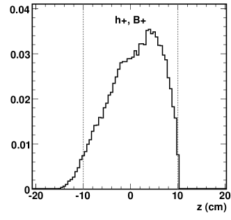
(a) h$+$, B$+$

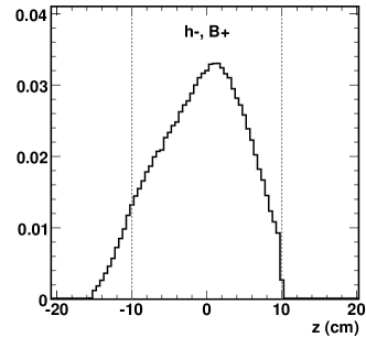
(b) h$-$, B$+$

(c) h$-$, B$-$

(d) h$+$, B$-$

Figure 1: The longitudinal track origin, as determined by the track reconstruction, for each combination of electric charge and magnet polarity (see Sect. 2. 1(a) Positive hadrons, positive magnetic field. 1(b) Negative hadrons, positive magnetic field. 1(c) Negative hadrons, negative magnetic field. 1(d) Positive hadrons, negative magnetic field.

To reduce the number of events that were unlikely to produce particles in the Spectrometer acceptance, a vertex cut was imposed. As shown in Fig. 1, relatively few particles that originated further than 10 ${\rm cm}$ from the IP could be reconstructed. While some charged particles having a longitudinal origin 10 to 15 ${\rm cm}$ from the IP in the Au-direction could be reconstructed, the Spectrometer had a complicated acceptance in that region (as a function of transverse momentum). Because of this, only collisions that occurred within 10 ${\rm cm}$ of $z=0$, as determined by the OctDe vertexing algorithm, were used in the analysis. T0 information was used to reject events for which the OctDe vertexing algorithm yielded an unreasonable vertex. The “OctDeT0” condition required that the OctDe vertex agree with the T0 vertex to better than 25 ${\rm cm}$. This cut also served to further reduce background collisions between discordant bunches in which the T0 timing appeared good, but a corresponding collision vertex could not be found.

MC Selection

Variable	Condition	Summary
OctDe Vertex ($v_{z}$)	$-10~{}{\mbox{${\rm cm}$}}<v_{z}<+10~{}{\mbox{${\rm cm}$}}$	Collision in Spectrometer acceptance
d-side Paddle	Hit	One or more signals on d-side Paddle
Au-side Paddle	Hit	One or more signals on Au-side Paddle
d-side T0	Hit	One or more signals on d-side T0
Au-side T0	Hit	One or more signals on Au-side T0

Table 4: dAuSpectra event selection for d+Au MC.

The conditions required by the dAuSpectra event selection on simulated d+Au collisions are shown in Table 4. The OctDe vertex requirement was kept the same for MC as for data, as were the requirements that both Paddle and T0 detectors be hit. However, due to the lack of timing information in the simulations, no timing cuts were applied to the T0s.

2 Track Selection

Once an event had passed the event selection, certain cuts were imposed on the reconstructed particles. The curved tracking itself took steps to remove duplicate tracks and to discard tracks that had large residuals, as discussed in Ch. 4. However, further steps were taken to remove particle tracks that were not reliably reconstructed.

1 Fit Probability Cut

First, tracks with poor momentum fits were removed. This was done by making a cut on the fit probability, calculated from the $\chi^{2}$ statistic described in Sect. 2. Given the $\chi^{2}$ value of the track, $\chi^{2}_{t}$, and the number of hits on the track, $N_{h}$, the fit probability was calculated as

$$P\left(\frac{N_{h}}{2},\frac{\chi^{2}_{t}}{2}\right)=\frac{1}{\Gamma\left(\frac{N_{h}}{2}\right)}{\int_{{\chi^{2}_{t}}/2}^{+\infty}}e^{-t}t^{(N_{h}/2)-1}\mathit{dt}$$ (8)

where $P$ represents the probability that, given the same physical particle, the tracking procedure would yield a worse fit purely by chance. The probability is normalized by the so-called Gamma function,

$$\Gamma\left(\frac{N_{h}}{2}\right)=\int_{0}^{+\infty}e^{-u}u^{(N_{h}/2)-1}\mathit{du}$$ (9)

The distribution of fit probabilities obtained for all the tracks was expected to be flat. To see this, suppose one performed measurements of a set of random variables $y_{i}$. Suppose further that each individual measurement was a sampling of a Gaussian distribution with mean $\mu_{i}$ (thus the expected value) and standard deviation $\sigma_{i}$ (thus the measurement error). Then the sum

$$\chi^{2}=\sum_{i=1}^{N}\left(\frac{y_{i}-\mu_{i}}{\sigma_{i}}\right)^{2}$$ (10)

would follow a $\chi^{2}$ distribution (by definition), with $k=N-\nu$ degrees of freedom, where $\nu$ is the number of parameters used to determine each $\mu_{i}$. For example, the $\chi^{2}$ of a track could be calculated by taking each $y_{i}$ to be the position of a hit on the track, each $\mu_{i}$ to be the expected hit position and each $\sigma_{i}$ to be the relevant measurement error. Then the values obtained by calculating the sum in Eq. 10 for each track would be distributed according to a $\chi^{2}$ distribution. The $\chi^{2}$ distribution is shown in Fig. 2(a) (for $k=4$) and is defined by

$$\mathscr{P}\left(\chi^{2}\right)=\frac{(1/2)^{k/2}}{\Gamma(k/2)}{\left(\chi^{2}\right)}^{k/2-1}e^{-\chi^{2}/2}$$ (11)

(a) $\chi^{2}$ Distribution

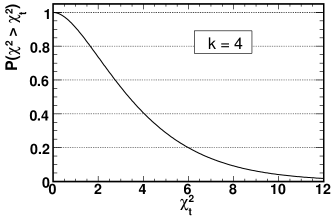
(b) $\chi^{2}$ Probability

Figure 2: 2(a) The $\chi^{2}$ (probability density) distribution with four degrees of freedom. See text for an explanation of the shaded regions. 2(b) The corresponding $\chi^{2}$ complementary cumulative distribution function, which gives the probability that an observed $\chi^{2}$ could be greater than some $\chi^{2}_{t}$ purely by chance.

The probability calculated by Eq. 8 is simply the integral of this function over values above the measured $\chi^{2}_{t}$, and is shown in Fig. 2(b) for $k=4$. The vertical lines in Fig. 2(a) show the $\chi^{2}$ values corresponding to 90% fit probability $\left(\chi^{2}=1.06\right)$, 80% probability $\left(\chi^{2}=1.64\right)$, and so on. Notice that the area of the shaded regions between these lines are all equal – as they have to be, since they all represent a 10% wide probability “bin.” Thus, any measured $\chi^{2}_{t}$ value is equally likely to fall into any one of the 10% wide probability bins.

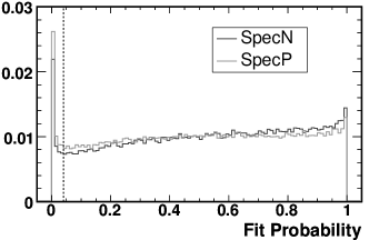
(a) Fit Probability Cut

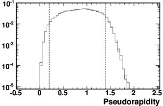
(b) Pseudorapidity Cut

Figure 3: Cuts made to select tracks for the analysis. Black dashed lines show the cuts, solid dark grey lines show the distribution for SpecN and solid light grey lines show the distribution for SpecP. 3(a) Tracks with fit probability below 4% were not used in the analysis. 3(b) Tracks outside the Spectrometer’s acceptance, $0.2<\eta<1.4$, were cut.

It follows that, if the values of $\chi^{2}_{t}$ calculated for each reconstructed particle track were actually distributed according to Eq. 11, then the distribution of fit probabilities seen in the data would be flat. Any deviation from flatness would indicate that the errors were not properly calculated. As seen in Fig. 3(a), there was an excess of tracks with a fit probability below 4%. It was inferred that the errors used for these tracks (taken from the covariance matrices) did not properly describe the deviation of hits from the reconstructed particle trajectory. Thus, it was unlikely that the reconstructed track actually described a physical particle that produced the observed distribution of hits. Therefore, these tracks were not used in the analysis.

2 Spectrometer Acceptance Cut

The next track quality cut ensured that only tracks that were within the pseudorapidity acceptance of the Spectrometer were used. This cut was performed mainly to simplify the pseudorapidity normalization (the “$\mathit{d\eta}$” in Eq. 5). The pseudorapidity distribution of tracks in the d+Au data is shown in Fig. 3(b). Note that the distribution drops rapidly outside of the cuts. Only tracks with a pseudorapidity value between 0.2 and 1.4 units were used in the analysis.

3 Distance to Beam Cut

Finally, a cut was implemented to remove particles known as secondaries. That is, particles that were not directly produced by the d+Au collision. For a Au+Au collision, this would have been done by requiring that a reconstructed particle be produced a short distance from the collision vertex. However, because the vertexing resolution in d+Au was roughly two orders of magnitude larger (in the beam direction), a different procedure was used for the d+Au analysis.

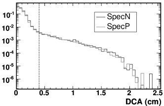
(a) DCA Cut

Figure 4: Tracks that did not originate within 4 ${\rm mm}$ of the beam orbit were cut. 4(a) The $\mathit{DCA}_{\rm beam}$ distribution observed in the +̣Au data. 4(b) The $\mathit{DCA}_{\rm beam}$ distribution seen in the HIJING simulations. 4(c) The fraction of primaries in the HIJING simulations that would be rejected by cutting at a given $\mathit{DCA}_{\rm beam}$.

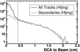
(b) HIJING DCA

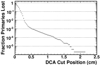
(c) Rejected Primaries (HIJING)

In this procedure, the trajectory of the particle was extrapolated back to the beam line, using the particle’s initial momentum vector. Then, the distance of closest approach, $\mathit{DCA}_{\rm beam}$, between the three-dimensional line of the particle’s trajectory and the the three-dimensional line of the beam orbit was calculated. The distribution of this distance for tracks in the d+Au data is shown in Fig. 4(a). The peak below distances of 4 ${\rm mm}$ was due mainly to primary particles (those produced directly by the d+Au collision), while the tail of the distribution was due to secondaries. This could be seen easily in HIJING simulations, as shown in Fig. 4(b). Thus, only particles that came within 4 ${\rm mm}$ of the beam orbit were used in the analysis. This cut rejected less than 0.2% of all primaries, as can be seen in Fig. 4(c), which shows the fraction of primaries rejected as a function of the $\mathit{DCA}_{\rm beam}$ cut. The accuracy with which the HIJING simulations reproduced the track distributions seen in the d+Au data is discussed in Sect. 2.

3 Measuring Hadron Spectra

With an ideal experiment, it would be possible to observe every collision, no matter how peripheral, and to measure every particle produced by the collision, with no contribution from any background (such as secondaries). In that case, measuring the transverse momentum spectra of hadrons would be easy. The experimenter would simply count the number of charged hadrons observed in bins of $p_{\mathrm{T}}$ and pseudorapidity, weighting each particle by $(2\pi p_{\mathrm{T}})^{-1}$. Each bin would then be divided by the number of collisions, and normalized by the bin widths.

In a real experiment, it is not possible to obtain such a direct measurement of the charged hadron spectra. While the fundamental procedure for finding the spectra remains the same, various corrections are needed to account for experimental effects that cause the number of observed charged particles to differ from the number of produced charged particles. These corrections were determined by estimating the effects of experimental imperfections using simulations.

1 Acceptance and Efficiency

Charge	Polarity	Bending Direction
$\rm{h}^{+}$	B$+$	Toward the beam line
$\rm{h}^{+}$	B$-$	Away from the beam line
$\rm{h}^{-}$	B$+$	Away from the beam line
$\rm{h}^{-}$	B$-$	Toward the beam line

Table 5: Definition of the bending direction of a charged hadron in the PHOBOS magnetic field.

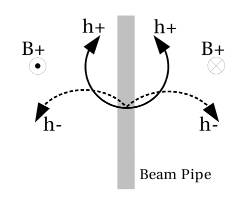
Figure 5: The bending direction of positive (solid arrow) and negative (dashed arrow) hadrons in a positively oriented magnetic field.

The largest correction made to the spectra accounted for the limited acceptance of the PHOBOS Spectrometer and for the efficiency of the tracking procedure. The correction depended on the transverse momentum of the particle, the electric charge of the particle, the longitudinal collision position, the polarity of the magnetic field and on the Spectrometer arm used to reconstruct the particle. The dependence on charge and magnetic field were related, however. A positively charged pion with momentum $p$ traveling through a magnetic field of positive polarity (B$+$) follows the same trajectory as a negatively charged pion with momentum $p$ traveling through a magnetic field with opposite (B$-$) polarity. Thus, the correction depended on the so-called bending direction of the particle, described in Table 5, rather than on the four combinations of charge and polarity. Note that a magnetic field of one polarity, say B$+$, would be oriented up-wards on one side of the beam line and down-wards on the other. The result was that particles of the same charge would bend in the same direction, either away from or toward the beam line, no matter which Spectrometer arm they traveled through, as shown in Fig. 5.

Parameter	Minimum	Maximum
$z_{0}$	$-$10 ${\rm cm}$	$+$10 ${\rm cm}$
$p_{\mathrm{T}}$	0.15 GeV$\kern-1.49994pt/\kern-1.19995ptc$	7.0 GeV$\kern-1.49994pt/\kern-1.19995ptc$
$y$	0	1.5
$\phi$	$-$0.2 ${\rm rad}$	$+$0.2 ${\rm rad}$

Table 6: The physical parameters used to simulate pions for the Spectrometer acceptance and tracking efficiency corrections.

The size of the correction was determined by simulating the response of the Spectrometer and tracking procedure to individual particles. Ten million charged pions were simulated and separately reconstructed in each of the eight combinations of: $\pi^{+}$ or $\pi^{-}$, B$+$ or B$-$, and reconstruction in the inner-ring Spectrometer arm (SpecN) or the outer-ring Spectrometer arm (SpecP). The simulated pions were generated using four parameters to describe the particle’s trajectory: longitudinal origin, $z_{0}$, transverse momentum, $p_{\mathrm{T}}$, rapidity, $y$, and azimuthal angle, $\phi$. For each particle, random values of these parameters were chosen between the limits shown in Table 6. To account for the collision position dependence, the corrections were determined in four bins of $z_{0}$, each 5 ${\rm cm}$ wide. Particles were simulated over a range of azimuthal angle that was sufficient to cover the acceptance of one Spectrometer arm, but was smaller than $\pi$. Therefore, an extra factor of $\pi/(0.4~{}\mbox{${\rm rad}$})\approx 7.85$ was required to correct the measured spectra up to the azimuthally averaged yield described in Eq. 5.

The simulation of each particle generated “hits” in the Spectrometer. This allowed the tracking procedure to be run on a simulated event containing only one particle. The tracking would then either fail to find any track, or it would produce a single reconstructed particle track. Very rarely, multiple tracks would be found; these events were explicitly discarded, as this effect of the tracking was taken into account by the ghost correction discussed in Sect. 2.

To find the correction, the number of particles simulated was recorded in bins of $p_{\mathrm{T}}$, $z_{0}$, Spectrometer arm and bending direction. Only particles with $0.2<\eta<1.4$ were used to find the correction (to correspond with the pseudorapidity range used in the analysis). Then the number of successfully reconstructed tracks in each bin was recorded. A track was successfully reconstructed if (a) the tracking procedure produced a track and (b) the reconstructed particle passed the track selection cuts described in Sect. 2. Note that only the true simulation parameters of a particle were used to choose in which bin the track should be counted. For example, suppose two $p_{\mathrm{T}}$ bins were used, where bin $A$ counted tracks with $p_{\mathrm{T}}<1~{}\mbox{\rm GeV$\kern-1.49994pt/\kern-1.19995ptc$}$ and bin $B$ counted tracks with $p_{\mathrm{T}}>1~{}\mbox{\rm GeV$\kern-1.49994pt/\kern-1.19995ptc$}$. If a particle was simulated with $p_{\mathrm{T}}=0.9~{}\mbox{\rm GeV$\kern-1.49994pt/\kern-1.19995ptc$}$ but reconstructed as having $p_{\mathrm{T}}=1.1~{}\mbox{\rm GeV$\kern-1.49994pt/\kern-1.19995ptc$}$, then both the number of simulated and the number of reconstructed particles in bin $A$ would be increased. This was done so that the momentum resolution of the tracking (see Sect. 7) could be accounted for separately from the efficiency of the tracking. The true value of $z_{0}$ was also used, to prevent vertexing efficiency from entering into this correction.

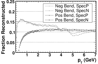
(a) $-10~{}\mbox{${\rm cm}$}<z_{0}<-5~{}\mbox{${\rm cm}$}$

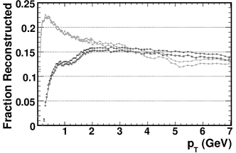
(b) $-5~{}\mbox{${\rm cm}$}<z_{0}<0~{}\mbox{${\rm cm}$}$

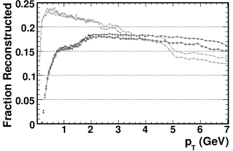
(c) $0~{}\mbox{${\rm cm}$}<z_{0}<+5~{}\mbox{${\rm cm}$}$

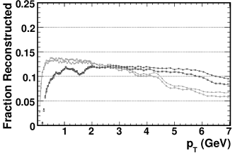
(d) $+5~{}\mbox{${\rm cm}$}<z_{0}<+10~{}\mbox{${\rm cm}$}$

Figure 6: The Spectrometer acceptance and tracking efficiency corrections as determined by the fraction of successfully reconstructed pions in bins of $p_{\mathrm{T}}$, track origin ($z_{0}$), Spectrometer arm and bending direction.

		Minimum $p_{\mathrm{T}}$ (GeV$\kern-1.49994pt/\kern-1.19995ptc$)
Bending Dir.	Spec. Arm	$z_{0}=(-10~{}\mbox{${\rm cm}$},~{}-5~{}\mbox{${\rm cm}$})$	$(-5,~{}0)$	$(0,~{}5)$	$(5,~{}10)$
Toward	SpecP	0.39	0.29	0.29	0.29
Toward	SpecN	0.39	0.29	0.29	0.29
Away	SpecP	0.09	0.09	0.09	0.09
Away	SpecN	0.09	0.09	0.09	0.09

Table 7: The minimum $p_{\mathrm{T}}$ used to measure particles in each track origin, Spectrometer arm and bending direction bin.

The value of the correction in a bin was the fraction of simulated particles that were successfully reconstructed. The corrections were stored as histograms, with separate histograms for each combination of track origin bin, Spectrometer arm and bending direction. Each histogram contained bins of $p_{\mathrm{T}}$, with $0.05~{}\mbox{\rm GeV$\kern-1.49994pt/\kern-1.19995ptc$}$ wide bins up to $2~{}\mbox{\rm GeV$\kern-1.49994pt/\kern-1.19995ptc$}$, $0.1~{}\mbox{\rm GeV$\kern-1.49994pt/\kern-1.19995ptc$}$ wide bins up to $4~{}\mbox{\rm GeV$\kern-1.49994pt/\kern-1.19995ptc$}$ and $0.15~{}\mbox{\rm GeV$\kern-1.49994pt/\kern-1.19995ptc$}$ wide bins above $4~{}\mbox{\rm GeV$\kern-1.49994pt/\kern-1.19995ptc$}$. The histograms were then fit with $3^{rd}$ degree polynomial splines. The fits allowed interpolation between the $p_{\mathrm{T}}$ bin centers and were used to estimate the corrections for particles having any transverse momentum up to $7~{}\mbox{\rm GeV$\kern-1.49994pt/\kern-1.19995ptc$}$. The minimum $p_{\mathrm{T}}$ used to fit each spline was not the lowest point in the histogram. Instead, a minimum was chosen to correspond to the point at which the tracking efficiency dropped to roughly 30% of the maximum. This was done to avoid systematic errors resulting from (a) interpolating between points in a rapidly changing function and (b) measuring particles in a region of $p_{\mathrm{T}}$ where the efficiency may not be well determined. The minimum $p_{\mathrm{T}}$ values used in the spline fits, and therefore also the minimum $p_{\mathrm{T}}$ used in the spectra measurements, are show in Table 7. The resulting corrections are shown in Fig. 6.

2 Ghost and Secondary Particles

While the efficiency of the tracking procedure could be understood by simulating single particles, further studies were necessary to estimate how often a successfully reconstructed track was not actually a measurement of a primary particle. Such tracks introduced errors on the number of primary particles per d+Au collision counted by the analysis. These errors were corrected for by investigating two sources of such mis-identified tracks. One source was reconstructed tracks that did not actually correspond to any physical particle, but were constructed out of hits from different particles (or detector noise). These tracks were known as ghosts. The other source was successfully reconstructed secondaries.

Full d+Au collision simulations were used to estimate the number of ghosts and secondaries that would be observed in the data. This was done by first running the tracking procedure on each simulated event. The reconstructed tracks were then matched to the underlying simulated particles by finding shared hits. That is, for a given Silicon pad that was hit by a reconstructed track, all simulated particles that deposited energy into the same pad were said to share a hit with the track. The simulated particle that shared the most hits with a reconstructed track was the best match for that track.

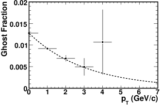
(a) Ghosts

(b) Secondaries

Figure 7: Ghost and secondary tracks. The dashed black lines show the fits used in the analysis. 7(a) The fraction of successfully reconstructed tracks due to ghosts. 7(b) The fraction of successfully reconstructed tracks due to secondaries.

Tracks due to secondaries and ghosts were then easy to identify. Secondary tracks were successfully reconstructed tracks (i.e. those that passed the track selection described in Sect. 2) whose best matching simulated particle was not a primary. Ghost tracks were successfully reconstructed tracks that did not share ten or more hits with any simulated particle. The ghost (secondary) correction was then simply the ratio of the number of reconstructed ghost (secondary) tracks to the total number of successfully reconstructed tracks, in bins of reconstructed transverse momentum. The corrections were originally calculated in each centrality bin, however it was found that neither the secondary nor the ghost correction depended on centrality. Figure 7 shows the fractions of ghost and secondary tracks expected to be present in the data.

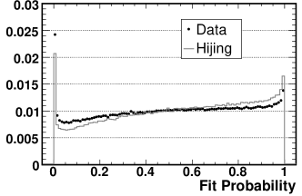
(a) Fit Probability

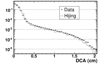
(b) DCA Beam

Figure 8: Comparison of reconstructed track distributions from HIJING (grey line) and d+Au data (black points). 8(a) The fit probability distributions. 8(b) The distance of closest approach to the beam orbit distributions.

Collisions	Tracks with Fit Prob. $<$ 4%
d+Au Data	4.96%
AMPT	4.08%
Hijing	4.14%

Table 8: The fraction of tracks rejected by the fit probability cut.

Since these corrections relied on MC simulations, it was necessary to ensure that the simulations provided a reasonably accurate description of reality. The $\mathit{DCA}_{\rm beam}$ and the fit probability distributions from HIJING simulations are compared to the distributions from the d+Au data in Fig. 8. The corresponding distributions from AMPT were nearly identical. This allowed the results of both AMPT and HIJING simulations to be combined to find the ghost and secondary track corrections with better statistics. While the fit probability distributions differed slightly between data and simulation, the fraction of tracks rejected by the fit probability cut was essentially the same in the data as it was in the simulations, as shown in Table 8. Thus, the simulations provided an accurate description of the observed tracking behavior and detector response.

3 Dead and Hot Spectrometer Pads

Silicon channels that did not function properly introduced another source of error into the analysis. There were two types of problematic channels: those that reported a signal without being hit (a hot channel) and those that reported no signal when hit (a dead channel). Hot channels were identified as those that reported either many more hits than the average channel and/or much more energy per hit than the average channel. Dead channels were identified as those that reported many fewer hits than the average channel and/or much less energy per hit than the average channel.

During the d+Au spectra analysis, signals from hot and dead channels were used when reconstructing tracks. The effects of including these channels was studied using both d+Au data and MC simulations. It was assumed that hot channels would increase the number of ghost tracks in the data, since the tracking could (wrongly) associate a false hit on a hot channel with a track. On the other hand, dead channels were assumed to decrease the number of tracks that could be reconstructed, since hits from particles passing through these channels could not be observed.

	Data	Single Particle Simulation
Spectrometer Arm	Masked / Unmasked	Masked / Unmasked	Correction
SpecP	0.8410	0.8157	1.031
SpecN	0.7640	0.6840	1.117

Table 9: The hot and dead channel correction.

To estimate the effect of hot channels, one million d+Au collisions were reprocessed with hot and dead channels masked out. That is, hits on those channels were not used to reconstruct tracks. This reduced the number of tracks that were successfully reconstructed in these collisions by about 16% in SpecP and 24% in SpecN, as shown in Table 9. The magnitude of this difference quantified the relative number of ghost tracks created by hot channels. Note that these ghost tracks were not accounted for in the correction described in Sect. 2 since there were no hot channels in the simulations.

The reduced efficiency of the tracking due to dead channels was estimated using single-track simulations, similar to those described in Sect. 1. One million single tracks were simulated in each combination of $\pi^{+}$ or $\pi^{-}$, B$+$ or B$-$, and reconstruction in SpecN or SpecP. For these simulations, track reconstruction was run with the hot and dead channels masked out. This reduced the single track reconstruction efficiency, as compared to the efficiency described in Sect. 1, by about 18% in SpecP and 32% in SpecN, as shown in Table 9. The reason masked out channels had such a significant impact on the tracking efficiency was due to the large number of hits required on a track, as discussed in Ch. 4.

Spectrometer Arm	Hot Channels	Dead Channels
SpecP	0.98%	2.07%
SpecN	1.39%	3.55%

Table 10: The fraction of hot and dead channels in each Spectrometer arm.

The final correction to the number of tracks observed in the data without masking hot or dead channels was then

$$C_{HD}=\left(\frac{\text{Data Masked}}{\text{Data Unmasked}}\right)\bigg{/}\left(\frac{\text{Single Track Masked}}{\text{Single Track Unmasked}}\right)$$ (12)

where $C_{HD}$ is the value of the hot and dead channel correction for a Spectrometer arm. The first term of Eq. 12 reduces the number reconstructed tracks by the fraction of ghosts expected to originate from hot channels. The second term reduces the efficiency of the tracking that was estimated in simulations of a Spectrometer with no dead channels. It accounts for the reduced number of Spectrometer pads available due to dead channels. Since the raw number of tracks will be divided by the tracking efficiency (see Eq. 14), this term is in the denominator.

The values used in this analysis to correct for hot and dead channels are shown in Table 9. The fraction of hot and dead channels in each Spectrometer arm was not large, as can be seen in Table 10. However, the correction for SpecN was much larger than the correction for SpecP. This was due mainly to the fact that three out of the four sensors on the fifth plane of SpecN had many problematic channels.

4 Event Selection Efficiency

As discussed in Sect. 1, the efficiency of the detector to observe collisions that satisfy the chosen event selection was estimated using MC simulations. This efficiency estimate can be used to correct the observed hadron spectra, in order to measure the number of charged particles produced per collision, rather than the number of charged particles per observed collision. These quantities would be equal if the efficiency of measuring a collision did not depend on the properties of that collision. For example, suppose one could detect half of all collisions, irrespective of the properties of those collisions. In that case, on average one would also detect half of the tracks produced by all the collisions that actually occurred. Then the ratio of the number of tracks observed to the number of collisions observed is of course the same as ratio of the number of tracks actually produced to the number of collisions that actually occurred. However, as seen in Sect. 1, the efficiency of measuring a collision did in fact depend on the centrality of that collision.

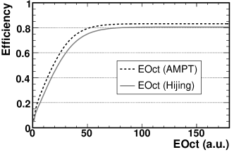
(a) EOct Efficiency

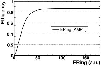
(b) ERing Efficiency

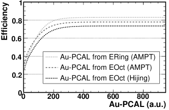
(c) Au-PCAL Efficiency

Figure 9: The dAuSpectra event selection efficiency as a function of the different centrality measures.

The centrality dependence of the event selection efficiency could be accounted for in different ways. First, a model (i.e. Glauber) could be used to parametrize the bias introduced by the varying efficiency. This would be done by (a) applying the event selection to a group of simulated collisions, (b) using a model to calculate a centrality parameter like $N_{\rm part}$ for each selected collision and then (c) finding the average of the centrality parameter for that group of collisions. This procedure would give, for example, a biased number of participants ($N_{\rm part}^{\rm biased}$) for each centrality bin. For the efficiency shown in Fig. 9(b), $N_{\rm part}^{\rm biased}$ of the most central bin would be equal to $N_{\rm part}$ in that bin, since the efficiency is flat in the central bin. However, $N_{\rm part}^{\rm biased}$ of the most peripheral bin would be significantly larger than the average number of participants for all collisions in the peripheral bin. In this way, the measured spectra would be the number of charged hadrons produced by collisions having an average number of participants equal to $N_{\rm part}^{\rm biased}$.

In this analysis, a different procedure was used; namely, the estimated efficiency was used to correct the spectra. This provided a measurement of the average number of particles produced by collisions in a certain fractional cross section bin. Applying this correction was straight-forward. For any given collision, the efficiency was determined using the chosen centrality measure (i.e. EOct). Then, both the number of tracks and the number of collisions were weighted by this efficiency. For example, if collision $A$ had an efficiency of 100% and one track was observed, then the total number of tracks and collisions would be increased by one. Whereas if collision $B$ had an efficiency of only 50% and two tracks were observed, then the total number of tracks would be increased by four and the total number of collisions would be increased by two. The dAuSpectra event selection efficiency corrections for each centrality measure used in the analysis is shown in Fig. 9.

5 Event Normalization

Taking all the corrections into account, the average charged hadron yield per collision, $\left<Y\right>$, in a particular bin (of $p_{\mathrm{T}}$, fractional cross section and electric charge) was simply the total corrected number of tracks in that bin, $t_{\rm tot}$, divided by the total corrected number of events in that bin, $n_{\rm tot}$,

$$\left<Y(p_{\mathrm{T}},~{}\text{crs.~{}scn.},~{}\text{charge})\right>=\frac{t_{\rm tot}}{n_{\rm tot}}=\frac{\sum^{N}_{e=1}\left(\frac{1}{\epsilon_{e}}\sum^{T_{e}}_{i=1}\left(w_{i}\right)\right)}{\sum^{N}_{e=1}\left(\frac{1}{\epsilon_{e}}\right)}$$ (13)

where $\epsilon_{e}$ is the event selection efficiency for the collision, $w_{i}$ is the weight given to each track by the corrections, $N$ is the (uncorrected) number of measured collisions and $T_{e}$ is the (uncorrected) number of reconstructed tracks in the event. The full track weighting was calculated by

$$w=\frac{\left(1-G(p_{\mathrm{T}})\right)~{}\left(1-S(p_{\mathrm{T}})\right)~{}C_{HD}(\text{arm})~{}\left(7.85/A(p_{\mathrm{T}},z_{0},\text{arm},\text{bend})\right)}{2\pi p_{\mathrm{T}}~{}\Delta\eta}$$ (14)

where $p_{\mathrm{T}}$ is the transverse momentum of the particle, $z_{0}$ is the longitudinal collision vertex, ‘arm’ is the Spectrometer arm in which the track was reconstructed, ‘bend’ is the bending direction of the track, $G$ is the fraction of ghost tracks, $S$ is the fraction of secondaries, $C_{HD}$ is the hot and dead channel correction, $A$ is the acceptance and efficiency correction and $\Delta\eta=1.2~{}{\rm units}$ is the range of pseudorapidity over which particles were counted.

The event normalization was complicated, however, by the dependence of the acceptance on bending direction and collision vertex, shown in Table 7. For example, a positive hadron having $p_{\mathrm{T}}=250~{}\mbox{\rm MeV$\kern-1.49994pt/\kern-1.19995ptc$}$ could be measured with the PHOBOS magnet in negative polarity, but not with the magnet in the positive polarity. During the analysis, the number of particles were counted separately for each combination of charge, magnet polarity and spectrometer arm. This was necessary both to apply the acceptance and efficiency corrections (see Sect. 1) and to allow the separate charged spectra to be measured. The number of collisions observed was counted separately for each magnet polarity.

It was then necessary to properly sum the corrected number of tracks in a given $p_{\mathrm{T}}$ bin and to sum the corresponding corrected number of events. However, the example above suggests that in certain ranges of $p_{\mathrm{T}}$, only collisions from one magnet polarity should be counted when measuring particles of a particular charge. Therefore, the number of collisions used to normalize a particular hadron spectra was dependent on $p_{\mathrm{T}}$.

Collision Num.	Magnet Polarity	$p_{\mathrm{T}}$ (GeV$\kern-1.49994pt/\kern-1.19995ptc$)	Observed?
1	B$-$	0.21	Yes
2	B$+$	0.25	No
3	B$-$	0.42	Yes
4	B$+$	0.35	Yes
5	B$-$	0.55	Yes

Table 11: Measurements made by the simple example detector described in the text.

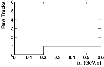
(a) Raw Tracks

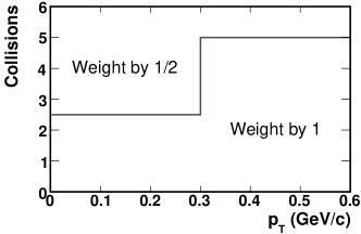
(b) Summed Collisions

Figure 10: A simple example of the event normalization procedure for a detector which measures particles having $p_{\mathrm{T}}<0.3~{}\mbox{\rm GeV$\kern-1.49994pt/\kern-1.19995ptc$}$ in only one of two possible magnet polarities.

A very simple example can illustrate this subtle point. Imagine a nearly perfect detector that has 100% efficiency inside its acceptance, but can not observe particles below $p_{\mathrm{T}}=0.3~{}\mbox{\rm GeV$\kern-1.49994pt/\kern-1.19995ptc$}$ when its magnet polarity is positive. This detector is then used to measure the yield of hadrons from five interactions. These raw measurements are shown in Table 11. Thus, the raw $p_{\mathrm{T}}$ spectrum of these collisions is presented in Fig. 10(a) for $p_{\mathrm{T}}$ bins of 0.1 GeV$\kern-1.49994pt/\kern-1.19995ptc$. It is clear from Table 11 that the final yield of positive hadrons should be 2/5 in the $0.2\to 0.3$ bin, and 1/5 in the higher bins. However, this result is not obtained by simply dividing the raw $p_{\mathrm{T}}$ spectrum shown in Fig. 10(a) by the number of collisions (5). The reason is that for $p_{\mathrm{T}}<0.3~{}\mbox{\rm GeV$\kern-1.49994pt/\kern-1.19995ptc$}$, only one of the two possible magnet polarities will allow a particle to be detected. Thus, when normalizing the raw spectrum for $p_{\mathrm{T}}<0.3~{}\mbox{\rm GeV$\kern-1.49994pt/\kern-1.19995ptc$}$, the number of collisions should be weighted by one half, as shown in Fig. 10(b). Dividing the raw $p_{\mathrm{T}}$ spectrum shown in Fig. 10(a) by the number of collisions versus $p_{\mathrm{T}}$ shown in Fig. 10(b) then produces the correct yield. While this is a simple example, an analogous procedure was used to normalize the hadron yields measured in this thesis.

6 Statistical Errors

To find the statistical error of the average yield given by Eq. 13, it was necessary to treat each measured collision as a sampling of two random (but correlated) variables: the corrected number of tracks per event, $t$, and the corrected number of collisions per event, $n$. Note that the average of $t/n$ is equal to $t_{\rm tot}/n_{\rm tot}$. The error on the mean of the ratio $t/n$ in bin $B$ was then calculated in the usual way,

$$\sigma\left(\left<Y_{B}\right>\right)=\frac{\left<Y_{B}\right>}{\sqrt{N}}\sqrt{\frac{\sigma^{2}_{t}}{\left<t\right>^{2}}+\frac{\sigma^{2}_{n}}{\left<n\right>^{2}}-2\frac{\mathrm{cov}(t,n)}{\left<t\right>\left<n\right>}}$$ (15)

where $N$ is the (uncorrected) number of measured collisions. The mean and standard deviation of $n$ and $t$ were calculated by

$$\left<n\right> =\frac{1}{N}\sum_{e=1}^{N}\left(n_{e}\right) \sigma^{2}_{n} =\frac{1}{N}\sum_{e=1}^{N}\left(n_{e}-\left<n\right>\right)^{2} n_{e} =\frac{1}{\epsilon_{e}}$$ where (16)

$$\left<t\right> =\frac{1}{N}\sum_{e=1}^{N}\left(t_{e}\right) \sigma^{2}_{t} =\frac{1}{N}\sum_{e=1}^{N}\left(t_{e}-\left<t\right>\right)^{2} t_{e} =\frac{1}{\epsilon_{e}}\sum^{T_{e}}_{j=1}\left(\frac{1}{w_{j}}\right)$$ where (17)

The covariance was calculated by

$$\mathrm{cov}(t,n)=\frac{1}{N}\sum_{e=1}^{N}\left(n_{e}-\left<n\right>\right)\left(t_{e}-\left<t\right>\right)$$ (18)

Calculation of these variances was simplified by exploiting the fact that

$$\sigma^{2}_{x} =\frac{1}{N}\sum_{e=1}^{N}\left(x_{e}-\left<x\right>\right)^{2}=\frac{1}{N}\sum_{e=1}^{N}\left(x_{e}^{2}-2x_{e}\left<x\right>+\left<x\right>^{2}\right)$$

$$=\frac{1}{N}\sum_{e=1}^{N}\left(x_{e}^{2}\right)-2\left<x\right>\left(\frac{1}{N}\sum_{e=1}^{N}x_{e}\right)+\left<x\right>^{2}=\left<\smash[t]{x^{2}}\right>-2\left<x\right>^{2}+\left<x\right>^{2}$$

$$\sigma^{2}_{x} =\left<\smash[t]{x^{2}}\right>-\left<x\right>^{2}$$ (19)

and

$$\mathrm{cov}(t,n) =\frac{1}{N}\sum_{e=1}^{N}\left(n_{e}-\left<n\right>\right)\left(t_{e}-\left<t\right>\right)=\frac{1}{N}\sum_{e=1}^{N}\left(n_{e}t_{e}-t_{e}\left<n\right>-\left<t\right>n_{e}+\left<t\right>\left<n\right>\right)$$

$$=\left<nt\right>-\left<n\right>\frac{1}{N}\sum_{e=1}^{N}\left(t_{e}\right)-\left<t\right>\frac{1}{N}\sum_{e=1}^{N}\left(n_{e}\right)+\left<t\right>\left<n\right>$$

$$\mathrm{cov}(t,n) =\left<nt\right>-\left<n\right>\left<t\right>$$ (20)

where $x$ can be either $t$ or $n$. Equations 19 and 20 allowed the variances to be computed by summing different quantities in a single processing of the data. Without these identities, it would have been necessary to analyze the data once to calculate the mean values $\left<n\right>$ and $\left<t\right>$, and then to analyze the data a second time to calculate the standard deviations from these means.

Note that for the special case in which the event selection efficiency is constant and the number of particles produced follows a Poisson distribution, Eq. 15 reduces to the standard form $\sigma\left(\left<Y_{B}\right>\right)=\sqrt{\left<Y_{B}\right>/N}$. To see this, take $\epsilon_{e}\rightarrow 1$. Then

$$n_{e}=\frac{1}{\epsilon_{e}} =1 \sigma^{2}_{n} =0 \mathrm{cov}(t,n) =0$$

$$\left<n\right>=\frac{1}{N}\sum_{e=1}^{N}\left(n_{e}\right) =1 \left<Y_{B}\right> =\left<\frac{t}{n}\right>=\left<t\right> \sigma^{2}_{t} =\left<t\right>$$

so

$$\sigma\left(\left<Y_{B}\right>\right) =\frac{\left<Y_{B}\right>}{\sqrt{N}}\sqrt{\frac{\sigma^{2}_{t}}{\left<t\right>^{2}}+\frac{\sigma^{2}_{n}}{\left<n\right>^{2}}-2\frac{\mathrm{cov}(t,n)}{\left<t\right>\left<n\right>}}$$

$$=\frac{\left<Y_{B}\right>}{\sqrt{N}}\sqrt{\frac{\left<t\right>}{\left<t\right>^{2}}}=\sqrt{\frac{\left<Y_{B}\right>^{2}}{N\left<t\right>}}$$

$$\sigma\left(\left<Y_{B}\right>\right) =\sqrt{\frac{\left<Y_{B}\right>}{N}}\quad\text{for}\quad\epsilon_{e}=1$$

which is the error on the number of particles per collision in a particular bin, when each collision is weighted equally and when the number of particles per collision in the bin follows a Poisson distribution.

7 Momentum Resolution and Binning

Once the spectra had been produced, a final correction was necessary. This correction accounted for the momentum resolution of the tracking algorithm and for the varying $p_{\mathrm{T}}$ bin sizes. Because the invariant yield of charged hadrons followed a steeply falling curve, errors in the reconstructed momentum of a particle led to an excess of particles at higher $p_{\mathrm{T}}$. To see this, consider an example in which measurements are made of an extremely steeply falling slope. Suppose that the yield were measured in only two bins, with bin $A$ containing particles with $p_{\mathrm{T}}<1~{}\mbox{\rm GeV$\kern-1.49994pt/\kern-1.19995ptc$}$ and bin $B$ containing particles with $p_{\mathrm{T}}>1~{}\mbox{\rm GeV$\kern-1.49994pt/\kern-1.19995ptc$}$. Suppose further that after measuring 50 collisions, bin $A$ contained 400 particles, giving $Y_{A}=8$ and bin $B$ contained 10, giving $Y_{B}=0.2$. If an additional particle were produced with a transverse momentum of $0.9~{}\mbox{\rm GeV$\kern-1.49994pt/\kern-1.19995ptc$}$, then with an ideal detector, it would be counted in bin $A$, resulting in $Y_{A}=8.02$; a difference of only 0.25%. However, if the same particle were measured inaccurately as having $p_{\mathrm{T}}=1.1~{}\mbox{\rm GeV$\kern-1.49994pt/\kern-1.19995ptc$}$, then the particle would be counted in bin $B$, resulting in $Y_{B}=0.22$; a difference of 10%!

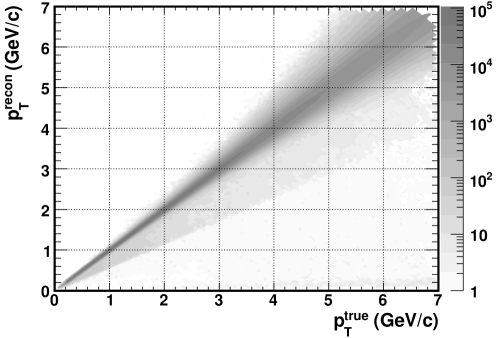
(a) Reconstructed Momentum

Figure 11: 11(a) The reconstructed transverse momentum of simulated pions as a function of the true $p_{\mathrm{T}}$ of the particle. 11(b) The reconstructed momentum distribution for particles having $p_{\mathrm{T}}\approx 1~{}\mbox{\rm GeV$\kern-1.49994pt/\kern-1.19995ptc$}$. 11(c) The reconstructed momentum distribution for particles having $p_{\mathrm{T}}\approx 3~{}\mbox{\rm GeV$\kern-1.49994pt/\kern-1.19995ptc$}$.

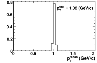
(b) $p_{\mathrm{T}}\approx 1~{}\mbox{\rm GeV$\kern-1.19995pt/\kern-0.95996ptc$}$

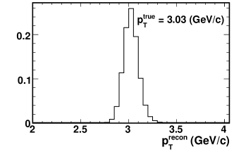
(c) $p_{\mathrm{T}}\approx 3~{}\mbox{\rm GeV$\kern-1.19995pt/\kern-0.95996ptc$}$

To correct for this effect, the momentum resolution of the tracking procedure was estimated using the single track simulations described in Sect. 1. From these simulations, the reconstructed momentum could be compared to the true momentum of the particle, as shown in Fig. 11(a). Note that the histogram in this figure was very finely binned, and that bins could be combined evenly to produce the same $p_{\mathrm{T}}$ binning as used in the spectra analysis.

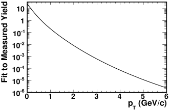
(a) Fit to Yield

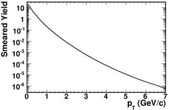
(b) Smeared Yield

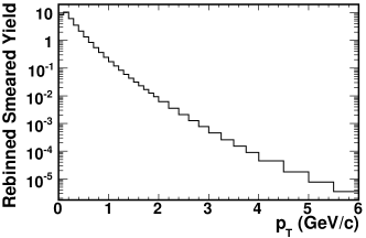
(c) Rebinned, Smeared Yield

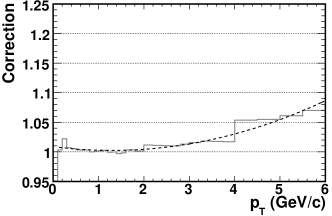
(d) Correction

Figure 12: Example of the steps necessary to determine the momentum resolution and binning correction. 12(a) A sample fit to some measured yield (data points not shown). 12(b) The smeared yield obtained by normalizing the momentum resolution to the measured yield. 12(c) The smeared yield rebinned to match the binning of the data. 12(d) The correction, obtained by dividing 12(c) by 12(a).

The correction was determined in several steps. First, the measured $p_{\mathrm{T}}$ spectra was fit with a smooth function, an example of which can be seen in Fig. 12(a). Next, the reconstructed $p_{\mathrm{T}}$ distribution in each $p_{\mathrm{T}}^{\text{true}}$ bin of Fig. 11(a) was independently normalized. The distribution in each $p_{\mathrm{T}}^{\text{true}}$ bin was then scaled up by the value of the yield at the center of the bin, as determined by the spectra fit. Next, this weighted two-dimensional histogram was projected onto the $p_{\mathrm{T}}^{\text{recon}}$ axis. This resulted in a hadron spectra distribution that was smeared by the momentum resolution, as seen in Fig. 12(b). Bins in this distribution were then combined in such a way as to recreate the same binning used in the analysis, as shown in Fig. 12(c). Finally, this smeared and re-binned distribution was then divided by the original fit to the spectra, as shown in Fig. 12(d). This histogram was then fit with a quadratic function to remove statistical fluctuations due to the number of tracks simulated. As can be seen in Fig. 12(d), this fit was smooth, and thus removed some of the correction that accounted for abrupt changes in bin size (note the jump at $p_{\mathrm{T}}=4~{}\mbox{\rm GeV$\kern-1.49994pt/\kern-1.19995ptc$}$). However, the discrepancy was less than 3%, and the systematic error on this correction was larger than that, as will be discussed in the next section.

8 Systematic Errors

Systematics of the Yield Measurements

Uncertainties in the precision of the spectra measurement originated from the number of observed collisions and particles, and were estimated by the statistical errors discussed in Sect. 6. Uncertainties in the accuracy of the measurement originated from the methods used to determine the various corrections. The largest such systematic uncertainty was associated with the largest correction: the acceptance and efficiency functions discussed in Sect. 1. To estimate this systematic error, the yield of d+Au collisions was reconstructed using several different subsets of the data. With perfect corrections, the yield measured in each subset of the data would be identical. Thus, the amount by which the yield varies from subset to subset gives an estimate of the systematic error associated with the correction.

For example, the yield of positive hadrons measured using only data taken with the PHOBOS magnet at positive polarity (B$+$) was compared to the same yield measured with B$-$ data. Since the bending direction of particles in these two measurements were different, the acceptance and efficiency corrections would be different. Therefore, variations in the positive hadron yield measured by these two subsets of the data could be associated with systematic uncertainties in the acceptance and efficiency correction. A host of such studies were done, and the resulting systematic error, similar to that used in [100], is shown in Fig. 13(a) as a function of $p_{\mathrm{T}}$.

The systematic uncertainty in the dead and hot channel correction was estimated in a similar way, by comparing the yields measured separately in each Spectrometer arm. In PHOBOS previous studies, discrepancies between the yield measured in each arm were not understood, see [100]. These effects have since been traced to a significant difference in the number of malfunctioning channels in the two arms, as discussed in Sect. 3. With the corrections applied separately to the two arms, discrepancies in the yields were reduced from $\sim 10\%$ to $\lesssim 3\%$. The systematic error shown in Fig. 13(d) represents both uncertainties associated with the correction and with the (small) differences in the yield measured separately with each Spectrometer arm.

For some corrections, such studies could not easily be performed. In each of these cases, the uncertainty was taken to be of the same magnitude as the correction itself. This was true for the momentum resolution and ghost corrections, see Fig. 13(b) and 13(e) respectively. For the secondary correction, the systematic error was larger than the correction at higher values of $p_{\mathrm{T}}$ to take into account the low statistics used to estimate the correction in this region, as shown in Fig. 13(c).

Finally, an uncertainty in the yield measured for nucleon-nucleus interactions was estimated. This was done by shifting the d-PCAL and d-ZDC energy cuts used to tag p+Au and n+Au collisions (see Sect. 4). If the minimum energy used to identify a proton or a neutron in one of the calorimeters was increased, it should affect only the number of interactions (and therefore particles) used to make the measurement. It should not have an impact on the yield. Thus, changing the tagging cut values provided an estimate of this additional systematic uncertainty in the yield of nucleon-nucleus interactions, and is presented in Fig. 13(f).

The total systematic error of the measured hadron yield was determined by taking the quadrature sum of the various contributions. Thus, the total systematic error on the yield of d+Au collisions, shown in Fig. 13(g), was not the same as the systematic error on the yield of nucleon-nucleus interactions, shown in Fig. 13(h). All of these systematic errors are thought to be conservative, and represent a 90% confidence level.

(a) Acceptance/Efficiency

(b) Momentum Resolution

(c) Secondaries

(d) Dead/Hot Channels

(e) Ghosts

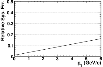
(f) Deuteron Tagging

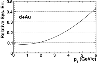
(g) Total d+Au Sys. Err.

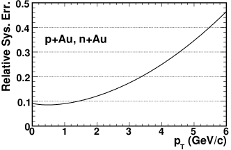
(h) Total N+Au Sys. Err.

Figure 13: Contributions to the systematic error associated with uncertainty in the various corrections. All errors are relative and represent a 90% confidence level. The total systematic error is the quadrature sum of the individual contributions.

Systematics of the Centrality Measurements

In depth studies of the accuracy with which centrality parameters like $N_{\rm part}$ could be estimated were performed prior to this analysis, as described in [92]. First, the dependence on the simulations was studied by varying the centrality efficiency and observing the effects on the estimated centrality parameter. The degree to which the centrality efficiency could vary was estimated by dividing the simulated data up into vertex bins and comparing the efficiency determined in each bin. Finally, the dependence on the deuteron wave function was studied by comparing the results of simulations performed using the Hulthen wave function shown in Eq. 5 to the results of simulations done using a Woods-Saxon distribution.

	Relative Systematic Error
Centrality Bin	$N_{\rm coll}$	$N_{\rm part}$	$N_{\rm part}^{Au}$	$N_{\rm part}^{d}$	$\nu$
0-20%	6.1%	7.1%	7.4%	5.5%	6.1%
20-40%	7.1%	8.3%	7.9%	5.3%	7.1%
40-70%	12.0%	11.1%	13.0%	12.0%	12.0%
70-100%	30.3%	22.4%	26.0%	16.7%	30.3%

Table 12: Systematic errors (90% C.L.) on the centrality parameters found with ERing and EOct cuts.

In addition, the dependence of the estimated centrality parameters on the specific collision model was studied. This was done by making a simple Glauber MC to find the distribution of each centrality parameter. This distribution was then scaled to match the data, the centrality cuts used on the data were then applied and the centrality parameter was extracted directly. This could then be compared to the result of the full centrality technique. To make the distribution obtained by the simple MC more realistic, further studies were done in which some Gaussian smearing was applied to the MC distributions. In addition, several different techniques were used to scale the MC distribution to match the data. Next, effects due to efficiency were taken into account by (a) scaling the MC distribution, (b) applying the efficiency to the distribution, (c) smearing the distribution, (d) correcting for the efficiency, (e) applying the centrality cuts and (f) extracting the average centrality parameter in each bin. Finally, other collision simulations were used to perform the full centrality procedure. The results of these studies are shown in Table 12.

These studies were done to estimate the systematic error on centrality parameters that were determined using similar techniques to those presented in this thesis. In fact, it is believed that the centrality technique described in Sect. 3 should be more accurate. Therefore, the systematic uncertainties shown in Table 12 were thought to provide a conservative estimate of the errors relevant to this analysis.

	Relative Systematic Error
Centrality Bin	$N_{\rm coll}$	$N_{\rm part}$	$N_{\rm part}^{Au}$	$N_{\rm part}^{d}$	$\nu$
0-20% d+Au	13.5%	10.7%	13.3%	5.9%	11.7%
p+Au	27.7%	23.1%	28.0%	5.5%	28.7%
n+Au	25.7%	23.1%	26.1%	5.5%	25.7%
[1pt/4pt] 20-40% d+Au	11.5%	11.5%	12.0%	6.6%	9.3%
p+Au	30.8%	27.3%	31.0%	5.3%	30.8%
n+Au	28.9%	27.3%	30.1%	5.3%	28.9%
[1pt/4pt] 40-70% d+Au	14.4%	13.7%	15.8%	13.4%	13.9%
p+Au	29.5%	24.6%	30.9%	12.0%	29.5%
n+Au	29.5%	24.6%	30.9%	12.0%	29.5%
[1pt/4pt] 70-100% d+Au	31.0%	23.0%	26.7%	16.7%	30.1%
p+Au	30.0%	22.4%	26.0%	16.7%	30.0%
n+Au	30.1%	22.5%	26.1%	16.7%	30.1%

Table 13: Total systematic uncertainties (90% C.L.) associated with EPCAL based centrality cuts.

However, additional systematic errors were needed to estimate uncertainties in the new centrality procedure used to find parameters (like $N_{\rm part}$) in EPCAL bins described in Sect. 3. These uncertainties were estimated by applying the procedure to a variable for which the centrality parameters could be determined in the more traditional manner. For example, the $N_{\rm part}$ estimated using EOct centrality cuts could be compared to the $N_{\rm part}$ estimated using the EOct cut values, but employing an “EOct from ERing” method to determine the average $N_{\rm part}$ value in the simulations. That is, centrality parameters were determined by the method described in Sect. 3, in which the observed correlation between EOct and ERing in the d+Au data was applied to the simulations. Discrepancies between the centrality parameters determined using the two methods gave an estimate of systematic biases introduced by the new technique.

In principal, these estimates could be used to correct for biases introduced onto the centrality parameters determined using EPCAL cuts. However, similar studies performed using different centrality measures produced different estimates of the systematic biases. This was also true for variations of existing centrality measures which were constructed to more closely approximate the EPCAL resolution. Since there was no specific centrality measure that was thought to provide a particularly accurate estimate (that is, a better estimate than any other measure) of the EPCAL systematics, no correction could be performed. Instead, these studies were used to determine the additional systematic uncertainty in the centrality parameters estimated by EPCAL centrality cuts. The total systematic uncertainties for EPCAL cuts are shown in Table 13.

Chapter 6 Spectra Measurements

After the raw transverse momentum spectra had been corrected, it was possible to measure the invariant charged hadron yield, as a function of transverse momentum, at an average pseudorapidity of 0.8 units (slightly forward in the deuteron direction). The spectra were measured in three different collision systems, d+Au, p+Au and n+Au, by the identification of nucleon-nucleus collisions described in Sect. 4. For each system, the $p_{\mathrm{T}}$ spectrum of positive hadrons, $\mathrm{h}^{+}$, negative hadrons, $\mathrm{h}^{-}$, and of the average, $(\mathrm{h}^{+}+\mathrm{h}^{-})/2$, was measured. Each spectrum was also measured in four bins of centrality. To study the effects of the centrality classification technique, six different variables were used as a centrality measure. Thus, a total of 216 spectra were measured.

Note that data presented for the first time in this thesis have not been reviewed by the PHOBOS collaboration.

1 Invariant Yield Data

The average hadron yield in d+Au, measured in four centrality bins by six different centrality measures, is shown in Fig. 1. Note that previous PHOBOS results [93] are different (by a few percent) from those presented in this thesis. The differences, while not big, are due to changes in both the data used and in the analysis procedure itself. A different data set, which included collisions recorded using a high-$p_{\mathrm{T}}$ trigger, was used in the former analysis. In addition, an antiquated and less efficient version of the PHOBOS Hough tracking procedure was used in that analysis.

The analysis procedure presented in this thesis further differed from the analysis of [93] in the way corrections were applied. In the former analysis, the acceptance and efficiency corrections were taken as smooth fits to the single track simulations, resulting in the removal of some of the features seen in Fig. 6 on page 6. In addition, corrections were not applied separately for each spectrometer arm; including both the acceptance and efficiency correction, as well as the dead and hot channel correction (which was in fact quite different for the two arms, see Sect. 3). Further, a subtle correction was needed in the former analysis to account for the vertex resolution. This correction was necessary because tracks were counted only between $\left|z\right|<10~{}\mbox{${\rm cm}$}$ based on the origin of the track, while collisions were counted in the same range, but based on the reconstructed vertex of the collision. This correction was avoided entirely in the analysis presented in this thesis by making both cuts using the vertex of the collision.

Finally, the method of centrality determination was different in the analysis presented in [93]. In that work, ERing cuts were determined using HIJING, rather than AMPT. Because the ERing distribution in HIJING did not have the same shape as in the data, it was not possible to determine centrality using the method described in Sect. 3. Instead, HIJING was used to determine the overall efficiency of the event selection and the average efficiency in each cross section bin. These average efficiencies were then assumed to be the same in the data, and were used to determine the appropriate centrality cuts. Since this method was unable to produce an event selection efficiency as a function of ERing, it was not possible for the former analysis to correct for that efficiency (see Sect. 4).

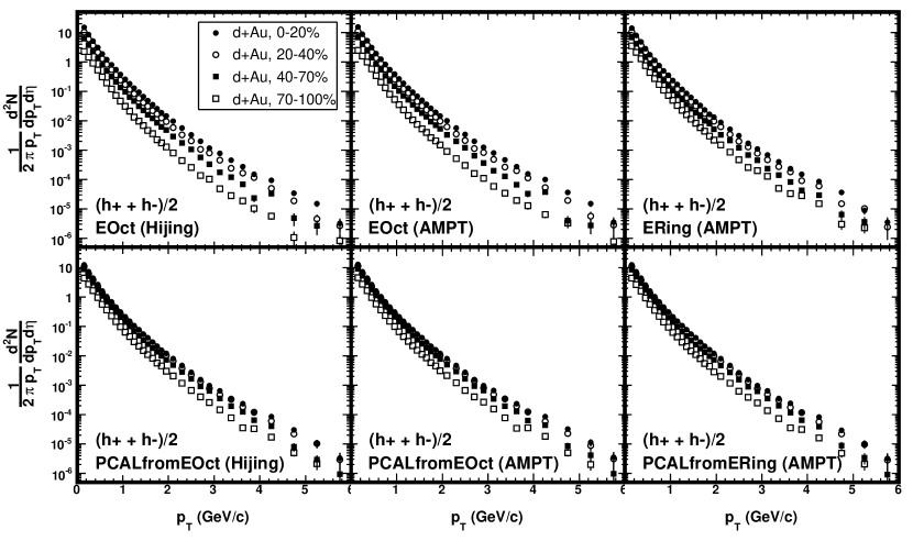
Figure 1: The invariant yield of charged hadrons emitted by d+Au collisions in four centrality bins. The variable used as the centrality measure is indicated in each plot. Only statistical errors are shown.

The positive, negative and average charged hadron spectra are shown in Fig. 2 for d+Au, p+Au and n+Au. Only the ERing centrality measure was used for these plots. Note that the difference in the $p_{\mathrm{T}}$ range between d+Au and the nucleon-nucleus spectra is due to statistics; fewer p+Au and n+Au collisions were collected.

Figure 2: The invariant yield of $(\mathrm{h}^{+}+\mathrm{h}^{-})/2$, $\mathrm{h}^{+}$ and $\mathrm{h}^{-}$ in four centrality bins determined using the ERing centrality variable. The spectra for d+Au, n+Au and p+Au are shown in separate columns. Only statistical errors are shown.

2 Fitting the Spectra

The charged hadron spectra were fit using the sum of an exponential in transverse mass, $m_{\mathrm{T}}=\sqrt{m^{2}+p_{\mathrm{T}}^{2}}$, and a power law in transverse momentum. These choices were motivated only loosely by physics. That is, the essential functional form of the fit was borrowed from previous physical arguments, but the fit parameters were not treated as physically meaningful. The only goal was to obtain a good fit to the data. The exponential term was inspired by theoretical arguments for the production of soft (low $p_{\mathrm{T}}$) hadrons, both in nucleon-nucleon collisions [101] and in nucleus-nucleus collisions [102]. Since the unidentified hadron spectra were composed primarily of pions [29], the charged pion mass, $m_{\pi}=0.13957~{}\mbox{${\rm GeV}$}$, was used to calculate $m_{\mathrm{T}}$. The power law term of the fit was taken from leading-order perturbative QCD calculations of jet production in heavy ion collisions [103]. This makes it primarily relevant for the hard part of the spectrum (above a few GeV$\kern-1.49994pt/\kern-1.19995ptc$). However, previous empirical observations have shown that such a power law fit well to nucleon-nucleon data over a wide range of transverse momentum [104]. The full form of the function used to fit the spectra was as follows.

$$\frac{1}{2\pi p_{\mathrm{T}}}\frac{d^{2}\!N}{\mathit{dp_{\mathrm{T}}}\mathit{d\eta}}=A\left(1+\frac{p_{\mathrm{T}}}{p_{0}}\right)^{-n}+B\exp\left(\frac{-\sqrt{p_{\mathrm{T}}^{2}+m_{\pi}^{2}}}{T}\right)$$ (1)

An observable used extensively in the analysis presented in this thesis was the integral of the spectra over $p_{\mathrm{T}}$; that is, the average $d\!N/\mathit{d\eta}$ at $\eta=0.8$. This integral was obtained directly from the fit to the data. Because Eq. 1 could be integrated analytically, it was possible to redefine one of the fit parameters, namely $A$, in terms of the integral of the function (and the other fit parameters).

$$\frac{d\!N}{\mathit{d\eta}} =\int_{0}^{+\infty}2\pi p_{\mathrm{T}}\left[A\left(1+\frac{p_{\mathrm{T}}}{p_{0}}\right)^{-n}+B\exp\left(\frac{-\sqrt{p_{\mathrm{T}}^{2}+m_{\pi}^{2}}}{T}\right)\right]d\!p_{\mathrm{T}}$$ (2)

$$\equiv I_{\mathrm{pl}}+I_{\mathrm{exp}}$$

Integrating the power-law term first:

$$I_{\mathrm{pl}} =\int_{0}^{+\infty}\left(2\pi p_{\mathrm{T}}\right)A\left(1+\frac{p_{\mathrm{T}}}{p_{0}}\right)^{-n}d\!p_{\mathrm{T}}$$

$$=2\pi A\int_{1}^{+\infty}p_{0}^{2}(u-1)u^{-n}d\!u\qquad\text{where}\quad u=1+\frac{p_{\mathrm{T}}}{p_{0}}$$

$$=2\pi Ap_{0}^{2}\left[\left[\frac{1}{1-n}u^{1-n}(u-1)\right]_{1}^{+\infty}-\frac{1}{1-n}\int_{1}^{+\infty}u^{1-n}d\!u\right]\qquad\text{by parts}$$

$$=2\pi Ap_{0}^{2}\left[0+\frac{1}{n-1}\left[\frac{1}{2-n}u^{2-n}\right]_{1}^{+\infty}\right]$$

$$I_{\mathrm{pl}} =2\pi Ap_{0}^{2}\frac{1}{(n-1)(n-2)}$$ (3)

where it is assumed that $n>2$. Similarly, the exponential term can be integrated.

$$I_{\mathrm{exp}} =\int_{0}^{+\infty}\left(2\pi p_{\mathrm{T}}\right)B\exp\left(\frac{-\sqrt{p_{\mathrm{T}}^{2}+m_{\pi}^{2}}}{T}\right)d\!p_{\mathrm{T}}$$

$$=2\pi B\int_{m_{\pi}}^{+\infty}\left(m_{\mathrm{T}}e^{-m_{\mathrm{T}}/T}\right)d\!m_{\mathrm{T}}$$

$$I_{\mathrm{exp}} =2p_{\mathrm{T}}BT(m_{\pi}+T)e^{-m_{\pi}/T}\qquad\text{by parts}$$ (4)

Using Eq. 3 and 4, the fit parameter $A$ of Eq. 2 can be defined in terms of the physical variable $d\!N/\mathit{d\eta}$.

$$\frac{d\!N}{\mathit{d\eta}} =I_{\mathrm{pl}}+I_{\mathrm{exp}}$$

$$=\frac{2\pi Ap_{0}^{2}}{(n-1)(n-2)}+2\pi BT(m_{\pi}+T)e^{-m_{\pi}/T}$$

$$\Longleftrightarrow A =\frac{(n-1)(n-2)}{2\pi p_{0}^{2}}\left[\frac{d\!N}{\mathit{d\eta}}-2\pi BT(m_{\pi}+T)e^{-m_{\pi}/T}\right]$$

This allows Eq. 2 to be re-written as

$$\frac{1}{2\pi p_{\mathrm{T}}}\frac{d^{2}\!N}{\mathit{dp_{\mathrm{T}}}\mathit{d\eta}}=\frac{(n-1)(n-2)}{2\pi p_{0}^{2}}\left[\frac{d\!N}{\mathit{d\eta}}-2\pi BT(m_{\pi}+T)e^{-m_{\pi}/T}\right]\left(1+\frac{p_{\mathrm{T}}}{p_{0}}\right)^{-n}\\ +B\exp\left(\frac{-\sqrt{p_{\mathrm{T}}^{2}+m_{\pi}^{2}}}{T}\right)$$ (5)

Parameter	Minimum	Maximum
$d\!N/\mathit{d\eta}$	0	92
$T$	0 ${\rm GeV}$	0.500 ${\rm GeV}$
$B$	0	40
$p_{0}$	0 GeV$\kern-1.49994pt/\kern-1.19995ptc$	4 GeV$\kern-1.49994pt/\kern-1.19995ptc$
$n$	6	17

Table 1: The ranges over which parameters were varied while fitting the spectra.

The advantage of Eq. 5 is that it contains a physically meaningful fit parameter, namely $d\!N/\mathit{d\eta}$. This was the function fit to the transverse momentum spectra. The ranges over which the fit parameters were varied are shown in Table 1. The multiplicity and the statistical error on the multiplicity measurement were then extracted directly from the fit.

As a cross-check on the $d\!N/\mathit{d\eta}$ value obtained from the fit, an estimate of $d\!N/\mathit{d\eta}$ was calculated from the data. This was done by finding the integral of the data in the most straight-forward way. First, the content of each $p_{\mathrm{T}}$ bin was multiplied by $2\pi p_{\mathrm{T}}W_{b}$, where $W_{b}$ is the width of the $p_{\mathrm{T}}$ bin. Then the sum, $S_{b}$, of these terms for each $p_{\mathrm{T}}$ bin was obtained. Finally, the spectra was extrapolated to $p_{\mathrm{T}}=0~{}\mbox{\rm GeV$\kern-1.49994pt/\kern-1.19995ptc$}$ by calculating a straight line from the two lowest $p_{\mathrm{T}}$ data points. The integral of this line (below the lowest $p_{\mathrm{T}}$ bin) was then added to the sum $S_{b}$. The resulting total provided a rough estimate of $d\!N/\mathit{d\eta}$. Typically, this value differed from the $d\!N/\mathit{d\eta}$ obtained from the fit by about 1%. The two estimates always agreed to better than 5%.

The systematic uncertainty on the integrated yield was determined using the following method. First, all points of a given measured spectrum were shifted up to the maximum of their systematic error. Then, this new $p_{\mathrm{T}}$ spectrum was fit and a maximum $d\!N/\mathit{d\eta}$ value was obtained. Next, all points on the spectrum were shifted down to the minimum of their systematic error. Again, this new spectra was fit and a minimum $d\!N/\mathit{d\eta}$ value was extracted. Using this method, it was found that the minimum and maximum integrated yields were consistently within about 9% of the measured integrated yield. Thus, a relative systematic uncertainty (90% C.L.) on the integrated yield of 9% was determined. This error was found to be independent of centrality bin, centrality measure, the specific hadron spectra (i.e. average or charged hadrons) and the collision system.

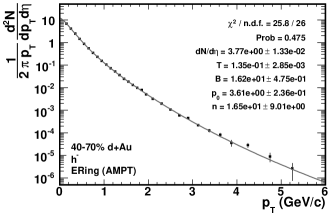
(a) $\mathrm{h}^{-}$ Fit

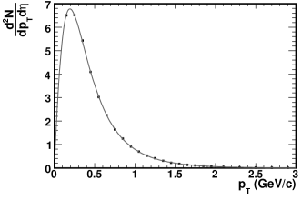
(b) $\mathrm{h}^{-}$ Fit (Linear)

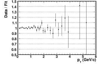
(c) Data / Fit Ratio

Figure 3: An example of a good fit to spectra that was generated with a large number of tracks. 3(a) The fit of the $\mathrm{h}^{-}$ spectra in the 40-70% most central d+Au (as found using the ERing centrality variable). 3(b) The transverse momentum distribution (not invariant yield) and fit on a linear scale. Note the smaller $p_{\mathrm{T}}$ range displayed. 3(c) Ratio of the data to the fit.

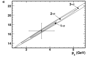
(a) $n$ vs $p_{0}$

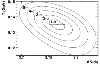
(b) $T$ vs $d\!N/\mathit{d\eta}$

Figure 4: The $\chi^{2}$ contours for the fit to the 40-70% most central $\mathrm{h}^{-}$ spectra in d+Au. The sigma contours are labeled, and the points show the minima found by the fit. 4(a) The $n$ and $p_{0}$ parameter space. The correlation between these two parameters is evident. 4(b) The $T$ and $d\!N/\mathit{d\eta}$ parameter space.

An example of a fit to the measured spectra can be seen in Fig. 3. The spectra shown in Fig. 3 has good statistics; that is, it was produced using a large number of tracks over much of the $p_{\mathrm{T}}$ range (around 142,000 total). The transverse momentum distribution of particles in the center of mass frame is shown in Fig. 3(b). This spectra was fit well by Eq. 5, as seen by both the fit probability (see Fig. 3(a)) and the ratio of the data to the fit (see Fig. 3(c)). As noted in the UA1 paper [104], the parameters $p_{0}$ and $n$ are highly correlated. This can be seen in Fig. 4(a), which shows the first three $\chi^{2}$ contours for these variables, as determined for the fit shown in Fig. 3. However, the $d\!N/\mathit{d\eta}$ parameter does not show a strong correlation with the other parameters; see Fig. 4(b) for the $\chi^{2}$ contours in the $T-d\!N/\mathit{d\eta}$ plane. Thus, it was assumed that the errors reported by the fit for $d\!N/\mathit{d\eta}$ were reasonable.

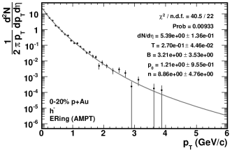
(a) $\mathrm{h}^{-}$ Fit

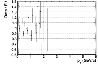
(b) Data / Fit Ratio

Figure 5: The fit of the $\mathrm{h}^{-}$ spectra in the 0-20% most central p+Au (as found using the ERing centrality variable). This is an example of a somewhat poor fit to spectra that was generated with a relatively small number of tracks.

An example of a fit to spectra that was produced with fewer tracks (around 3,400) is shown in Fig. 5. Despite the low statistics, fits to such spectra were not necessarily poor (as determined by $\chi^{2}$). However, the fit shown in Fig. 5 was intended to serve not only as an example of a fit to spectra with low statistics, but also as an example of an atypical (poor) fit.

3 Centrality Results

Six different centrality measures were used to find centrality cuts for the d+Au data. These measures were built from combinations of three variables (see Table 1 on page 1) and two MC simulations, HIJING and AMPT. The combinations are shown in Table 2. As described in Sect. 3, the MC simulations were used to estimate the efficiency of the trigger and event selection as a function of the centrality measure. To obtain this estimation, it was required that the shape of the centrality measure distribution in the simulations matched (possibly with some constant scaling factor) the same distribution observed in the collision data. Because such a matching could not be obtained for the ERing distribution in HIJING, ERing cuts using the HIJING simulations were not determined for this analysis.

Cut Variable	MC Simulation	Description
ERing	AMPT (8-18-03)	Energy in the Rings
EOct	AMPT (8-18-03)	Energy in the Octagon
EOct	HIJING (1.383)	Energy in the Octagon
EPCAL	AMPT (8-18-03)	Energy in the Au-PCAL, correlation with ERing used
EPCAL	AMPT (8-18-03)	Energy in the Au-PCAL, correlation with EOct used
EPCAL	HIJING (1.383)	Energy in the Au-PCAL, correlation with EOct used

Table 2: Description of centrality measures used in this analysis. See Sect. 3.

Each centrality measure was used to find centrality cuts corresponding to fractional cross section bins containing the 0-20%, 20-40%, 40-70% and 70-100% most central d+Au collisions. The cuts determined for the EOct centrality measure, using HIJING simulations, are shown in Fig. 9 on page 9. These same cuts were used for the nucleon-nucleus collision systems p+Au and n+Au. However, the fraction of the nucleon-nucleus cross section to which the bins corresponded was left undetermined (see Sect. 3). The average unbiased $N_{\rm part}$ estimated for each centrality bin of each centrality measure is shown in Table 3.

d+Au unbiased $N_{\rm part}$ with dAuSpectra event selection
		$\left<N_{\rm part}\right>\pm\text{Sys. Err.}$
Variable	Simulation	70-100%	40-70%	20-40%	0-20%
EOct	HIJING	$3.73\pm 0.84$	$7.48\pm 0.83$	$11.32\pm 0.94$	$15.15\pm 1.08$
EOct	AMPT	$3.75\pm 0.84$	$7.52\pm 0.83$	$11.28\pm 0.94$	$15.02\pm 1.07$
ERing	AMPT	$3.12\pm 0.70$	$6.31\pm 0.70$	$10.62\pm 0.88$	$15.42\pm 1.09$
EPCAL (EOct)	HIJING	$5.31\pm 1.22$	$8.25\pm 1.13$	$10.49\pm 1.21$	$12.19\pm 1.30$
EPCAL (EOct)	AMPT	$5.26\pm 1.21$	$8.30\pm 1.14$	$10.46\pm 1.21$	$12.07\pm 1.29$
EPCAL (ERing)	AMPT	$4.12\pm 0.94$	$7.36\pm 1.01$	$10.43\pm 1.20$	$12.82\pm 1.37$

Table 3: d+Au unbiased $N_{\rm part}$ obtained using different centrality measures and the dAuSpectra event selection.

The widths of the d+Au centrality bins used in this analysis were the same as those used in the previous PHOBOS d+Au $p_{\mathrm{T}}$ spectra analysis [93]. However, neither the procedure to determine the centrality bins nor the MC simulations used were the same between the two analyses. In addition, all centrality parameters (such as $N_{\rm part}$) used in the analysis presented in this thesis were unbiased. That is, the estimated trigger and event selection efficiency was used to correct for biases introduced by the centrality dependence of the efficiency, as described in Sect. 2. Thus the average $N_{\rm part}$ values estimated in the two analyses were not expected to be identical (although they do agree within systematic uncertainties). A comparison of the biased and unbiased $N_{\rm part}$ values estimated for the ERing centrality cuts found using AMPT simulations is shown in Table 4. Note that the average $N_{\rm part}$ in the central bins are essentially the same, which is reasonable since the efficiency was independent of centrality in this region (see Fig. 9 on page 9). However, the efficiency was found to decrease with decreasing centrality, and the resulting bias can be seen in the average $N_{\rm part}$ values estimated for the two peripheral bins.

d+Au $N_{\rm part}$ with dAuSpectra event selection
		$\left<N_{\rm part}\right>\pm\text{Sys. Err.}$
Variable	Type	70-100%	40-70%	20-40%	0-20%
ERing	Unbiased	$3.12\pm 0.70$	$6.31\pm 0.70$	$10.62\pm 0.88$	$15.42\pm 1.09$
ERing	Biased	$3.43\pm 0.77$	$6.50\pm 0.72$	$10.66\pm 0.88$	$15.44\pm 1.10$

Table 4: Biased and unbiased $N_{\rm part}$ values obtained using ERing, AMPT and the dAuSpectra event selection.

In addition to the two centrality parameters shown in Fig. 5 on page 5, $N_{\rm part}$ and $N_{\rm coll}$, three other parameters were studied in the MC. Two were simple components of $N_{\rm part}$. Both the average number of deuteron participants ($N_{\rm part}^{d}$) and the average number of participating gold nucleons ($N_{\rm part}^{Au}$) were estimated for each centrality bin. The fifth centrality parameter was particularly useful for describing the geometry of d+Au collisions. It was defined as the number of collisions per deuteron participant, $\nu\equiv N_{\rm coll}/N_{\rm part}^{d}$ [91]. The average unbiased $\nu$ estimated for each centrality bin of each centrality measure is shown in Table 6. Note that $\left<\nu\right>$ was estimated by finding the average of the ratio $N_{\rm coll}/N_{\rm part}^{d}$ in the simulated collisions, rather than taking the ratio of $\left<\smash[tb]{N_{\rm coll}}\right>/\left<\smash[tb]{N_{\rm part}^{d}}\right>$. The average of each centrality parameter in each d+Au centrality bin as found using ERing and AMPT is shown in Table 5.

d+Au centrality parameters found with ERing cuts
	$\left<\text{Parameter}\right>\pm\text{Sys. Err.}$
Parameter	70-100%	40-70%	20-40%	0-20%
$\left<\smash[b]{N_{\rm coll}}\right>$	$2.00\pm 0.60$	$4.99\pm 0.60$	$9.43\pm 0.67$	$14.49\pm 0.88$
$\left<\smash[b]{N_{\rm part}}\right>$	$3.12\pm 0.70$	$6.31\pm 0.70$	$10.62\pm 0.88$	$15.42\pm 1.09$
$\left<\smash[tb]{N_{\rm part}^{Au}}\right>$	$1.92\pm 0.50$	$4.64\pm 0.60$	$8.70\pm 0.69$	$13.43\pm 0.99$
$\left<\smash[tb]{N_{\rm part}^{d}}\right>$	$1.20\pm 0.20$	$1.67\pm 0.20$	$1.93\pm 0.10$	$1.99\pm 0.11$
$\left<\nu\right>$	$1.73\pm 0.52$	$3.27\pm 0.39$	$5.20\pm 0.37$	$7.55\pm 0.46$

Table 5: Unbiased centrality parameters obtained using ERing, AMPT and the dAuSpectra event selection.

d+Au unbiased $\nu$ with dAuSpectra event selection
		$\left<\nu\right>\pm\text{Sys. Err.}$
Variable	Simulation	70-100%	40-70%	20-40%	0-20%
EOct	HIJING	$2.06\pm 0.62$	$3.84\pm 0.46$	$5.56\pm 0.39$	$7.47\pm 0.46$
EOct	AMPT	$2.06\pm 0.62$	$3.80\pm 0.46$	$5.51\pm 0.39$	$7.37\pm 0.45$
ERing	AMPT	$1.73\pm 0.52$	$3.27\pm 0.39$	$5.20\pm 0.37$	$7.55\pm 0.46$
EPCAL (EOct)	HIJING	$2.80\pm 0.84$	$4.18\pm 0.58$	$5.23\pm 0.49$	$6.04\pm 0.71$
EPCAL (EOct)	AMPT	$2.75\pm 0.83$	$4.17\pm 0.58$	$5.19\pm 0.48$	$5.95\pm 0.70$
EPCAL (ERing)	AMPT	$2.20\pm 0.66$	$3.73\pm 0.52$	$5.17\pm 0.48$	$6.30\pm 0.74$

Table 6: d+Au unbiased $\nu$ obtained using different centrality measures and the dAuSpectra event selection.

Chapter 7 Studies of d+Au, p+Au and n+Au Spectra

With the measured spectra fully corrected, it was possible to study particle production in p+Au, n+Au and d+Au collisions at a center of mass energy of 200 ${\rm GeV}$ per nucleon pair. The extreme asymmetry of these collision systems, in addition to the small transverse area of the interaction region (as compared to Au+Au), necessitated a clear understanding of the centrality of the collisions. To this end, the impact of the choice of centrality measure on the spectra measurement was investigated. Further studies of the transverse momentum spectra were then conducted. First, the assumption that d+Au collisions rather than nucleon-nucleus collisions could be used as a control experiment for Au+Au, in the sense of a collision system that includes nuclear effects but not any extended volume medium effects, was tested. Then, a systematic study of the modification of hadron production in d+Au with respect to p+p̄ was performed. This study examined the change in shape of the spectrum, both as a function of the amount of initial nuclear material probed by the deuteron and as a function of the outgoing particle density. Finally, charged hadron production in p+Au was compared to production in n+Au.

Note that data presented for the first time in this thesis have not been reviewed by the PHOBOS collaboration.

1 Significance of the Chosen Centrality Technique

It has been generally accepted that the technique used to determine and to parameterize the centrality of collisions can impact the desired measurement; see for example [105] and [106]. Precisely how measurements of particle production in d+Au and nucleon-nucleus collisions were affected by the techniques discussed in Sect. 3 was studied.

1 Fractional Cross Section

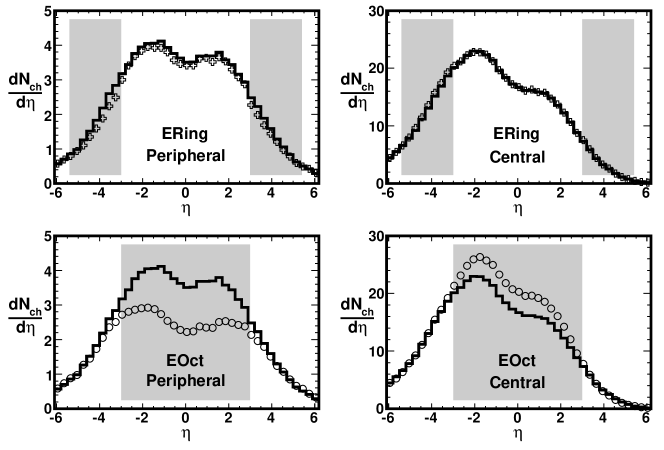
Figure 1: The bias introduced by the choice of centrality measure. Reconstructed d+Au multiplicity distributions in HIJING are shown by the open symbols. The unbiased, true multiplicity distribution is shown by the solid line. Shaded areas indicate the pseudorapidity region over which the centrality variable is measured [30].

The PHOBOS experiment used a multiplicity-based measurement, the amount of energy deposited into the Paddles [107], to determine the centrality of Au+Au collisions. Similar multiplicity-based measurements were used to classify the centrality of d+Au collisions. However, it was found that in d+Au, special care had to be taken to ensure that the choice of centrality measure did not bias the physics analysis. As discussed in [30], different biases were observed for centrality variables that used data from different ranges of pseudorapidity. This can be seen by comparing the reconstructed multiplicity distributions to the true distributions in HIJING collisions, for both EOct and ERing centrality cuts. As shown in Fig. 1 [30], centrality cuts based on the ERing variable produced little or no bias on the multiplicity reconstructed in the central pseudorapidity region. On the other hand, centrality cuts based on EOct did bias the reconstructed multiplicity. The average peripheral collision, as selected by EOct, was seen to have a lower multiplicity in the region of pseudorapidity over which EOct was measured than did the average unbiased collision in the same percent cross-section bin. The opposite was true for central collisions, where the average central collision selected by EOct had a higher multiplicity in the central region of pseudorapidity than did the average unbiased central collision.

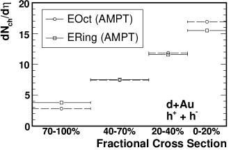
(a) $d\!N_{\mathrm{ch}}/\mathit{d\eta}$ vs Centrality Bin

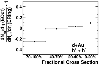
(b) $d\!N_{\mathrm{ch}}/\mathit{d\eta}$ Percent Difference

Figure 2: 2(a) The measured $d\!N_{\mathrm{ch}}/\mathit{d\eta}$ at $\left<\smash[b]{\eta}\right>=0.8$ as a function of fractional cross section for both EOct and ERing centrality cuts. Horizontal error bars represent the width of the bin. 2(b) The fractional difference between the integrated yield measured using ERing and EOct.

This biasing effect was also seen in the spectra data presented in this thesis. As shown in Fig. 2, the integrated yield measured in each centrality bin is dependent upon the choice of centrality measure. The $d\!N/\mathit{d\eta}$ values obtained from the fits to the $(h^{+}+h^{-})/2$ data were doubled, to obtain the integrated yield of all charged hadrons. The bias introduced by EOct centrality cuts on the (near mid-rapidity) integrated yield can be seen in Fig. 2(b). In peripheral events, the integrated yield measured using EOct cuts is lower than the integrated yield measured using ERing cuts, while in the most central events, the opposite effect is seen. This is the same bias observed in the HIJING simulations shown in Fig. 1. That the bias was observed both in HIJING simulations as well as in the data – with cuts made using efficiency estimates from AMPT – suggests that the effect is not somehow a product of the chosen model. Indeed, the integrated yield measured using EOct cuts found with HIJING agrees (to better than 10% in each centrality bin) with the integrated yield measured using cuts found with AMPT, as shown in Fig. 3.

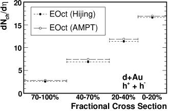
Figure 3: The measured $d\!N_{\mathrm{ch}}/\mathit{d\eta}$ at $\left<\smash[b]{\eta}\right>=0.8$ in EOct centrality bins is the same (within 10%) whether HIJING or AMPT was used to find the centrality cuts.

2 $N_{\rm part}$ Parametrization

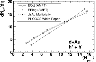
(a) $d\!N_{\mathrm{ch}}/\mathit{d\eta}$ vs $\left<\smash[b]{N_{\rm part}}\right>$

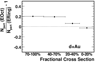
(b) $\left<\smash[b]{N_{\rm part}}\right>$ Percent Difference

Figure 4: 4(a) The measured $d\!N_{\mathrm{ch}}/\mathit{d\eta}$ at $\left<\smash[b]{\eta}\right>=0.8$ as a function of $\left<\smash[b]{N_{\rm part}}\right>$ for both EOct and ERing centrality cuts. The lines simply connect the data points to guide the eye. The data shown as asterisks are taken from [30]. Five centrality bins determined by ERing and HIJING were used for that analysis. 4(b) The percent difference in $\left<\smash[b]{N_{\rm part}}\right>$ as estimated using EOct and ERing centrality cuts.

Thus it is clear that the classification of d+Au interactions by fractional cross section does not select a unique set of collisions. However, it has been observed that the total charged particle multiplicity scales with the number of participating nucleons in hadron-nucleus [108, 109], deuteron-nucleus [110, 111] and heavy ion collisions [112]. Therefore, one may expect that the multiplicity near mid-rapidity may be more accurately parametrized by $N_{\rm part}$, rather than by fractional cross section.

The integrated yield of charged hadrons is shown as a function of $\left<\smash[b]{N_{\rm part}}\right>$ for two different centrality measures in Fig. 4(a). The data labeled “d+Au Multiplicity” were taken from [30]. To ensure that the data from the multiplicity measurement were compatible with the data from the spectra analysis, the pseudorapidity range of the spectra had to be accounted for. This was done by averaging the multiplicity measurements of $d\!N/\mathit{d\eta}$ at $\eta=0.7$ and $\eta=0.9$, to match the $d\!N/\mathit{d\eta}$ at $\left<\smash[b]{\eta}\right>=0.8$ obtained from the spectra. The multiplicity measurement used ERing as the centrality measure, but used HIJING simulations to estimate $N_{\rm part}$. As seen in Fig. 4(a), the multiplicity measurement from [30] agrees quite well with the $d\!N/\mathit{d\eta}$ obtained from the spectra analysis using ERing cuts. Such a comparison of the two results provides an important cross-check on the two independent analyses, and adds confidence in the accuracy of the results.

With centrality parametrized by $N_{\rm part}$, the bias on the integrated yield reconstructed with EOct centrality cuts remains. Indeed it must, since while the integrated yield reconstructed in the most peripheral EOct bin was lower than in the same ERing bin (see Fig. 2(b)), the average number of participants was estimated to be larger in the peripheral EOct bin than in the peripheral ERing bin, as shown in Fig. 4(b) and Table 3 on page 3. $N_{\rm part}$ being larger in the most peripheral EOct bin and smaller in the most central EOct bin, as compared to the corresponding ERing bins, is a consequence of the poorer $N_{\rm part}$ resolution predicted by the models for EOct as compared to ERing. That is, collisions with the same $N_{\rm part}$ will have a wider spread in EOct values than in ERing values. These fluctuations tend to diminish the distinction between the average number of participants in neighboring centrality bins.

3 Two-Component Parametrization

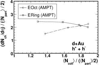
(a) Two-Component Parametrization

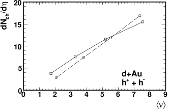
(b) $d\!N_{\mathrm{ch}}/\mathit{d\eta}$ vs $\left<\nu\right>$

Figure 5: 5(a) The measured $d\!N_{\mathrm{ch}}/\mathit{d\eta}$ per participant pair at $\left<\smash[b]{\eta}\right>=0.8$ as a function of $\left<\smash[b]{N_{\rm coll}}\right>/(\left<\smash[b]{N_{\rm part}}\right>/2)$. The integrated yield bias from EOct centrality cuts is not resolved by the two-component parametrization. 5(b) $d\!N_{\mathrm{ch}}/\mathit{d\eta}$ as a function of $\left<\nu\right>$.

While the total multiplicity in various collision systems has been shown to scale with the number of participants, the mid-rapidity multiplicity in heavy ion collisions at $\sqrt{s_{\scriptscriptstyle{{\rm NN}}}}=200~{}\mbox{${\rm GeV}$}$ is better described by a two-component model [31]. The motivation for such a model came from the expectation that as the collision energy increases, hard-scattering (i.e. jet production) becomes more important; however see [31] for a measurement of the magnitude of this effect. Further, processes such as jet production are expected to scale with the number of inelastic collisions in the absence of final state effects (such as energy loss of produced particles traveling through a dense medium). Thus, a two component parametrization of the mid-rapidity multiplicity of heavy ion collisions was proposed [113, 114]

$$\frac{d\!N_{\mathrm{ch}}}{\mathit{d\eta}}=n_{\mathrm{pp}}\left[(1-x)(\left<\smash[b]{N_{\rm part}}\right>/2)+x\left<\smash[b]{N_{\rm coll}}\right>\right]$$ (1)

where $n_{\mathrm{pp}}$ is the multiplicity in p+p and $x$ is the fraction of charged particle production due to hard scattering processes. This implies that the mid-rapidity multiplicity per participant pair should scale with the number of collisions per participant pair

$$\frac{1}{\left<\smash[b]{N_{\rm part}}\right>/2}\frac{d\!N_{\mathrm{ch}}}{\mathit{d\eta}} =n_{\mathrm{pp}}\left[(1-x)+x\frac{\left<\smash[b]{N_{\rm coll}}\right>}{\left<\smash[b]{N_{\rm part}}\right>/2}\right]$$ (2)

since both $n_{\mathrm{pp}}$ and $x$ are independent of centrality. The integrated yield per participant pair measured in d+Au collisions by the spectra analysis using both EOct and ERing cuts as a function of $\left<\smash[b]{N_{\rm coll}}\right>/(\left<\smash[b]{N_{\rm part}}\right>/2)$ is shown in Fig. 5(a). It is clear that this parametrization does not account for the bias imposed on the integrated yield by the EOct cuts. The bias is also present when the centrality of d+Au collisions is parametrized by $\left<\nu\right>\equiv\left<\smash[tb]{N_{\rm coll}/N_{\rm part}^{d}}\right>$ [91], as seen in Fig. 5(b).

4 Au-PCAL Centrality Cuts

Centrality cuts based on the amount of spectator material should provide a reliable estimate of centrality parameters, such as $\left<\nu\right>$ [115]. This was the motivation for constructing the Au-PCAL; to measure the energy of spectator protons (those that did not suffer an inelastic collision) of the gold nucleus. However, unlike previous fixed target and emulsion experiments that could directly observe such particles [115, 116, 88, 117, 118], the PHOBOS Au-PCAL was, for a number of reasons, not able to count the number of spectator protons emerging from a collision. First, no tracking detectors were constructed to observe these particles; only the total energy was measured. Second, this energy was seen to fluctuate significantly for collisions of a similar centrality (see Fig. 12(a) on page 12(a)). Simulations of single nucleons traveling at or near beam rapidity suggested that the fluctuations had two main sources. One was leakage of the neutron-induced hadron shower in the ZDC into nearby Au-PCAL modules. The other was due to the passage of protons through a significant amount of iron as they were bent out of the DX-magnet, see Fig. 10(b) on page 10(b). Another possible source of fluctuations was related to the break-up of the nucleus, and was extremely difficult to simulate. As spectator protons leave the interaction region, they may be bound inside clusters such as deuterons or alpha particles. These clusters would have a different charge to mass ratio than a free proton, and would not be bent by the RHIC magnets into the Au-PCAL detector. Due to the difficulty of accurately simulating such processes, the magnitude of these effects was not determined.

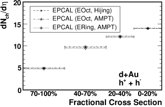
(a) EPCAL Cuts

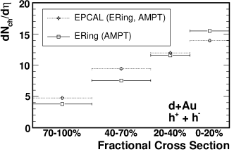
(b) EPCAL and ERing Cuts

Figure 6: 6(a) Comparison of the measured $d\!N_{\mathrm{ch}}/\mathit{d\eta}$ at $\left<\smash[b]{\eta}\right>=0.8$ obtained using EPCAL cuts with various correlations used to estimate efficiency. 6(b) The integrated yield reconstructed in EPCAL centrality bins compared to ERing centrality bins.

Despite these complications, there was no reason to suspect that centrality cuts based on EPCAL would cause any of the biasing effects seen with EOct cuts. That is, EOct was thought to bias measurements of multiplicity in the mid-rapidity region since EOct itself was a measurement of multiplicity in the mid-rapidity region. However, energy deposited in the Au-PCAL was not due to produced particles at all (having been shielded from such background, see Sect. 3) and therefore should not have biased measurements of produced particles. Thus it was expected that the multiplicity measured using EPCAL centrality cuts should be the same regardless of what MC simulation and variable were used to estimate the efficiency (see Sect. 3). This is indeed the case, as shown in Fig. 6(a). However, since the measurements presented in Fig. 6(a) were performed using the same data set, any differences in the measurements can only be due to differences in the efficiency estimates.

The integrated yield measured using EPCAL cuts, with efficiency estimated using ERing in AMPT simulations, is compared to the integrated yield measured using ERing cuts in Fig. 6(b). While both the EPCAL and ERing centrality measures are thought to impose little or no bias on the integrated yield measurement, the integrated yield in the most peripheral EPCAL bin is higher than that of the most peripheral ERing bin, and the opposite behavior is seen in the most central bin. One possible explanation for this is that the trigger and event selection efficiency may have been incorrectly estimated. This is almost certainly true for peripheral events, where fluctuations in the correlation between EPCAL and ERing resulted in a range of finite values of ERing in collisions that deposited no energy in the Au-PCAL, which in turn led to an unrealistically large estimate of the efficiency to detect collisions having very small values of EPCAL. In addition, large fluctuations in the EPCAL signal for collisions of similar centrality would reduce the centrality resolution of EPCAL, causing collisions in the peripheral bin of EPCAL to be more central than collisions in the peripheral bin of ERing.

(a) $\left<\smash[b]{N_{\rm part}}\right>$ Parametrization

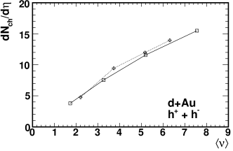
(b) $\left<\nu\right>$ Parametrization

Figure 7: Comparison of the measured $d\!N_{\mathrm{ch}}/\mathit{d\eta}$ at $\left<\smash[b]{\eta}\right>=0.8$ obtained using EPCAL and ERing centrality cuts. 7(a) Centrality is parametrized by $\left<\smash[b]{N_{\rm part}}\right>$. 7(b) Centrality is parametrized by $\nu$.

(a) EPCAL Cuts from EOct

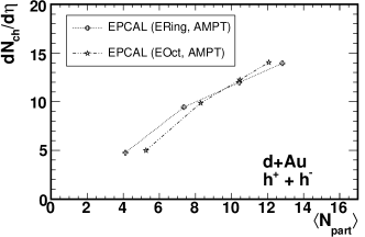
(b) Comparison of EPCAL Cuts

Figure 8: The measured $d\!N_{\mathrm{ch}}/\mathit{d\eta}$ at $\left<\smash[b]{\eta}\right>=0.8$ obtained using EPCAL centrality cuts. 8(a) The integrated yield in EPCAL bins determined using EOct follows the same trend as the integrated yield in EOct bins. 8(b) Estimates of $\left<\smash[b]{N_{\rm part}}\right>$ are biased by the choice of simulation variable used to estimate $\left<\smash[b]{N_{\rm part}}\right>$. Compare to Fig. 4(a).

Both of these effects lead to the conclusion that assigning fractional cross section widths to the centrality bins of EPCAL, found using the method described in Sect. 3, is suspect. Since the fractional cross section that each bin of EPCAL represents is not well determined, the centrality of the bins may be better described by collision geometry parameters such as $N_{\rm part}$. This indeed seems to be the case, as suggested by Fig. 7 which shows that the integrated yield measured in bins of EPCAL using ERing agrees with the integrated yield measured in bins of ERing. However, the integrated yield measured in bins of EPCAL that were determined using EOct in AMPT simulations, shown in Fig. 8(a), follow the same trend as the integrated yield measured in bins of EOct. This is not entirely surprising; it is not unreasonable to expect that the estimation of centrality parameters such as $\left<\smash[b]{N_{\rm part}}\right>$ was biased by the variable used in the simulations. This bias can be seen by comparing the integrated yield reconstructed in EPCAL centrality bins as a function of $\left<\smash[b]{N_{\rm part}}\right>$, where $\left<\smash[b]{N_{\rm part}}\right>$ was determined using either ERing or EOct in the simulations, as shown in Fig. 8(b) (compare to Fig. 4(a)). While studies were performed to try to correct for this bias on centrality parameters like $N_{\rm part}$, no reliable method for doing so was found.

5 Summary of Centrality Discussion

These studies make it clear that measurements of produced particles in the mid-rapidity region are biased, particularly in small systems, by centrality cuts placed on a variable that is itself a measure of mid-rapidity multiplicity. The bias was not found to depend on the choice of simulation model used to determine the triggering efficiency and the parameterizations of centrality (such as $N_{\rm part}$). The least biased centrality variable was found to be ERing, most likely due to the fact that it measures particles away from mid-rapidity. While it is believed that centrality cuts on EPCAL also impose little or no bias on measurements of produced particles near mid-rapidity, it was found that these fractional cross section cuts selected a different class of collisions than did fractional cross section cuts based on ERing or EOct. Further, attempts to describe the centrality of EPCAL bins by parameters like $N_{\rm part}$ were shown to preserve the bias of the centrality variable (i.e. EOct) used to estimate the average of the parameter in the MC simulations. That is, while the integrated yield reconstructed in EPCAL centrality bins may not itself have been biased, attempts to quantify the centrality of EPCAL bins were biased. For this reason, the majority of the discussion in this chapter will be on results found using ERing centrality cuts. Using these cuts gives a consistent set of results for d+Au, p+Au and n+Au collisions, as shown in Fig. 9 and discussed in the next section.

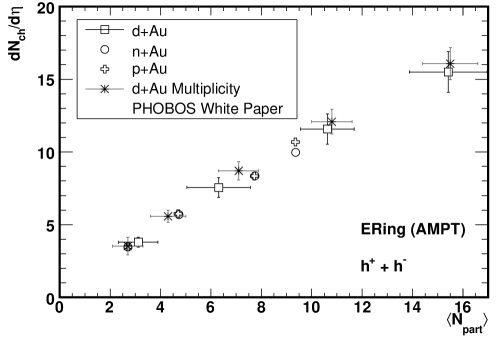
Figure 9: The measured $d\!N_{\mathrm{ch}}/\mathit{d\eta}$ at $\left<\smash[b]{\eta}\right>=0.8$ obtained using ERing centrality cuts. Systematic errors (90% C.L.) are shown for the d+Au measurements; statistical errors are negligible. Systematic errors on the nucleon-nucleus measurements are not shown, but are of similar order. A consistent dependence of the multiplicity on $N_{\rm part}$ is observed for the three different collision systems.

2 d+Au as a Control Experiment

The yield of hadrons in d+Au collisions played a vital role in the investigation of particle production in high energy Au+Au collisions [119]. In the absence of any nuclear or produced medium effects, a heavy ion collision would essentially be a collection of independent nucleon-nucleon collisions. In this naïve picture, the yield of an average Au+Au collision would be determined simply by the yield of an average nucleon-nucleon collision multiplied by the number of binary collisions taking place in the Au+Au system. The nuclear modification factor, $R_{X}$ given by Eq. 3, is therefore a convenient measure with which to test the assumption of binary collision scaling.

$$R_{X}=\frac{d^{2}\!N_{X}/\mathit{dp_{\mathrm{T}}}\mathit{d\eta}}{\left<\smash[b]{N_{\rm coll}}\right>d^{2}\!N_{\mathrm{NN}}/\mathit{dp_{\mathrm{T}}}\mathit{d\eta}}\qquad X=\text{\mbox{Au+Au}, \mbox{p+Au}, etc.}$$ (3)

This ratio was studied as a function of transverse momentum in order to separate soft processes from hard scattering processes. Previous studies of QCD have shown that short-range (hard processes) and long-range (soft processes) interactions factorize in the theory for simpler collision systems [120]. Assuming that factorization holds for high energy nucleus-nucleus collisions, binary collision scaling should be expected for large momentum transfer collisions that produce high-$p_{\mathrm{T}}$ particles. For $N_{\rm coll}$ scaling to hold at high-$p_{\mathrm{T}}$, the chance for a hard scattering process to occur in a binary collision should not depend on the number of collisions either of the two nucleons had previously suffered. It is interesting to note that in Au+Au collisions at $\sqrt{s_{\scriptscriptstyle{{\rm NN}}}}=200~{}\mbox{${\rm GeV}$}$, the average number of collisions per participant has been estimated to be around 4.7 [113] to 5.2 [91]. The number of collisions suffered by the deuteron or proton in central d+Au or p+Au collisions, respectively, can be about 60% higher, however, as shown in Table 1. Note that the approximate scaling of the mid-rapidity multiplicity with $\left<\smash[b]{N_{\rm part}}\right>$, shown in Fig. 9, cannot be assumed to hold over a wide range of transverse momentum, since the multiplicity is dominated by low-$p_{\mathrm{T}}$ particles.

The nucleon-nucleon reference used for studies of heavy ion collisions at $\sqrt{s_{\scriptscriptstyle{{\rm NN}}}}=200~{}\mbox{${\rm GeV}$}$ came from the UA1 data [121] of the p+p̄ inelastic cross section. As described in [93], corrections were applied to the UA1 results to account for (a) the conversion from rapidity to pseudorapidity and (b) the difference between the UA1 acceptance ($\left|\smash[bt]{\eta}\right|<2.5$) and the PHOBOS acceptance ($0.2<\eta<1.4$). The p+p̄ reference spectrum was fit by the function

$$\frac{1}{2\pi p_{\mathrm{T}}}\frac{d^{2}\!N}{\mathit{dp_{\mathrm{T}}}\mathit{d\eta}}= \frac{50.9}{2\pi}\left(1+\frac{p_{\mathrm{T}}}{1.59}\right)^{-11.2}$$

$$\times\frac{p_{\mathrm{T}}}{\sqrt{p_{\mathrm{T}}^{2}+0.00545}}\qquad(y\rightarrow\eta)$$

$$\times\biggl{[}\frac{\ln\left(\exp(1.065+0.004p_{\mathrm{T}})^{\;40}+\exp(0.85+0.07p_{\mathrm{T}})^{\;40}\right)}{40}$$

$$\quad-0.12e^{-2p_{\mathrm{T}}}+0.04e^{-3.66p_{\mathrm{T}}}\biggl{]}\qquad(\text{acceptance correction})$$ (4)

The shape of the p+p̄ spectra described by Eq. 4 can be seen in Fig. 13(a). An inelastic p+p̄ cross section of 41 ${\rm mb}$ was used to estimate the yield of p+p̄ collisions given the differential cross section measurements from UA1.

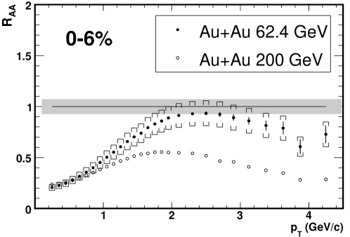
Figure 10: The nuclear modification factor measured by PHOBOS in the 0-6% most central Au+Au collisions. Brackets on $R_{AA}$ show the systematic uncertainties. The solid line shows the expectation of $N_{\rm coll}$ scaling and the grey band shows the systematic uncertainty on the overall scale due to $N_{\rm coll}$ [30].

The nuclear modification factor of nucleus-nucleus collisions at RHIC has been studied extensively for Au+Au interactions at $\sqrt{s_{\scriptscriptstyle{{\rm NN}}}}=62.4~{}\mbox{${\rm GeV}$}$ [122, 123], $130~{}\mbox{${\rm GeV}$}$ [124, 125, 126] and $200~{}\mbox{${\rm GeV}$}$ [127, 128, 129, 130], as well as for Cu+Cu interactions at $\sqrt{s_{\scriptscriptstyle{{\rm NN}}}}=62.4$ and $200~{}\mbox{${\rm GeV}$}$ [131]. As an example of these studies, the PHOBOS measurement of the nuclear modification factor in central Au+Au collisions, $R_{AA}$, at two center of mass energies is shown in Fig. 10 [30].

One of the fundamental conclusions drawn from examination of the nuclear modification factor was that the production of charged hadrons in central Au+Au collisions at $\sqrt{s_{\scriptscriptstyle{{\rm NN}}}}=200~{}\mbox{${\rm GeV}$}$ is highly suppressed with respect to binary collision scaling. This can be seen clearly in Fig. 10 [30]. However, it was not known from the nucleus-nucleus data alone whether the suppression was due to initial or final state effects. That is, were in fact fewer high-$p_{\mathrm{T}}$ hadrons being produced because of some modification of the initial nuclei, such as the one described in [132]? Or were the expected number of particles being produced, but losing energy during transit through some medium and being observed as lower-$p_{\mathrm{T}}$ hadrons, as described in [133]?

The hadron production of nucleon-nucleus collisions at the same center of mass energy could distinguish between the two possibilities. Any initial effects that modify the Au nucleus should still be present in N+Au interactions. On the other hand, final state effects caused by a dense medium in Au+Au collisions are not expected to be present in N+Au interactions, as the system size should be too small to produce a medium that high-$p_{\mathrm{T}}$ particles would interact with. Thus, N+Au collisions would serve as a control experiment for Au+Au interactions. At RHIC, these studies were performed using d+Au rather than N+Au collisions [93, 134, 135, 136, 137, 138]. This was due to technical reasons: the RHIC machine required mechanical changes in order to perform p+Au collisions (n+Au were not possible). However, the reasonable assumption was made that, due to the small size and weak binding of the deuteron nucleus, d+Au collisions would provide as good a control experiment for Au+Au interactions as N+Au collisions would.

1 $N_{\rm coll}$ Scaling from p+Au to d+Au

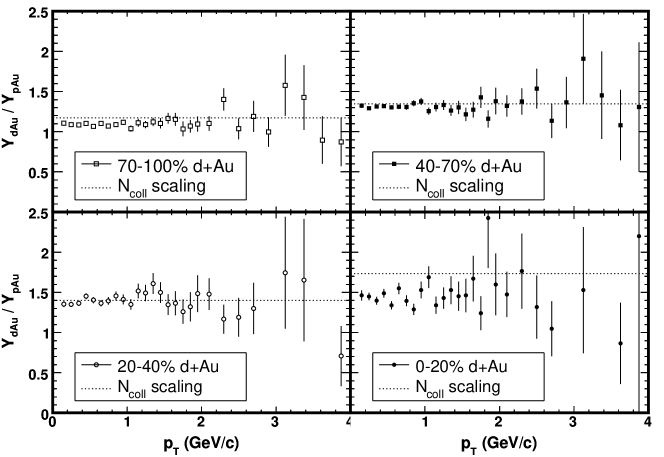
Figure 11: Ratio of the invariant yield of hadrons in d+Au collisions to the yield in p+Au collisions in each ERing centrality bin. The dotted line marks the expectation of $N_{\rm coll}$ scaling. Fractional cross section widths refer only to the d+Au cross section. See Table 1 for the relevant centrality parameters in each bin. Systematic errors not shown (see text).

Centrality Parameters in ERing Bins
Cent. Bin	$\left<b\right>$	$\left<\smash[b]{N_{\rm part}}\right>$	$\left<\smash[b]{N_{\rm coll}}\right>$	$\left<\nu\right>$	$d\!N/\mathit{d\eta}$
0-20% d+Au	$3.31$	$15.42\pm 1.09$	$14.49\pm 0.88$	$7.55\pm 0.46$	$15\pm 1.4$
p+Au	$6.09$	$9.36\pm 0.66$	$8.36\pm 0.51$	$8.36\pm 0.51$	$11\pm 0.99$
[1pt/4pt] 20-40% d+Au	$4.67$	$10.62\pm 0.88$	$9.43\pm 0.67$	$5.20\pm 0.37$	$12\pm 1.1$
p+Au	$6.38$	$7.72\pm 0.64$	$6.72\pm 0.48$	$6.72\pm 0.48$	$8.3\pm 0.75$
[1pt/4pt] 40-70% d+Au	$6.29$	$6.31\pm 0.70$	$4.99\pm 0.60$	$3.27\pm 0.39$	$7.6\pm 0.68$
p+Au	$7.18$	$4.70\pm 0.52$	$3.70\pm 0.44$	$3.70\pm 0.44$	$5.8\pm 0.52$
[1pt/4pt] 70-100% d+Au	$7.76$	$3.12\pm 0.70$	$2.00\pm 0.60$	$1.73\pm 0.52$	$3.8\pm 0.34$
p+Au	$8.01$	$2.71\pm 0.61$	$1.71\pm 0.51$	$1.71\pm 0.51$	$3.5\pm 0.32$

Table 1: Comparison of centrality parameters in each ERing bin for the d+Au and p+Au collision systems. Parameters of the n+Au collision system were found to be equivalent to those of the p+Au system. Errors represent systematic uncertainties (90% C.L.). The systematic error on impact parameter was not determined (the statistical uncertainty is negligible).

The analysis presented in this thesis provided a set of data with which this assumption could be tested. By using d+Au collisions to study the nuclear modification factor of a system with minimal final state effects, it was assumed implicitly that hadron production in d+Au interactions scale with $N_{\rm coll}$ relative to N+Au. Figure 11 shows the ratio of the average charged hadron yield in d+Au collisions to the yield in p+Au collisions. The dotted line shows the expectation of $N_{\rm coll}$ scaling. Systematic errors on the spectra measurements are not shown in this figure, as they are expected to be highly correlated between d+Au and p+Au, and are thus unnecessary for the comparison of the systems. While it was also expected that a strong correlation exists between systematic uncertainties in the number of collisions in the two systems, the magnitude of correlation was not determined. Therefore, the correct systematic uncertainty in the ratio of $N_{\rm coll}$ is not well understood.

The ratio of the yields was taken between spectra in a given ERing centrality bin. Recall that the fractional cross section included in a centrality bin was estimated only for d+Au collisions, and not for p+Au collisions (see Sect. 3). Therefore, the average impact parameter of d+Au collisions may be quite different from that of p+Au collisions in the same ERing centrality bin. This was indeed the case, as seen in Table 1, which compares centrality parameters of the two systems in each bin.

The most extreme difference in impact parameter between the two systems occurred in the central bin. In the AMPT simulations, the impact parameter of the average p+Au collision in this bin was 80% larger than the average d+Au collision in the same bin. Since the impact parameter measured the distance between the center of the deuteron and the center of the gold nucleus, it is possible that the most central ERing bin contained d+Au collisions in which the nucleons of the deuteron were unusually far apart. The fact that, in the simulations at least, the proton of the average central p+Au collision suffered a comparable number of binary interactions as each deuteron nucleon in the average central d+Au collision provided further evidence for this situation.

While the simulations suggest a geometry of a central p+Au collision that is not thought to be physically unreasonable (large impact parameter and large deuteron “radius”), they may not provide an accurate simulation of the data. That is, there may be some effects, experimental or physical, present in the analysis of tagged p+Au collisions that were not present in the simulations. As discussed in Sect. 3, the fraction of d+Au collisions that were tagged as p+Au interactions was qualitatively different in the data and the simulations. The basic implication of this is that a larger number of very central p+Au collisions, relative to the number of d+Au collisions, were found in the data than in the simulations. Consequently, the average number of collisions estimated by the simulations for central p+Au interactions may have been too small, if the simulations were biased toward less central interactions. If this were indeed the case, then the expectation based on $N_{\rm coll}$ scaling shown in the central bin of Fig. 11 would be too large.

Thus, the data presented in Fig. 11 should not be interpreted as implying that central p+Au interactions were especially efficient at producing particles. Further studies into the reliability of the estimation of centrality parameters (like $N_{\rm coll}$) and of the tagging procedure in both the data and MC are required before such a statement can be made.

2 An Ideal $R_{AA}$ Reference

While no evidence was found of $N_{\rm coll}$ scaling violations between p+Au and d+Au interactions, the availability of p+Au and n+Au data allowed the construction of an ideal reference for Au+Au collisions. Previous studies performed by the NA49 collaboration [139, 140] have suggested that hadron production of nucleus-nucleus collisions may be better understood through careful consideration of the neutron content of the nucleus. With this in mind, an ideal nuclear modification factor variable may be defined as follows.

$$R_{NA}=\frac{0.40\left(Y_{pA}/\left<\smash[b]{N_{\rm coll}}\right>^{pA}\right)+0.60\left(Y_{nA}/\left<\smash[b]{N_{\rm coll}}\right>^{nA}\right)}{Y_{p\bar{p}}}$$ (5)

where $Y_{X}$ is the yield, $d\!N_{\mathrm{ch}}/\mathit{d\eta}$, in the specified collision system. The definition of $R_{NA}$ shown in Eq. 5 takes into account the fact that the gold nucleus consists of 60% neutrons and 40% protons.

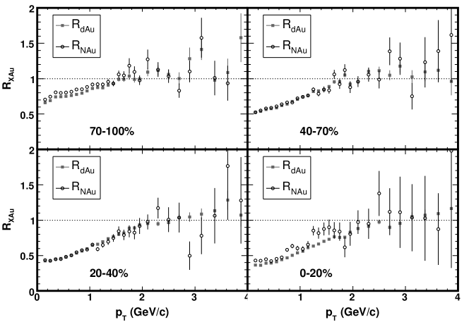
Figure 12: Comparison of $R_{dA}$ and $R_{NA}$, as defined by Eq. 5, in each ERing centrality bin. Systematic errors are not shown (see text).

The nuclear modification factor $R_{NA}$ is shown in Fig. 12. Also shown is $R_{dA}$, measured using the ERing centrality cuts. Systematic errors are not shown on this figure, as all systematic effects are expected to be highly correlated between d+Au and N+Au, and would therefore be unimportant to the comparison of the two systems. Systematic uncertainties in $N_{\rm coll}$ would affect the overall scale of the ratios and systematic uncertainties in the spectra measurements would tend to shift the d+Au and N+Au points by the same amount.

Not surprisingly, no significant difference between $R_{NA}$ and $R_{dA}$ is observed. However, this measurement bolsters the conclusions drawn from the nuclear modification factor measurements from d+Au collisions [30, 93]; namely, that high-$p_{\mathrm{T}}$ hadron production in central Au+Au collisions is significantly suppressed with respect to the expectation of binary collision scaling of p+p̄, while the production of d+Au collisions is not (compare Fig. 10 and 12). It should be noted that no claim of binary collision scaling in d+Au or N+Au interactions has been made. In addition to uncertainties on estimates of the number of collisions, it has been observed that the nuclear modification factor in d+Au exhibits a dependence on pseudorapidity [141, 138, 137, 123]. Thus, the apparent tendency of $R_{NA}$ and $R_{dA}$ to take the value of one at high-$p_{\mathrm{T}}$ is likely a consequence of the PHOBOS pseudorapidity acceptance. Further, as will be discussed in the next section, the hadron production of d+Au collisions is known to be enhanced with respect to binary collision scaling, in a certain range of transverse momentum. Any statement that d+Au lacks a suppression of high-$p_{\mathrm{T}}$ hadrons is therefore contingent upon the magnitude of this enhancement; see [142] for a discussion.

Nevertheless, the stark discrepancy between N+Au and Au+Au collisions at $\sqrt{s_{\scriptscriptstyle{{\rm NN}}}}=200~{}\mbox{${\rm GeV}$}$ demonstrate that final state effects play a much stronger role in the high-$p_{\mathrm{T}}$ hadron production of central Au+Au collisions than do initial state effects. While the pseudorapidity dependence of $R_{dA}$ may provide evidence of some initial modification of the gold nucleus [143, 144], it is clear that interactions with some dense, large volume medium produced only in the nucleus-nucleus system form the dominant source of high-$p_{\mathrm{T}}$ hadron suppression in Au+Au collisions. The data presented in this thesis prove that this conclusion was not biased by the the use of deuteron-nucleus rather than nucleon-nucleus interactions as the reference for Au+Au.

3 Centrality Dependence of Spectra

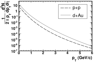
(a) Invariant Yields

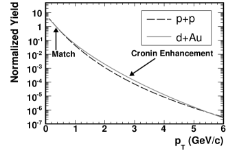
(b) Matched at Low $p_{\mathrm{T}}$

(c) Relative Yield vs $p_{\mathrm{T}}$

Figure 13: An example of the steps followed to determine the relative yield. 13(a) The invariant yield of d+Au compared to p+p̄. 13(b) The yields are scaled to match at $p_{\mathrm{T}}=0.35~{}\mbox{\rm GeV$\kern-1.49994pt/\kern-1.19995ptc$}$. The difference in shape of the two spectra is apparent. 13(c) The ratio of the scaled yields. The arrows mark the $p_{\mathrm{T}}$ values at which the centrality dependence of the relative yield was studied.

The shape of the nuclear modification factor seen in Fig. 10 and 12 is understood to be related to the so-called Cronin effect. This effect refers to the enhancement of hadron production in proton-nucleus collisions [145] relative to p+p collisions scaled by the effective thickness of the nucleus. General aspects of the enhancement of inclusive charged hadron production (that is, unidentified hadrons) in p+Au collisions can be described by models in which partons undergo multiple scattering at the initial impact of the p+Au collision [142]. However, the observed difference in the strength of enhancement for mesons and baryons [146] is not easily explained by initial state partonic scattering models. While other theories, such as those based on the recombination model of hadronization [147], may be better suited to describe the enhancement of individual hadron species, it remains safe to say that the Cronin effect is not a thoroughly understood phenomenon. Of particular importance in the study of this effect is the dependence of the enhancement on the nuclear thickness probed by the projectile (i.e. the deuteron in a d+Au collision) [148].

The centrality dependence of the nuclear modification factor in d+Au and Au+Au collisions at RHIC has been studied extensively [30, 149, 150, 151]. A particularly convenient method for exploring how the shape of the transverse momentum spectra changes relative to p+p̄ was suggested in [93]. This involved studying the centrality dependence of the charged hadron yield in d+Au collisions relative to p+p at several values of $p_{\mathrm{T}}$. The procedure for determining the so-called relative yield was as follows.

Figure 14: The average hadron yield of d+Au collisions relative to p+p̄ as a function of $\left<\smash[b]{N_{\rm coll}}\right>$. Statistical errors are represented by bars on the points. The systematic error (90% C.L.) for one group of points, EOct (HIJING), is shown by the grey band. See text for a discussion of the systematic errors. A dependence of the relative yield on both centrality and $p_{\mathrm{T}}$ is seen, but a bias introduced by the chosen centrality measure is also clearly visible.

First, the transverse momentum spectra in a particular d+Au centrality bin was compared to the spectra in p+p̄. An example of this is shown in Fig. 13(a). To compare only the shape of the two spectra, they were then normalized. As shown in Fig. 13(b), the d+Au spectra was matched to the p+p̄ spectra at $p_{\mathrm{T}}=0.35~{}\mbox{\rm GeV$\kern-1.49994pt/\kern-1.19995ptc$}$. While this specific value of $p_{\mathrm{T}}$ was arbitrary, it was intentionally chosen to be in the region of soft hadron production. Matching the d+Au spectra to the p+p̄ spectra served to remove any trivial “enhancement” of hadron production in d+Au that was simply due to the larger number of nucleon-nucleon collisions occurring in that system. However, matching in this way did not assume $N_{\rm coll}$ scaling, nor did it have any effect on the relative shape of the spectra. Next, the ratio of the normalized d+Au spectra and the p+p̄ spectra was determined. From this ratio, certain transverse momentum values were chosen, as shown in Fig. 13(c). Finally, the centrality dependence of the normalized ratio, or relative yield, at the chosen $p_{\mathrm{T}}$ values was studied.

Figure 15: The average hadron yield of d+Au collisions relative to p+p̄ as a function of $\left<\nu\right>$. Statistical errors are represented by bars on the points. A dependence of the relative yield on both centrality and $p_{\mathrm{T}}$ is seen, but a bias introduced by the chosen centrality measure is also clearly visible.

The relative yield of d+Au collisions to p+p̄ is shown in Fig. 14 as a function of $\left<\smash[b]{N_{\rm coll}}\right>$, for four different values of transverse momentum. Different centrality measures were used to determine the relative yield. Error bars on the points represent statistical uncertainties, while the grey band shows the systematic error associated with the relative yield of one group of points, those found using the EOct (HIJING) centrality cuts. It is expected that systematic effects on the relative yield are highly correlated between the spectra measured with different centrality cuts. Thus, shifts in the relative yield will tend to move all points together. Systematic uncertainties in the number of collisions are shown in Appendix 9. It is clear from Fig. 14 that the centrality biases discussed in Sect. 1 influence the measurement of the relative yield parametrized by $N_{\rm coll}$. Motivated by models of Cronin enhancement that attribute the change in the shape of the d+Au spectrum to initial partonic scattering, the relative yield is presented as a function of $\left<\nu\right>$ in Fig. 15. Here again, the relative yield shows a dependence on both centrality and transverse momentum, but the observed dependence is still biased by the choice of centrality measure.

Figure 16: The average hadron yield of d+Au collisions relative to p+p̄ as a function of $d\!N_{\mathrm{ch}}/\mathit{d\eta}$. Dependence of the relative yield on both centrality and $p_{\mathrm{T}}$ is apparent and is observed to smoothly extrapolate back to p+p̄.

The relative yield as a function of $d\!N_{\mathrm{ch}}/\mathit{d\eta}$ is presented in Fig. 16. With centrality parametrized by the experimentally measured integrated yield, no bias or model dependence is introduced by the choice of centrality measure. From these data, the conclusion can be drawn that the shape of the d+Au spectra depends on both centrality and $p_{\mathrm{T}}$. Were the shape of the d+Au spectra identical to the p+p̄ spectra, the relative yield would be constant at one for all values of $p_{\mathrm{T}}$ and centrality. Instead, the d+Au spectra show an enhancement over p+p̄ that increases with centrality. The strength of this enhancement is observed to increase at higher-$p_{\mathrm{T}}$. It would be interesting to study the relative yield of much higher-$p_{\mathrm{T}}$ hadrons, on the order of 10 to 100 GeV$\kern-1.49994pt/\kern-1.19995ptc$, to see whether the shape of the p+p̄ spectra is recovered in hard scattering processes (see Fig. 13(b)). However, such particles are produced very rarely and too few were present in the PHOBOS data set to allow such a study.

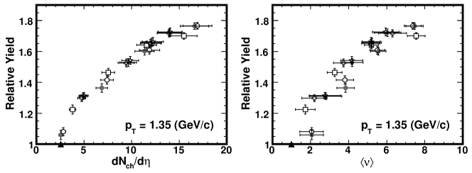
Figure 17: The average yield of hadrons having $p_{\mathrm{T}}=1.35~{}\mbox{\rm GeV$\kern-1.49994pt/\kern-1.19995ptc$}$ from d+Au collisions relative to p+p̄ as a function of both $d\!N_{\mathrm{ch}}/\mathit{d\eta}$ and $\left<\nu\right>$. Vertical error bars represent statistical uncertainties in the relative yield. Horizontal error bars represent systematic uncertainties (90% C.L.) in either $d\!N_{\mathrm{ch}}/\mathit{d\eta}$ or $\left<\nu\right>$.

See Fig. 16 for a description of the symbols.

Nevertheless, the data presented in Fig. 16 show two intriguing properties. One is that the relative yield of d+Au collisions is observed to extrapolate smoothly to the p+p̄ yield as the d+Au collisions become more peripheral. Thus, distortions of d+Au spectra caused by nuclear effects diminish in a smooth way as the amount of nuclear material probed by the deuteron is reduced. The other is that this centrality dependence of the shape of the d+Au spectra does not seem to depend on the choice of centrality measure, when the centrality of the collisions are parametrized by their integrated yield. This can be more easily seen in Fig. 17, which shows a detailed comparison of the relative yield as a function of both $d\!N_{\mathrm{ch}}/\mathit{d\eta}$ and $\left<\nu\right>$, at $p_{\mathrm{T}}=1.35~{}\mbox{\rm GeV$\kern-1.49994pt/\kern-1.19995ptc$}$. Vertical error bars represent statistical uncertainties, and therefore points could shift vertically independently. However, the horizontal error bars shown in this figure represent systematic uncertainties, and are expected to be highly correlated between different centrality measures (so the points would shift together in the horizontal direction). From this comparison, it is clear that the relative yield of d+Au extrapolates back to p+p̄ more smoothly when parametrized by the measured integrated yield.

Thus, such model independent parameterizations of centrality may provide the most unbiased, and therefore best, method with which to study the centrality dependence of hadron production in nucleon-nucleus and nucleus-nucleus system. Further, the common dependence of the relative yield on the mid-rapidity multiplicity among different centrality measures suggests that the outgoing particle density may play an important role in the Cronin effect. This observation provides additional evidence that the enhancement may be better described by models that consider final state effects, rather than initial partonic scattering only.

4 Comparison of p+Au and n+Au

The availability of both p+Au and n+Au collision data presented a unique opportunity to study baryon transport in nucleon-nucleus collisions. Since a p+Au collision contains one more charge than an n+Au collision, a search for this extra charge near the mid-rapidity region was possible. Previous measurements [152] of p+Au collisions at $\sqrt{s_{\scriptscriptstyle{{\rm NN}}}}=19.4~{}\mbox{${\rm GeV}$}$ found that the number of net protons (p - p̄) per unit of rapidity was less than one in the region of mid-rapidity. In addition, studies have shown a decrease in the mid-rapidity net proton yield with increasing center of mass energy; see [153] for a discussion. Further, it has been observed that hadrons traversing nuclear material do not lose more than about two units of rapidity [154]. Thus, it was expected that any charge asymmetry between hadrons measured at mid-rapidity in p+Au and n+Au collisions would be small.

Nevertheless, a comparison of charged hadron production in p+Au and n+Au allowed the transport of charge from the projectile proton, and from the projectile proton only, to be studied. Assuming that baryons from the gold nucleus underwent transport to mid-rapidity by the same process in p+Au and n+Au collisions, excess charge at mid-rapidity due to protons in the gold nucleus would not play a role.

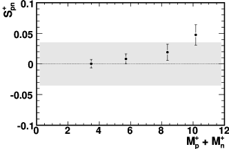
(a) $S_{pn}^{+}$

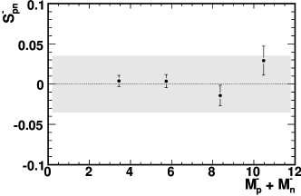
(b) $S_{pn}^{-}$

Figure 18: The asymmetry of charged hadrons in p+Au and n+Au collisions at $\left<\smash[b]{\eta}\right>=0.8$ as a function of centrality. The grey band shows the systematic uncertainty (90% C.L.) in the overal scale of the ratio. 18(a) The relative difference of positive hadron production between p+Au and n+Au collisions. 18(b) The relative difference of negative hadron production between p+Au and n+Au collisions.

Simple charge conservation would imply that the total number of positive particles emerging from a p+Au collision should be greater (by one) than the number emerging from a n+Au collision. Whether this charge asymmetry would be present near mid-rapidity was studied using the following observable.

$$S_{pn}^{+}=\frac{M_{p}^{+}-M_{n}^{+}}{M_{p}^{+}+M_{n}^{+}}$$ (6)

where $M_{p}^{+}$ denotes the integrated yield, $d\!N/\mathit{d\eta}$, of positive hadrons in p+Au collisions. The notation used for negative hadrons and n+Au collisions should be obvious.

The charge asymmetry defined by Eq. 6 is presented in Fig. 18 for both positive and negative hadrons. The grey band in each figure represents the systematic uncertainty in the asymmetry ratio due to uncertainties in the measured integrated yield. Only uncertainties specific to reconstructing the nucleon-nucleus $p_{\mathrm{T}}$ spectra (see Fig. 13(f)) contribute to this systematic error, as all other effects divide out in the ratio. No significant asymmetry between p+Au and n+Au collisions is observed at $\left<\smash[b]{\eta}\right>=0.8$, which is slightly forward on the deuteron side. However, the possibility for a similar measurement to be done using particles produced in more forward pseudorapidity regions is an exciting one. Such a study may be possible using the PHOBOS data and a particle tracking procedure that makes use of the inner-wing of the Spectrometer (see Sect. 2).

Chapter 8 Summary

The dynamics of strongly interacting matter under extreme conditions has been studied experimentally by the PHOBOS experiment. It was previously reported that the yield of charged hadrons with large transverse momenta in central Au+Au collisions at $\sqrt{s_{\scriptscriptstyle{{\rm NN}}}}=200~{}\mbox{${\rm GeV}$}$ is highly suppressed with respect to binary collision scaling [127, 128, 129, 130]. Two interpretations of this observation were proposed. The first suggested that the initial state of the nucleons in the nuclei were altered such that the production of high-$p_{\mathrm{T}}$ particles occurred less often in nucleus-nucleus collisions than in nucleon-nucleon interactions [132]. The second hypothesis held that the production of high-$p_{\mathrm{T}}$ particles was unaltered, but that the particles lost momentum due to subsequent interactions with a dense, strongly interacting medium [133]. These theories could be tested using nucleon-nucleus interactions, in which any nuclear effects, such as the modification of the initial nuclei, would be present, but a dense medium would not be produced. Due to technical considerations, the RHIC facility provided d+Au collisions to serve as the valuable control experiment. This decision involved two assumptions: firstly that differences between a d+Au and a nucleon-nucleus interaction were due only to the increased number of binary collisions, and secondly that the difference in the neutron content of the “projectile” in Au+Au, d+Au and p+p̄ interactions was unimportant.

The validity of these assumptions was tested by the analysis presented in this thesis. Detectors were added to the PHOBOS experiment that measured the energy of very forward-going single protons; both on the gold and deuteron exit side of the interaction region. The latter detector was used in conjunction with the ZDC detector to select d+Au collisions in which only the proton or neutron of the deuteron had interacted. Thus, samples of p+Au and n+Au collisions at $\sqrt{s_{\scriptscriptstyle{{\rm NN}}}}=200~{}\mbox{${\rm GeV}$}$ were obtained. Comparisons of the charged hadron yield in d+Au and p+Au collisions were used to validate the assumption of binary collision scaling from p+Au to d+Au. Further, an ideal nuclear modification reference for Au+Au collisions was constructed using a weighted combination of the yields in p+Au and n+Au interactions. This data verified that no bias was introduced through the use of a deuteron projectile rather than a nucleon projectile. In addition, it supported the conclusion that the large suppression of high-$p_{\mathrm{T}}$ hadron yields seen in Au+Au interactions are not observed in nucleon-nucleus collisions at $\sqrt{s_{\scriptscriptstyle{{\rm NN}}}}=200~{}\mbox{${\rm GeV}$}$. Thus, this data disfavors a hypothesis involving some modification of the initial nuclei and proves that final state effects play a significant role in the suppression of high-$p_{\mathrm{T}}$ hadrons in nucleus-nucleus collisions.

Further, a comparison of the yield of positively and negatively charged hadrons in p+Au and n+Au collisions was conducted. This comparison facilitated a rather unique study of charge transport, in that any excess positive charge yielded by p+Au interactions could be attributed to the proton from the deuteron nucleus in the initial state. No significant asymmetry between the charged hadron yields in p+Au and n+Au was observed at $\left<\smash[b]{\eta}\right>=0.8$.

Studies of the centrality dependence of the charged hadron yield of d+Au collisions were also performed. A method of centrality determination using the proton calorimeter on the gold exit side of the interaction region was developed. In addition, the centrality of collisions was ascertained using variables related to the multiplicity in different regions of pseudorapidity. It was found that in small systems like d+Au, the choice of centrality variable can significantly impact the resulting measurement. Variables based on the multiplicity in the mid-rapidity region were found to bias measurements performed in the mid-rapidity region such that the average collision in the most central bin was more central than either the fractional cross section or the number of participants would suggest. It was found that the least biased centrality variable used in measurements at mid-rapidity was one based on the multiplicity in a forward region of pseudorapidity. The PCAL centrality variables, based on the amount of nuclear spectator material, were not expected to introduce any bias on measurements at mid-rapidity. However, due to the lack of reliable simulations of PCAL signals in d+Au collisions, attempts to quantify the centrality of EPCAL bins using multiplicity based variables were influenced by the biases of those variables.

The multiple centrality variables were also used to study the centrality dependence of the shape of the charged hadron spectra in d+Au collisions. The modification of the $p_{\mathrm{T}}$ spectrum of nucleon-nucleus interactions as compared to a naïve superposition of nucleon-nucleon collisions is known as the Cronin effect [145]. This effect is characterized by an enhancement in the production of hadrons having $p_{\mathrm{T}}\sim 2.5~{}\mbox{\rm GeV$\kern-1.49994pt/\kern-1.19995ptc$}$. The centrality dependence of this enhancement was studied in nucleus-nucleus interactions for several values of $p_{\mathrm{T}}$. One may expect that as the amount of nuclear material the deuteron interacts with is decreased, the shape of the d+Au spectrum should smoothly approach that of p+p̄. This behavior is indeed seen when the centrality of d+Au collisions are parameterized by the multiplicity measured near mid-rapidity. Further, the same smooth extrapolation to p+p̄ was observed for the spectra as measured by all centrality variables, in spite of whatever bias each centrality variable may have introduced. On the other hand, no such smooth scaling for all centrality variables was present when the centrality of d+Au collisions was parameterized by $N_{\rm coll}$ or $\nu$. This observation seems to suggest that the Cronin effect may be driven by the density of outgoing particles, in addition to the number of scatterings a nucleon suffers during the initial collision.

Chapter 9 Centrality Results

The centrality parameters, such as $N_{\rm part}$, obtained using the various centrality measures, such as ERing, are presented in the following tables.

d+Au unbiased $N_{\rm coll}$ with dAuSpectra event selection
		$\left<N_{\rm coll}\right>\pm\text{Sys. Err.}$
Variable	Simulation	70-100%	40-70%	20-40%	0-20%
EOct	HIJING	$2.56\pm 0.77$	$6.15\pm 0.74$	$10.14\pm 0.72$	$14.31\pm 0.87$
EOct	AMPT	$2.57\pm 0.77$	$6.18\pm 0.74$	$10.11\pm 0.72$	$14.14\pm 0.86$
ERing	AMPT	$2.00\pm 0.60$	$4.99\pm 0.60$	$9.43\pm 0.67$	$14.49\pm 0.88$
EPCAL (EOct)	HIJING	$4.10\pm 1.27$	$7.05\pm 1.02$	$9.36\pm 1.07$	$11.15\pm 1.50$
EPCAL (EOct)	AMPT	$4.05\pm 1.26$	$7.10\pm 1.02$	$9.32\pm 1.07$	$11.01\pm 1.48$
EPCAL (ERing)	AMPT	$2.95\pm 0.92$	$6.15\pm 0.89$	$9.29\pm 1.06$	$11.77\pm 1.58$

Table 1: d+Au unbiased $N_{\rm coll}$ obtained using different centrality measures and the dAuSpectra event selection.

p+Au unbiased $N_{\rm coll}$ with dAuSpectra event selection
		$\left<N_{\rm coll}\right>\pm\text{Sys. Err.}$
Variable	Simulation	70-100%	40-70%	20-40%	0-20%
EOct	HIJING	$2.03\pm 0.61$	$4.29\pm 0.52$	$6.57\pm 0.47$	$8.25\pm 0.50$
EOct	AMPT	$2.01\pm 0.60$	$4.17\pm 0.50$	$6.30\pm 0.45$	$7.87\pm 0.48$
ERing	AMPT	$1.71\pm 0.51$	$3.70\pm 0.44$	$6.72\pm 0.48$	$8.36\pm 0.51$
EPCAL (EOct)	HIJING	$2.42\pm 0.73$	$3.18\pm 0.94$	$3.82\pm 1.10$	$4.41\pm 1.14$
EPCAL (EOct)	AMPT	$2.34\pm 0.70$	$3.06\pm 0.90$	$3.65\pm 1.05$	$4.18\pm 1.08$
EPCAL (ERing)	AMPT	$1.98\pm 0.59$	$2.87\pm 0.85$	$3.83\pm 1.11$	$4.83\pm 1.24$

Table 2: p+Au unbiased $N_{\rm coll}$ obtained using different centrality measures and the dAuSpectra event selection.

n+Au unbiased $N_{\rm coll}$ with dAuSpectra event selection
		$\left<N_{\rm coll}\right>\pm\text{Sys. Err.}$
Variable	Simulation	70-100%	40-70%	20-40%	0-20%
EOct	HIJING	$2.04\pm 0.61$	$4.29\pm 0.51$	$6.62\pm 0.47$	$8.23\pm 0.50$
EOct	AMPT	$2.02\pm 0.61$	$4.18\pm 0.50$	$6.33\pm 0.45$	$7.86\pm 0.48$
ERing	AMPT	$1.70\pm 0.51$	$3.73\pm 0.45$	$6.75\pm 0.48$	$8.36\pm 0.51$
EPCAL (EOct)	HIJING	$2.41\pm 0.73$	$3.17\pm 0.94$	$3.79\pm 1.17$	$4.39\pm 1.22$
EPCAL (EOct)	AMPT	$2.34\pm 0.70$	$3.06\pm 0.91$	$3.63\pm 1.12$	$4.18\pm 1.16$
EPCAL (ERing)	AMPT	$1.96\pm 0.59$	$2.85\pm 0.84$	$3.82\pm 1.18$	$4.82\pm 1.33$

Table 3: n+Au unbiased $N_{\rm coll}$ obtained using different centrality measures and the dAuSpectra event selection.

d+Au unbiased $N_{\rm part}$ with dAuSpectra event selection
		$\left<N_{\rm part}\right>\pm\text{Sys. Err.}$
Variable	Simulation	70-100%	40-70%	20-40%	0-20%
EOct	HIJING	$3.73\pm 0.84$	$7.48\pm 0.83$	$11.32\pm 0.94$	$15.15\pm 1.08$
EOct	AMPT	$3.75\pm 0.84$	$7.52\pm 0.83$	$11.28\pm 0.94$	$15.02\pm 1.07$
ERing	AMPT	$3.12\pm 0.70$	$6.31\pm 0.70$	$10.62\pm 0.88$	$15.42\pm 1.09$
EPCAL (EOct)	HIJING	$5.31\pm 1.22$	$8.25\pm 1.13$	$10.49\pm 1.21$	$12.19\pm 1.30$
EPCAL (EOct)	AMPT	$5.26\pm 1.21$	$8.30\pm 1.14$	$10.46\pm 1.21$	$12.07\pm 1.29$
EPCAL (ERing)	AMPT	$4.12\pm 0.94$	$7.36\pm 1.01$	$10.43\pm 1.20$	$12.82\pm 1.37$

Table 4: d+Au unbiased $N_{\rm part}$ obtained using different centrality measures and the dAuSpectra event selection.

p+Au unbiased $N_{\rm part}$ with dAuSpectra event selection
		$\left<N_{\rm part}\right>\pm\text{Sys. Err.}$
Variable	Simulation	70-100%	40-70%	20-40%	0-20%
EOct	HIJING	$3.03\pm 0.68$	$5.29\pm 0.59$	$7.57\pm 0.63$	$9.25\pm 0.66$
EOct	AMPT	$3.01\pm 0.67$	$5.17\pm 0.57$	$7.30\pm 0.61$	$8.87\pm 0.63$
ERing	AMPT	$2.71\pm 0.61$	$4.70\pm 0.52$	$7.72\pm 0.64$	$9.36\pm 0.66$
EPCAL (EOct)	HIJING	$3.42\pm 0.77$	$4.18\pm 1.03$	$4.82\pm 1.31$	$5.41\pm 1.25$
EPCAL (EOct)	AMPT	$3.34\pm 0.75$	$4.06\pm 1.00$	$4.65\pm 1.27$	$5.18\pm 1.20$
EPCAL (ERing)	AMPT	$2.98\pm 0.67$	$3.87\pm 0.95$	$4.83\pm 1.32$	$5.83\pm 1.35$

Table 5: p+Au unbiased $N_{\rm part}$ obtained using different centrality measures and the dAuSpectra event selection.

n+Au unbiased $N_{\rm part}$ with dAuSpectra event selection
		$\left<N_{\rm part}\right>\pm\text{Sys. Err.}$
Variable	Simulation	70-100%	40-70%	20-40%	0-20%
EOct	HIJING	$3.04\pm 0.68$	$5.29\pm 0.59$	$7.62\pm 0.63$	$9.23\pm 0.66$
EOct	AMPT	$3.02\pm 0.68$	$5.18\pm 0.58$	$7.33\pm 0.61$	$8.86\pm 0.63$
ERing	AMPT	$2.70\pm 0.61$	$4.73\pm 0.53$	$7.75\pm 0.64$	$9.36\pm 0.66$
EPCAL (EOct)	HIJING	$3.41\pm 0.77$	$4.17\pm 1.03$	$4.79\pm 1.31$	$5.39\pm 1.25$
EPCAL (EOct)	AMPT	$3.34\pm 0.75$	$4.06\pm 1.00$	$4.63\pm 1.26$	$5.18\pm 1.20$
EPCAL (ERing)	AMPT	$2.96\pm 0.67$	$3.85\pm 0.95$	$4.82\pm 1.31$	$5.82\pm 1.34$

Table 6: n+Au unbiased $N_{\rm part}$ obtained using different centrality measures and the dAuSpectra event selection.

d+Au unbiased $N_{\rm part}^{Au}$ with dAuSpectra event selection
		$\left<N_{\rm part}^{Au}\right>\pm\text{Sys. Err.}$
Variable	Simulation	70-100%	40-70%	20-40%	0-20%
EOct	HIJING	$2.44\pm 0.63$	$5.75\pm 0.75$	$9.40\pm 0.74$	$13.16\pm 0.97$
EOct	AMPT	$2.45\pm 0.64$	$5.77\pm 0.75$	$9.35\pm 0.74$	$13.03\pm 0.96$
ERing	AMPT	$1.92\pm 0.50$	$4.64\pm 0.60$	$8.70\pm 0.69$	$13.43\pm 0.99$
EPCAL (EOct)	HIJING	$3.86\pm 1.03$	$6.56\pm 1.04$	$8.67\pm 1.04$	$10.29\pm 1.36$
EPCAL (EOct)	AMPT	$3.81\pm 1.02$	$6.60\pm 1.04$	$8.64\pm 1.03$	$10.17\pm 1.35$
EPCAL (ERing)	AMPT	$2.79\pm 0.74$	$5.71\pm 0.90$	$8.60\pm 1.03$	$10.90\pm 1.45$

Table 7: d+Au unbiased $N_{\rm part}^{Au}$ obtained using different centrality measures and the dAuSpectra event selection.

p+Au unbiased $N_{\rm part}^{Au}$ with dAuSpectra event selection
		$\left<N_{\rm part}^{Au}\right>\pm\text{Sys. Err.}$
Variable	Simulation	70-100%	40-70%	20-40%	0-20%
EOct	HIJING	$2.03\pm 0.53$	$4.29\pm 0.56$	$6.57\pm 0.52$	$8.25\pm 0.61$
EOct	AMPT	$2.01\pm 0.52$	$4.17\pm 0.54$	$6.30\pm 0.50$	$7.87\pm 0.58$
ERing	AMPT	$1.71\pm 0.44$	$3.70\pm 0.48$	$6.72\pm 0.53$	$8.36\pm 0.62$
EPCAL (EOct)	HIJING	$2.42\pm 0.63$	$3.18\pm 0.98$	$3.82\pm 1.15$	$4.41\pm 1.15$
EPCAL (EOct)	AMPT	$2.34\pm 0.61$	$3.06\pm 0.94$	$3.65\pm 1.10$	$4.18\pm 1.09$
EPCAL (ERing)	AMPT	$1.98\pm 0.51$	$2.87\pm 0.89$	$3.83\pm 1.15$	$4.83\pm 1.26$

Table 8: p+Au unbiased $N_{\rm part}^{Au}$ obtained using different centrality measures and the dAuSpectra event selection.

n+Au unbiased $N_{\rm part}^{Au}$ with dAuSpectra event selection
		$\left<N_{\rm part}^{Au}\right>\pm\text{Sys. Err.}$
Variable	Simulation	70-100%	40-70%	20-40%	0-20%
EOct	HIJING	$2.04\pm 0.53$	$4.29\pm 0.56$	$6.62\pm 0.52$	$8.23\pm 0.61$
EOct	AMPT	$2.02\pm 0.53$	$4.18\pm 0.54$	$6.33\pm 0.50$	$7.86\pm 0.58$
ERing	AMPT	$1.70\pm 0.44$	$3.73\pm 0.49$	$6.75\pm 0.53$	$8.36\pm 0.62$
EPCAL (EOct)	HIJING	$2.41\pm 0.63$	$3.17\pm 0.98$	$3.79\pm 1.18$	$4.39\pm 1.23$
EPCAL (EOct)	AMPT	$2.34\pm 0.61$	$3.06\pm 0.95$	$3.63\pm 1.13$	$4.18\pm 1.17$
EPCAL (ERing)	AMPT	$1.96\pm 0.51$	$2.85\pm 0.88$	$3.82\pm 1.18$	$4.82\pm 1.35$

Table 9: n+Au unbiased $N_{\rm part}^{Au}$ obtained using different centrality measures and the dAuSpectra event selection.

d+Au unbiased $N_{\rm part}^{d}$ with dAuSpectra event selection
		$\left<N_{\rm part}^{d}\right>\pm\text{Sys. Err.}$
Variable	Simulation	70-100%	40-70%	20-40%	0-20%
EOct	HIJING	$1.29\pm 0.22$	$1.73\pm 0.21$	$1.92\pm 0.10$	$1.98\pm 0.11$
EOct	AMPT	$1.30\pm 0.22$	$1.74\pm 0.21$	$1.93\pm 0.10$	$1.99\pm 0.11$
ERing	AMPT	$1.20\pm 0.20$	$1.67\pm 0.20$	$1.93\pm 0.10$	$1.99\pm 0.11$
EPCAL (EOct)	HIJING	$1.45\pm 0.24$	$1.68\pm 0.23$	$1.82\pm 0.12$	$1.89\pm 0.11$
EPCAL (EOct)	AMPT	$1.45\pm 0.24$	$1.70\pm 0.23$	$1.82\pm 0.12$	$1.90\pm 0.11$
EPCAL (ERing)	AMPT	$1.33\pm 0.22$	$1.65\pm 0.22$	$1.83\pm 0.12$	$1.92\pm 0.11$

Table 10: d+Au unbiased $N_{\rm part}^{d}$ obtained using different centrality measures and the dAuSpectra event selection.

p+Au unbiased $N_{\rm part}^{d}$ with dAuSpectra event selection
		$\left<N_{\rm part}^{d}\right>\pm\text{Sys. Err.}$
Variable	Simulation	70-100%	40-70%	20-40%	0-20%
EOct	HIJING	$1.00\pm 0.17$	$1.00\pm 0.12$	$1.00\pm 0.05$	$1.00\pm 0.05$
EOct	AMPT	$1.00\pm 0.17$	$1.00\pm 0.12$	$1.00\pm 0.05$	$1.00\pm 0.05$
ERing	AMPT	$1.00\pm 0.17$	$1.00\pm 0.12$	$1.00\pm 0.05$	$1.00\pm 0.05$
EPCAL (EOct)	HIJING	$1.00\pm 0.17$	$1.00\pm 0.12$	$1.00\pm 0.05$	$1.00\pm 0.05$
EPCAL (EOct)	AMPT	$1.00\pm 0.17$	$1.00\pm 0.12$	$1.00\pm 0.05$	$1.00\pm 0.05$
EPCAL (ERing)	AMPT	$1.00\pm 0.17$	$1.00\pm 0.12$	$1.00\pm 0.05$	$1.00\pm 0.05$

Table 11: p+Au unbiased $N_{\rm part}^{d}$ obtained using different centrality measures and the dAuSpectra event selection.

n+Au unbiased $N_{\rm part}^{d}$ with dAuSpectra event selection
		$\left<N_{\rm part}^{d}\right>\pm\text{Sys. Err.}$
Variable	Simulation	70-100%	40-70%	20-40%	0-20%
EOct	HIJING	$1.00\pm 0.17$	$1.00\pm 0.12$	$1.00\pm 0.05$	$1.00\pm 0.05$
EOct	AMPT	$1.00\pm 0.17$	$1.00\pm 0.12$	$1.00\pm 0.05$	$1.00\pm 0.05$
ERing	AMPT	$1.00\pm 0.17$	$1.00\pm 0.12$	$1.00\pm 0.05$	$1.00\pm 0.05$
EPCAL (EOct)	HIJING	$1.00\pm 0.17$	$1.00\pm 0.12$	$1.00\pm 0.05$	$1.00\pm 0.05$
EPCAL (EOct)	AMPT	$1.00\pm 0.17$	$1.00\pm 0.12$	$1.00\pm 0.05$	$1.00\pm 0.05$
EPCAL (ERing)	AMPT	$1.00\pm 0.17$	$1.00\pm 0.12$	$1.00\pm 0.05$	$1.00\pm 0.05$

Table 12: n+Au unbiased $N_{\rm part}^{d}$ obtained using different centrality measures and the dAuSpectra event selection.

d+Au unbiased $\nu$ with dAuSpectra event selection
		$\left<\nu\right>\pm\text{Sys. Err.}$
Variable	Simulation	70-100%	40-70%	20-40%	0-20%
EOct	HIJING	$2.06\pm 0.62$	$3.84\pm 0.46$	$5.56\pm 0.39$	$7.47\pm 0.46$
EOct	AMPT	$2.06\pm 0.62$	$3.80\pm 0.46$	$5.51\pm 0.39$	$7.37\pm 0.45$
ERing	AMPT	$1.73\pm 0.52$	$3.27\pm 0.39$	$5.20\pm 0.37$	$7.55\pm 0.46$
EPCAL (EOct)	HIJING	$2.80\pm 0.84$	$4.18\pm 0.58$	$5.23\pm 0.49$	$6.04\pm 0.71$
EPCAL (EOct)	AMPT	$2.75\pm 0.83$	$4.17\pm 0.58$	$5.19\pm 0.48$	$5.95\pm 0.70$
EPCAL (ERing)	AMPT	$2.20\pm 0.66$	$3.73\pm 0.52$	$5.17\pm 0.48$	$6.30\pm 0.74$

Table 13: d+Au unbiased $\nu$ obtained using different centrality measures and the dAuSpectra event selection.

p+Au unbiased $\nu$ with dAuSpectra event selection
		$\left<\nu\right>\pm\text{Sys. Err.}$
Variable	Simulation	70-100%	40-70%	20-40%	0-20%
EOct	HIJING	$2.03\pm 0.61$	$4.29\pm 0.52$	$6.57\pm 0.47$	$8.25\pm 0.50$
EOct	AMPT	$2.01\pm 0.60$	$4.17\pm 0.50$	$6.30\pm 0.45$	$7.87\pm 0.48$
ERing	AMPT	$1.71\pm 0.51$	$3.70\pm 0.44$	$6.72\pm 0.48$	$8.36\pm 0.51$
EPCAL (EOct)	HIJING	$2.42\pm 0.73$	$3.18\pm 0.94$	$3.82\pm 1.10$	$4.41\pm 1.14$
EPCAL (EOct)	AMPT	$2.34\pm 0.70$	$3.06\pm 0.90$	$3.65\pm 1.05$	$4.18\pm 1.08$
EPCAL (ERing)	AMPT	$1.98\pm 0.59$	$2.87\pm 0.85$	$3.83\pm 1.11$	$4.83\pm 1.24$

Table 14: p+Au unbiased $\nu$ obtained using different centrality measures and the dAuSpectra event selection.

n+Au unbiased $\nu$ with dAuSpectra event selection
		$\left<\nu\right>\pm\text{Sys. Err.}$
Variable	Simulation	70-100%	40-70%	20-40%	0-20%
EOct	HIJING	$2.04\pm 0.61$	$4.29\pm 0.51$	$6.62\pm 0.47$	$8.23\pm 0.50$
EOct	AMPT	$2.02\pm 0.61$	$4.18\pm 0.50$	$6.33\pm 0.45$	$7.86\pm 0.48$
ERing	AMPT	$1.70\pm 0.51$	$3.73\pm 0.45$	$6.75\pm 0.48$	$8.36\pm 0.51$
EPCAL (EOct)	HIJING	$2.41\pm 0.73$	$3.17\pm 0.94$	$3.79\pm 1.17$	$4.39\pm 1.26$
EPCAL (EOct)	AMPT	$2.34\pm 0.71$	$3.06\pm 0.91$	$3.63\pm 1.12$	$4.18\pm 1.20$
EPCAL (ERing)	AMPT	$1.96\pm 0.59$	$2.85\pm 0.84$	$3.82\pm 1.18$	$4.82\pm 1.38$

Table 15: n+Au unbiased $\nu$ obtained using different centrality measures and the dAuSpectra event selection.

d+Au unbiased $b$ with dAuSpectra event selection
		$\left<b\right>\pm\text{Sys. Err.}$
Variable	Simulation	70-100%	40-70%	20-40%	0-20%
EOct	HIJING	$7.56$	$5.89$	$4.50$	$3.45$
EOct	AMPT	$7.43$	$5.81$	$4.49$	$3.47$
ERing	AMPT	$7.76$	$6.29$	$4.67$	$3.31$
EPCAL (EOct)	HIJING	$6.89$	$5.74$	$4.93$	$4.37$
EPCAL (EOct)	AMPT	$6.82$	$5.65$	$4.90$	$4.37$
EPCAL (ERing)	AMPT	$7.31$	$5.99$	$4.88$	$4.12$

Table 16: d+Au unbiased $b$ obtained using different centrality measures and the dAuSpectra event selection.

p+Au unbiased $b$ with dAuSpectra event selection
		$\left<b\right>\pm\text{Sys. Err.}$
Variable	Simulation	70-100%	40-70%	20-40%	0-20%
EOct	HIJING	$7.97$	$7.13$	$6.54$	$6.24$
EOct	AMPT	$7.85$	$7.06$	$6.53$	$6.21$
ERing	AMPT	$8.01$	$7.18$	$6.38$	$6.09$
EPCAL (EOct)	HIJING	$7.83$	$7.56$	$7.35$	$7.17$
EPCAL (EOct)	AMPT	$7.74$	$7.48$	$7.29$	$7.12$
EPCAL (ERing)	AMPT	$7.90$	$7.55$	$7.23$	$6.93$

Table 17: p+Au unbiased $b$ obtained using different centrality measures and the dAuSpectra event selection.

n+Au unbiased $b$ with dAuSpectra event selection
		$\left<b\right>\pm\text{Sys. Err.}$
Variable	Simulation	70-100%	40-70%	20-40%	0-20%
EOct	HIJING	$7.96$	$7.14$	$6.54$	$6.24$
EOct	AMPT	$7.84$	$7.05$	$6.51$	$6.24$
ERing	AMPT	$7.99$	$7.17$	$6.36$	$6.09$
EPCAL (EOct)	HIJING	$7.83$	$7.57$	$7.36$	$7.18$
EPCAL (EOct)	AMPT	$7.73$	$7.47$	$7.29$	$7.12$
EPCAL (ERing)	AMPT	$7.89$	$7.55$	$7.23$	$6.93$

Table 18: n+Au unbiased $b$ obtained using different centrality measures and the dAuSpectra event selection.

Chapter 10 Spectra Results

The invariant yield of positive, negative and average charged hadrons are presented in the following figures as a function of centrality, in four centrality bins as determined by six different centrality measures, for d+Au, p+Au and n+Au interactions.

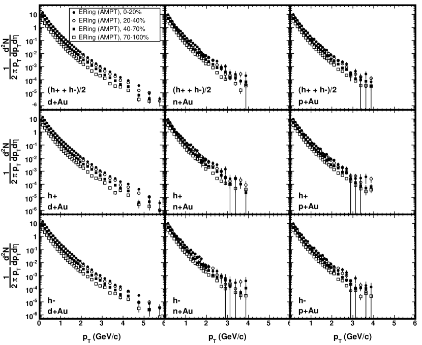
Figure 1: The invariant yield of $(\mathrm{h}^{+}+\mathrm{h}^{-})/2$, $\mathrm{h}^{+}$ and $\mathrm{h}^{-}$ in four centrality bins determined using AMPT and the ERing centrality variable. The spectra for d+Au, n+Au and p+Au are shown in separate columns. Only statistical errors are shown.

Figure 2: The invariant yield of $(\mathrm{h}^{+}+\mathrm{h}^{-})/2$, $\mathrm{h}^{+}$ and $\mathrm{h}^{-}$ in four centrality bins determined using HIJING and the EOct centrality variable. The spectra for d+Au, n+Au and p+Au are shown in separate columns. Only statistical errors are shown.

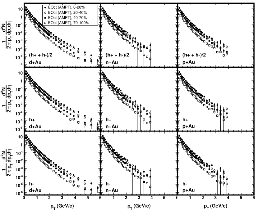
Figure 3: The invariant yield of $(\mathrm{h}^{+}+\mathrm{h}^{-})/2$, $\mathrm{h}^{+}$ and $\mathrm{h}^{-}$ in four centrality bins determined using AMPT and the EOct centrality variable. The spectra for d+Au, n+Au and p+Au are shown in separate columns. Only statistical errors are shown.

Figure 4: The invariant yield of $(\mathrm{h}^{+}+\mathrm{h}^{-})/2$, $\mathrm{h}^{+}$ and $\mathrm{h}^{-}$ in four centrality bins determined using AMPT and the EPCAL centrality variable. The trigger efficiency as a function of EPCAL was determined using ERing. The spectra for d+Au, n+Au and p+Au are shown in separate columns. Only statistical errors are shown.

Figure 6: The invariant yield of $(\mathrm{h}^{+}+\mathrm{h}^{-})/2$, $\mathrm{h}^{+}$ and $\mathrm{h}^{-}$ in four centrality bins determined using AMPT and the EPCAL centrality variable. The trigger efficiency as a function of EPCAL was determined using EOct. The spectra for d+Au, n+Au and p+Au are shown in separate columns. Only statistical errors are shown.

Chapter 11 Computing at PHOBOS

Major upgrades to the PHOBOS DAQ system prior to the d+Au physics run, and then again prior to the subsequent Au+Au run, greatly increased the amount of data that could be taken by the experiment. All told, the PHOBOS experiment had recorded around a billion collisions by the time the detector was decommissioned in June, 2005. The first data storage format developed by PHOBOS, and used for all its publications prior to 2006, was not suitable for efficient storage and access to such a large volume of data. In this format, data from an average reconstructed Au+Au collision (consisting of calibrated detector signals, reconstructed vertices and Spectrometer tracks) took up over 100 ${\rm kB}$ of storage space. Due to the size of collisions in this format, it was not possible to store all of the data in a location that was easily accessible by physicists. The need to store this data on the PHOBOS computer farm at RCF, where it could be repeatedly analyzed, led to two major software projects. The first was the development of a new, highly efficient data storage structure known as an Analysis Tree (AnT). The second was a new framework in which the TTree objects of An Object-Oriented Data Analysis Tool (ROOT) [155] (as well as AnTs) could be analyzed.

Appendix 11.A Analysis Trees in PHOBOS

The AnT format reduced the size of the average collision data by more than a factor of two, while also increasing the efficiency with which it could be processed. This was achieved by using the ROOT package’s TTree class as the backbone of the format. The TTree class was designed to provide improvements in data storage and processing efficiency over the standard ROOT file Input/Output (I/O).

Figure 1: A display of the contents of a PHOBOS data file prior to AnT, using TBrowser. The selected item is the MultBinInfo object of event number 1000, which contains the ERing value for the event.

The first PHOBOS data format consisted of various objects, such as hits and tracks, all contained in a single collision event container. Each event was independently written to a ROOT file, as illustrated in Fig. 1. The major disadvantage of this structure was the inefficiency of data access. For example, to generate an ERing distribution, it was necessary to (a) read an entire event from the file into memory, (b) locate the “MultBinInfo” object that stored ERing, (c) fill a histogram with the ERing value and (d) delete the event object. These four steps would then need to be repeated for each collision.

Figure 2: A display of the contents of an AnT file. The selected item is the ERing leaf of the centrality branch, which contains the ERing value of each event.

The AnT format improved this situation by storing objects in the branches of a TTree. A TTree can be pictured as a large table, the columns of which are buffers (branches) filled with data (leaves) and the rows of which correspond to entries in the tree. In the case of AnTs, each entry was a single collision event. This structure, illustrated in Fig. 2, had two main advantages. First, branches in the tree could be read independently. Thus, continuing the example above, to access the OctDe vertex information, only the branch containing vertices would need to be read (and not the entire event). This provided a major increase in processing speed; analyses that did not need to process raw Silicon hits ran an order of magnitude faster with the AnT data format. The second advantage was that data could be compressed far beyond that of a standard ROOT file. Because each entry in any particular branch stored data of the same type, there was no need to write out the same descriptive header information for every entry. With the standard ROOT I/O, the full object information (header included) would be written to the file for every object in every event. For more information on the TTree class, see [156].

An AnT was a ROOT file that contained one TTree. Each branch of this tree contained a part of the collision event data: raw Silicon hits, merged hits, reconstructed tracks, vertices, etc. New classes were created to store this data in the most efficient way possible. All data members of such a class were made public to increase the ease of access. The type of a data member was chosen so as to use the minimum number of bytes possible. For example, a merged hit stored the number of the Silicon layer in which it was located. Since this number could not be more than 255, as there were 16 Spectrometer layers, only one byte was used to store this information.

Disk space and processing efficiency was further improved through the use of TClonesArray [156]. A TClonesArray was a special container that stored multiple objects of the same class. Since each object in the container was of the same type, the memory for these objects was allocated only once. Thus, if a TClonesArray was used to store hits in an event, the first hit in every event would be read into the same memory space. On the other hand, with a standard collection class such as TObjArray, memory would be allocated (and de-allocated) each time a new event was read. The AnT format used TClonesArray objects extensively to store groups of related objects, such as the list of merged Spectrometer hits and the list of reconstructed tracks.

Appendix 11.B Parallel ROOT Facility

The Parallel ROOT Facility (PROOF) package was designed to allow the analysis of a large set of data in an efficient and interactive manner. This was achieved by parallelizing the reading and processing of data on a computing cluster with distributed storage. An analysis run under PROOF began at the user’s computer, referred to as the client. There, the set of data to be processed was specified, as were the cluster Central Processing Units, referred to as slaves, that would be used for processing. At the start of the analysis, a PROOF master was initialized. The master node coordinated the data processing by fulfilling each slave’s request for work. That is, idle slaves would ask the master for instruction on which data to process, and the master would send a packet of work in return. This ensured that faster slaves processed more data than slower slaves, and optimized disk I/O by allowing a slave to process local data whenever possible. Finally, after the slaves had completed processing, the results from each slave were collected and merged into a single result, which was then passed back to the client. Thus, PROOF allowed the user to exploit the advantages of parallel processing, without sacrificing the simplicity of a local, interactive ROOT analysis. For more information on PROOF, see [157].

Appendix 11.C Tree-Analysis Modules

To analyze data stored in the AnT format, a software package known as Tree-Analysis Modules (TAM) was developed. TAM provided the infrastructure for the processing of data stored in ROOT trees using modules. A module was a user-created object structured like a TSelector (see [156]), but which had certain advantages over the ROOT selector. As with a TSelector, a TAM module had the benefit of automated tree interaction (that is, the user did not have to explicitly call TBranch::SetAddress nor loop over entries) and it interfaced well with the PROOF package. However, modules were not subject to some of the drawbacks of selectors. Selectors were typically large monolithic macros, generated by TTree:MakeSelector, making them difficult to share with other users in a collaboration. These large macros also tended to result in users copying blocks of code in order to gain certain functionality. Both of these issues could be avoided by the use of TAM, which allowed users to separate parts of an analysis into different modules and allowed them to run other users’ modules as part of their own analysis. In addition, one of the main goals of TAM was to make running an analysis with PROOF transparent for the user; that is, one could process data with or without PROOF and not need to make any changes to a TAM module.

Class	Description
TAModule	The base class of all user-created modules.
TAMSelector	The manager. Scheduled the execution of modules and the interaction with the tree.
TAMOutput	An output container. Handled the merging of objects under PROOF.

Table 1: The classes in the TAM package.

The TAM package was designed around three main goals. First, to provide a very general, modular framework for analyzing data in ROOT trees. Second, to hide, as much as possible, all interaction with the tree itself from the user. Third, to ensure compatibility with PROOF and to make the use of PROOF transparent to the user. This led to the development of three classes: TAModule, the basis of all user-created modules, TAMSelector, which managed the modules and interaction with the tree, and TAMOutput, which managed the output of modules. These classes are summarized in Table 1.

1 Modules

An analysis in TAM was performed using a hierarchy of modules. That is, a module could have any number of submodules. This capability was provided by the base class of TAModule, TTask (see [156]). This feature allowed a module to control the processing of submodules, either through error handling (described in Sect. 1) or by directly accessing a submodule. It also allowed a user to package an analysis into a “supermodule,” a concept borrowed from the earlier PHOBOS analysis framework. A supermodule was a collection of modules that had been organized to produce some particular output, which could then be easily utilized by any user. For example, a supermodule could be constructed to determine the reaction plane of a collision. This supermodule would then be run by all users doing analyses that require knowledge of the reaction plane.

Function	Executed On	Description
Begin	Client	Startup code. Typically not used.
SlaveBegin	Slave	Startup code. Output (i.e. histograms) was initialized and branches were requested here.
Notify	Slave	Called when a new file was opened. Typically not used.
Process	Slave	Called during the event loop. Data was loaded and histograms were filled here.
SlaveTerminate	Slave	Finishing code. Typically not used.
Terminate	Client	Finishing code.

Table 2: Functions TAM package.

At its most basic, a module would perform its analysis by (a) making some histograms, (b) loading some data and (c) filling the histograms. This flow of execution was broken up into six functions, as shown in Table 2. The Begin function was called (by TAMSelector) first, and was used to run initializing code on the client computer. This function was not usually needed by a module. Next, the SlaveBegin function was called on the PROOF slave. This function was used to initialize any output, such as a histogram, and to request the branches that would be needed (see Sect. 1). Then the event loop would begin, as each entry of the tree was processed by TAM. The Notify function would be called on the slave whenever a new file had been opened. This function was not typically used by a module, but could in principal have been useful for loading calibrations or some other file-dependent information. The Process function was called on the slave for each entry of the tree. This was typically the most important function of a module, in which the data was loaded, some event selection was applied, analysis calculations were performed and histograms were filled. After all entries of the tree had been processed, the SlaveTerminate function was called on each slave, to perform any post-event-loop tasks that needed to be performed prior to the merging of output from each slave. This function was not typically used by a module. Finally, after the output of each PROOF slave had been merged (see Sect. 3), the Terminate function was called. This function was used to finish the analysis; for example fitting a function to the final distribution could have been done here.

Requesting Data

Modules did not directly retrieve data from the tree; rather, they instructed TAM to do so. This was done using two functions, RequestBranch and LoadBranch. The former function, called during SlaveBegin, was used to inform the TAMSelector that the module may use data from the specified branch. LoadBranch, called during Process, initiated the actual loading of data out of the tree. This structure was used to ensure efficient reading of the data. By forcing a user to load entries from the tree branch-by-branch, the user was encouraged to load only the minimal amount of data necessary for the current processing. That is, one would generally load some sort of event selection branch first, perform the selection, and then, if the current event passed the selection, load the remaining data.

The RequestBranch function was a templated function that took (a) the name of the branch being requested and (b) the pointer used by the module to access the data. The function was templated to allow TAM to check that the pointer type was appropriate for the data stored in the branch, as described in Sect. 2. The LoadBranch function took only the name of the branch. The actual loading of the data by TAMSelector is described in Sect. 2.

A typical PHOBOS module would load a branch that contained general information about an event, such as the event number in the file. A simple example of such a module follows. First, the module would declare the pointer it would use to access the data.

     class TExampleTAM : public TAModule {  private:     TPhAnTEventInfo*  fEvtInfo; // event info from the AnT     

While the pointer would eventually be made to point to the data by TAM, as will be described in Sect. 2, it would first be initialized to zero in the constructor.

     TExampleTAM::TExampleTAM(const Char_t* name,                           const Char_t* title) :     TAModule(name, title),     fEvtInfo(0) {  }     

The appropriate branch, named “eventInfo” in this example, would then be requested in SlaveBegin.

     void TExampleTAM::SlaveBegin() {     ReqBranch("eventInfo",fEvtInfo);  }     

Finally, in Process, the data could be loaded and used.

     void TExampleTAM::Process() {     LoadBranch("eventInfo");     Info("Process","This is event number [%d]",          fEvtInfo->fEventNum);  }     

Error Handling

Action Name	Description
kSuccess	Print a warning and continue processing.
kAbortModule	Print an error message and stop this module (and its submodules) from processing the current event.
kAbortEvent	Print an error message and stop all modules from processing the current event.
kAbortAnalysis	Print a break message and stop all modules from any further processing.

Table 3: The flow control options of SendError.

TAM provided some basic functionality for error handling via the SendError function. This function was similar to the TObject::Error and Warning functions, except that it granted modules the ability to control the flow of processing. There were four levels of flow control, summarized in Table 3.

The kSuccess option merely printed a warning. The flow of processing was not altered. The kAbortModule option printed an error message and stopped this module, and its submodules, from further processing of the current event. The module would return to its normal state at the next event. That is, if called during Process, the module would not be active for the current entry, but would return to normal when processing the next entry of the tree. If called during SlaveBegin, for example, then the module would return to normal for the first Notify or Process call (whichever came next). The kAbortEvent option printed an error message and stopped all modules from further processing of the current event. The modules would return to normal before processing the next event. Finally, the kAbortAnalysis option printed a break message and stopped all further processing of all modules. An example showing the usage of SendError follows.

     void TExampleTAM::Process() {     LoadBranch("eventInfo");     const Int_t num = fEvtInfo->fEventNum;     if (num > 100) {        SendError(kAbortModule,"Process",                  "Event number [%d] too big.",                  fEvtInfo->fEventNum);        return;     }  }     

While not useful for error handling, one other method of flow control available to modules was the SkipEvent function. This function controlled the flow of processing at the kAbortModule level, but did not print any error message. This was useful for allowing a module to implement an event selection and prevent submodules from processing rejected events.

Interacting With Other Modules

Often during an analysis, it would be useful for modules to access data that was not stored in the tree. Two distinct situations were typical: (a) data objects that were relevant only for the current entry in the tree and (b) more static data objects that were relevant throughout the analysis.

Objects relevant to the current entry of the tree could be made available to any module and would be properly disposed of before the processing of the next entry. This functionality was provided by the AddObjThisEvt function, which stored the object in THashList for fast-lookup (see [158] for a discussion of hash tables). Any module could then access the object using the FindObjThisEvt function. Such functionality would be useful, for example, if module $A$ produced some tracks from hits stored in the tree and module $B$ used those tracks to generate some momentum spectra. All objects passed to the AddObjThisEvt function would be automatically deleted by TAM before the processing of the next tree entry. If a module wanted to prevent this deletion, and deny other modules access to the object, the object could be removed from the event via the RemoveObjThisEvt function. Objects added to the event were required to have a unique name, such that the name could be hashed. For an object that did not inherit from TNamed, TAM would store the object under the class name.

For the more static data objects, a different interface was used. The PublishObj function was used to make an object available to all modules, all throughout the analysis. The FindPublicObj function could be used to access the public object. This functionality would be useful for supplying modules with some calibration objects, for example. Like objects added to the event, public objects were also required to have a unique name. This restriction was due to the fact that the PROOF input list was used to send such objects to the slave computers, and PROOF lists were name-based. Unlike objects added to the event, it was the user’s responsibility to clean up public objects. In order to prevent dangling pointer issues, it was important for the user to call the RetractObj function before deleting the object. This function would remove the object from the list of public objects.

Using PROOF

TAM was designed to make running an analysis with PROOF as simple as possible. One of the (somewhat superficial) ways in which this was accomplished was by making the syntax similar for analyses run with and without PROOF. While no change at all needed to be made to modules when running with PROOF, it was of course necessary to start the analysis in a different way.

An example analysis may be scripted as follows. First, the module hierarchy would be built.

     TMyTAMMod* myMod    = new TMyTAMMod;  TMySubMod* mySubMod = new TMySubMod;  myMod->Add(mySubMod);     

Then, for an analysis without PROOF, the modules would be added directly to the TAMSelector.

     TAMSelector* mySel = new TAMSelector;  mySel->AddInput(myMod);  tree->Process(mySel);  TList* output = mySel->GetModOutput();     

For an analysis using PROOF, the modules would be added to the TDset object and the output would be obtained from PROOF, rather than from the selector. However, the syntax was similar, as emphasized by the bold text.

     dset->AddInput(myMod);  dset->Process("TAMSelector");  TList* output = gProof->GetOutputList();     

This is essentially all that is required to run an analysis under TAM with PROOF. Other issues, such as porting the module hierarchy to the slaves and extracting their output (see Sect. 3), are handled by TAM.

2 The Selector

While TAModule enforced the structure of a module, most of the features of the TAM package were implemented in the TAMSelector class. The module hierarchy was maintained by the selector, using its own TAModule to store other modules. This top-most module did no processing and was merely a (hidden) container for the user’s modules. All of the module processing calls, such as SlaveBegin or Process, were called by the selector. Care was taken by the selector to ensure that the list of objects associated with the event was properly cleaned at the end of each process call, and that each module’s pointers to data were reset to zero before it could analyze the next entry of the tree (to prevent dangling pointers). Most of the interaction with the tree was handled by the nested class TAMSelector::TAMBranchInfo. This class was used to load the data of a requested class, set the modules’ pointer and to ensure data integrity. As described in Sect. 4, this nested class evolved into an extension to TAM that opened the door for users to control the loading of data from the tree (i.e. to allow for event mixing type analyses).

Loading Data

Type	Variable	Description
Bool_t	fIsLoaded	True if LoadBranch had already been called by some module for this branch.
Bool_t	fIsClass	True if this branch in the tree stored an object (as opposed to a list of numbers).
Bool_t	fLeafSizeConst	True if this branch stored a list of numbers that each used the same number of bytes.
TBranch*	fBranch	The branch object from the current tree.
void*	fBAddr	The memory location into which data from the tree would be read.
vector<BranchPtr_t*>	fUsrAddresses	List of pointers used by each module to access data from this branch. BranchPtr_t was templated to preserve the type of pointer used by each module.

Table 4: The information about each branch stored by
TAMSelector::TAMBranchInfo.

The loading of data from the tree was managed by TAMSelector. The selector stored a (hash) table of TAMSelector::TAMBranchInfo objects, each of which held information about a branch that had been requested by a module. The information stored about each branch is summarized in Table 4. This table was built up by the modules’ ReqBranch calls. Each time ReqBranch was called, a new entry in the table would be made if necessary, and the module’s pointer would be added to the list of pointers for that branch, fUsrAddresses. The name of each TAMBranchInfo object was simply the name of the branch in the tree, and this name was used for the hash lookups. Thus, whenever a module would call LoadBranch, TAMSelector would retrieve the TAMBranchInfo object for the specified branch. Then, if fIsLoaded was false, the data for the branch would be loaded through a simple fBranch->GetEntry call. Finally, the pointer for each module would be set to point to the data in memory and fIsLoaded would be set to true.

The memory address into which the branch was read depended on the type of data stored in the tree. For branches that stored (a) objects or (b) lists of numbers, each of which were the same size, a simple call to TTree::SetBranchAddress during Notify was made. However, a more complicated situation arose when the branch stored a list of numbers that were not all the same size. As discussed in the ROOT User’s Guide [156], the data would be read into memory as a simple array of numbers. Thus, for the branch

     *Br 0 :MyParticle : PID/S:Momentum[3]/F *     

14 bytes of data would be read from the tree. The first two bytes would be the particle identity, stored as a Short_t, and the next 12 bytes would be the three components of the momentum vector, each stored as a Float_t. The structure used to access this data by a modules would take the following form.

     struct MyParticle_t {     Short_t PID;     Float_t Momentum[3];  };     

Thus, in order to properly access the data, one would need to be sure that the start of the momentum array was only two bytes after the address of PID. However, C++ makes no such guarantee. A compiler could buffer the structure such that each variable would be evenly spaced in memory – that is, each variable would be 4 bytes apart. To prevent errors that would result in such a situation, TAM individually set the address of each leaf of the branch. This was done by exploiting the TDataMember class of ROOT, which gave the offset of each variable in the structure (that is, the number of bytes between a variable and the start of the structure). For TDataMember to have access to the make-up of the structure, it was necessary for the user to add the structure to the ROOT dictionary, in the usual way.

     #pragma link C++ class MyParticle_t+;     

Type Checking

To further ensure that the data being read from the tree was properly accessed by the modules, TAM implemented type checking. Type checking was run during Notify, prior to any data being loaded from the tree. For branches that stored an object, the type checking was simple. A loop over the list of module pointers, fUsrAddresses, was performed. The type of each pointer, as reported by type_info, was required to be the same as the type of the class stored in the branch.

For a branch that stored a list of numbers, the type checking was a bit more thorough. The list of leaves was obtained from the branch. Concurrently, the list of variables in the structure was obtained using TClass::GetListOfDataMembers. These lists were then looped over together. The type name of the leaf in the tree was required to be the same as the name of the variable type, as reported by TDataMember::GetTypeName. While this check was being performed, the size of each variable in the structure was also checked, such that the TAMBranchInfo::fLeafSizeConst variable could be set appropriately.

3 Output

The TAMOutput class was used to store the output of a module. This class was explicitly designed to make running TAM under PROOF transparent. It handled the merging of objects as they were returned from the PROOF slaves. It also attempted to associate a module’s pointers to its output objects with the merged objects in PROOF’s output list. This issue was important, since a module would create a histogram, for example, during SlaveBegin. Thus, the histogram would exist only on the slave computer. When the slaves finished processing, the histogram would be stored in the output list of PROOF and the module’s pointer to the histogram would be zero on the client. TAMOutput would automatically set the module’s pointer to point to the merged histogram.

Figure 3: Browsing the hierarchy of module output.

In addition, the TAMOutput class was browsable, as shown in Fig. 3. The browser allowed the user to visually navigate the module hierarchy. This was especially useful since output objects were retrieved using the FindOutput function, which required the user to know which module had produced the output. Thus, the browser was useful for locating output objects in a large module hierarchy.

Merging

TAM stored in the output list of PROOF the TAMOutput object of the top-most, hidden module. Thus, when the slave computers finished processing, PROOF would automatically call Merge on these TAMOutput objects (one for each slave). The module output objects contained both (a) a list of the output objects for its module and (b) a list of the TAMOutput objects associated with each submodule. This way, the module hierarchy was preserved in the output.

The first task performed by TAMOutput::Merge was to merge the output objects of the current module. This was done by looping over the corresponding TAMOutput objects from each slave. A list of objects to merge was then assembled. That is, the first output object from each slave was put into a list. Then, the objects in this list were merged. For example, the first output object from the first slave would be combined with the first output object from the second slave using the TObject::Merge function. Then, this combined object would be merged with the first output object from the third slave; and so on. The same would be repeated for the second output object from each slave, then the third, and so on. The final result would be a single TAMOutput class for the module whose list of output objects is filled with the combined results of each slave.

The next task was to properly merge the output of submodules, while preserving the module hierarchy. This was done by looping through the list of slaves and generating a list of the first submodule’s TAMOutput from each slave. This list of first submodules was then sent into TAMOutput::Merge. The procedure was then repeated for the second submodule from each slave, and so on. Note that because this loop over submodule output objects was contained in the TAMOutput::Merge function, the recursive behavior required to merge, for example, sub-submodule output, was obtained automatically. For example, the output of the first submodule (of the first module) would be merged before the output of the second module would be merged.

Extraction from PROOF Output List

A module stored an output object, such as a histogram, using the AddOutput function. Because modules created their output objects during SlaveBegin, there was an issue with modules running under PROOF trying to access these object directly. For example, suppose a module did the following. In SlaveBegin, some output object, a histogram, was created.

     void TExampleTAM::SlaveBegin() {     ReqBranch("eventInfo",fEvtInfo);     fEvtNum = new TH1F("hEvtNum","Event Numbers",100,0,100);  }     

Then, in Process, the histogram was filled.

     void TExampleTAM::Process() {     LoadBranch("eventInfo");     fEvtNum->Fill(fEvtInfo->fEventNum);  }     

Finally, in Terminate, the histogram was displayed.

     void TExampleTAM::Terminate() {     fEvtNum->Draw();  }     

This code would work if the module were run without PROOF. However, under PROOF, the module would crash during Terminate. The reason is simple: fEvtNum was created on the slave computer. On the client computer, fEvtNum would still be zero (shown in bold in the example above). The merged histogram would be sitting in the module’s list of output objects, and it would be up to the user to write special code when running under PROOF in order to extract the object from the output list.

TAM avoided this situation, and made running under PROOF transparent, by doing the work for the user, starting with AddOutput. This function stored both the output object as well as information about how the module accessed the output object. First, the output object itself was added to the list of output objects in the TAMOutput. Then, the address of the pointer (not the address the pointer pointed to) that was sent to AddOutput was checked against the address of each of the module’s member variables. If a match was found, then information about this variable was stored in a hash table. Because AddOutput was called during SlaveBegin on the slave computers, it was not necessary to store the address of the pointer (since this address would be different on the client computer). Instead, both the name of the member variable and the name of the output object were stored in the table. The name of the output object was used as the hash key for fast-lookup.

Finally, back on the client computer, each module’s member variables could be made to point to the appropriate (merged) output object. This was done by looping through the list of output objects. For a given output object, an attempt was made to find an entry in the member variable table that stored the name of the output object in question. If one could be found, then the name of the module’s member variable was retrieved from that entry of the table. Using the variable name, the TClass::GetDataMember function was called to access the appropriate member variable. This member variable was then explicitly set to point to the corresponding output object. Note that this method could only work when the variable passed to AddOutput was (a) a member variable of the module and (b) a pointer to an object – and not, say, the address of an instance. The former requirement was enforced implicitly, since entries in the lookup table could only be made for member variables. The latter requirement was explicitly enforced. The GetFullTypeName function of TDataMember was used to get the type of the module’s member variable as a string. This string was required to have the form Class*.

4 Data Loader Plug-ins

While the version of TAM described in this thesis provided a feature-rich environment in which users could process ROOT trees, it was not easily adapted to event-mixing type analyses. That is, this version of TAM assumed that the user was processing a single tree and that each entry could be processed independently. To accommodate analyses for which these assumptions are not valid, the concept of a data loading plug-in was developed. The goal was for users to have the ability to control the way in which data would be loaded. An analysis would still be driven by a single tree, but the user could control how the data would be read from the tree. For example, in an event mixing analysis, one might use certain properties of the current collision, such as the vertex location, to generate a mixed event from collisions in a second tree that have a similar vertex. Such a procedure could be coded by a user into the plug-in. TAM would then access data via this plug-in, rather than by the traditional TAMSelector::TAMBranchInfo class. Thus, the same module would be used to process a mixed event or a collision event; only the plug-in used to load the data would change. As of this writing, development of the plug-in extension to TAM is maturing rapidly, and preliminary versions are being tested.

Chapter 12 List of Acronyms

Facilities:

AGS

Alternating Gradient Synchrotron (http://www.bnl.gov/bnlweb/facilities/AGS.asp)

BNL

Brookhaven National Laboratory (http://www.bnl.gov/)

RCF

RHIC Computing Facility (http://www.rhic.bnl.gov/RCF/)

RHIC

Relativistic Heavy Ion Collider (http://www.bnl.gov/RHIC/)

PHOBOS Hardware:

ADC

Analog-to-Digital Converter

Au-PCAL

Proton Calorimeter on the Au-exit side

Au-ZDC

Zero-Degree Calorimeter on the Au-exit side

d-PCAL

Proton Calorimeter on the d-exit side

d-ZDC

Zero-Degree Calorimeter on the d-exit side

DAC

Digital-to-Analog Converter

DAQ

Data Acquisition

DRAM

Dynamic Random Access Memory

FEC

Front-End Controller

FPDP

Front Panel Data Port (http://www.fpdp.com/)

HPSS

High Performance Storage System (http://www.hpss-collaboration.org/hpss/index.jsp)

LED

Light-Emitting Diode

PCAL

Proton Calorimeter

PMT

Photomultiplier Tube

SpecTrig

Spectrometer Trigger

SRAM

Static Random Access Memory

T0

Time-Zero Counter

TDC

Time-to-Digital Converter

TOF

Time-of-Flight

VME

VERSAmodule Eurocard

ZDC

Zero-Degree Calorimeter

Experiment Terminology:

AA

nucleus-nucleus

AMPT

A Multi-Phase Transport

AnT

Analysis Tree

CMN

Common-Mode Noise

ART

A Relativistic Transport

CPU

Central Processing Unit

dAuMinBias

d+Au Minimum Bias

dAuPeriph

d+Au Peripheral

dAuSpectra

d+Au Spectra

dAuVertex

d+Au Vertex

EOct

Energy in Octagon

EPCAL

Energy in Au-PCAL

ERing

Energy in Rings

HIJING

Heavy Ion Jet Interaction Generator

I/O

Input/Output

IP

Nominal Interaction Point

IsCol

Is Collision

L0

Level 0

L1

Level 1

L2

Level 2

MC

Monte Carlo

NN

nucleon-nucleon

OctDe

Octagon Deposited Energy

PROOF

Parallel ROOT Facility

ROOT

An Object-Oriented Data Analysis Tool

SpecN

the inner-ring Spectrometer arm

SpecP

the outer-ring Spectrometer arm

TAM

Tree-Analysis Modules

TPC

Time Projection Chamber

ZPC

Zhang’s Parton Cascade

Mathematical Terminology:

RMS

Root-Mean-Square

Physics Terminology:

MIP

Minimum Ionizing Particle

ONO

Oxide-Nitride-Oxide

QCD

Quantum Chromodynamics

QGP

Quark-Gluon Plasma

References

- domain image [Macmillan and Company, 1914] Public domain image. Practical Physics, Macmillan and Company, 1914. Obtained from http://en.wikipedia.org/wiki/Image:Magnet0873.png.
- et al [2006a] W. M. Yao et al. Review of particle physics. J. Phys., G33:1–1232, 2006a.
- Cristinziani [2003] M. Cristinziani. Search for antimatter with the AMS cosmic ray detector. Nucl. Phys. Proc. Suppl., 114:275–279, 2003. [arXiv:astro-ph/0303641].
- Rolnick [1994] W. B. Rolnick. The Fundamental Particles and Their Interactions, chapter 15: Evidence for the Standard Model with Three Generations, pages 296–331. Addison-Wesley Pub. Co., Reading, Massachusetts, USA, 1994. ISBN 0-201-57838-7.
- Ashtekar and Lewandowski [2004] A. Ashtekar and J. Lewandowski. Background independent quantum gravity: A status report. Class. Quant. Grav., 21:R53, 2004. [arXiv:gr-qc/0404018].
- Escribano and Masso [1998] R. Escribano and E. Masso. High precision tests of QED and physics beyond the standard model. Eur. Phys. J., C4:139–143, 1998. [arXiv:hep-ph/9607218].
- Landau and Lifshitz [1958] L. D. Landau and E. M. Lifshitz. Quantum mechanics, chapter 11: The Diatomic Molecule. Addison-Wesley Pub. Co., Reading, Massachusetts, USA, 1958.
- Isgur [1985] N. Isgur. Nuclear physics from the quark model with chromodynamics. In M. B. Johnson and A. Picklesimer, editors, RELATIVISTIC DYNAMICS AND QUARK NUCLEAR PHYSICS. PROCEEDINGS, WORKSHOP, LOS ALAMOS, USA, pages 619–690, JUNE 1985. UTPT-85-18.
- Perkins [1987] D. H. Perkins. Introduction to High Energy Physics. Addison-Wesley Pub. Co., Reading, Massachusetts, USA, 1987. ISBN 0-201-12105-0.
- et al [1998a] M. Shiozawa et al. Search for proton decay via p –> e+ pi0 in a large water Cherenkov detector. Phys. Rev. Lett., 81:3319–3323, 1998a. [arXiv:hep-ex/9806014].
- Friedmann and Witten [2003] T. Friedmann and E. Witten. Unification scale, proton decay, and manifolds of G(2) holonomy. Adv. Theor. Math. Phys., 7:577–617, 2003. [arXiv:hep-th/0211269].
- Compagno et al. [1995] G. Compagno, G. M. Palma, R. Passante, and F. Persico. Atoms dressed and partially dressed by the zero-point fluctuations of the electromagnetic field. J. Phys., B28:1105–1158, 1995.
- Peskin and Schroeder [1995] M. E. Peskin and D. V. Schroeder. An Introduction to Quantum Field Theory. Addison-Wesley Pub. Co., Reading, Massachusetts, USA, 1995. ISBN 0-201-50397-2.
- Gross and Wilczek [1973a] D. J. Gross and F. Wilczek. Ultraviolet behavior of non-abelian gauge theories. Phys. Rev. Lett., 30:1343–1346, 1973a.
- Politzer [1973] H. D. Politzer. Reliable perturbative results for strong interactions? Phys. Rev. Lett., 30:1346–1349, 1973.
- Gross and Wilczek [1973b] D. J. Gross and F. Wilczek. Asymptotically free gauge theories. 1. Phys. Rev., D8:3633–3652, 1973b.
- Politzer [1974] H. D. Politzer. Asymptotic freedom: An approach to strong interactions. Phys. Rept., 14:129–180, 1974.
- Olsson. and C. Suchyta [1986] M. G. Olsson. and III C. Suchyta. Quark vacuum polarization and the luscher term. Phys. Rev. Lett., 57:37, 1986.
- German and Kleinert [1989] G. German and H. Kleinert. Perturbative two loop quark potential of stiff strings in any dimension. Phys. Rev., D40:1108–1119, 1989.
- Alexandrou et al. [2003] C. Alexandrou, P. de Forcrand, and O. Jahn. The ground state of three quarks. Nucl. Phys. Proc. Suppl., 119:667–669, 2003. [arXiv:hep-lat/0209062].
- Casher et al. [1979] A. Casher, H. Neuberger, and S. Nussinov. Chromoelectric flux tube model of particle production. Phys. Rev., D20:179–188, 1979.
- Schierholz and Teper [1982] G. Schierholz and M. Teper. Baryon production in QCD jets. Zeit. Phys., C13:53, 1982.
- Stuller [1976] R. L. Stuller. On the quark selfenergy. Phys. Rev., D13:513, 1976.
- et al [1998b] M. Vanttinen et al. Nuclear quark and gluon distributions in coordinate space. Eur. Phys. J., A3:351–359, 1998b. [arXiv:hep-ph/9808330].
- et al [2004a] J. Adams et al. Cross sections and transverse single-spin asymmetries in forward neutral pion production from proton collisions at s**(1/2) = 200-GeV. Phys. Rev. Lett., 92:171801, 2004a. [arXiv:hep-ex/0310058].
- Vetterli [1998] M. C. Vetterli. The spin structure of the nucleon. 1998. [arXiv:hep-ph/9812420].
- Drechsel [1999] D. Drechsel. The structure of the nucleon. 1999. [arXiv:nucl-th/0003061].
- Bjorken [1983] J. D. Bjorken. Highly relativistic nucleus-nucleus collisions: The central rapidity region. Phys. Rev., D27:140–151, 1983.
- et al [2004b] G. I. Veres et al. Identified hadron spectra from PHOBOS. J. Phys., G30:S1143–S1147, 2004b.
- et al [2005a] B. B. Back et al. The PHOBOS perspective on discoveries at RHIC. Nucl. Phys., A757:28–101, 2005a. [arXiv:nucl-ex/0410022].
- et al [2002a] B. B. Back et al. Centrality dependence of the charged particle multiplicity near mid-rapidity in Au + Au collisions at s(NN)**(1/2) = 130-GeV and 200-GeV. Phys. Rev., C65:061901, 2002a. [arXiv:nucl-ex/0201005].
- Satz [2000] H. Satz. Colour deconfinement in nuclear collisions. Rept. Prog. Phys., 63:1511, 2000. [arXiv:hep-ph/0007069].
- Gazdzicki [2004] M. Gazdzicki. Energy scan program at the CERN SPS and an observation of the deconfinement phase transition in nucleus nucleus collisions. J. Phys., G30:S161–S168, 2004. [arXiv:hep-ph/0305176].
- Libby and Sterman [1978] S. B. Libby and G. Sterman. Jet and lepton pair production in high-energy lepton - hadron and hadron - hadron scattering. Phys. Rev., D18:3252, 1978.
- Lee [1995] T. D. Lee. RHIC and QCD: An overview. Nucl. Phys., A590:11c–28c, 1995.
- Carruthers and Duong-Van [1983] P. Carruthers and M. Duong-Van. QCD and the statistical hydrodynamical model of hadron production. Phys. Rev., D28:130, 1983.
- Bickley [2004] A. Bickley. Charged Antiparticle to Particle Ratios Near Midrapidity in d+Au and p+p Collisions at sqrt(sNN) = 200 GeV. PhD thesis, University of Maryland, 2004. UMI-31-52308.
- et al [2005b] B. B. Back et al. Charged antiparticle to particle ratios near midrapidity in p + p collisions at s(NN)**(1/2) = 200-GeV. Phys. Rev., C71:021901, 2005b. [arXiv:nucl-ex/0409003].
- et al [2001a] B. B. Back et al. Ratios of charged antiparticles to particles near mid- rapidity in Au + Au collisions at s(NN)**(1/2) = 130- GeV. Phys. Rev. Lett., 87:102301, 2001a. [arXiv:hhep-ex/0104032].
- et al [1998c] L. Ahle et al. Antiproton production in Au + Au collisions at 11.7-A- GeV/c. Phys. Rev. Lett., 81:2650–2654, 1998c.
- et al [1999a] L. Ahle et al. Proton and deuteron production in Au + Au reactions at 11.6/A-GeV/c. Phys. Rev., C60:064901, 1999a.
- et al [1983] M. Banner et al. Inclusive charged particle production at the cern anti-p p collider. Phys. Lett., B122:322–328, 1983.
- et al [1991] M. Aguilar-Benitez et al. Inclusive particle production in GeV-gev/c p p interactions. Z. Phys., C50:405–426, 1991.
- et al [1996a] I. G. Bearden et al. Mid-rapidity protons in 158-A-GeV Pb + Pb collisions. Phys. Lett., B388:431–436, 1996a.
- et al [1999b] J. Bachler et al. Hadron production in nuclear collisions from the NA49 experiment at 158-GeV/c/A. Nucl. Phys., A661:45–54, 1999b.
- et al [1975a] A. M. Rossi et al. Experimental study of the energy dependence in proton proton inclusive reactions. Nucl. Phys., B84:269, 1975a.
- et al [1976] K. Guettler et al. Inclusive production of low momentum charged pions, kaons, and protons at x = 0 at the CERN intersecting storage rings. Nucl. Phys., B116:77, 1976.
- Harris and Muller [1996] J. W. Harris and B. Muller. The search for the quark-gluon plasma. Ann. Rev. Nucl. Part. Sci., 46:71–107, 1996. [arXiv:hep-ph/9602235].
- Rischke [2004] D. H. Rischke. The quark-gluon plasma in equilibrium. Prog. Part. Nucl. Phys., 52:197–296, 2004. [arXiv:nucl-th/0305030].
- Boyanovsky et al. [2006] D. Boyanovsky, H. J. de Vega, and D. J. Schwarz. Phase transitions in the early and the present universe. Ann. Rev. Nucl. Part. Sci., 56, 2006. [arXiv:hep-ph/0602002].
- Arny [2003] T. T. Arny. Explorations: An Introduction To Astronomy, chapter 12: Measuring the Properties of Stars, pages 355–388. McGraw-Hill, New York, New York, USA, updated 3rd edition, 2003. ISBN 0-07-254958-0.
- et al [2005c] S. S. Adler et al. Centrality dependence of direct photon production in s(NN)**(1/2) = 200-GeV Au + Au collisions. Phys. Rev. Lett., 94:232301, 2005c. [arXiv:nucl-ex/0503003].
- Retiere and Lisa [2004] F. Retiere and M. A. Lisa. Observable implications of geometrical and dynamical aspects of freeze-out in heavy ion collisions. Phys. Rev., C70:044907, 2004. [arXiv:nucl-th/0312024].
- et al [2005d] A. Trzupek et al. Particle production at very low and intermediate transverse momenta in d + Au and Au + Au collisions. 2005d. [arXiv:nucl-ex/0510039].
- Kiyomichi [2005] A. Kiyomichi. Study of Identified Hadron Spectra and Yields at Mid-rapidity in sqrt(sNN) = 200 GeV Au+Au Collisions. PhD thesis, University of Tsukuba, Ibaraki, Japan, 2005.
- Andronic et al. [2006] A. Andronic, P. Braun-Munzinger, and J. Stachel. Hadron production in central nucleus nucleus collisions at chemical freeze-out. Nucl. Phys., A772:167–199, 2006. [arXiv:nucl-th/0511071].
- Becattini [2002] F. Becattini. Hadrosynthesis at SPS and RHIC and the statistical model. J. Phys., G28:1553–1560, 2002. [arXiv:hep-ph/0202071].
- Becattini [1996] F. Becattini. A thermodynamical approach to hadron production in e+ e- collisions. Z. Phys., C69:485–492, 1996.
- Becattini and Heinz [1997] F. Becattini and U. W. Heinz. Thermal hadron production in p p and p anti-p collisions. Z. Phys., C76:269–286, 1997.
- Braun-Munzinger et al. [2002] P. Braun-Munzinger, J. Cleymans, H. Oeschler, and K. Redlich. Maximum relative strangeness content in heavy ion collisions around 30-A-GeV. Nucl. Phys., A697:902–912, 2002. [arXiv:hep-ph/0106066].
- Gyulassy and Wang [1994] M. Gyulassy and X. N. Wang. HIJING 1.0: A Monte Carlo program for parton and particle production in high-energy hadronic and nuclear collisions. Comput. Phys. Commun., 83:307, 1994. [arXiv:nucl-th/9502021].
- Webber [1984] B. R. Webber. A QCD model for jet fragmentation including soft gluon interference. Nucl. Phys., B238:492, 1984.
- Kajantie et al. [1987] K. Kajantie, P. V. Landshoff, and J. Lindfors. Minijet production in high-energy nucleus-nucleus collisions. Phys. Rev. Lett., 59:2527, 1987.
- Kumano [1993] S. Kumano. Nuclear shadowing in a parton recombination model. Phys. Rev., C48:2016–2028, 1993. [arXiv:hep-ph/9303306].
- et al [2000] B. Zhang et al. A multi-phase transport model for nuclear collisions at RHIC. Phys. Rev., C61:067901, 2000. [arXiv:nucl-th/9907017].
- Zhang [1998] B. Zhang. ZPC 1.0.1: A parton cascade for ultrarelativistic heavy ion collisions. Comput. Phys. Commun., 109:193–206, 1998. [arXiv:nucl-th/9709009].
- Li and Ko [1995] B. A. Li and C. M. Ko. Formation of superdense hadronic matter in high-energy heavy ion collisions. Phys. Rev., C52:2037–2063, 1995. [arXiv:nucl-th/9505016].
- Wei and Harrison [1997] J. Wei and M. Harrison. The RHIC project: Design, status, challenges, and perspectives. *Osaka 1997, Multi-GeV high-performance accelerators and related technology*, pages 198–206, 1997. Prepared for 16th RCNP Osaka International Symposium on Multi GeV High Performance Accelerators, Osaka, Japan, 12- 14 Mar 1997.
- Harrison et al. [2002] M. Harrison, S. Peggs, and T. Roser. The RHIC accelerator. Ann. Rev. Nucl. Part. Sci., 52:425–469, 2002.
- et al [2003a] B. B. Back et al. The PHOBOS detector at RHIC. Nucl. Instrum. Meth., A499:603–623, 2003a.
- Decowski [2002] P. Decowski. Energy and Centrality Dependence of Mid-Rapidity Charged Particle Multiplicity in Relativistic Heavy-Ion Collisions. PhD thesis, Massachusetts Institute of Technology, 2002.
- et al [2001b] C. Adler et al. The RHIC zero degree calorimeters. Nucl. Instrum. Meth., A470:488–499, 2001b. [arXiv:nucl-ex/0008005].
- et al [1998d] T. A. Armstrong et al. The E864 lead-scintillating fiber hadronic calorimeter. Nucl. Instrum. Meth., A406:227–258, 1998d.
- [74] C. A. Pruneau. The E864 lead/scintillating fiber hadronic calorimeter. Prepared for 6th International Conference on Calorimetry in High-energy Physics (ICCHEP 96), Rome, Italy, 8-14 Jun 1996.
- et al [2001c] R. Bindel et al. Array of scintillator counters for PHOBOS at RHIC. Nucl. Instrum. Meth., A474:38–45, 2001c.
- et al [2002b] R. Bindel et al. Array of Cherenkov radiators for PHOBOS at RHIC. Nucl. Instrum. Meth., A488:94–99, 2002b.
- Kulinich et al. [2002] P. Kulinich, P. Sarin, and A. Sukhanov. The DAQ system with a RACEway switch for the PHOBOS experiment at RHIC. IEEE Trans. Nucl. Sci., 49:2455–2458, 2002.
- Leo [1994a] W. R. Leo. Techniques for Nuclear and Particle Physics Experiments: A How-To Approach, chapter 10: Semiconductor Detectors. Springer-Verlag, second edition, 1994a. ISBN 0-387-57280-5.
- Leo [1994b] W. R. Leo. Techniques for Nuclear and Particle Physics Experiments: A How-To Approach, chapter 2.2: Energy Loss of Heavy Charged Particles by Atomic Collisions, pages 21–34. Springer-Verlag, second edition, 1994b. ISBN 0-387-57280-5.
- et al [1997] W. T. Lin et al. Development of a double metal, AC-coupled silicon pad detector. Nucl. Instrum. Meth., A389:415–420, 1997.
- et al [2001d] R. Nouicer et al. Silicon pad detectors for the PHOBOS experiment at RHIC. Nucl. Instrum. Meth., A461:143–149, 2001d. [arXiv:nucl-ex/0208006].
- et al [1966] W. R. Dodge et al. Measurement of the mean energy required to create an electron-hole pair in silicon between 6 and 77∘ K. Phys. Rev. Lett., 17:653–655, 1966. 10.1103/PhysRevLett.17.653.
- Leo [1994c] W. R. Leo. Techniques for Nuclear and Particle Physics Experiments: A How-To Approach, chapter 2.3: Cherenkov Radiation, pages 35–37. Springer-Verlag, second edition, 1994c. ISBN 0-387-57280-5.
- Leo [1994d] W. R. Leo. Techniques for Nuclear and Particle Physics Experiments: A How-To Approach, chapter 8: Photomultipliers, pages 177–198. Springer-Verlag, second edition, 1994d. ISBN 0-387-57280-5.
- et al [1975b] Y. Akimov et al. Proton - deuteron elastic scattering at small momentum transfer from 50-GeV/c to 400-GeV/c. Phys. Rev., D12:3399, 1975b.
- et al [1998e] J. A. Hauger et al. Multifragmentation of the remnant produced in the reaction of 1-A-GeV gold with carbon. Phys. Rev., C57:764–783, 1998e.
- et al [2001e] T. Lefort et al. Thermal excitation-energy deposition in 5-15 GeV/c hadron- induced reactions with Au-197. I. Reconstruction of thermal source properties. Phys. Rev., C64:064603, 2001e.
- et al [1994] M. L. Cherry et al. Measurements of 525-GeV pion interactions in emulsion. Phys. Rev., D50:4272–4282, 1994.
- et al [1987] R. Brun et al. Geant3 users guide. CERN DD/EE/84-1, 1987.
- Bickley [2003] A. Bickley. Centrality dependence of charged antiparticle to particle ratios near mid-rapidity in d+Au collisions at sqrt(sNN)=200 GeV. BNL Seminar, available at the PHOBOS website, 2003.
- et al [2004c] B. B. Back et al. Centrality dependence of charged antiparticle to particle ratios near mid-rapidity in d + Au collisions at s(NN)**(1/2) = 200-GeV. Phys. Rev., C70:011901, 2004c. [arXiv:nucl-ex/0309013].
- Hollis [2005] R. Hollis. Centrality Evolution of Charged Particles Produced in Ultra-relativistic Au+Au and d+Au Collisions. PhD thesis, University of Illinois at Chicago, 2005.
- et al [2003b] B. B. Back et al. Centrality dependence of charged hadron transverse momentum spectra in d + Au collisions at s(NN)**(1/2) = 200-GeV. Phys. Rev. Lett., 91:072302, 2003b. [arXiv:nucl-ex/0306025].
- Lin and Ko [2003] Z. W. Lin and C. M. Ko. Deuteron-nucleus collisions in a multi-phase transport model. Phys. Rev., C68:054904, 2003. [arXiv:nucl-th/0301025].
- Press et al. [1992a] W. H. Press, S. A. Teukolsky, W. T. Vetterling, and B. P. Flannery. Numerical Recipes in C: The Art of Scientific Computing, chapter 3: Interpolation and Extrapolation, pages 105–128. Cambridge University Press, New York, NY, USA, 1992a. ISBN 0-521-43108-5.
- Preston and Bhaduri [1975] M. A. Preston and R. K. Bhaduri. Structure of the Nucleus, chapter 6: Nuclear Binding Energies, pages 188–214. Addison-Wesley Publishing Company, Inc., Reading, Massachusetts, USA, 1975. ISBN 0-201-05977-0.
- Duda and Hart [1972] R. O. Duda and P. E. Hart. Use of the Hough transformation to detect lines and curves in pictures. Commun. ACM, 15(1):11–15, 1972. ISSN 0001-0782. http://doi.acm.org/10.1145/361237.361242.
- Gulbrandsen [2004] K. Gulbrandsen. Relative Yields of Antiparticles to Particles in Au+Au Collisions at 130 and 200 GeV per Nucleon Pair. PhD thesis, Massachusetts Institute of Technology, 2004.
- Press et al. [1992b] W. H. Press, S. A. Teukolsky, W. T. Vetterling, and B. P. Flannery. Numerical Recipes in C: The Art of Scientific Computing, chapter 10: Minimization or Maximization of Functions, pages 408–412. Cambridge University Press, New York, NY, USA, 1992b. ISBN 0-521-43108-5.
- Kane [2005] J. L. Kane. Charged Hadron Transverse Momentum Spectra in Au+Au and d+Au Collisions at 200 GeV per Nucleon Pair. PhD thesis, Massachusetts Institute of Technology, 2005.
- Gatoff and Wong [1992] G. Gatoff and C. Y. Wong. Origin of the soft p(T) spectra. Phys. Rev., D46:997–1006, 1992.
- Schaffner-Bielich et al. [2002] J. Schaffner-Bielich, D. Kharzeev, L. McLerran, and R. Venugopalan. Scaling properties of the transverse mass spectra. 2002. [arXiv:nucl-th/0202054].
- Fries et al. [2003] R. J. Fries, B. Muller, and D. K. Srivastava. High energy photons from passage of jets through quark gluon plasma. Phys. Rev. Lett., 90:132301, 2003. [arXiv:nucl-th/0208001].
- et al [1996b] G. Bocquet et al. Inclusive production of strange particles p anti-p collisions at s**(1/2) = 630-GeV with UA1. Phys. Lett., B366:441–446, 1996b.
- et al [2001f] F. Antinori et al. Determination of the event centrality in the WA97 and NA57 experiments. J. Phys., G27:391–396, 2001f.
- et al [2002c] A. Olszewski et al. Centrality measurements in the PHOBOS experiment. Acta Phys. Polon., B33:1449–1459, 2002c.
- et al [2002d] B. B. Back et al. Centrality dependence of charged particle multiplicity at mid-rapidity in Au + Au collisions at s(NN)**(1/2) = 130-GeV. Phys. Rev., C65:031901, 2002d. [arXiv:nucl-ex/0105011].
- et al [1978] J. E. Elias et al. Projectile dependence of multiparticle production in hadron - nucleus interactions at 100-GeV/c. Phys. Rev. Lett., 41:285, 1978.
- Bialas et al. [1976] A. Bialas, M. Bleszynski, and W. Czyz. Multiplicity distributions in nucleus-nucleus collisions at high-energies. Nucl. Phys., B111:461, 1976.
- et al [2005e] B. B. Back et al. Scaling of charged particle production in d + Au collisions at s(NN)**(1/2) = 200-GeV. Phys. Rev., C72:031901, 2005e. [arXiv:nucl-ex/0409021].
- Bialas and Czyz [2005] A. Bialas and W. Czyz. Wounded nucleon model and deuteron gold collisions at RHIC. Acta Phys. Polon., B36:905–918, 2005. [arXiv:hep-ph/0410265].
- et al [2003c] B. B. Back et al. Comparison of the total charged-particle multiplicity in high-energy heavy ion collisions with e+ e- and p p / anti-p p data. 2003c. [arXiv:nucl-ex/0301017].
- Wang and Gyulassy [2001] X.N. Wang and M. Gyulassy. Energy and centrality dependence of rapidity densities at RHIC. Phys. Rev. Lett., 86:3496–3499, 2001. [arXiv:nucl-th/0008014].
- Kharzeev and Nardi [2001] D. Kharzeev and M. Nardi. Hadron production in nuclear collisions at RHIC and high density QCD. Phys. Lett., B507:121–128, 2001. [arXiv:nucl-th/0012025].
- et al [1984] C. De Marzo et al. Dependence of multiplicity and rapidity distributions on the number of projectile collisions in 200-GeV/c proton nucleus interactions. Phys. Rev., D29:2476–2482, 1984.
- et al [1989] D. H. Brick et al. Multiparticle production by 200-GeV/c hadrons on gold, silver, and magnesium targets. Phys. Rev., D39:2484–2493, 1989.
- et al [1999c] I. Chemakin et al. Measuring centrality with slow protons in proton nucleus collisions at 18-GeV/c. Phys. Rev., C60:024902, 1999c. [arXiv:nucl-ex/9902003].
- et al [1990] T. Abbott et al. A single arm spectrometer detector system for high-energy heavy ion experiments. Nucl. Instrum. Meth., A290:41–60, 1990.
- Laboratory [2003] Brookhaven National Laboratory. Exciting first results from deuteron-gold collisions at brookhaven [press release]. available at http://www.bnl.gov/bnlweb/pubaf/pr/2003/bnlpr061103.htm, 2003.
- Collins and Sterman [1985] J. C. Collins and D. E. Soperand G. Sterman. Factorization for short distance hadron - hadron scattering. Nucl. Phys., B261:104, 1985.
- Albajar et al. [1990] C. Albajar et al. A study of the general characteristics of proton - anti- proton collisions at s**(1/2) = 0.2-TeV to 0.9-TeV. Nucl. Phys., B335:261, 1990.
- et al [2005f] B. B. Back et al. Centrality dependence of charged hadron transverse momentum spectra in Au + Au collisions from s(NN)**(1/2) = 62.4-GeV to 200-GeV. Phys. Rev. Lett., 94:082304, 2005f. [arXiv:nucl-ex/0405003].
- et al [2006b] I. Arsene et al. Rapidity dependence of high pT suppression at sqrt(sNN)=62.4GeV. 2006b. [arXiv:nucl-ex/0602018].
- et al [2002e] K. Adcox et al. Suppression of hadrons with large transverse momentum in central Au + Au collisions at s**(1/2)(NN) = 130-GeV. Phys. Rev. Lett., 88:022301, 2002e. [arXiv:nucl-ex/0109003].
- et al [2003d] K. Adcox et al. Centrality dependence of the high p(t) charged hadron suppression in Au + Au collisions at s(NN)**(1/2) = 130- GeV. Phys. Lett., B561:82–92, 2003d. [arXiv:nucl-ex/0207009].
- et al [2002f] C. Adler et al. Centrality dependence of high p(t) hadron suppression in Au + Au collisions at s(NN)**(1/2) = 130-GeV. Phys. Rev. Lett., 89:202301, 2002f. [arXiv:nucl-ex/0206011].
- et al [2004d] B. B. Back et al. Charged hadron transverse momentum distributions in Au + Au collisions at s(NN)**(1/2) = 200-GeV. Phys. Lett., B578:297–303, 2004d. [arXiv:nucl-ex/0302015].
- Adams et al. [2003] J. Adams et al. Transverse momentum and collision energy dependence of high p(t) hadron suppression in Au + Au collisions at ultrarelativistic energies. Phys. Rev. Lett., 91:172302, 2003. [arXiv:nucl-ex/0305015].
- et al [2003e] S. S. Adler et al. Suppressed pi0 production at large transverse momentum in central Au + Au collisions at s(NN)**(1/2) = 200-GeV. Phys. Rev. Lett., 91:072301, 2003e. [arXiv:nucl-ex/0304022].
- et al [2004e] S. S. Adler et al. High-p(t) charged hadron suppression in Au + Au collisions at s(NN)**(1/2) = 200-GeV. Phys. Rev., C69:034910, 2004e. [arXiv:nucl-ex/0308006].
- et al [2006c] B. Alver et al. System size and centrality dependence of charged hadron transverse momentum spectra in Au + Au and Cu + Cu collisions at s**(1/2) = 62.4-GeV and 200-GeV. Phys. Rev. Lett., 96:212301, 2006c. [arXiv:nucl-ex/0512016].
- Kharzeev and McLerran [2003] D. Kharzeev and E. Levin L. McLerran. Parton saturation and n(part) scaling of semi-hard processes in QCD. Phys. Lett., B561:93–101, 2003.
- Baier et al. [1997] R. Baier, Y. L. Dokshitzer, A. H. Mueller, S. Peigne, and D. Schiff. Radiative energy loss and p(t)-broadening of high energy partons in nuclei. Nucl. Phys., B484:265–282, 1997. [arXiv:hep-ph/9608322].
- et al [2003f] J. Adams et al. Evidence from d + Au measurements for final-state suppression of high p(t) hadrons in Au + Au collisions at RHIC. Phys. Rev. Lett., 91:072304, 2003f. [arXiv:nucl-ex/0306024].
- et al [2003g] S. S. Adler et al. Absence of suppression in particle production at large transverse momentum in s(NN)**(1/2) = 200-GeV d + Au collisions. Phys. Rev. Lett., 91:072303, 2003g. [arXiv:nucl-ex/0306021].
- et al [2006d] S. S. Adler et al. Nuclear effects on hadron production in d + Au and p + p collisions at s(NN)**(1/2) = 200-GeV. 2006d. [arXiv:nucl-ex/0603010].
- et al [2004f] I. Arsene et al. On the evolution of the nuclear modification factors with rapidity and centrality in d + Au collisions at s(NN)**(1/2) = 200-GeV. Phys. Rev. Lett., 93:242303, 2004f. [arXiv:nucl-ex/0403005].
- et al [2003h] I. Arsene et al. Transverse momentum spectra in Au + Au and d + Au collisions at s(NN)**(1/2) = 200-GeV and the pseudorapidity dependence of high p(t) suppression. Phys. Rev. Lett., 91:072305, 2003h. [arXiv:nucl-ex/0307003].
- Fischer [2003] H. G. Fischer. Elementary hadronic interactions at the CERN SPS. Nucl. Phys., A715:118–128, 2003. [arXiv:hep-ex/0209043].
- Rybicki [2004] A. Rybicki. Comments on particle production in p + p, p + A and A + A reactions. J. Phys., G30:S743–S750, 2004.
- et al [2004g] B. B. Back et al. Pseudorapidity dependence of charged hadron transverse momentum spectra in d + Au collisions at s(NN)**(1/2) = 200-GeV. Phys. Rev., C70:061901, 2004g. [arXiv:nucl-ex/0406017].
- Accardi [2005] A. Accardi. ’naked’ cronin effect in A + A collisions from SPS to RHIC. Eur. Phys. J., C43:121–125, 2005. [arXiv:nucl-th/0502033].
- Kharzeev et al. [2003] D. Kharzeev, Y. V. Kovchegov, and K. Tuchin. Cronin effect and high-p(T) suppression in p A collisions. Phys. Rev., D68:094013, 2003. [arXiv:hep-ph/0307037].
- Jalilian-Marian and Kovchegov [2006] J. Jalilian-Marian and Y. V. Kovchegov. Saturation physics and deuteron gold collisions at RHIC. Prog. Part. Nucl. Phys., 56:104–231, 2006. [arXiv:hep-ph/0505052].
- et al [1975c] J. W. Cronin et al. Production of hadrons with large transverse momentum at 200-GeV, 300-GeV, and 400-GeV. Phys. Rev., D11:3105, 1975c.
- Shao [2006] M. Shao. Cronin effect at RHIC. AIP Conf. Proc., 828:49–54, 2006.
- Hwa and Yang [2004] R.C. Hwa and C. B. Yang. Final-state interaction as the origin of the Cronin effect. Phys. Rev. Lett., 93:082302, 2004. [arXiv:nucl-th/0403001].
- Accardi and Gyulassy [2004] A. Accardi and M. Gyulassy. Cronin effect vs. geometrical shadowing in d + Au collisions at RHIC. Phys. Lett., B586:244–253, 2004. [arXiv:nucl-th/0308029].
- et al [2005g] K. Adcox et al. Formation of dense partonic matter in relativistic nucleus nucleus collisions at RHIC: Experimental evaluation by the PHENIX collaboration. Nucl. Phys., A757:184–283, 2005g. [arXiv:nucl-ex/0410003].
- et al [2005h] J. Adams et al. Experimental and theoretical challenges in the search for the quark gluon plasma: The STAR collaboration’s critical assessment of the evidence from RHIC collisions. Nucl. Phys., A757:102–183, 2005h. [arXiv:nucl-ex/0501009].
- et al [2005i] I. Arsene et al. Quark gluon plasma and color glass condensate at RHIC? the perspective from the BRAHMS experiment. Nucl. Phys., A757:1–27, 2005i. [arXiv:nucl-ex/0410020].
- et al [1998f] T. Alber et al. Charged particle production in proton, deuteron, oxygen and sulphur nucleus collisions at 200-GeV per nucleon. Eur. Phys. J., C2:643–659, 1998f. [arXiv:hep-ex/9711001].
- Henderson [2005] C. Henderson. Identified Particle Transverse Momentum Distributions from Au+Au Collisions at 62.4 GeV per Nucleon Pair. PhD thesis, Massachusetts Institute of Technology, 2005.
- Busza and Goldhaber [1984] W. Busza and A. S. Goldhaber. Nuclear stopping power. Phys. Lett., B139:235, 1984.
- Brun and Rademakers [1997] R. Brun and F. Rademakers. ROOT: An object oriented data analysis framework. Nucl. Instrum. Meth., A389:81–86, 1997.
- [156] R. Brun et al. ROOT users guide. Electronic publication available at http://root.cern.ch/root/doc/RootDoc.html.
- Ballintijn et al. [2003] M. Ballintijn, G. Roland, R. Brun, and F. Rademakers. The PROOF distributed parallel analysis framework based on ROOT. ECONF, C0303241:TUCT004, 2003. [arXiv:physics/0306110], see also http://root.cern.ch/.
- Knuth [1998] D. Knuth. The Art of Computer Programming, Volume 3: Sorting and Searching, chapter 6.4: Hashing, pages 513–558. Addison-Wesley, 1998. ISBN 0-201-89685-0.
Acknowledgments
When work on this thesis began, crude oil cost $15 per barrel, a group of about ten people was beta-testing its web site “google.com” and no one knew whether neutrinos had mass. It should come as no surprise that during the years it took for these things to change, I have become indebted to so many people for so many reasons.
George Stephans has been the quintessential adviser. His patience and liberalism – not only in the political sense, but also in his ability to grant professional freedom – allowed me to take on many different projects and learn about scientific techniques, detectors, computing and, of course, nuclear physics. Yet this freedom was tempered with enough guardianship that I did not stray too far from the path for too long. This thesis is a direct result of his hard work and guidance, and I cannot overstate my gratitude.
As a member of the PHOBOS collaboration, I had the great privilege of working alongside some of the best nuclear physicists in the world. Wit Busza has shown an amazing ability to understand complicated problems by describing them in simple terms, a technique I now find invaluable. Gunther Roland has been an essential part of PHOBOS, and I have been lucky to learn heavy ion physics from him. His nearly limitless drive for knowledge and ability to break down a problem to its most important aspects has been an inspiration. The physics discussions I had with Peter Steinberg and Mark Baker were absolutely critical to the understanding of heavy ion collisions that I have so far attained, and as there is much I still do not comprehend, I look forward to many more such conversations. Nigel George provided daily consultation, and his work on the peripheral trigger and proton calorimeters made this thesis possible. I am confident that his students are now benefiting as much from his guidance as I did.
Being present while heavy ion collisions were being observed at 40 for the first time in history was an unforgettable experience. This would not have been possible without the dedicated work of all of my colleagues. Bolek Wyslouch provided much needed guidance, both for the PHOBOS experiment and for myself. Christof Roland has been both a role model and a friend. His ability to work at the level of excellence while still living a well-rounded life is a rare quality in our field. Gerrit van Nieuwenhuizen, Heinz Pernegger and Rachid Nouicer have shown me what it takes to build an outstanding experiment. Heinz provided me with my first lesson, which will not be forgotten, “This is a particle detector, my friend. It needs particles.” Gerrit and Rachid have always shown confidence in me, which was a welcome boost at times when I needed it most. My friends Maarten Ballintijn, Burt Holzman and Constantin Loizides have encouraged, nurtured and relied upon my abilities to compose software and solve problems; without this I would not have such abilities. Gabor Veres helped to peak my interest in isospin studies, and he was as good a postdoc as Mozart was a composer. Dave Hofman and Steve Manly helped to provide a fun atmosphere, and demonstrated what it takes to be a great young physics professor. Robert Pak and Andrei Sukhanov kept the experiment running, and without them PHOBOS would have had no data to analyze. Andrzej Olszewski, Adam Trzupek and Krzysztof Wozniak provided vital advice and detector simulations. Finally, to all those that I have neglected to mention here, let me first apologize and then thank you for all of your hard work; PHOBOS could not have succeeded without you.
It is perhaps an uncommon occurrence at large collaborations, but it was truly a joy working on PHOBOS, and there was not a single person at our assemblies whom I did not look forward to meeting. This great environment was due in no small part to the fantastic collection of budding young physicists that PHOBOS was able to obtain. I will miss the good times I had with my friends and esteemed colleagues Jay Kane and Conor Henderson. I could not have asked for better roommates. Kris Gulbrandsen and Patrick Decowski provided much needed laughs, conversations and teachings. Carla Vale, Abby Bickley, Chia-Ming Kuo and Marguerite Tonjes created the fun-loving, hard-working fraternity that was the 214 office. Josh Hamblen and Erik Johnson provided, among other things, several solid years of great fantasy football play and fun. Rick Bindel, Zhengwei Chai, Vasu Chetluru, Richard Hollis, Aneta Iordanova, Johannes Mülmenstädt, Joe Sagerer and Pete Walters made meetings fun and freely donated their time to helping others (me not least of all). My fellow officemates Burak Alver, Wei Li, Siarhei Vaurynovich and Ed Wenger were kind enough to allow me to share their office. They made 24-416 a fun and productive place to be. It was my pleasure knowing all these outstanding young scientists, and I hope they will remember me after they’re famous.
While I could not have completed this thesis without the help of all of my colleagues, I could not have begun it without the love and support of my family. My Uncle Wood and Grandpa Elias inspired, challenged and encouraged me to make a career out of discovery. My parents, Amy and Dennis, provided me all of the love, patience, freedom, guidance and support any child could have asked for. I was given every opportunity to choose my own path through life, and was applauded at each step. My brother Chris and sister Catie have provided countless hours of comedy, companionship, controversy and conflict; thereby making life compelling (with a capital ’c’) and worth living. It is a great source of pride for me that we can be such different people, and yet be so alike. My Grandpa and Grandma Reed have always been excessively caring, supportive people. I treasure the years I was able to live nearby and visit often, and not just because of the delicious food. My Uncle Bob and Aunt Jeanette have given me more than my share of love and merriment. My Uncle Ted has always been a source of indispensable humor, which has been particularly valuable recently. I have truly been blessed with a wonderful family. My only regret is that those who were with me when I started school could not be here when I finished it. My Grandpa and Grandma Elias and my Aunt Donna were some of the best people I had the pleasure of knowing, and each had a profound impact on my life. It is to them that I have dedicated this work.
Finally, I wish to thank all of the great friends I have made whose camaraderie has helped me make it to, and make it through, all these years of school. Carl has ever been an ally in our crusade through life, and I know I can always count on him. Everyone back in California – Julie, Brett, Sean, Beth, you know who you are – made going home fun. I couldn’t have stayed sane without your company on those trips. Deborah gave me the love and support I needed to make it through school, family tragedy and life in general. It was a great stroke of luck that we met against all odds, and I will always remember our years together in Boston. My time at UCI would have been intolerable without the great people I met there. Steve, Rina and Grant made college life entertaining. Last, but by no means least, I could not have survived MIT without the good times and support that all of my friends in Boston have given me. Brian, Cathal, Conor, Deborah, Gary, Jay, Jie-Eun, Katie, Kevin, Ksusha, Luisa, Miranda, Oliver, Peter, Sejal, Shane, Susan and Yaz all made living here great fun, and have reminded me that I need to take it easy every now and then. Well, The Dude abides.