Dielectric function of the semiconductor hole gas

Abstract

The semiconductor hole gas can be viewed as the companion of the classic interacting electron gas with a more complicated band structure and plays a crucial role in the understanding of ferromagntic semiconductors. Here we study the dielectric function of an homogeneous hole gas in zinc-blende III-V bulk semiconductors within random phase approximation with the valence band being modeled by Luttinger’s Hamiltonian in the spherical approximation. In the static limit we find a beating of Friedel oscillations between the two Fermi momenta for heavy and light holes, while at large frequencies dramatic corrections to the plasmon dispersion occur.

The interacting electron gas, combined with a homogeneous neutralizing background, is one of the paradigmatic systems of many-body physics Giuliani05 ; Mahan00 ; Bruus04 . Although obviously a grossly simplified model of a solid-state system, its predictions provide a good description of important properties of three-dimensional bulk metals and, in the regime of lower carrier densities, $n$-doped semiconductors where the electrons reside in the s-type conduction band.

On the other hand, in a $p$-doped zinc-blende III-V semiconductor such as GaAs, the defect electrons or holes occupy the p-type valence band whose more complex band structure can be expected to significantly modify the electronic properties. Moreover, the most intensively studied ferromagnetic semiconductors such as Mn-doped GaAs are in fact $p$-doped with the holes playing the key role in the occurrence of carrier-mediated ferromagnetism among the localized Mn magnetic moments Jungwirth06 . Thus, such $p$-doped bulk semiconductor systems lie at the very heart of the still growing field of spintronics Fabian07 , and therefore it appears highly desirable to gain a deeper understanding of their many-body physics.

Following the above motivations, we investigate in the present letter the dielectric function of the homogeneous hole gas in $p$-doped zinc-blende III-V bulk semiconductors within random phase approximation (RPA)Giuliani05 ; Mahan00 ; Bruus04 . The single-particle band structure of the valence band is modeled by Luttinger’s Hamiltonian in the spherical approximation Luttinger56 . In previous work we have studied the same system using Hartree-Fock (HF) approximation Schliemann06 . A key result here is the observation that in a fully selfconsistent solution of the HF equations the Coulomb repulsion among holes modifies the Fermi momenta compared to the non-interacting situation. In particular, the selfconsistent solution of the HF equations is not equivalent to first-order perturbation theory as it the case for the ordinary electron gas Giuliani05 ; Mahan00 ; Bruus04 . Moreover, we mention recent studies of the dielectric function in two-dimensional electron systems with spin-orbit coupling Pletyukhov06 ; Badalyan09 and two-dimensional hole systems Cheng01 . Other recent related studies have dealt with the dielectric function of planar graphene sheets where an effective spin is incorporated by the sublattice degree of freedomWunsch06 ; Stauber10 .

Luttinger’s Hamiltonian describing heavy and light hole states around the $\Gamma$ in III-V zinc-blende semiconductors readsLuttinger56

$${\cal H}=\frac{1}{2m_{0}}\left(\left(\gamma_{1}+\frac{5}{2}\gamma_{2}\right)\vec{p}^{2}-2\gamma_{2}\left(\vec{p}\cdot\vec{S}\right)^{2}\right)\,,$$ (1)

where $m_{0}$ is the bare electron mass, $\vec{p}$ is the hole lattice momentum, and $\vec{S}$ are spin-$3/2$-operators. The dimensionless Luttinger parameters $\gamma_{1}$ and $\gamma_{2}$ describe the valence band of the specific material within the so-called spherical approximation The above Hamiltonian is rotationally invariant and commutes with the helicity operator $\lambda=(\vec{k}\cdot\vec{S})/k$, where $\vec{k}=\vec{p}/\hbar$ is the hole wave vector. Thus, the eigenstates of (1) can be chosen to be eigenstates of the helicity operator with the heavy (light) holes corresponding to $\lambda=\pm 3/2$ ($\lambda=\pm 1/2$). The energy dispersions are given by $\varepsilon_{h/l}(\vec{k})=\hbar^{2}k^{2}/2m_{h/l}$ where $m_{h/l}=m_{0}/(\gamma_{1}\mp 2\gamma_{2})$ is the effective mass of heavy and light holes, respectively.

Combining the above single-particle Hamiltonian with Coulomb repulsion among holes and a neutralizing background, the dielectric function within RPA is generally given by

$$\varepsilon^{RPA}(\vec{k},\omega)=1-V(\vec{k})\chi_{0}(\vec{k},\omega)\,,$$ (2)

where $V(\vec{k})$ is the Fourier transform of the interaction potential, and the free polarizability reads

$$\chi_{0}(\vec{k},\omega) = \frac{1}{(2\pi)^{3}}\sum_{\lambda_{1},\lambda_{2}}\int d^{3}k^{\prime}\Biggl{[}\left|\langle\chi_{\lambda_{1}}(\vec{k}^{\prime})|\chi_{\lambda_{2}}(\vec{k}^{\prime}+\vec{k})\rangle\right|^{2}$$ (3)

$$\cdot\frac{f(\vec{k}^{\prime},\lambda_{1})-f(\vec{k}^{\prime}+\vec{k},\lambda_{2})}{\hbar\omega+i0-\left(\varepsilon_{\lambda_{2}}(\vec{k}^{\prime}+\vec{k})-\varepsilon_{\lambda_{1}}(\vec{k}^{\prime})\right)}\Biggr{]}\,.$$

Here $f(\vec{k},\lambda)$ are Fermi functions, and the explicit form of the four-component eigenspinors $|\chi_{\lambda}(\vec{k})\rangle$ of the Hamiltonian (1) has been given in Ref. Schliemann06 . The mutual overlap of these eigenspinors entering the above expression is a key feature of the semiconductor hole gas.

In general, an exact evaluation of the free polarizability (3) is, even in the limit of zero temperature, a formidable task and clearly more complicated than the case of the spinless electron gas. Therefore we shall be content here with zero-temperature properties concentrating on the static limit, and on the regime of large frequency and small wave vector. In the former case ($\omega=0$) an already quite tedious calculation yields

$$\chi_{0}(\vec{k},0) = -\frac{m_{h}}{\pi^{2}\hbar^{2}}k_{h}\left(1+3\left(\frac{k}{2k_{h}}\right)^{2}\right)L\left(\frac{k}{2k_{h}}\right)$$ (4)

$$-\frac{m_{l}}{\pi^{2}\hbar^{2}}k_{l}\left(1+3\left(\frac{k}{2k_{l}}\right)^{2}\right)L\left(\frac{k}{2k_{l}}\right)$$

$$+\frac{3\left(\sqrt{m_{h}}+\sqrt{m_{l}}\right)^{2}}{4\pi^{2}\hbar^{2}}\frac{k^{2}}{k_{h}+k_{l}}L\left(\frac{k}{k_{h}+k_{l}}\right)$$

$$-\frac{3\left(m_{h}-m_{l}\right)^{2}}{4\pi^{2}\hbar^{2}}\left(k_{h}-k_{l}\right)\left(1-L\left(\frac{k}{k_{h}+k_{l}}\right)\right)$$

$$+\frac{3m_{h}}{2\pi^{2}\hbar^{2}}kH\left(\frac{k}{2k_{h}}\right)+\frac{3m_{l}}{2\pi^{2}\hbar^{2}}kH\left(\frac{k}{2k_{l}}\right)$$

$$-\frac{3\left(m_{h}+m_{l}\right)^{2}}{4\pi^{2}\hbar^{2}}kH\left(\frac{k}{k_{h}+k_{l}}\right)\,,$$

where $k_{h/l}=\sqrt{2m_{h/l}\varepsilon_{F}/\hbar^{2}}$ are the Fermi wave numbers for heavy and light holes at Fermi energy $\varepsilon_{F}$. The so-called Lindhard correction $L$ is given by

$$L(x)=\left(\frac{1}{2}+\frac{1-x^{2}}{4x}\ln\left|\frac{1+x}{1-x}\right|\right)\,,$$ (5)

and the function $H$ is defined as

$$H(x) = \frac{1}{2}\int_{0}^{1/x}dy\frac{1}{y}\ln\left|\frac{1+y}{1-y}\right|$$ (8)

$$= \left\{\begin{array}[]{ll}\frac{\pi^{2}}{4}-\sum_{n=0}^{\infty}\frac{x^{2n+1}}{(2n+1)^{2}}&|x|\leq 1\\ \sum_{n=0}^{\infty}\frac{\left(\frac{1}{x}\right)^{2n+1}}{(2n+1)^{2}}&|x|\geq 1\end{array}\right.\,.$$

Remarkably, one can express the polarizability entirely in terms of the arguments $k/2k_{h}$, $k/2k_{l}$, and $k/k_{h}+k_{l}$ with the latter one being the harmonic mean of the two former. In the limit $m_{h}=m_{l}$ (i.e. $k_{h}=k_{l}=:k_{F}$) one obtains the usual result $\chi_{0}(\vec{k},0)=-D(\varepsilon_{F})L(k/2k_{F})$ for charge carriers without spin-orbit coupling where $D(\varepsilon)$ is the density of states Simion05 . The full polarization (4 at $m_{h}\neq m_{l}$, however, has a clearly mor complicted structure.

On the other hand, considering Coulomb repulsion, $V(\vec{k})=e^{2}/\varepsilon_{r}\varepsilon_{0}k^{2}$, and using the long-wave approximation $\chi_{0}(\vec{k},0)\approx\chi_{0}(0,0)$ leads to the usual Thomas-Fermi (TF) screening, $\varepsilon^{RPA}(\vec{k},0)\approx 1-k^{2}_{TF}/k^{2}$ with $k^{2}_{TF}=(e^{2}/\varepsilon_{r}\varepsilon_{0})3n/2\varepsilon_{F}$. Here $\varepsilon_{r}$ is the background dielectric constant taking into account screening by deeper bands, and the hole density is given by $n=n_{h}+n_{l}$, $n_{h/l}=k_{h/l}^{3}/3\pi^{2}$.

The full screened potential of a pointlike probe charge $Q$ is given by

$$\Phi(\vec{r})=\frac{1}{(2\pi)^{3}}\int d^{3}k\frac{\frac{Q}{\varepsilon_{r}\varepsilon_{0}k^{2}}}{\varepsilon^{RPA}(\vec{k})}e^{i\vec{k}\vec{r}}$$ (9)

whose asymptotic behavior is determined by the singularities of the integrand and its derivatives Lighthill58 . Here the first derivative has singularities at $k=2k_{h}$ and $k=2k_{l}$ while at $k=k_{h}+k_{l}$ all singular contributions cancel out. As a result, the Lighthill theorem Lighthill58 yields for large distances $r$

$$\Phi(r)\approx\frac{m_{h}}{m_{0}}\phi_{\infty}(2k_{h},r)+\frac{m_{l}}{m_{0}}\phi_{\infty}(2k_{l},r)$$ (10)

where

$$\phi_{\infty}(q,r)=\frac{Q}{4\pi\varepsilon_{0}a_{0}}\frac{2}{\pi}\frac{1}{\left(\varepsilon_{r}\varepsilon^{RPA}(q)\right)^{2}}\frac{\cos(qr)}{(qr)^{3}}$$ (11)

and $a_{0}=4\pi\varepsilon_{0}\hbar^{2}/m_{0}e^{2}$ being the usual Bohr radius. Thus, we observe a beating of Friedel oscillations between the two wave numbers $2k_{h/l}$. Note that, differently form the expression for the dielectric function itself, the wave number $k=k_{h}+k_{l}$ does not occur in the Friedel oscillations since the non-interacting ground state of the hole gas has singularities in the occupation numbers at $k=k_{h/l}$ but not at $k=(k_{h}+k_{l})/2$. Fig. 1 shows the Friedel oscillations according to Eq. (10) along with a numerical evaluation of the full Fourier integral (9) for $p$-doped GaAs with a hole density of $n=10^{20}{\rm cm}^{-3}$, which is a very typical value for Mn-doped GaAs Jungwirth06 . One might argue whether one should replace the Fermi momenta $k_{h/l}$ with renormalized values arising from a fully self-consistent solution to the HF equations. However, at large densities this renormalization becomes negligible Schliemann06 .

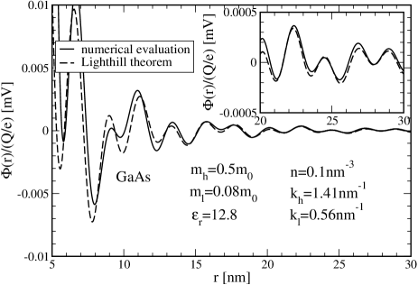
Figure 1: Friedel oscillations resulting from a numerical evaluation of the Fourier integral (9), and estimated via the Lighthill theorem (cf. Eq. (10)) for $p$-doped GaAs with a hole density of $n=10^{20}{\rm cm}^{-3}$. The inset shows the data at larger distances on a smaller scale.

The beating of Friedel oscillations illustrated in the figure is a peculiarity of the holes residing in the p-type valence band and should be observable via similar scanning tunneling microscopy techniques as used in metals Crommie93 and $n$-doped semiconductors Kanisawa01 . Moreover, as theoretical studies have revealed, such oscillations can have a profound impact on the magnetic properties of ferromagnetic semiconductors Schliemann02 ; Fiete05 . Moreover, Fig. 1 shows the amazing accuracy of the asymptotic expression (10) obtained from the Lighthill theorem.

Let us now turn to the regime of large frequencies and small wave vectors. Following Ref. Mahan00 we expand the denominators in Eq. (3) assuming $\hbar\omega>>\varepsilon_{h/l}(\vec{k})$ and $\hbar\omega>>(\hbar k_{h/l}/m_{h/l})\hbar k$. Within the two leading orders one finds

$$\varepsilon^{RPA}(\vec{k},\omega)=1-\frac{1}{\omega^{2}}\frac{e^{2}}{\varepsilon_{r}\varepsilon_{0}}\frac{1}{6\pi^{2}}\left(\frac{1}{m_{h}}+\frac{1}{m_{l}}\right)\left(k_{h}^{3}+k_{l}^{3}\right)$$

$$\qquad-\frac{1}{\omega^{4}}\frac{e^{2}\hbar^{2}}{\varepsilon_{r}\varepsilon_{0}\pi^{2}}\frac{1}{2}\left(\frac{1}{m_{h}^{3}}+\frac{1}{m_{l}^{3}}\right)\Biggl{[}\frac{1}{5}k^{2}\left(k_{h}^{5}+k_{l}^{5}\right)$$

$$\qquad\qquad+\frac{1}{12}k^{4}\left(k_{h}^{3}+k_{l}^{3}\right)\Biggr{]}$$

$$\qquad-\frac{1}{\omega^{4}}\frac{e^{2}\hbar^{2}}{\varepsilon_{r}\varepsilon_{0}\pi^{2}}\Biggl{[}-\frac{1}{56}\left(\frac{1}{m_{h}^{3}}-\frac{1}{m_{l}^{3}}\right)\left(k_{h}^{7}-k_{l}^{7}\right)$$

$$\qquad\qquad+\frac{3}{56}\left(\frac{1}{m_{h}}-\frac{1}{m_{l}}\right)^{2}\left(\frac{k_{h}^{7}}{m_{h}}+\frac{k_{l}^{7}}{m_{l}}\right)$$

$$\qquad\qquad+\frac{3}{28}\left(\frac{1}{m_{h}}-\frac{1}{m_{l}}\right)\left(\frac{k_{h}^{7}}{m_{h}^{2}}-\frac{k_{l}^{7}}{m_{l}^{2}}\right)$$

$$\qquad\qquad+\frac{21}{200}k^{2}\left(\frac{1}{m_{h}^{3}}-\frac{1}{m_{l}^{3}}\right)\left(k_{h}^{5}-k_{l}^{5}\right)$$

$$\qquad\qquad-\frac{3}{40}k^{2}\left(\frac{1}{m_{h}}-\frac{1}{m_{l}}\right)\left(\frac{k_{h}^{5}}{m_{h}^{2}}-\frac{k_{l}^{5}}{m_{l}^{2}}\right)\Biggr{]}$$ (12)

For $m_{h}=m_{l}$ the first three lines of the above expression reproduce again the standard textbook result Mahan00 while all other terms vanish in this limit. On the other hand, if $m_{h}\neq m_{l}$, one has contributions in order $1/\omega^{4}$ that are independent of the wave vector $\vec{k}$. Such terms are absent in the case of the standard electron gas where the contributions of order $1/\omega^{2n}$ are at least of order $k^{2n-2}$ in the wave vector Mahan00 . The technical reason why such contributions are present for the hole gas is that the expression $\varepsilon_{\lambda_{2}}(\vec{k}^{\prime}+\vec{k})-\varepsilon_{\lambda_{1}}(\vec{k}^{\prime})$ in Eq.(3) contains for $|\lambda_{1}|\neq|\lambda_{2}|$ an additive term which is independent of $k$ (and vanishes for $m_{h}=m_{l}$). These prima vista unexpected contributions to the high-frequency expansion of the dielectric function will also occur in even higher orders. However, even in the two leading orders given in Eq. (12), they strongly modify the plasmon dispersion determined by $\varepsilon^{RPA}(\vec{k},\omega(k))=0$ which can be expressed as

$$\omega^{2}(k)=\left(\omega_{p}^{(0)}\right)^{2}\Biggl{[}\frac{1}{2}+\frac{1}{2}\Bigl{[}1+4\Bigl{(}u\left(n^{1/3}a_{0}\right)$$

$$\qquad\qquad+\left(v+w\right)\frac{(ka_{0})^{2}}{n^{1/3}a_{0}}\Bigr{)}\Bigr{]}^{1/2}\Biggr{]}+{\cal O}\left(k^{4}\right)$$ (13)

$$\approx\left(\omega_{p}^{(0)}\right)^{2}\left(1+u\left(n^{1/3}a_{0}\right)+\left(v+w\right)\frac{(ka_{0})^{2}}{n^{1/3}a_{0}}\right)$$ (14)

where the zero-order plasma frequency is given bynote

$$\left(\omega_{p}^{(0)}\right)^{2}=\frac{e^{2}}{\varepsilon_{r}\varepsilon_{0}}\frac{n}{2}\left(\frac{1}{m_{h}}+\frac{1}{m_{l}}\right)\,,$$ (15)

and the dimensionless and density-independent coefficients $u$, $v$, $w$ are given by

$$u=\frac{Q\left(m_{h},m_{l}\right)}{\left(3\pi^{2}\right)^{1/3}\left(m_{h}^{3/2}+m_{l}^{3/2}\right)^{2/3}}$$

$$\quad\times\Biggl{[}-\frac{3}{14}\left(\frac{1}{m_{h}^{3}}-\frac{1}{m_{l}^{3}}\right)\left(m_{h}^{7/2}-m_{l}^{7/2}\right)$$

$$\qquad\qquad+\frac{9}{14}\left(\frac{1}{m_{h}}-\frac{1}{m_{l}}\right)^{2}\left(m_{h}^{5/2}+m_{l}^{5/2}\right)$$

$$\qquad\qquad+\frac{9}{7}\left(\frac{1}{m_{h}}-\frac{1}{m_{l}}\right)\left((m_{h}^{3/2}-m_{l}^{3/2}\right)\Biggr{]}\,,$$ (16)

$$v=Q\left(m_{h},m_{l}\right)\frac{2}{5\pi^{2}}\left(\frac{1}{m_{h}^{3}}+\frac{1}{m_{l}^{3}}\right)\left(m_{h}^{5/2}+m_{l}^{5/2}\right)\,,$$ (17)

$$w=Q\left(m_{h},m_{l}\right)\Biggl{[}\frac{21}{50\pi^{2}}\left(\frac{1}{m_{h}^{3}}-\frac{1}{m_{l}^{3}}\right)\left(m_{h}^{5/2}-m_{l}^{5/2}\right)$$

$$\qquad\qquad-\frac{3}{10\pi^{2}}\left(\frac{1}{m_{h}}-\frac{1}{m_{l}}\right)\left(m_{h}^{1/2}-m_{l}^{1/2}\right)\Biggr{]}$$ (18)

with the common prefactor

$$Q\left(m_{h},m_{l}\right)\frac{\frac{\varepsilon_{r}}{4\pi}m_{0}}{\left(\frac{1}{m_{h}}+\frac{1}{m_{l}}\right)^{2}}\frac{(3\pi^{2})^{5/3}}{\left(m_{h}^{3/2}+m_{l}^{3/2}\right)^{5/3}}\,.$$ (19)

Clearly, the coefficients $u$ and $w$ vanish for $m_{h}=m_{l}$ while from $v$ one recovers usual textbook result for an electron gas without spin-orbit coupling Mahan00 . By expanding the square root in Eq. (13) we have neglected higher contributions both in wave vector and in the density parameter $n^{1/3}a_{0}\propto(\varepsilon_{F}/\hbar\omega_{p}^{(0)})^{2}$ which is consistent with considering only the first two leading orders in Eq. (12). In fact, for usual $p$-doped bulk semiconductors $n^{1/3}a_{0}$ is small, and to consistently obtain contributions to the plasmon dispersion being of higher order in the density would require to extend the expansion (12) also to higher orders, which is computationally increasingly tedious and will lead to even lengthier expressions.

	$\frac{m_{h}}{m_{0}}$	$\frac{m_{l}}{m_{0}}$	$\varepsilon_{r}$	$\frac{m_{l}}{m_{h}}$	$u$	$v$	$w$
AlAs	0.47	0.18	10.0	0.38	17.7	21.5	-16.3
AlSb	0.36	0.13	12.0	0.36	49.7	37.1	-29.5
GaAs	0.5	0.08	12.8	0.16	195.4	99.4	-100.5
InAs	0.5	0.026	14.5	0.052	861.4	451.9	-473.1
InSb	0.2	0.015	18.0	0.075	1796.9	919.2	-958.8

Table 1: Material parameter and coefficients $u$, $v$, $w$ of the plasmon dispersion (14) for various III-V semiconductors.

Note that the dispersion coefficients $u$, $v$, $w$ depend entirely on material parameters. In table 1 we have listed their numerical values for several prominent III-V semiconductor systems. As seen there, the coefficient $u$ is remarkably large leading to a substantial enhancement of the long-wavelength plasma frequency $\omega^{2}(0)=(\omega_{p}^{(0)})^{2}(1+u(n^{1/3}a_{0})$, even at small densities, compared to the naive guess $\omega^{2}(0)\approx(\omega_{p}^{(0)})^{2}$. On the other hand, $v$ and $w$ differ in sign and are of quite similar magnitude resulting in a dramatic flattening of the plasma dispersion compared to the standard case $m_{h}=m_{l}$ where $w$ vanishes. Moreover, the sum $v+w$ can even become negative leading to a plasmon dispersion bending downwards around zero wave vector. In fact the sign of $v+w$ is entirely determined by the ratio $m_{l}/m_{h}$ where negative values occur for $m_{l}/m_{h}\lesssim 0.18$. Remarkably, GaAs lies very close this threshold showing already such a qualitative change in the plasmon dispersion. This trend is further enhanced in the cases of InAs and InSb.

In summary, we have studied the dielectric function of the homogeneous hole gas in $p$-doped zinc-blende III-V semiconductors. In the static limit we predict additional beatings of the Friedel oscillations which should be experimentally detectable via state-of-the-art scanning tunneling microscopy. At high frequencies and small wave vectors the plasmon dispersion gets dramatically altered compared to the textbook case of the usual electron gas.

I thank J. Repp for useful discussions and Deutsche Forschungsgemeinschaft for support via SFB 689.

References

• (1) G.Β F. Giuliani and G. Vignale, Quantum Theory of the Electron Liquid, Cambridge University Press 2005.
• (2) G. Mahan, Many-Particle Physics, 3rd edition, Kluwer, New York, 2000.
• (3) H. Bruus and K. Flensberg, Many-Body Quantum Theory in Condensed Matter Physics, Cambridge University Press 2004.
• (4) T. Jungwirth, J. Sinova, J. Masek, J. Kucera, and A. H. MacDonald, Rev. Mod. Phys. 78, 809 (2006).
• (5) J. Fabian, A. Matos-Abiague, C. Ertler, P. Stano, and I. Zutic, Acta. Phys. Slov. 57, 565 (2007).
• (6) J.Β M. Luttinger, Phys. Rev. 102, 1030 (1956).
• (7) J. Schliemann, Phys. Rev. B 74, 045214 (2006).
• (8) M. Pletyukhov and V. Gritsev, Phys. Rev. B 74, 045307 (2006).
• (9) S.Β M. Badalyan, A. Matos-Abiague, G. Vignale, and J. Fabian, Phys. Rev. B 79, 205305 (2009); ibid. 81, 205314 (2010).
• (10) S.-J. Cheng and R.Β R. Gerhardts, Phys. Rev. B 63, 035314 (2001); V. Lopez-Richard, G.Β E. Marques, and C. Trallero-Giner, J. Appl. Phys. 89, 6400 (2001); T. Kernreiter, M. Governale, and U. Zulicke, New J. Phys. 12, 093002 (2010).
• (11) B. Wunsch, T. Stauber, F. Sols, and F. Guinea, New J. Phys. 8, 318 (2006); E.Β H. Hwang and S. Das Sarma, Phys. Rev. B 75, 205418 (2007).
• (12) T. Stauber, J. Schliemann, and N.Β M.Β R. Peres, Phys. Rev. B 81, 085409 (2010).
• (13) G.Β E. Simion and G.Β F. Giuliani, Phys. Rev. B 72, 045127 (2005)
• (14) M.Β J. Lighthill, An Introduction to Fourier Analysis and Generalised Functions, Cambridge University Press 1958.
• (15) M.Β F. Crommie, C.Β P. Lutz, and D.Β M. Eigler, Nature 363, 524 (1993).
• (16) K. Kanisawa, M.Β J. Butcher, H. Yamaguchi, and Y. Hirayama, Phys. Rev. Lett. 86, 3384 (2001); K. Suzuki, K. Kanisawa, C. Janer, S. Perraud, K. Takashina, T. Fujisawa, and Y. Hirayama, Phys. Rev. Lett. 98, 136802 (2007).
• (17) J. Schliemann and A. H. MacDonald, Phys. Rev. Lett. 88, 137201 (2002); J. Schliemann, Phys. Rev. B 67, 045202 (2003).
• (18) G.Β A. Fiete, G. Zarand, B. Janko, P. Redlinski, and C. Pascu Moca, Phys. Rev. B 71, 115202 (2005).
• (19) The lowest-order resultΒ (15) for the plasma frequency differs in detail from the one given in Ref.Β Schliemann06 due to a somewhat oversimplified approach there.