Non-Markovian theory of vibrational energy relaxation and its applications to biomolecular systems

I Introduction

Energy transfer (relaxation) phenomena are ubiquitous in nature. At a macroscopic level, the phenomenological theory of heat (Fourier law) successfully describes heat transfer and energy flow. However, its microscopic origin is still under debate. This is because the phenomena can contain many-body, multi-scale, nonequilibrium, and even quantum mechanical aspects, which present significant challenges to theories addressing energy transfer phenomena in physics, chemistry and biology Johnbook . For example, heat generation and transfer in nano-devices is a critical problem in the design of nanotechnology. In molecular physics, it is well known that vibrational energy relaxation (VER) is an essential aspect of any quantitative description of chemical reactions Nitzan . In the celebrated RRKM theory of an absolute reaction rate for isolated molecules, it is assumed that the intramolecular vibrational energy relaxation (IVR) is much faster than the reaction itself. Under certain statistical assumptions, the reaction rate can be derived Steinfeldbook . For chemical reactions in solutions, the transition state theory and its extension such as Kramer’s theory and the Grote-Hynes theory have been developed Billingbook ; BBS88 and applied to a variety of chemical systems including biomolecular systems PTMHR08 . However, one cannot always assume that separation of timescales. It has been shown that a conformational transition (or reaction) rate can be modulated by the IVR rate LW97 . As this brief survey demonstrates, a detailed understanding of IVR or VER is essential to study the chemical reaction and conformation change of molecules.

A relatively well understood class of VER is a single vibrational mode embedded in (vibrational) bath modes. If the coupling between the system and bath modes is weak (or assumed to be weak), a Fermi’s-golden-rule style formula derived using 2nd order perturbation theory Oxtoby79 ; RMH04 ; LS02 may be used to estimate the VER rate. However, the application of such theories to real molecular systems poses several (technical) challenges, including how to choose force fields, how to separate quantum and classical degrees of freedom, or how to treat the separation of timescales between system and bath modes. Multiple solutions have been proposed to meet those challenges leading to a variety of theoretical approaches to the treatment of VER Okazaki ; Leitner ; Leitner09 ; Pouthier08 ; Knoester07 ; Knoester08 . These works using Fermi’s golden rule are based on quantum mechanics and suitable for the description of high frequency modes (more than thermal energy $\simeq$ 200 cm^-1), on which nonlinear spectroscopy has recently focused Hochstrasser ; MK97 ; Dlott03 ; Hamm08 .

In this chapter, we summarize our recent work on VER of high frequency modes in biomolecular systems. In our previous work, we have concentrated on the VER rate and mechanisms for proteins Fujisaki05 . Here we shall focus on the time course of the VER dynamics. We extend our previous Markovian theory of VER to a non-Markovian theory applicable to a broader range of chemical systems FZS06 ; FS07 . Recent time-resolved spectroscopy can detect the time course of VER dynamics (with femto-second resolution), which may not be accurately described by a single time scale. We derive new formulas for VER dynamics, and apply them to several interesting cases, where comparison to experimental data is available.

This chapter is organized as follows: In Sec. II, we briefly summarize the normal mode concepts in protein dynamics simulations, on which we build our non-Markovian VER theory. In Sec. III, we derive VER formulas under several assumptions, and discuss the limitations of our formulas. In Sec. IV, we apply the VER formulas to several situations: the amide I modes in solvated $N$-methylacetamide and cytochrome c, and two in-plane modes ($\nu_{4}$ and $\nu_{7}$ modes) in a porphyrin ligated to imidazol. We employ a number of approximations in describing the potential energy surface on which the dynamics takes place, including the empirical CHARMM CHARMM force field and density functional calculations Gaussian for the small parts of the system ($N$-methylacetamide and porphyrin). We compare our theoretical results with experiment when available, and find good agreement. We can deduce the VER mechanism based on our theory for each case. In Sec. V, we summarize and discuss the further aspects of VER in biomolecules and in nanotechnology (molecular devices).

II Normal mode concepts applied to protein dynamics

Normal mode provides a powerful tool in exploring molecular vibrational dynamics Wilsonbook and may be applied to biomolecules as well CuiBaharbook . The first normal mode calculations for a protein were performed for BPTI protein GNN83 . Most biomolecular simulation softwares support the calculation of normal modes CHARMM ; Gromacs ; Amber . However, the calculation of a mass-weighted hessian $K_{ij}$, which requires the second derivatives of the potential energy surface, with elements defined as

$$K_{ij}=\frac{1}{\sqrt{m_{i}m_{j}}}\frac{\partial^{2}V}{\partial x_{i}\partial x_{j}}$$ (1)

can be computational demanding. Here $m_{i}$ is the mass, $x_{i}$ is the coordinate, and $V$ is the potential energy of the system. Efficient methods have been devised including torsional angle normal mode Wako , block normal mode TGMS00 , and the iterative mixed-basis diagonalization (DIMB) methods MP93 etc. An alternative direction for the efficient calculations of a hessian is to use coarse-grained models such as elastic Tirion or Gaussian network HBE97 models. From normal mode analysis (or instantaneous normal mode analysis Keyes ), the frequencies, density of states, and normal mode vectors can be calculated. In particular, the latter quantity is important because it is known that the lowest eigenvectors may describe the functionally important motions such as large-scale conformational change, a subject that is the focus of another chapter in this volume FMK09 .

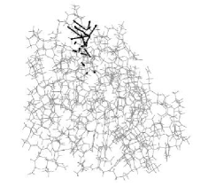
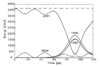
Figure 1: Left: The excited eigenvector depicted by arrows in myoglobin. Right: Classical simulation of mode specific energy transfer in myoglobin at zero temperature. [Reprinted with permission from K. Moritsugu, O. Miyashita and A. Kidera, Phys. Rev. Lett. 85, 3970 (2000). Copyright ©2009 by the American Physical Society.]

There is no doubt as to the usefulness of normal mode concepts. However, for molecular systems, it is always an approximate model as higher-order nonlinear coupling and intrinsic anharmonicity become essential. To describe energy transfer (or relaxation) phenomena in a protein, Moritsugu, Miyashita, and Kidera (MMK) introduced a reduced model using normal modes with 3rd and 4th order anharmonicity MMK00 , $C_{klm}^{(3)}$ and $C_{klmn}^{(4)}$, respectively,

$$V(\{q_{k}\})=\sum_{k}\frac{\omega_{k}^{2}}{2}q_{k}^{2}+\frac{1}{3!}\sum_{klm}C_{klm}^{(3)}q_{k}q_{l}q_{m}+\frac{1}{4!}\sum_{klmn}C_{klmn}^{(4)}q_{k}q_{l}q_{m}q_{n}$$ (2)

with

$$C_{klm}^{(3)} \equiv \frac{\partial^{3}V}{\partial q_{k}\partial q_{l}\partial q_{m}},$$ (3)

$$C_{klmn}^{(4)} \equiv \frac{\partial^{4}V}{\partial q_{k}\partial q_{l}\partial q_{m}\partial q_{n}}$$ (4)

where $q_{k}$ denotes the normal mode calculated by the hessian $K_{ij}$ and $\omega_{k}$ is the normal mode frequency. Classical (and harmonic) Fermi resonance Kubobook is a key ingredient in the MMK theory of energy transfer derived from observations of all-atom simulations of myoglobin at zero temperature (see Fig. 1).

At finite temperature, non-resonant effects become important and clear interpretation of the numerical results becomes difficult within the classical approximation. Nagaoka and coworkers Nagaoka identified essential vibrational modes in vacuum simulations of myoglobin and connected these modes to the mechanism of “heme cooling” explored experimentally by Mizutani and Kitagawa MK97 . Contemporaneously, nonequilibrium MD simulations of solvated myoglobin carried out by Sagnella and Straub provided the first detailed and accurate simulation of heme cooling dynamics Straub . That work provided support for the conjecture that the motion similar to those modes identified by Nagaoka play an important role in energy flow pathways.

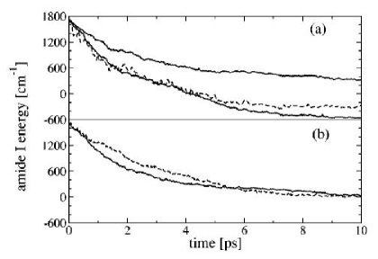
Figure 2: Nonequilibrium MD simulation of energy flow from the excited amide I mode in $N$-methylacetamide in heavy water. See also Fig. 3. [Reprinted with permission from P.H. Nguyen and G. Stock, J. Chem. Phys. 119, 11350 (2003). Copyright ©2009 by the American Institute of Physics.]

Nguyen and Stock explored the vibrational dynamics of the small molecule, $N$-methylacetamide (NMA), often used as a model of the peptide backbone Stock . Using nonequilibrium MD simulations of NMA in heavy water, VER was observed to occur on a pico-second time scale for the amide I vibrational mode (see Fig. 2). They used the instantaneous normal mode concept Keyes to interpret their result and noted the essential role of anharmonic coupling. Leitner also used the normal mode concept to describe energy diffusion in a protein, and found an interesting link between the anomalous heat diffusion and the geometrical properties of a protein YL03 .

In terms of vibrational spectroscopy, Gerber et al. calculated the anharmonic frequencies in BPTI, within the VSCF level of theory Gerber , using the reduced model (2). Yagi, Hirata, and Hirao refined this type of anharmoic frequency calculation for large molecular systems with more efficient methods Yagi , appropriate for applications to biomolecules such as DNA base pair Yagi2 . Based on the reduced model (2) with higher-order nonlinear coupling, Leitner also studied quantum mechanical aspects of VER in proteins, by employing the Maradudin-Fein theory based on Fermi’s “Golden Rule” Leitner . Using the same model, Fujisaki, Zhang, and Straub focused on more detailed aspects of VER in biomolecular systems, and calculated the VER rate, mechanisms or pathways, using their non-Markovian perturbative formulas (described below).

As this brief survey demonstrates, the normal mode concept is a powerful tool that provides significant insight into mode specific vibrational dynamics and energy transfer in proteins.

III Derivation of non-Markovian VER formulas

We have derived a VER formula for the simplest situation, a one-dimensional relaxing oscillator coupled to a “static” bath FZS06 . Here we extend this treatment to two more general directions: (a) multi-dimensional relaxing modes coupled to a “static” bath and (b) a one-dimensional relaxing mode coupled to a “fluctuating” bath FS08 .

III.1 Multi-dimensional relaxing mode coupled to a static bath

We take the following time-independent Hamiltonian

$${\cal H} = {\cal H}^{0}_{S}+{\cal H}_{B}+{\cal V}^{0}$$ (5)

$$= {\cal H}^{0}_{S}+\langle{\cal V}\rangle_{B}+{\cal H}_{B}+{\cal V}^{0}-\langle{\cal V}\rangle_{B}$$ (6)

$$= {\cal H}_{S}+{\cal H}_{B}+{\cal V}$$ (7)

where

$${\cal H}_{S} \equiv {\cal H}^{0}_{S}+\langle{\cal V}\rangle_{B},$$ (8)

$${\cal V} \equiv {\cal V}^{0}-\langle{\cal V}\rangle_{B}.$$ (9)

In previous work FZS06 , we have considered only a single one-dimensional oscillator as the system. Here we extend that treatment to the case of an $N_{S}$-dimensional oscillator system. That is,

$${\cal H}_{S} = \sum_{i=1}^{N_{S}}\left(\frac{p_{i}^{2}}{2}+\frac{\omega_{i}^{2}}{2}q_{i}^{2}\right)+V(\{q_{i}\}),$$ (10)

$${\cal H}_{B} = \sum_{\alpha=1}^{N_{B}}\left(\frac{p_{\alpha}^{2}}{2}+\frac{\omega_{\alpha}^{2}}{2}q_{\alpha}^{2}\right),$$ (11)

$${\cal V} = -\sum_{i=1}^{N_{S}}q_{i}\delta{\cal F}_{i}(\{q_{\alpha}\})$$ (12)

where $V(\{q_{i}\})$ is the interaction potential function between $N_{S}$ system modes which can be described by, for example, the reduced model, Eq. (2). The simplest case $V(\{q_{i}\})=0$ is trivial as each system mode may be treated seperately within the perturbation approximation for ${\cal V}$.

We assume that $|k\rangle$ is a certain state in the Hilbert space spanned by ${\cal H}_{S}$. Then the reduced density matrix is

$$(\rho_{S})_{mn}(t) = \langle m|e^{-i{\cal H}_{S}t/\hbar}{\rm Tr}_{B}\{\tilde{\rho}(t)\}e^{i{\cal H}_{S}t/\hbar}|n\rangle$$ (13)

where tilde denotes the interaction picture. Substituting the time-dependent perturbation expansion

$$\tilde{\rho}(t) = \rho(0)+\frac{1}{i\hbar}\int_{0}^{t}dt^{\prime}[\tilde{\cal V}(t^{\prime}),\rho(0)]$$ (14)

$$+\frac{1}{(i\hbar)^{2}}\int_{0}^{t}dt^{\prime}\int_{0}^{t^{\prime}}dt^{\prime\prime}[\tilde{\cal V}(t^{\prime}),[\tilde{\cal V}(t^{\prime\prime}),\rho(0)]]+\cdots$$

into the above, we find

$$(\rho_{S})_{mn}(t) \simeq (\rho_{S})^{(0)}_{mn}(t)+(\rho_{S})^{(1)}_{mn}(t)+(\rho_{S})^{(2)}_{mn}(t)+\cdots,$$ (15)

where

$$(\rho_{S})^{(0)}_{mn}(t) = \langle m|e^{-i{\cal H}_{S}t/\hbar}{\rho}_{S}(0)e^{i{\cal H}_{S}t/\hbar}|n\rangle,$$ (16)

$$= \langle m(-t)|{\rho}_{S}(0)|n(-t)\rangle=\langle m|{\rho}_{S}(t)|n\rangle$$

$$(\rho_{S})^{(2)}_{mn}(t) = \frac{1}{(i\hbar)^{2}}\int^{t}_{0}dt^{\prime}\int^{t^{\prime}}_{0}dt^{\prime\prime}\langle m|e^{-i{\cal H}_{S}t/\hbar}{\rm Tr}_{B}\{[\tilde{\cal V}(t^{\prime}),[\tilde{\cal V}(t^{\prime\prime}),\rho(0)]]\}e^{i{\cal H}_{S}t/\hbar}|n\rangle$$ (17)

$$= \frac{1}{(i\hbar)^{2}}\int_{0}^{t}dt^{\prime}\int_{0}^{t^{\prime}}dt^{\prime\prime}\sum_{i,j}\langle m(-t)|[q_{i}(t^{\prime})q_{j}(t^{\prime\prime})\rho_{S}(0)$$

$$-q_{j}(t^{\prime\prime})\rho_{S}(0)q_{i}(t^{\prime})]|n(-t)\rangle\langle\delta{\cal F}_{i}(t^{\prime})\delta{\cal F}_{j}(t^{\prime\prime})\rangle_{B}$$

$$+ \frac{1}{(i\hbar)^{2}}\int_{0}^{t}dt^{\prime}\int_{0}^{t^{\prime}}dt^{\prime\prime}\sum_{i,j}\langle m(-t)|[\rho_{S}(0)q_{j}(t^{\prime\prime})q_{i}(t^{\prime})$$

$$-q_{i}(t^{\prime})\rho_{S}(0)q_{j}(t^{\prime\prime})]|n(-t)\rangle\langle\delta{\cal F}_{j}(t^{\prime\prime})\delta{\cal F}_{i}(t^{\prime})\rangle_{B}.$$

Here we have defined $|m(t)\rangle=e^{-i{\cal H}_{S}t/\hbar}|m\rangle$ and taken $(\rho_{S})^{(1)}_{mn}(t)=0$. Recognizing that we must evaluate expressions of the form

$$R_{mn;ij}(t;t^{\prime},t^{\prime\prime}) = \langle m(-t)|[q_{i}(t^{\prime})q_{j}(t^{\prime\prime})\rho_{S}(0)|n(-t)\rangle,$$ (18)

$$-\langle m(-t)|q_{j}(t^{\prime\prime})\rho_{S}(0)q_{i}(t^{\prime})]|n(-t)\rangle$$

$$C_{ij}(t^{\prime},t^{\prime\prime}) = \langle\delta{\cal F}_{i}(t^{\prime})\delta{\cal F}_{j}(t^{\prime\prime})\rangle_{B}$$ (19)

and their complex conjugates, $R^{*}_{nm;ij}(t;t^{\prime},t^{\prime\prime}),C^{*}_{ij}(t^{\prime},t^{\prime\prime})$, the 2nd order contribution can be written

$$(\rho_{S})^{(2)}_{mn}(t) = \frac{1}{(i\hbar)^{2}}\int^{t}_{0}dt^{\prime}\int^{t^{\prime}}_{0}dt^{\prime\prime}\sum_{i,j}[R_{mn;ij}(t;t^{\prime},t^{\prime\prime})C_{ij}(t^{\prime},t^{\prime\prime})$$ (20)

$$+R^{*}_{nm;ij}(t;t^{\prime},t^{\prime\prime})C^{*}_{ij}(t^{\prime},t^{\prime\prime})].$$

We can seperately treat the two terms. Assuming that we can solve ${\cal H}_{S}|a\rangle=E_{a}|a\rangle$, we find

$$R_{mn;ij}(t;t^{\prime},t^{\prime\prime}) = \sum_{abcd}\langle m|a\rangle(q_{i})_{ab}(q_{j})_{bc}(\rho_{S})_{cd}\langle d|n\rangle$$ (21)

$$\times e^{-i(E_{a}-E_{d})t-i(E_{b}-E_{a})t^{\prime}-i(E_{c}-E_{b})t^{\prime\prime}}$$

$$- \sum_{abcd}\langle m|a\rangle(q_{j})_{ab}(\rho_{S})_{bc}(q_{i})_{cd}\langle d|n\rangle$$

$$\times e^{-i(E_{a}-E_{d})t-i(E_{d}-E_{c})t^{\prime}-i(E_{b}-E_{a})t^{\prime\prime}}$$

For the bath-averaged term, we assume the following force due to third-order nonlinear coupling of system mode $i$ to the normal modes, $\alpha$ and $\beta$, of the bath Fujisaki05

$$\delta{\cal F}_{i}(\{q_{\alpha}\})=\sum_{\alpha,\beta}C_{i\alpha\beta}(q_{\alpha}q_{\beta}-\langle q_{\alpha}q_{\beta}\rangle)$$ (22)

and we have Fujisaki05

$$C_{ij}(t^{\prime},t^{\prime\prime})=R^{--}_{ij}(t^{\prime},t^{\prime\prime})+R^{++}_{ij}(t^{\prime},t^{\prime\prime})+R^{+-}_{ij}(t^{\prime},t^{\prime\prime})$$ (23)

with

$$R^{--}_{ij}(t^{\prime},t^{\prime\prime}) = \frac{\hbar^{2}}{2}\sum_{\alpha,{\beta}}D_{\alpha{\beta};ij}(1+n_{\alpha})(1+n_{{\beta}})e^{-i(\omega_{\alpha}+\omega_{{\beta}})(t^{\prime}-t^{\prime\prime})},$$ (24)

$$R^{++}_{ij}(t^{\prime},t^{\prime\prime}) = \frac{\hbar^{2}}{2}\sum_{{\alpha},{\beta}}D_{{\alpha}{\beta};ij}n_{\alpha}n_{{\beta}}e^{i(\omega_{\alpha}+\omega_{{\beta}})(t^{\prime}-t^{\prime\prime})},$$ (25)

$$R^{+-}_{ij}(t^{\prime},t^{\prime\prime}) = \hbar^{2}\sum_{\alpha,{\beta}}D_{{\alpha}{\beta};ij}(1+n_{\alpha})n_{\beta}e^{-i(\omega_{\alpha}-\omega_{{\beta}})(t^{\prime}-t^{\prime\prime})}$$ (26)

where

$$D_{\alpha\beta;ij}=\frac{C_{i\alpha\beta}C_{j\alpha\beta}}{\omega_{\alpha}\omega_{\beta}}$$ (27)

and $n_{\alpha}$ is the thermal population of the bath mode $\alpha$.

This formula reduces to our previous result for a one-dimensional system oscillator FZS06 when $N_{S}=1$ and all indices $(i,j)$ are suppressed. Importantly, this formula can be applied to situations where it is difficult to define a “good” normal mode to serve as a one-dimensional relaxing mode, as in the case of the CH stretching modes of a methyl group Fujisaki05 . However, expanding to an $N_{S}$ dimensional system adds the burden of solving the multidimensional Schrödinger equation ${\cal H}_{S}|a\rangle=E_{a}|a\rangle$. To address this challenge we may employ vibrational self-consistent field (VSCF) theory and its extensions developed by Bowman and coworkers Bowman implemented in MULTIMODE program of Carter and Bowman MULTIMODE or in the SINDO program sindo of Yagi and coworkers. As in the case of our previous theory of a one-dimensional system mode, we must calculate $N_{S}$-tiple 3rd order coupling constants $C_{i\alpha\beta}(i=1,2,...N_{S})$ for all bath modes $\alpha$ and $\beta$.

III.2 One-dimensional relaxing mode coupled to a fluctuating bath

We start from the following time-dependent Hamiltonian

$${\cal H}(t) = {\cal H}^{0}_{S}(t)+{\cal H}_{B}(t)+{\cal V}^{0}(t)$$ (28)

$$= {\cal H}^{0}_{S}(t)+\langle{\cal V}(t)\rangle_{B}+{\cal H}_{B}(t)+{\cal V}^{0}(t)-\langle{\cal V}(t)\rangle_{B}$$ (29)

$$= {\cal H}_{S}(t)+{\cal H}_{B}(t)+{\cal V}(t)$$ (30)

where

$${\cal H}_{S}(t) \equiv {\cal H}^{0}_{S}(t)+\langle{\cal V}(t)\rangle_{B},$$ (31)

$${\cal V}(t) \equiv {\cal V}^{0}(t)-\langle{\cal V}(t)\rangle_{B}$$ (32)

with the goal of solving the time-dependent Schrödinger equation

$$i\hbar\frac{\partial|\Psi(t)\rangle}{\partial t}=[{\cal H}_{S}(t)+{\cal H}_{B}(t)+{\cal V}(t)]|\Psi(t)\rangle=[{\cal H}_{0}(t)+{\cal V}(t)]|\Psi(t)\rangle.$$ (33)

By introducing a unitary operator $U_{0}(t)=U_{S}(t)U_{B}(t)$

$$i\hbar\frac{d}{dt}U_{0}(t) = {\cal H}_{0}(t)U_{0}(t),$$ (34)

$$i\hbar\frac{d}{dt}U_{S}(t) = {\cal H}_{S}(t)U_{S}(t),$$ (35)

$$i\hbar\frac{d}{dt}U_{B}(t) = {\cal H}_{B}(t)U_{B}(t),$$ (36)

we can derive an “interaction picture” von Neumann equation

$$i\hbar\frac{d}{dt}\tilde{\rho}(t)=[\tilde{\cal V}(t),\tilde{\rho}(t)]$$ (37)

where

$$\tilde{\cal V}(t) = U_{0}^{\dagger}(t){\cal V}(t)U_{0}(t),$$ (38)

$$\tilde{\rho}(t) = U_{0}^{\dagger}(t)\rho(t)U_{0}(t).$$ (39)

We assume the simple form of a harmonic system and bath, but allow fluctuations in the system and bath modes modeled by time-dependent frequencies

$${\cal H}_{S}(t) = \hbar\omega_{S}(t)(a_{S}^{\dagger}a_{S}+1/2),$$ (40)

$${\cal H}_{B}(t) = \sum_{\alpha}\hbar\omega_{\alpha}(t)(a_{\alpha}^{\dagger}a_{\alpha}+1/2).$$ (41)

The unitary operators generated by these Hamiltonians are

$$U_{S}(t) = e^{-i\int_{0}^{t}d\tau\omega_{S}(\tau)(a_{S}^{\dagger}a_{S}+1/2)},$$ (42)

$$U_{B}(t) = e^{-i\int_{0}^{t}d\tau\sum_{\alpha}\omega_{\alpha}(\tau).(a_{\alpha}^{\dagger}a_{\alpha}+1/2)}$$ (43)

and the time evolution of the annihilation operators is given by

$$U_{S}^{\dagger}(t)a_{S}U_{S}(t) = a_{S}e^{-i\int_{0}^{t}d\tau\omega_{S}(\tau)},$$ (44)

$$U_{B}^{\dagger}(t)a_{\alpha}U_{B}(t) = a_{\alpha}e^{-i\int_{0}^{t}d\tau\omega_{\alpha}(\tau)}.$$ (45)

To simplify the evaluation of the force autocorrelation function, we assume that the temperature is low or the system mode frequency is high as a justification for the approximation. Substituting the above result into the force autocorrelation function calculated by the force operator, Eq. (22), we find

$$\langle\delta{\cal F}(t^{\prime})\delta{\cal F}(t^{\prime\prime})\rangle \simeq \frac{\hbar^{2}}{2}\sum_{\alpha,{\beta}}\frac{C_{S\alpha\beta}(t^{\prime})C_{S\alpha\beta}(t^{\prime\prime})}{\sqrt{\omega_{\alpha}(t^{\prime})\omega_{\beta}(t^{\prime})\omega_{\alpha}(t^{\prime\prime})\omega_{\beta}(t^{\prime\prime})}}$$ (46)

$$\times e^{-i[\Theta_{\alpha\beta}(t^{\prime})-\Theta_{\alpha\beta}(t^{\prime\prime})]}$$

where

$$\Theta_{S}(t) = \int_{0}^{t}d\tau\omega_{S}(\tau),$$ (47)

$$\Theta_{\alpha\beta}(t) = \int_{0}^{t}d\tau[\omega_{\alpha}(\tau)+\omega_{\beta}(\tau)].$$ (48)

Substituting this approximation into the perturbation expansion Eqs. (15), (16), and (17), we obtain our final result

$$(\rho_{S})_{00}(t) \simeq \frac{\hbar}{2}\sum_{\alpha,\beta}\int_{0}^{t}dt^{\prime}\int_{0}^{t^{\prime}}dt^{\prime\prime}\frac{C_{S\alpha\beta}(t^{\prime})C_{S\alpha\beta}(t^{\prime\prime})}{\sqrt{\omega_{S}(t^{\prime})\omega_{\alpha}(t^{\prime})\omega_{\beta}(t^{\prime})\omega_{S}(t^{\prime\prime})\omega_{\alpha}(t^{\prime\prime})\omega_{\beta}(t^{\prime\prime})}}$$ (49)

$$\times\cos\left\{\Theta_{S}(t^{\prime})-\Theta_{\alpha\beta}(t^{\prime})-\Theta_{S}(t^{\prime\prime})+\Theta_{\alpha\beta}(t^{\prime\prime})\right\}$$

which provides a dynamic correction to the previous formula FZS06 . The time-dependent parameters $\omega_{S}(t),\omega_{\alpha}(t),C_{S\alpha\beta}(t)$ may be computed from a running trajectory using instantaneous normal mode analysis Keyes . This result was first derived by Fujisaki and Stock FS08 , and applied to the VER dynamics of $N$-methylacetamide as described below. This correction eliminates the assumption that the bath frequencies are static on the VER timescale.

For the case of a static bath, the frequency and coupling parameters are time-independent and this formula reduces to the previous one-dimensional formula (when the off-resonant terms are neglected) FZS06 :

$$(\rho_{S})_{00}(t) \simeq \frac{\hbar}{2\omega_{S}}\sum_{\alpha,\beta}\frac{C_{S\alpha\beta}^{2}}{\omega_{\alpha}\omega_{\beta}}\frac{1-\cos[(\omega_{S}-\omega_{\alpha}-\omega_{\beta})t]}{(\omega_{S}-\omega_{\alpha}-\omega_{\beta})^{2}}.$$ (50)

Note that Bakker derived a similar fluctuating Landau-Teller formula in a different manner Bakker04 . It was successfully applied to molecular systems by Sibert and coworkers Sibert . However, the above formula differs from Bakker’s as (a) we use the instantaneous normal mode analysis to parameterize our expression, and (b) we do not take the Markov limit. Our formula can describe the time course of the density matrix as well as the VER rate.

One further point is that we use the cumulant-type approximation to calculate the dynamics. When we calculate an excited state probability, we use

$$(\rho_{S})_{11}(t)=1-(\rho_{S})_{00}(t)\simeq\exp\{-(\rho_{S})_{00}(t)\}.$$ (51)

Of course, this is valid for the initial process ($(\rho_{S})_{00}(t)\ll 1$), but, at longer time scales, we take $(\rho_{S})_{11}(t)\simeq\exp\{-(\rho_{S})_{00}(t)\}$ because the naive formula $(\rho_{S})_{11}(t)=1-(\rho_{S})_{00}(t)$ can be negative, which is unphysical FS08 .

III.3 Limitations of the VER formulas and comments

There are several limitations to the VER formulas derived above. The most obvious is that they are 2nd order perturbative formulas and rely on a short-time approximation. As far as we know, however, there exists no non-perturbative quantum mechanical treatment of VER applicable to large molecular systems. It is prohibitive to treat the full molecular dynamics quantum mechanically GW04 for large molecules. Moreover, while there exist several mixed quantum-classical methods Okazaki that may be applied to the study of VER, but there is no guarantee that such approximate methods work better than the perturbative treatment BB94 .

Another important limitation is the adaptation of a normal mode basis set, a natural choice for molecular vibrations. Because of the normal mode analysis, the computation can be burdensome. When we employ instantaneous normal mode analysis Keyes , there is a concern about the imaginary frequency modes. For the study of high frequency modes, this may not be significant. However, for the study of low frequency modes, the divergence of quantum (or classical) dynamics due to the presence of such imaginary frequency modes is a significant concern. For the study of low frequency modes, it is more satisfactory to use other methods that do not rely on normal mode analysis such as semiclassical methods Geva or path integral methods pathintegral .

We often use “empirical” force fields to describe quantum dynamics. However, it is well known that the force fields underestimate anharmonicity of molecular vibrations GCG02 . It is often desirable to use ab initio potential energy surfaces. However, that more rigorous approach can be demanding. Lower levels of theory can fail to match the accuracy of some empirical potentials. As a compromise, approximate potentials of intermediate accuracy, such as QM/MM potentials SF09 , may be appropriate. We discuss this question further in Sec. IV.1 and in Sec. IV.3.

IV Applications of the VER formulas to vibrational modes in biomolecules

We study the quantum dynamics of high frequency modes in biomolecular systems using a variety of VER formulas described in Sec. III. The application of a variety of theoretical approaches to essential VER processes will allow for a relative comparison of theories as well as the absolute assessment of theoretical predictions compared with experimental observations. In doing so, we address a number of fundamental questions. What are the limitations of the static bath approximation for fast VER in biomolecular systems? Can the relaxation dynamics of a relaxing amide I vibration in a protein be accurately modeled as a one-dimensional system mode coupled to a harmonic bath? Can the “fluctuating bath” model accurately capture the system dynamics when the static picture of normal modes is not “good” on the timescale of the VER process? In Sec. IV.1 and IV.2, our main focus is the VER of excited amide I modes in peptides or proteins. In Sec. IV.3, we study some vibrational modes in porphyrin ligated to imizadol, which is a mimic of a heme molecule in heme-proteins including myoglobin and hemoglobin.

IV.1 $N$-methylacetamide

$N$-methylacetamide (NMA) is a well-studied small molecule (CH₃-CO-NH-CH₃) that serves as a convenient model of a peptide bond structure (-CO-NH-) in theory and experiment. As in other amino acids, there is an amide I mode, localized on the CO bond stretch, which is a useful “reporter” of peptide structure and dynamics when probed by infrared spectrocopy. Many theoretical and experimental studies on amide I and other vibrational modes (amide II, III) have characterized how the mode frequencies depend on the local secondary structure of peptides or proteins Krimm ; TT92 . For the accurate description of frequencies and polarizability of these modes, see Refs. Knoester07 ; Knoester08 ; TT98 ; Skinnergroup ; HHC05 ; Mukamelgroup ; Stock06 . The main focus of these works is the frequency sensitivity of amide modes on the molecular configuration and environment. In this case, the amide mode frequencies are treated in a quantum mechanical way, but the configuration is treated classically. With a focus on interpreting mode frequency shifts due to configuration and environment, mode-coupling between amide modes and other modes is often neglected. As we are mainly interested in VER or IVR dynamics of these modes, an accurate treatment of the mode coupling is essential.

Recent theoretical development of IVR dynamics in small molecules is summarized in GW04 . Leitner and Wolynes LW97 utilized the concept of local random matrix to clarify the quantum aspects of such dynamics. The usefulness and applications of their approach are summarized in Leitner as well as in this volume Leitner09 . However, these studies are focused on isolated molecules, whereas our main interest is in exploring quantum dynamics in a condensed phase. We take a step-by-step hierarchical approach. Starting from the isolated NMA molecule, we add several water molecules to form NMA-water clusters, and finally treat the condensed phase NMA-water system (see Fig 3). With increasing complexity of our dynamical model, the accuracy of our theory, including the quality of the potential energy surface and the accuracy of the quantum dynamics must diminish. As such, a pricipal focus of our account is a careful examination and validation of our procedures through comparison with accurate methods or experiment.

Figure 3: Representation of three models employed for the study of VER dynamics in $N$-methylacetamide (NMA). (a) NMA, (b) NMA with three solvating water, (c) NMA with first solvation shell derived from simulations in bulk water. [Reprinted with permission for (a) and (b) from Y. Zhang, H. Fujisaki, and J.E. Straub, J. Phys. Chem. A 113, 3051 (2009). Copyright ©2009 by the American Chemical Society.] [Reprinted with permission for (c) from H. Fujisaki and G. Stock, J. Chem. Phys. 129,134110 (2008). Copyright ©2009 by the American Institute of Physics.]

IV.1.1 $N$-methylacetamide in vacuum

In our studies of isolated NMA FYHS07 ; FYSS09 , we have employed both accurate potential energy surface and accurate quantum dynamics methods to explore the timescale and mechanism of VER. From the anharmonic frequency calculations and comparison to experiment ATT84 , we concluded that B3LYP/6-31G(d) is a method of choice for computation of the electronic ground state potential surface, considering both accuracy and feasibility. For other treatments at differing levels of theory of quantum chemical calculation on NMA, see Refs. GCG02 ; BS06 ; KB07 . After the construction of an accurate potential surface, there are several tractable approaches for treating the quantum dynamics for this system. The most accurate is the vibrational configuration interaction (VCI) method based on vibrational self-consistent field (VSCF) basis sets (see Refs. Bowman ; MULTIMODE ; FYHS07 ; FYSS09 for details). We employed the Sindo code developed by Yagi sindo . The numerical results for the VCI calculation are shown in Fig. 4, and compared to the prediction based on the perturbative formula Eq. (50) and classical calculations as done in Stock . Both approximate methods seem to work well, but there are caveats. The perturbative formula only works at short time scales. There is ambiguity for the classical simulation regarding how the zero point energy correction should be included (see Stock’s papers Stock99 ). The main results for a singly deuterated NMA (NMA-$d_{1}$) are (1) the relaxation time appears to be sub ps, (2) as NMA is a small molecule, there is a recurrent phenomenon, (3) the dominant relaxation pathway involves three bath modes as shown in Fig. 5, and (4) the dominant pathways can be identified and characterized by the following Fermi resonance parameter FYHS07 ; FYSS09

$$\eta\equiv\left|\frac{\langle i|\Delta V|f\rangle}{\Delta E}\right|\propto\left|\frac{C_{Skl}}{\hbar(\omega_{S}-\omega_{k}-\omega_{l})}\right|\sqrt{\frac{\hbar}{2\omega_{S}}}\sqrt{\frac{\hbar}{2\omega_{k}}}\sqrt{\frac{\hbar}{2\omega_{l}}}$$ (52)

where $\langle i|\Delta V|f\rangle$ is the matrix element for the anharmonic coupling interaction, and $\Delta E=\hbar(\omega_{S}-\omega_{k}-\omega_{l})$ is the resonance condition (frequency matching) for the system and two bath modes. Both the resonant condition ($\Delta E$) and anharmonic coupling elements ($C_{Skl}$) play a role, but we found that the former affects the result more significantly. This indiates that, for the description of VER phenomena in molecules, accurate calculation of the harmonic frequencies is more important than the accurate calculation of anharmonic coupling elements. This observation is the basis for the development and application of the multi-resolution methods for anharmonic frequency calculations Yagi ; Raufut .

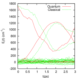
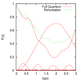
Figure 4: Left: Time evolution of the energy content of the initially excited amide I mode as well as all the remaining modes of $N$-methylacetamide. Quantum (red lines) and classical (green lines) calculations obtained at the DFT/B3LYP level of theory are compared. Right: Comparison of the VCI calculation (red) with the result of the perturbative calculation (green) for the reduced density matrix. [Reprinted with permission from H. Fujisaki, K. Yagi, J.E. Straub, and G. Stock, Int. J. Quant. Chem. 109, 2047 (2009). Copyright ©2009 by Wiley InterScience.]

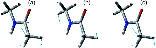
Figure 5: The dominant bath vibrational modes coupled to the amide I mode calculated on the B3LYP/6-31G(d) potential energy surface. [Reprinted with permission from H. Fujisaki, K. Yagi, K. Hirao, and J.E. Straub, Chem. Phys. Lett. 443, 6 (2007). Copyright ©2009 by Elsevier.]

IV.1.2 $N$-methylacetamide/Water cluster

We next examine a somewhat larger system, NMA in a water cluster ZFS09b , an interesting and important model system for exploring the response of amide vibrational modes to “solvation” Skinnergroup . The system size allows for an ab initio quantum mechanical treatment of the potential surface at a higher level of theory, B3LYP/aug-cc-pvdz, relative to the commonly employed B3LYP/6-31G(d). The enhancement in level of theory significantly improves the quality of the NMA-water interaction, specifically the structure and energetics of hydrogen bonding. Since there are at most three hydrogen bonding sites in NMA, it is natural to configure three water molecules around NMA as a minimal model of “full solvation.” NMA-water hydrogen bonding causes the frequency of the amide I mode to red-shift. As a result, the anharmonic coupling between the relaxing mode and the other bath modes will change relative to the case of the isolated NMA. Nevertheless, we observe that the VER time scale remains sub ps as is the case for isolated NMA (Fig. 6). Though there are intermolecular (NMA-water) contributions to VER, they do not significantly alter the VER timescale. Another important finding is that the energy pathway from the amide I to amide II mode is “open” for the NMA-water cluster system. This result is in agreement with experimental results by Tokmakoff and coworkers Tokmakoff06 and recent theoretical investigation Knoester08 . Comparison between singly (NMA-$d_{1}$) and fully (NMA-$d_{7}$) deuterated cases shows the VER time scale become somewhat longer for the case of NMA-$d_{7}$ (Fig. 6). We also discuss this phenomenon below in the context of the NMA/solvent water system.

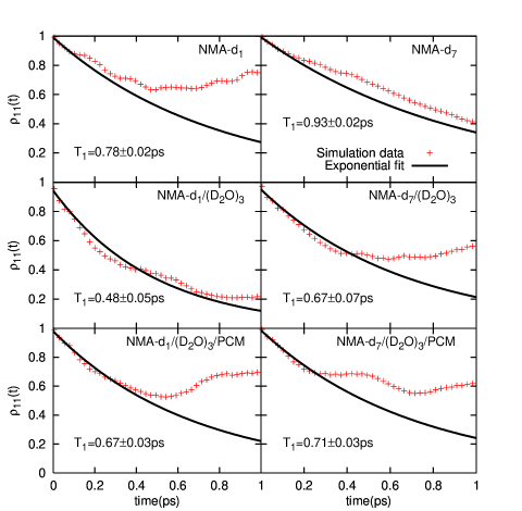
Figure 6: Time evolution of the density matrix for the amide I mode in the NMA-water cluster system after $v=1$ excitation. The derived vibrational energy relaxation time constants $T_{1}$ are also provided. [Reprinted with permission from Y. Zhang, H. Fujisaki, and J.E. Straub, J. Phys. Chem. A 113, 3051 (2009). Copyright ©2009 by the American Chemical Society.]

IV.1.3 $N$-methylacetamide in water solvent

Finally we consider the condensed phase system of NMA in bulk water FZS06 ; FS08 ; SF09 . We attempt to include the full dynamic effect of the system by generating many configurations from molecular dynamics simulations and using them to ensemble-average the results. Note that in the previous examples of isolated NMA and NMA/water clusters, only one configuration at a local minimum of the zero temperature ground state potential surface was used. On the other hand, the potential energy function used is not so accurate as in the previous examples as it is not feasible to include many water molecules at a high level of theory. We have used the CHARMM force field to calculate the potential energy and to carry out molecular dynamics simulations.

All simulations were performed using the CHARMM simulation program package CHARMM and the CHARMM22 all-atom force field CHARMMFF was employed to model the solute NMA-$d_{1}$ and the TIP3P water model TIP3P with doubled hydrogen masses to model the solvent D₂O. We also performed simulations for fully deuterated NMA-$d_{7}$. The peptide was placed in a periodic cubic box of (25.5 Å)³ containing 551 D₂O molecules. All bonds containing hydrogens were constrained using the SHAKE algorithm SHAKE . We used a 10 Å  cutoff with a switching function for the nonbonded interaction calculations. After a standard equilibration protocol, we ran a 100 ps NVT trajectory at 300 K, from which 100 statistically independent configurations were collected.

We applied the simplest VER formula Eq. (50) FZS06 as shown in Fig. 7. We truncated the system including only NMA and several water molecules around NMA with a cutoff distance, taken to be 10 Å. For reasons of computational feasibility, we only calculated the normal modes and anharmonic coupling elements within this subsystem.

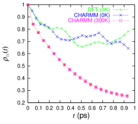
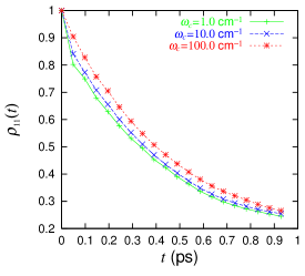
Figure 7: Left: Comparison of the calculation of the $\rho_{11}$ element of the reduced density matrix at different levels of theory. Right: Calculation of the density matrix with different cutoff frequencies. [Reprinted with permission from H. Fujisaki, Y. Zhang, and J.E. Straub, J. Chem. Phys. 124, 144910 (2006). Copyright ©2009 by the American Institute of Physics.]

A number of important conclusions were drawn from these calculations.
(1) The inclusion of “many” solvating water molecules induces the irreversible decay of the excess energy as well as the density matrix elements (population). The important observation is that the VER behavior does not severely depend on the cutoff distance (if it is large enough) and the cutoff frequency. The implication is that if we are interested in a localized mode such as the amide I mode in NMA, it is enough to use a NMA/water cluster system to totally describe the initial process of VER. In a subsequent study, Fujisaki and Stock used only 16 water molecules surrounding NMA (hydrated water) and found reasonable results FS08 .
(2) Comparison of the two isolated NMA calculations suggests that the CHARMM force field works well compared with results based on DFT calculations. This suggests that the use of the empirical force field in exploring VER of the amide I mode may be justified.
(3) There is a classical limit of this calculation FZS06 , which predicts a slower VER rate close to Nguyen-Stock’s quasi-classical calculation Stock . This finding was explored further by Stock Stock09 , who derived a novel quantum correction factor based on the reduced model, Eq. (2).

In these calculations, many solvating water configurations were generated using MD simulations. As such, information characterizing dynamic fluctuation in the environment is ignored. Fujisaki and Stock further improved the methodology to calculate VER FS08 by taking into account the dynamic effects of the environment through the incorporation of time-dependent parameters, such as the normal mode frequencies and anharmonic coupling, derived from the MD simulations as shown in Fig. 8. Their method is described in Sec. III.2, and was applied to the same NMA/solvent water system. As we are principally concerned with high frequency modes, and the instantaneous normal mode frequencies can become unphysical, we adopted a partial optimization strategy. We optimized the NMA under the influence of the solvent water at a fixed position. (For a different strategy, see Ref. Yagi09 .) The right side of Fig. 8 shows the numerical result of the optimization procedure. Through partial optimization, the fluctuations of the parameters become milder than the previous calculations that employed instantaneous normal modes.

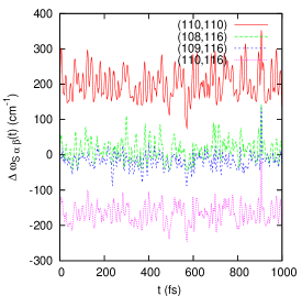
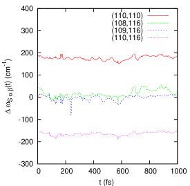
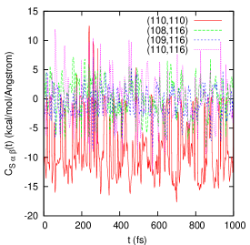
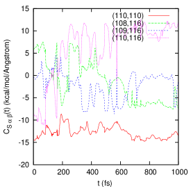
Figure 8: Time evolution of the vibrational dynamics of NMA in D₂O obtained from instantaneous normal mode analysis with (right) and without (left) partial energy minimization. Shown are (upper panels) the frequency mismatch $\Delta\omega_{S\alpha\beta}(t)=\omega_{S}(t)-\omega_{\alpha}(t)-\omega_{\beta}(t)$, for several resonant bath mode combinations, and (lower panels) the corresponding third-order anharmonic couplings, $C_{S\alpha\beta}(t)$. [Reprinted with permission from H. Fujisaki and G. Stock, J. Chem. Phys. 129,134110 (2008). Copyright ©2009 by the American Institute of Physics.]

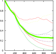
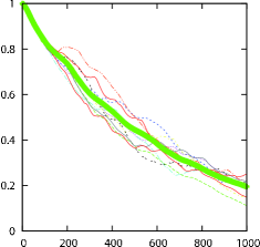
Figure 9: VER calculations of amide I mode population $P(t)$ of NMA with use of instantaneous normal mode analysis and partial energy minimization. Shown are results from (left) the inhomogeneous averaging approximation and (right) dynamical averaging. [Reprinted with permission from H. Fujisaki and G. Stock, J. Chem. Phys. 129,134110 (2008). Copyright ©2009 by the American Institute of Physics.]

The results of numerical calculations based on Eq. (49) are shown in Fig. 9. We see that both partial optimization and dynamical averaging affect the result. The “dynamic” formula, Eq. (49), leads to smaller fluctuations in the results for the density matrix. Apparently, dynamic averaging smoothens the resonant effect, stemming from the frequency difference in the denominator of Eq. (50). For the NMA/solvent water system, the time-averaged value of the Fermi resonance parameter, Eq. (52), can be utilized to clarify the VER pathways as in the case of isolated NMA FS08 . It was shown that the hydrated water (the number of waters is 16) is enough to fully describe the VER process at the initial stage ($\simeq 0.5$ ps). The predictions of the VER rates for the two deuterated cases, NMA-$d_{1}$ and NMA-$d_{7}$, are in good agreement with experiment and also with the NMA/Water cluster calculations ZFS09b . Though the dynamic effect is modest in the case of the NMA/solvent water system, the dynamic formula is recommended when variations of the system parameters due to the fluctuating environment must be taken into account.

IV.2 Cytochrome c in water

The protein, cytochrome c, has been used in experimental and theoretical studies of VER Fujisaki05 ; Straub.JPCB.2003.107.12339 ; Straub.JPCB.2009.113.825 ; Champion.JCP.1992.97.3214 ; Champion.JPCB.2000.104.10789 ; Kruglik.JPCB.2006.110.12766 ; BS03 . Importantly, spectroscopy and simulation have been used to explore the time scales and mechanism of VER of CH stretching modes Fujisaki05 ; BS03 . Here we examine VER of amide I modes in cytochrome c FS07 . Distinct from previous studies Fujisaki05 which (a) employed a static local minimum of the system, we use the dynamical trajectory; (b) in the previous study, the water degrees of freedom were excluded, whereas in this study some hydrating water has been taken into account.

We used the trajectory of cytochrome c in water generated by Bu and Straub BS03 . To study the local nature of the amide I modes and the correspondence with experiment, we isotopically labeled four specific CO bonds, typically C¹²O¹⁶ as C¹⁴O¹⁸. In evaluating the potential energy in our instantaneous normal mode analysis, we truncated the system with an amide I mode at the center using a cutoff ($\simeq 10$ Å), including both protein and water. Following INM analysis, we used Eq. (50) to calculate the time course of the density matrix. The predicted VER is single exponential in character with time scales that are subpicosecond with relatively small variations induced by the different environments of the amide I modes (see Fig. 10 and Table I in FS07 for numerical values of the VER timescales). To identify the principal contributions to the dependence on the environment we examined the VER pathways and the roles played by protein and water degrees of freedom in VER. Our first conclusion is that, for the amide I modes buried in the protein ($\alpha$-helical regions), the water contribution is less than for the amide I modes exposed to water (loop regions). This finding is important because only a total VER timescale is accessible in experiment. With our method, the energy flow pathways into protein or water can be clarified.

Focusing on the resonant bath modes, we analyzed the anisotropy of the energy flow, as shown in Fig. 11, where the relative positions of bath modes participating in VER are projected on the spherical polar coordinates ($\theta,\phi$) centered on the CO bond involved in the amide I mode, which represents the principal z-axis (see Fig. 1 in FS07 ). The angle dependence of the energy flow from the amide I mode to water is calculated from the normal mode amplitude average, and not directly related to experimental observables. As expected, energy flow is observed in the direction of solvating water. However, that distribution is not spatially isotropic and indicates preferential directed energy flow. These calculations demonstrate the power of our theoretical analysis in elucidating pathways for spatially directed energy flow of fundamental importance to studies of energy flow and signaling in biomolecules and the optimal design of nanodevices (see summary and discussion for more detail).

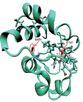
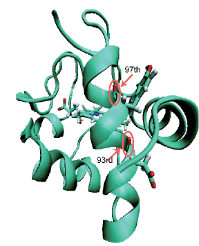
Figure 10: Left: 81st and 84th residues of cytochrome c in a loop region. Right: 93rd and 97th residues of cytochrome c in an $\alpha$ helical region. The cartoon represents the protein using a licorice model to identify the four residues. (The water molecules are excluded for simplicity.) [Reprinted with permission from H. Fujisaki and J.E. Straub, J. Phys. Chem. B 111, 12017 (2007). Copyright ©2009 by the American Chemical Society.]

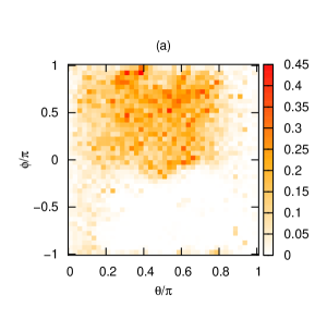
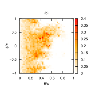
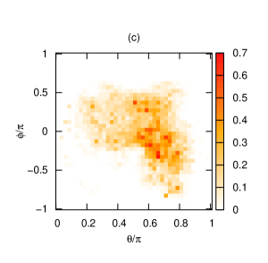
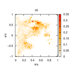
Figure 11: Angular excitation functions for the resonant normal modes of water for the (a) 81st, (b) 84th, (c) 93rd, and (d) 97th residues, represented in arbitrary units. [Reprinted with permission from H. Fujisaki and J.E. Straub, J. Phys. Chem. B 111,12017 (2007). Copyright ©2009 by the American Chemical Society.]

IV.3 Porphyrin

Our final example is a modified porphyrin ZFS09a . We have carried out systematic studies of VER in the porphyrin-imidazole complex, a system that mimics the active site of the heme protein myoglobin (Mb). The structure of myoglobin was first determined in 1958 Kendrew . Experimental and computational studies exploring the dynamics of myoglobin led to the first detailed picture of how fluctuations in a protein structure between a multitude of “conformational substates” supports protein function Frauenfelder . Time resolved spectroscopic studies  Hochstrasser coupled with computational studies have provided a detailed picture of time scale and mechanism for energy flow in myoglobin and its relation to function. Karplus and coworkers developed the CHARMM force field CHARMM for heme and for amino acids for the study of myoglobin, and a particular focus on the dissociation and rebinding of ligands such as CO, NO, and O₂ Mb . The empirical force field appears to provide an accurate model of heme structure and fluctuations. However, we have less confidence in the accuracy of anharmonicity essential to detailed mode coupling on the force field and the dependence on spin state, which is important to the proper identification of the electronic ground state potential energy surface.

We carried out ab initio calculations for a heme-mimicking molecule, iron-porphine ligated to imidazole, abbreviated as FeP-Im. See Fig. 12 for the optimized structure. We employed the UB3LYP/6-31G(d) level of theory as in the case of the isolated NMA FYHS07 ; FYSS09 , but carefully investigated the spin configurations. We identified the quintuplet ($S=2$) as the electronic ground state, in accord with experiment. Our study of VER dynamics on this quintuplet ground state potential energy surface (PES) is summarized here. Additional investigations of the VER dynamics on the PES corresponding to other spin configurations as well as different heme models are described elsewhere ZFS09a .

A series of elegant pioneering experimental studies have provided a detailed picture of the dynamics of the $\nu_{4}$ and $\nu_{7}$ modes, in-plane modes of the heme (see Fig. 13), following ligand photodissociation in myoglobin. Using time-resolved resonance Raman spectroscopy, Mizutani and Kitagawa observed mode specific excitation and relaxation MK97 ; MK01 . Interestingly, these modes decay on different time scales. The VER time scales are $\sim$ 1.0 ps for the $\nu_{4}$ mode and $\sim$ 2.0 ps for the $\nu_{7}$ mode. Using a sub-10-fs pulse, Miller and co-workers extended the range of the coherence spectroscopy up to 3000 cm^-1 Miller2 . The heme $\nu_{7}$ mode was found to be most strongly excited following $Q$ band excitation. By comparing to the deoxyMb spectrum, they demonstrated that the signal was derived from the structural transition from the six-coordinate to the five-coordinate heme. Less prominent excitation of the $\nu_{4}$ mode was also observed. The selective excitation of the $\nu_{7}$ mode, following excitation of out-of-place heme doming, led to the intriguing conjecture that there may be directed energy transfer of the heme excitation to low frequency motions connected to backbone displacement and to protein function. The low frequency heme modes ($<$400 cm^-1) have been studied using femtosecond coherence spectroscopy with a 50 fs pulse Champion . A series of modes at $\sim$40 cm^-1, $\sim$80 cm^-1, $\sim$130 cm^-1 and $\sim$170 cm^-1 were observed for several myoglobin derivatives. The couplings between these modes were suggested. It is a long term goal of our studies to understand, at the mode-specific level, how the flow of excess energy due to ligand dissociation leads to the selective excitation of $\nu_{4}$ and $\nu_{7}$ modes.

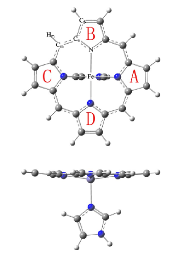
Figure 12: Optimized structure of FeP-Im (quintuplet $S=2$ spin configuration) at the UB3LYP/6-31G(d) level of theory. [Reprinted with permission from Y. Zhang, H. Fujisaki, and J.E. Straub, J. Chem. Phys. 130, 025102 (2009). Copyright ©2009 by the American Institute of Physics.]

In our study, we ignore the transition in spin state that occurs upon ligand photodissociation and the associated electron-nuclear coupling that will no doubt be essential to an understanding of the “initial state” of the $\nu_{4}$ and $\nu_{7}$ vibrations following ligand photodissociation. Our focus was on the less ambitious but important question of vibrational energy flow on the ground state ($S=2$) surface following excitation resulting from photodissociation. We employed time-dependent perturbation theory, Eq. (50), to model the mode-specific relaxation dynamics. The initial decay process of each system mode was fitted by a single-exponential function. The time constant of $\simeq$ 1.7 ps was derived for the $\nu_{4}$ mode and $\simeq$ 2.9 ps for the $\nu_{7}$ mode. These theoretical predictions, which make no assumptions regarding the VER mechanism, agree well with previous experimental results of Mizutani and Kitagawa for MbCO MK97 .

Vibrational energy transfer pathways were identified by calculating the 3rd order Fermi resonance parameters, Eq. (52). For the excited $\nu_{4}$ and $\nu_{7}$ modes, the dominant VER pathways involve porphine out-of-plane motions as energy accepting doorway modes. Importantly, no direct energy transfer between the $\nu_{4}$ and $\nu_{7}$ modes was observed. Cooling of the five Fe-oop (Fe-out-of-plane) modes, including the functionally important heme doming motion and Fe-Im stretching motion, takes place on the picosecond time scale. All modes dissipate vibrational energy through couplings, weaker or stronger, with low frequency out-of-plane modes involving significant imidazole ligand motion. It has been suggested that these couplings trigger the delocalized protein backbone motion, important for protein function, which follows ligand dissociation in Mb.

The $\gamma_{7}$ mode, a porphine methine wagging motion associated with Fe-oop motion, is believed to be directly excited following ligand photodissociation in MbCO. The coupling of this mode to lower frequency bath modes is predicted to be very weak. However, its overtone is strongly coupled to the $\nu_{7}$ mode, forming an effective energy transfer pathway for relaxation on the electronic ground state and excited state surfaces. This strong coupling suggests a possible mechanism of excitation of the $\nu_{7}$ mode through energy transfer from the $\gamma_{7}$ mode. That mechanism is distinctly different from direct excitation together with Fe-oop motion of the $\nu_{4}$ mode and supports earlier conjectures of mode-specific energy transfer following ligand dissociation in myoglobin MK97 ; Miller2 .

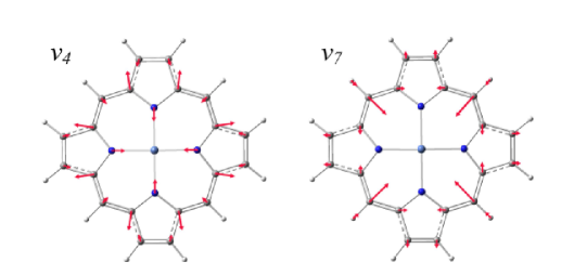
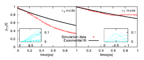
Figure 13: Time course of the $\rho_{11}$ element of the reduced density matrix for $\nu_{4}$ and $\nu_{7}$ excitations of $v=1$. [Reprinted with permission from Y. Zhang, H. Fujisaki, and J.E. Straub, J. Chem. Phys. 130, 025102 (2009). Copyright ©2009 by the American Institute of Physics.]

V Summary and Discussion

This chapter provides an overview of our recent work on the application of the non-Markovian theory of vibrational energy relaxation to a variety of systems of biomolecular interest, including protein backbone mimicking amide I modes in $N$-methylacetamide (in vacuum, in water cluster, and in solvent water) amide I modes in solvated cytochrome c, and vibrational modes in a heme-mimicking porphyrin ligated to imidazole. We calculated the VER time scales and mechanisms using Eq. (49), incorporating a fluctuating bath, and Eq. (50), using a static bath approximation, and compared them to experiment when available. The theory is based on the reduced model using normal mode concepts with 3rd and 4th order anharmonicity, Eq. (2). Applying the simple time-dependent perturbation theory, and ensemble averaging the resulting density matrix, a non-Markovian theory of VER was obtained. We extended the previous theory due to Fujisaki, Zhang and Straub FZS06 to more general situations where (1) the relaxing “system” has a multi-mode character and (2) when the system parameters depend on time FS08 . We also discussed the limitations of our VER formulas related to the assumptions upon which the earlier theories are based.

We are now in a position to discuss the future aspects of our work, and the connection to other biolomolecular systems or nanotechnological devices.

Relation to enzymatic reaction: The role of vibrational motions in the mechanism of enzymatic reactions remains controversial Agarwal . In enzymology, the characterization of the enzymatic reaction rate is essential. Kinetic information is typically derived from substrate-enzyme kinetics experiments. In simulation, the free energy calculation combined with transition state theory is the most powerful and practical way to compute reaction rates. As enzymatically catalyzed reactions typically involve chemical bond breaking and formation, QM/MM type methods should be employed. Warshel and coworkers have examined this issue for several decades, and concluded that characterizing the free energy barrier is the most important consideration, noting that the electrostatic influence from the protein (enzyme) plays a key role Warshel . However, Hammes-Schiffer and coworkers have identified important situations in which VER might play a role in controlling the rate of enzymatic reactions Agarwal . Furthermore, Hynes and coworkers applied the Grote-Hynes theory to the enzymatic reactions, and investigated the dynamic role of the environment PTMHR08 . These recent studies indicate the importance of incorporating vibrational energy flow and dynamics as part of a complete understanding of enzyme kinetics.

Relation to conformational change: The relation between vibrational excitation/relaxation and conformational change of molecules is intriguing in part because of the possible relation to the optimal control of molecular conformational change using tailored laser pulses. It is well known that there are dynamic corrections to the RRKM reaction rate: the simplest being

$$k(E)=k_{RRKM}(E)/(1+\nu_{R}/k_{IVR}(E))$$ (53)

where $\nu_{R}$ is the intrinsic frequency of a reaction coordinate, $k_{IVR}(E)$ is a microcanonical IVR rate, and $k_{RRKM}(E)$ is the RRKM reaction rate Steinfeldbook ; Billingbook ; BBS88 . Several modifications to this formula are summarized in Leitner . It is obvious that VER affects how a molecule changes its shape. However, this is a “passive” role of VER. Combining RRKM theory and the local random matrix theory LW97 , Leitner, Wales and coworkers theoretically studied the active role of vibrational excitations on conformational change of a peptide-like molecule (called NATMA) ALEW05 . There are two particular modes (NH stretching) in NATMA, and they found that the final product depends on which vibrational mode is excited DLWZ04 . For the same system, Teramoto and Komatsuzaki further refined the calculation by employing ab initio potential energy surface TK09 . A possibility to control molecular configurations of peptides or proteins using laser pulses should be pursued and some experimental attempts have begun Hamm08 ; Miller ; Zwier .

Another interesting attempt should be to address mode specific energy flow associated with structural change. Recently Ikeguchi, Kidera, and coworkers IUSK05 developed a linear response theory for conformational changes of biomolecules, which is summarized in another chapter of this volume FMK09 . Though the original formulation is based on a static picture of the linear response theory (susceptibility), its nonequilibrium extension may be used to explore the relation between energy flow and conformational change in proteins. In addition, Koyama and coworkers Koyama08 devised a method based on principal component analysis for individual interaction energies of a peptide (and water), and found an interesting correlation between the principal modes and the direction of conformational change Koyama08 .

Relation to signal transduction in proteins: Though signal transduction in biology mainly denotes the information transfer processes carried out by a series of proteins in a cell, it can be interesting and useful to study the information flow in a single protein, which should be related to vibrational population and phase dynamics. Straub and coworkers Straub studied such energy flow pathways in myoglibin, and found particular pathways from heme to water, later confirmed experimentally by Kitagawa, Mizutani and coworkers KNM06 and Champion and coworkers Champion . Ota and Agard OA05 devised a novel simulation protocol, anisotropic thermal diffusion, and found a partitular energy flow pathway in the PDZ domain protein. Importantly, the pathway they identified is located near the conserved amino acid region in the protein family previously elucidated using information theoretic approach by Lockless and Ranganathan LR99 . Sharp and Skinner SS06 proposed an alternative method, pump-probe MD, and examined the same PDZ domain protein, identifying alternative energy flow pathways. Using linear response theory describing thermal diffusion, Ishikura and Yamato Yamato discussed the energy flow pathways in photoactive yellow protein. This method was recently extended to the frequency domain by Leitner and applied to myoglobin dimer Leitner09b . Though the energy flow mentioned above occurs quite rapidly ($\sim$ ps), there are time-resolved spectroscopic methods to detect these pathways in vitro Hamm08 . Comparison between theory and experiment will help clarify the biological role of such energy flow in biomolecular systems.

Exploring the role of VER in nanodevice design: Applications of the methods described in this chapter are not limited to biomolecular systems. As mentioned in the introduction, heat generation is always an issue in nanotechnology, and an understanding of VER in molecular devices can potentially play an important role in optimal device design. The estimation of thermal conductivity in such devices is a good starting point recently pursued by Leitner Leitner . Nitzan and coworkers studied thermal conduction in a molecular wire using a simplified model SNH03 . It will be interesting to add more molecular detail to such model calculations. Electronic conduction has been one of the main topics in nanotechnology and mesoscopic physics Cuniberti , and heat generation during electronic current flow is an additional related area of importance.

VER in a confined environment: We have found evidence for spatially anisotropic vibrational energy flow with specific pathways determined by resonance and coupling conditions. It was shown for amide I modes in cytochrome c that VER may depend on the position of the probing modes FS07 , making it useful for the study of inhomogeneity of the environment. For example, an experimental study of VER in a reverse micelle environment ZBO03 , fullerene, nanotube, membrane, or on atomic or molecular surfaces Saalfrank may all be approached using methods described in this chapter.

Anharmonic effects in coarse-grained models of proteins: Recently Togashi and Mikhailov studied the conformational relaxation of elastic network models Togashi . Though the model does not explicitly incorporate anharmonicity, small anharmonicity exists, resulting in interesting physical behavior relevant to biological function. Sanejouand and coworkers added explicit anharmonicity into the elastic network models, and studied the energy storage Sanejouand through the lens of “discrete breather” ideas from nonlinear science discrete . Surprisingly, they found that the energy storage may occur in the active sites of proteins. It remains to be seen whether their conjecture will hold for all-atom models of the same system.

- (1) D.M. Leitner and J.E. Straub (editors), Proteins: Energy, Heat and Signal Flow, Taylor and Francis/CRC Press, London (2009).
- (2) A. Nitzan, Chemical Dynamics in Condesed Phase: Relaxation, Transfer, and Reactions in Condensed Molecular Systems, Oxford (2006).
- (3) J.I. Steinfeld, J.S. Francisco, and W.L. Hase, Chemical Kinetics and Dynamics, Prentice-Hall, Inc. (1989).
- (4) G.D. Billing and K.V. Mikkelsen, Introduction to Molecular Dynamics and Chemical Kinetics, John Wiley & Sons (1996).
- (5) B.J. Berne, M. Borkovec and J.E. Straub, J. Phys. Chem. 92, 3711 (1988).
- (6) J.J. Ruiz-Pernia, I. Tunon, V. Moliner, J.T. Hynes, and M. Roca, J. Am. Chem. Soc. 130, 7477 (2008).
- (7) D.M. Leitner and P.G. Wolynes, Chem. Phys. Lett. 280, 411 (1997); S. Northrup and J.T. Hynes, J. Chem. Phys. 73, 2700 (1980).
- (8) D.W. Oxtoby, Adv. Chem. Phys. 40, 1 (1979); ibid. 47, 487 (1981); Ann. Rev. Phys. Chem. 32, 77 (1981); V.M. Kenkre, A. Tokmakoff, and M.D. Fayer, J. Chem. Phys. 101, 10618 (1994).
- (9) R. Rey, K.B. Moller, and J.T. Hynes, Chem. Rev. 104, 1915 (2004); K.B. Moller, R. Rey, and J.T. Hynes, J. Phys. Chem. A 108, 1275 (2004).
- (10) C.P. Lawrence and J. L. Skinner, J. Chem. Phys. 117, 5827 (2002); ibid. 117, 8847 (2002); ibid. 118, 264 (2003); A. Piryatinski, C.P. Lawrence, and J.L. Skinner, ibid. 118, 9664 (2003); ibid. 118, 9672 (2003); C.P. Lawrence and J.L. Skinner, ibid. 119, 1623 (2003); ibid. 119, 3840 (2003).
- (11) S. Okazaki, Adv. Chem. Phys. 118, 191 (2001); M. Shiga and S. Okazaki, J. Chem. Phys. 109, 3542 (1998); ibid. 111, 5390 (1999); T. Mikami, M. Shiga and S. Okazaki, ibid. 115, 9797 (2001); T. Terashima, M. Shiga, and S. Okazaki, ibid. 114, 5663 (2001); T. Mikami and S. Okazaki, ibid. 119, 4790 (2003); T. Mikami and S. Okazaki, ibid. 121, 10052 (2004); M. Sato and S. Okazaki, ibid. 123, 124508 (2005); M. Sato and S. Okazaki, ibid. 123, 124509 (2005).
- (12) D.M. Leitner, Adv. Chem. Phys. 130B, 205 (2005); D.M. Leitner, Phys. Rev. Lett. 87, 188102 (2001); X. Yu and D.M. Leitner, J. Chem. Phys. 119, 12673 (2003); X. Yu and D.M. Leitner, J. Phys. Chem. B 107, 1689 (2003); D.M. Leitner, M. Havenith, and M. Gruebele, Int. Rev. Phys. Chem. 25, 553 (2006); D.M. Leitner, Ann. Rev. Phys. Chem. 59, 233 (2008).
- (13) D.M. Leitner, Y. Matsunaga, C.B. Li, T. Komatsuzaki, R.S. Berry, and M. Toda, Adv. Chem. Phys. in this volume.
- (14) V. Pouthier, J. Chem. Phys. 128, 065101 (2008); V. Pouthier and Y.O. Tsybin, ibid. 129, 095106 (2008); V. Pouthier, Phys. Rev. E 78, 061909 (2008).
- (15) A.G. Dijkstra, T. la Cour Jansen, R. Bloem, and J. Knoester, J. Chem. Phys. 127, 194505 (2007).
- (16) R. Bloem, A.G. Dijkstra, T. la Cour Jansen, and J. Knoester, J. Chem. Phys. 129 055101 (2008).
- (17) P. Hamm, M.H. Lim, R.M. Hochstrasser, J. Phys. Chem. B 102, 6123 (1998); M.T. Zanni, M.C. Asplund, R.M. Hochstrasser, J. Chem. Phys. 114, 4579 (2001).
- (18) Y. Mizutani and T. Kitagawa, Science 278, 443 (1997).
- (19) A. Pakoulev, Z. Wang, Y. Pang, and D.D. Dlott, Chem. Phys. Lett. 380, 404 (2003); Y. Fang, S. Shigeto, N.H. Seong, and D.D. Dlott, J. Phys. Chem. A 113, 75 (2009).
- (20) P. Hamm, J. Helbing, J. Bredenbeck, Ann. Rev. Phys. Chem. 59, 291 (2008).
- (21) H. Fujisaki, L. Bu, and J.E. Straub, Adv. Chem. Phys. 130B, 179 (2005); H. Fujisaki and J.E. Straub, Proc. Natl. Acad. Sci. USA 102, 6726 (2005); M. Cremeens, H. Fujisaki, Y. Zhang, J. Zimmermann, L.B. Sagle, S. Matsuda, P.E. Dawson, J.E. Straub, and F.E.Romesberg, J. Am. Chem. Soc. 128, 6028 (2006).
- (22) H. Fujisaki, Y. Zhang, and J.E. Straub, J. Chem. Phys. 124, 144910 (2006).
- (23) H. Fujisaki and J.E. Straub, J. Phys. Chem. B 111, 12017 (2007).
- (24) B.R. Brooks, R.E. Bruccoleri, B.D. Olafson, D.J. States, S. Swaminathan, and M. Karplus, J. Comp. Chem. 4, 187 (1983); A.D. MacKerell, Jr., B. Brooks, C.L. Brooks, III, L. Nilsson, B. Roux, Y. Won, and M. Karplus, . The Encyclopedia of Computational Chemistry 1. Editors, P.v.R. Schleyer et al. Chichester: John Wiley & Sons, 271-277 (1998); B. R. Brooks, C. L. Brooks III, A. D. Mackerell Jr., L. Nilsson, R. J. Petrella, B. Roux, Y. Won, G. Archontis, C. Bartels, S. Boresch, A. Caflisch, L. Caves, Q. Cui, A. R. Dinner, M. Feig, S. Fischer, J. Gao, M. Hodoscek, W. Im, K. Kuczera, T. Lazaridis, J. Ma, V. Ovchinnikov, E. Paci, R. W. Pastor, C. B. Post, J. Z. Pu, M. Schaefer, B. Tidor, R. M. Venable, H. L. Woodcock, X. Wu, W. Yang, D. M. York, and M. Karplus, J. Comp. Chem. 30, 1545 (2009).
- (25) Gaussian 03, Revision C.02, M. J. Frisch, G. W. Trucks, H. B. Schlegel, G. E. Scuseria, M. A. Robb, J. R. Cheeseman, J. A. Montgomery, Jr., T. Vreven, K. N. Kudin, J. C. Burant, J. M. Millam, S. S. Iyengar, J. Tomasi, V. Barone, B. Mennucci, M. Cossi, G. Scalmani, N. Rega, G. A. Petersson, H. Nakatsuji, M. Hada, M. Ehara, K. Toyota, R. Fukuda, J. Hasegawa, M. Ishida, T. Nakajima, Y. Honda, O. Kitao, H. Nakai, M. Klene, X. Li, J. E. Knox, H. P. Hratchian, J. B. Cross, V. Bakken, C. Adamo, J. Jaramillo, R. Gomperts, R. E. Stratmann, O. Yazyev, A. J. Austin, R. Cammi, C. Pomelli, J. W. Ochterski, P. Y. Ayala, K. Morokuma, G. A. Voth, P. Salvador, J. J. Dannenberg, V. G. Zakrzewski, S. Dapprich, A. D. Daniels, M. C. Strain, O. Farkas, D. K. Malick, A. D. Rabuck, K. Raghavachari, J. B. Foresman, J. V. Ortiz, Q. Cui, A. G. Baboul, S. Clifford, J. Cioslowski, B. B. Stefanov, G. Liu, A. Liashenko, P. Piskorz, I. Komaromi, R. L. Martin, D. J. Fox, T. Keith, M. A. Al-Laham, C. Y. Peng, A. Nanayakkara, M. Challacombe, P. M. W. Gill, B. Johnson, W. Chen, M. W. Wong, C. Gonzalez, and J. A. Pople, Gaussian, Inc., Wallingford CT, 2004.
- (26) E. B. Wilson, Jr., J.C. Decius, and P.C. Cross, Molecular Vibrations, Dover (1980).
- (27) Q. Cui and I. Bahar (editors), Normal Mode Analysis: Theory and Applications to Biological and Chemical Systems, Chapman & Hall/CRC Press, London (2006).
- (28) N. Go, T. Noguchi, and T. Nishikawa, Proc. Natl. Acad. Sci. USA 80, 3696 (1983); B. Brooks and M. Karplus, ibid. 80, 6571 (1983).
- (29) D. van der Spoel, E. Lindahl, B. Hess, G. Groenhof, A. E. Mark and H. J. C. Berendsen, J. Comp. Chem. 26, 1701 (2005).
- (30) D.A. Case, T.E. Cheatham, III, T. Darden, H. Gohlke, R. Luo, K.M. Merz, Jr., A. Onufriev, C. Simmerling, B. Wang, and R. Woods, J. Comp. Chem. 26, 1668 (2005).
- (31) H. Wako, S. Endo, K. Nagayama, and N. Go, Comp. Phys. Comm. 91, 233 (1995).
- (32) F. Tama, F.-X. Gadea, O. Marques, and Y.-H. Sanejouand, Proteins, 41, 1 (2000).
- (33) L. Mouawad and D. Perahia, Biopolymers, 33, 569 (1993).
- (34) M.M. Tirion, Phys. Rev. Lett. 77, 1905 (1996).
- (35) T. Haliloglu, I. Bahar, and B. Erman, Phys. Rev. Lett. 79, 3090 (1997).
- (36) M. Cho, G.R. Fleming, S. Saito, I. Ohmine, and R.M. Stratt, J. Chem. Phys. 100, 6672 (1994); J.E. Straub and J.-K. Choi, J. Phys. Chem. 98, 10978-10987 (1994); R.M. Stratt Acc. Chem. Res. 28, 201 (1995); T. Keyes, J. Phys. Chem. A 101, 2921 (1997);
- (37) S. Fuchigami, Y. Matsunaga, H. Fujisaki, and A. Kidera, Adv. Chem. Phys. in this volume.
- (38) K. Moritsugu, O. Miyashita and A. Kidera, Phys. Rev. Lett. 85, 3970, (2000); J. Phys. Chem. B 107, 3309 (2003).
- (39) M. Toda, R. Kubo, and N. Saito, Statistical Physics I: Equilibrium Statistical Mechanics, Springer, 2nd edition (2004).
- (40) I. Okazaki, Y. Hara, and M. Nagaoka, Chem. Phys. Lett. 337, 151 (2001); M. Takayanagi, H.Okumura, and M.Nagaoka, J. Phys. Chem. B 111, 864 (2007).
- (41) D. E. Sagnella and J. E. Straub, J. Phys. Chem. B 105, 7057 (2001); L. Bu and J. E. Straub, ibid. 107, 10634 (2003); L. Bu and J. E. Straub, ibid. 107, 12339 (2003); Y. Zhang, H. Fujisaki, and J. E. Straub, ibid. 111, 3243 (2007); Y. Zhang and J.E. Straub, ibid. 113, 825 (2009).
- (42) P.H. Nguyen and G. Stock, J. Chem. Phys. 119, 11350 (2003); P. H. Nguyen and G. Stock, Chem. Phys. 323, 36 (2006); P. H. Nguyen, R. D. Gorbunov, and G. Stock, Biophys. J. 91, 1224 (2006); E. Backus, P.H. Nguyen, V. Botan, R. Pfister, A. Moretto, M. Crisma, C. Toniolo, O. Zerbe, G. Stock, and P. Hamm J. Phys. Chem. B 112, 15487 (2008); P.H. Nguyen, P. Derreumaux and G. Stock, J. Phys. Chem. B 113, 9340-9347 (2009).
- (43) X. Yu and D.M. Leitner, J. Chem. Phys. 119, 12673 (2003); D.A. Lidar, D. Thirumalai, R. Elber, and R.B. Gerber, Phys. Rev. E 59, 2231 (1999).
- (44) A. Roitberg, R.B. Gerber, R. Elber, and M.A. Ratner, Science, 268, 1319 (1995).
- (45) K. Yagi, S. Hirata, and K. Hirao, Theo. Chem. Acc. 118, 681 (2007); K. Yagi, S. Hirata, and K. Hirao, Phys. Chem. Chem. Phys. 10, 1781-1788 (2008).
- (46) K. Yagi, H. Karasawa, S. Hirata, and K. Hirao, ChemPhysChem 10, 1442-1444 (2009).
- (47) H. Fujisaki and G. Stock, J. Chem. Phys. 129, 134110 (2008).
- (48) S. Carter, S.J. Culik, and J.M. Bowman, J. Chem. Phys. 107, 10458 (1997); S. Carter and J.M. Bowman, J. Chem. Phys. 108, 4397 (1998).
- (49) S. Carter, J.M. Bowman, and N.C. Handy, Theor. Chem. Acc. 100, 191 (1998).
- (50) K. Yagi, SINDO Version 1.3, 2006.
- (51) H. J. Bakker, J. Chem. Phys. 121, 10088 (2004).
- (52) E.L. Sibert and R. Rey, J. Chem. Phys. 116, 237 (2002); T.S. Gulmen and E.L. Sibert, J. Phys. Chem. A 109, 5777 (2005); S.G. Ramesh and E.L. Sibert, J. Chem. Phys. 125 244512 (2006); S.G. Ramesh and E.L. Sibert, ibid. 125 244513 (2006).
- (53) M. Gruebele and P.G. Wolynes, Acc. Chem. Res. 37, 261 (2004); M. Gruebele, J. Phys.: Condens. Matter 16, R1057 (2004).
- (54) J.S. Bader and B.J. Berne, J. Chem. Phys. 100, 8359 (1994).
- (55) Q. Shi and E. Geva, J. Chem. Phys. 118, 7562 (2003); Q. Shi and E. Geva, J. Phys. Chem. A 107, 9059 (2003); Q. Shi and E. Geva, ibid. 107, 9070 (2003); B.J. Ka, Q. Shi, and E. Geva, ibid. 109, 5527 (2005); B.J. Ka and E. Geva, ibid. 110, 13131 (2006); I. Navrotskaya and E. Geva, ibid. 111, 460 (2007); I. Navrotskaya and E. Geva, J. Chem. Phys. 127, 054504 (2007).
- (56) B.J. Berne and D. Thirumalai, Ann. Rev. Phys. Chem. 37, 401 (1986); G. Krilov, E. Sim, and B.J. Berne, Chem. Phys. 268, 21 (2001).
- (57) S.K. Gregurick, G.M. Chaban, and R.B. Gerber, J. Phys. Chem. A 106, 8696 (2002).
- (58) M. Shiga, M. Tachikawa, and H. Fujisaki, unpublished.
- (59) S. Krimm and J. Bandekar, Adv. Prot. Chem. 38, 181 (1986); A. Barth and C. Zscherp, Q. Rev. Biophys. 35, 369 (2002).
- (60) H. Torii and M. Tasumi, J. Chem. Phys. 96, 3379 (1992).
- (61) H. Torii and M. Tasumi, J. Raman Spec. 29, 81 (1998); H. Torii, J. Phys. Chem. B 111, 5434 (2007); H. Torii, ibid. 112, 8737 (2008).
- (62) S. A. Corcelli, C. P. Lawrence, and J. L. Skinner, J. Chem. Phys. 120, 8107 (2004); Schmidt, J.R.; Corcelli, S.A.; Skinner, J.L. ibid. 121, 8887 (2004); S. Li, J. R. Schmidt, S. A. Corcelli, C. P. Lawrence, and J. L. Skinner, ibid. 124, 204110 (2006).
- (63) S. Ham, S. Hahn, C. Lee, and M. Cho, J. Phys. Chem. B 109, 11789 (2005); M. Cho, Chem. Rev. 108, 1331 (2008); Y.S. Kim and R.M. Hochstrasser, J. Phys. Chem. B 113, 8231 (2009).
- (64) W. Zhuang, D. Abramavicius, T. Hayashi, and S. Mukamel, J. Phys. Chem. B 110, 3362 (2003); T. Hayashi, T.l.C. Jansen, W. Zhuang, and S. Mukamel, J. Phys. Chem. A 64, 109 (2005); T. Hayashi, and S. Mukamel J. Phys. Chem. B, 111, 11032 (2007); T. Hayashi and S. Mukamel, J. Mol. Liq. 141, 149 (2008).
- (65) R.D. Gorbunov, P.H. Nguyen, M. Kobus, and G. Stock,. J. Chem. Phys. 126, 054509 (2007); R.D. Gorbunov and G. Stock, Chem. Phys. Lett. 437, 272 (2007); M. Kobus, R.D. Gorbunov, P.H. Nguyen, and G. Stock,. Chem. Phys. 347, 208 (2008).
- (66) H. Fujisaki, K. Yagi, K. Hirao, and J.E. Straub, Chem. Phys. Lett. 443, 6 (2007).
- (67) H. Fujisaki, K. Yagi, J.E. Straub, and G. Stock, Int. J. Quant. Chem. 109, 2047 (2009).
- (68) S. Ataka, H. Takeuchi, and M. Tasumi, J. Mol. Struct. 113, 147 (1984).
- (69) M. Bounouar and Ch. Scheurer, Chem. Phys. 323, 87 (2006).
- (70) A.L. Kaledin and J.M. Bowman, J. Phys. Chem. A 111, 5593 (2007).
- (71) G. Stock and U. Müller, J. Chem. Phys. 111, 65 (1999); U. Müller and G. Stock, ibid. 111, 77 (1999).
- (72) Y. Zhang, H. Fujisaki, and J.E. Straub, J. Phys. Chem. A 113, 3051 (2009).
- (73) G. Rauhut, J. Chem. Phys. 121, 9313 (2004).
- (74) L.P. DeFlores, Z. Ganim, S.F. Ackley, H.S. Chung, and A. Tokmakoff, J. Phys. Chem. B 110, 18973 (2006).
- (75) A.D. MacKerell Jr., D. Bashford, M. Bellott, R.L. Dunbrack, J.D. Evanseck, M.J. Field, S. Fischer, J. Gao, H. Guo, S. Ha, D. Joseph-McCarthy, L. Kuchnir, K. Kuczera, F.T.K. Lau, C. Mattos, S. Michnick, T. Ngo, D.T. Nguyen, B. Prodhom, W.E. Reiher, B. Roux, M. Schlenkrich, J.C. Smith, R. Stote, J.E. Straub, M. Watanabe, J. Wiorkiewicz-Kuczera, D. Yin, and M. Karplus, J. Phys. Chem. B 102, 3586 (1998).
- (76) W.L. Jorgensen, J. Chandrasekhar, J. Madura, R.W. Impey, and M.L. Klein, J. Chem. Phys. 79, 926 (1983).
- (77) J.-P. Ryckaert, G. Ciccotti, and H.J.C. Berendsen, J. Comp. Phys. 23, 327 (1977).
- (78) G. Stock, Phys. Rev. Lett. 102, 118301 (2009).
- (79) K. Yagi and D. Watanabe, Int. J. Quant. Chem. 109, 2080 (2009).
- (80) L. Bu and J.E. Straub, J. Phys. Chem. B 107, 12339 (2003).
- (81) Y. Zhang and J.E. Straub, J. Phys. Chem. B 113, 825, (2009).
- (82) P. Li, J.T. Sage and P.M. Champion, J. Chem. Phys. 97, 3214 (1992).
- (83) W. Wang, X. Ye, A.A. Demidov, F. Rosca, T. Sjodin, W. Cao, M. Sheeran and P.M. Champion, J. Phys. Chem. B 104, 10789 (2000).
- (84) M. Negrerie, S. Cianetti, M.H. Vos, J. Martin and S.G. Kruglik, J. Phys. Chem. B 110, 12766 (2006).
- (85) L. Bu and J.E. Straub, Biophys. J. 85, 1429 (2003).
- (86) Y. Zhang, H. Fujisaki, and J.E. Straub, J. Chem. Phys. 130, 025102 (2009); Y. Zhang and J.E. Straub, ibid. 130, 095102 (2009); ibid. 130, 215101 (2009).
- (87) J.C. Kendrew, G. Bodo, H.M. Dintzis, R.G. Parrish, H. Wyckoff, and D.C. Phillips, Nature 181, 662 (1958).
- (88) H. Frauenfelder, S.G. Sligar, and P.G. Wolynes, Science 254, 1598 (1991).
- (89) Y. Mizutani and T. Kitagawa, Chem. Rec. 1, 258 (2001); M.H. Vos, Biochim. Biophys. Acta 1777, 15 (2008).
- (90) J.E. Straub and M. Karplus, Chem. Phys. 158, 221 (1991); M. Meuwly, O.M. Becker, R. Stote and M. Karplus, Biophys. Chem. 98, 183 (2002); R. Elber and Q.H. Gibson, J. Phys. Chem. B 112, 6147 (2008).
- (91) M.R. Armstrong, J.P. Ogilvie, M.L. Cowan, A.M. Nagy and R.J.D. Miller, Proc. Natl. Acad. Sci. U.S.A. 100, 4990 (2003); A.M. Nagy, V. Raicu and R.J.D. Miller, Biochimica et Biophysica Acta 1749, 148 (2005).
- (92) F. Rosca, A.T.N. Kumar, X. Ye, T. Sjodin, A.A. Demidov and P.M. Champion, J. Phys. Chem. A 104, 4280 (2000); F. Rosca, A.T.N. Kumar, D. Ionascu, T. Sjodin, A.A. Demidov and P.M. Champion, J. Chem. Phys. 114, 10884 (2001); F. Rosca, A.T.N. Kumar, D. Ionascu, X. Ye, A.A. Demidov, T. Sjodin, D. Wharton, D. Barrick, S.G. Sligar, T. Yonetani and P.M. Champion, J. Phys. Chem. A 106, 3540 (2002); P.M. Champion, F. Rosca, D. Ionascu, W. Cao and X. Ye, Faraday Discuss. 127, 123 (2004); F. Gruia, X. Ye, D. Ionascu, M. Kubo, and P.M. Champion, Biophys. J. 93, 4404 (2007); F. Gruia, M. Kubo, X. Ye, D. Lonascu, C. Lu, R.K. Poole, S. Yeh, and P.M. Champion, J. Am. Chem. Soc. 130, 5231 (2008).
- (93) P.K. Agarwal, S.R. Billeter, P.R. Rajagopalan, S.J. Benkovic, and S. Hammes-Schiffer, Proc. Natl. Acad. Sci. USA 301, 2794 (2002); P. Agarwal, J. Am. Chem. Soc. 127, 15248 (2005); A. Jiménez, P. Clapés, and R. Crehuet, J. Mol. Model 14, 735 (2008).
- (94) A. Warshel and W.W. Parson, Q. Rev. Biophys. 34, 563 (2001).
- (95) J.K. Agbo, D.M. Leitner, D.A. Evans, and D.J. Wales, J. Chem. Phys. 123, 124304 (2005).
- (96) B C. Dian, A. Longarte, P.R. Winter, and T.S. Zwier, J. Chem. Phys. 120, 133 (2004).
- (97) H. Teramoto and T. Komatsuzaki, unpublished.
- (98) A. Nagy, V. Prokhorenko, and R.J.D. Miller, Curr. Opin. Struct. Biol. 16, 654 (2006).
- (99) T.S. Zwier, J. Phys. Chem. A 110, 4133-4150 (2006).
- (100) M. Ikeguchi, J. Ueno, M. Sato, and A. Kidera, Phys. Rev. Lett. 94, 078102 (2005); S. Omori, S. Fuchigami, M. Ikeguchi, and A. Kidera, J. Comp. Chem. (in press), DOI 10.1002/jcc.21269.
- (101) Y.M. Koyama, T.J. Kobayashi, S. Tomoda, and H.R. Ueda, Phys. Rev. E 78, 046702 (2008).
- (102) Y. Gao, M. Koyama, S.F. El-Mashtoly, T. Hayashi, K. Harada, Y. Mizutani, and T. Kitagawa, Chem. Phys. Lett. 429, 239 (2006); M. Koyama, S. Neya, and Y. Mizutani, ibid. 430, 404 (2006).
- (103) N. Ota and D.A. Agard, J. Mol. Biol. 351, 345 (2005).
- (104) S.W. Lockless and R. Ranganathan, Science 286, 295 (1999).
- (105) K. Sharp and J.J. Skinner, Proteins, 65, 347 (2006).
- (106) T. Ishikura and T. Yamato, Chem. Phys. Lett. 432, 533 (2006).
- (107) D.M. Leitner, J. Chem. Phys. 130, 195101 (2009).
- (108) D. Segal, A. Nitzan, and P. Hänggi, J. Chem. Phys. 119, 6840 (2003).
- (109) M. del Valle, R. Gutierrez-Laliga, C. Tejedor, and G. Cuniberti, Nature Nano. 2, 176 (2007); T. Yuge and A. Shimizu, J. Phys. Soc. Jpn. 78, 083001 (2009).
- (110) Q. Zhong, A.P. Baronavski, and J.C. Owrutsky, J. Chem. Phys. 118, 7074 (2003).
- (111) P. Saalfrank, Chem. Rev. 106, 4116 (2006).
- (112) Y. Togashi and A.S. Mikhailov, Proc. Natl. Acad. Sci. USA 104, 8697– 8702 (2007).
- (113) B. Juanico, Y.H. Sanejouand, F. Piazza, and P. De Los Rios, Phys. Rev. Lett. 99, 238104 (2007).
- (114) G. Kopidakis, S. Aubry, and G.P. Tsironis, Phys. Rev. Lett. 87, 165501 (2001).