Evolution of the synchrotron and inverse Compton emission of the low energy peaked BL Lac object S5 0716+714

Abstract

This paper presents a detailed analysis of temporal and spectral variability of the low energy peaked BL Lac object S5 0716+714 with a long ($\sim 74$ ks) X-ray observation performed by XMM-Newton on 2007 September 24–25. The source experiences recurrent flares on timescales of hours. The soft X-ray variations, up to a factor of $\sim 4$, are much stronger than the hard X-ray variations. With higher energy, the variability amplitude increases in the soft X-rays but decreases in the hard X-rays. The hard X-ray variability amplitude, however, is effectively large. For the first time, we detect a soft lag of $\sim 1000$ s between the soft and hard X-ray variations. The soft lags might become larger with larger energy differences. The overall X-ray spectra exhibit a softer-when-brighter trend, whereas the soft X-ray spectra appear to show a harder-when-brighter trend. The concave X-ray spectra of the source can be interpreted as the sum of the high energy tail of the synchrotron emission, dominating in the soft X-rays, and the low energy end of the inverse Compton (IC) emission, contributing more in the hard X-rays. The synchrotron spectra are steep ($\Gamma\sim 2.6$), while the IC spectra are flat ($\Gamma\sim 1.2$). The synchrotron spectra appear to harden with larger synchrotron fluxes, while the IC spectra seem to soften with larger IC fluxes. When the source brightens, the synchrotron fluxes increase but the IC fluxes decrease. The synchrotron tail exhibits larger flux variations but smaller spectral changes than the IC component does. The crossing energies between the two components and the trough energies of spectral energy distributions (SEDs) increase when the source brightens. The X-ray spectral variability demonstrates that the synchrotron and IC SED peaks of S5 0716+714 shift to higher energies when it brightens. The temporal variability also elucidates that the hard X-ray variations of the source might be dominated by the synchrotron tail. The simultaneous optical and UV data obtained with XMM-Newton are compared with the X-ray observations.

1 Introduction

Blazars, an assembly of BL Lac objects and flat spectrum radio quasars (FSRQs), are the most extreme class of Active Galactic Nuclei (AGN). They are remarkably characterized by variability of different amplitude on various timescales across most of the electromagnetic wavelengths (e.g., Ulrich et al. 1997). The radiation from blazars is thought to originate in a relativistic jet closely aligned with the line of sight, which is thus relativistically beamed (e.g., Urry & Padovani 1995). In the $\log(\nu F_{\nu})-\log(\nu)$ representation, the spectral energy distributions (SEDs) of blazars comprise of two broad bumps. The low energy bump peaks at the frequencies ranging from sub-millimeter to X-ray bands, while the peak of the high energy bump is thought to be at the MeV-TeV gamma-ray bands though it has not been well-known for most of blazars yet. The low energy component is widely believed to be the synchrotron emission of a relativistic electron population residing in the jet tangled with magnetic field, whereas the high energy component is thought to be the Inverse Compton (IC) radiation of the same electron population, scattering the low energy photons of either its own synchrotron photons (the synchrotron self-Compton [SSC, e.g., Maraschi et al. 1992] model mostly adopted for BL Lac objects) or the external photons of surrounding environment (the External Compton [EC, e.g., Sikora et al. 1994] model mostly used for FSRQs).

The current classification of blazars is preferably based on the peak energy of the synchrotron emission component. BL Lac objects are differentiated into high energy peaked BL Lac objects (HBLs) and low energy-peaked BL Lac objects (LBLs) (Giommi & Padovani 1994; Padovani & Giommi 1995). The synchrotron emission of HBLs and LBLs peaks at the UV/X-ray and the IR-optical wavelengths, respectively. The synchrotron peak of FSRQs might shift down to lower (e.g., sub-millimeter) frequencies. The location of the synchrotron peak is thought to be related with the bolometric luminosity of the source: the higher the luminosity, the lower the peak energy (Fossati et al. 1998; Ghisellini et al. 1998). This is the so-called blazar SED sequence widely cited in the blazar studies. Historically, LBLs and HBLs are best observed and studied in the optical and X-ray bands, respectively, because LBLs are usually the brightest and most variable objects in the optical wavelengths, whereas HBLs are the brightest and most variable ones in the X-rays. The optical variability properties of the LBL BL Lacertae are analogous to the X-ray variability properties of bright HBLs (Papadakis et al. 2003; Bian et al. 2007). This similarity is anticipated, since the optical emission of LBLs and the X-ray emission of HBLs correspond to the synchrotron peak of their own, respectively. Because it originates in a different dominance of the synchrotron over the IC radiation, the X-ray emission of different classes of blazars shows very different characteristics of temporal and spectral variability (see Pian 2002 and Zhang 2003 for reviews).

HBLs are bright and best studied X-ray sources. Their X-ray emission is commonly interpreted as the synchrotron radiation from the high-energy tail of an electron distribution, which is sensitive to the particle acceleration and cooling and thus shows rapid and strong variability (e.g., Kirk et al. 1998). Repeated X-ray observations have been performed for a few X-ray bright HBLs with various X-ray telescopes. Although it is complicated, the temporal and spectral variability of HBLs might be characterized as follows. The X-ray fluxes of HBLs exhibit large amplitude variability on different timescales. Rapid variations are common, e.g., the fluxes of PKS 2155–304 changed by a factor of $\sim 2$ on timescales of the order of a few hours (Sembay et al. 1993; Zhang et al. 1999). The variability amplitude increases with higher energy (Mrk 421: Ravasio et al. 2004; PKS 2155–304: Zhang et al. 2005, 2006b; Mrk 510: Gliozzi et al. 2006), in accordance with the fact that the higher energy electrons have shorter cooling timescales. The X-ray spectra of HBLs are steep ($\Gamma>2$) and show a convex shape. More precisely, the X-ray spectra continuously steepen with energies (e.g., Perman et al. 2005; Tramacere et al. 2007). Flux changes are frequently accompanied by spectral variability. The spectra typically harden with higher fluxes (e.g., Mrk 421: Brinkmann et al. 2005; PKS 2155-304: Sembay et al. 2002), i.e., the so-called harder-when-brighter phenomenon. The synchrotron peaks have been determined to locate in the X-ray band for a few bright HBLs, which shift to higher energies as the source brightens (e.g., Mrk 421: Fossati et al. 2000; Massaro et al. 2004a; Tanihata et al. 2004; Tramacere et al. 2009; Mrk 501: Massaro et al. 2004b). The variations between different energies are well correlated within the X-ray band, often with time lags. The lags, when detected, appear to change from flare to flare (e.g., Mrk 421: Takahashi et al. 2000; PKS 2155–304: Zhang et al. 2002; 2006a). The variations at lower energies often lag behind those at higher energies (soft lag), although the opposite behavior (hard lag) has been also claimed (Mrk 421: Zhang 2002; Ravasio et al. 2004; Brinkmann et al. 2003; PKS 2155–305: Zhang et al. 2006a; 1ES 1218+304: Sato et al. 2008). With the XMM-Newton PN timing mode X-ray observations of Mrk 421, Brinkmann et al. (2005) claimed that both the sign and the length of lags may change on timescales of a few thousand seconds. The lags are also energy dependent, increasing with larger energy differences (e.g., Mrk 421: Takahashi et al. 1996; Zhang 2002; Zhang et al. 2010; PKS 2155–304: Kataoka et al. 2000; Zhang et al. 2002). Spectral variability may correspond to the existence of the inter-band time lags. Spectral evolution with flux has been systematically resolved for some well-defined flares. On the spectral index–flux ($\alpha-F$) plot, clockwise and counter-clockwise loops have been effectively observed to correspond to the soft and hard lag (e.g., Mrk 421: Takahashi et al. 1996; Zhang 2002, 2010; Ravasio et al. 2004; PKS 2155–304: Kataoka et al. 2000; Zhang et al. 2002), respectively. The sign of the lags and the pattern of the loops have been thought to be the results of the balance between the acceleration and cooling timescales of the electron population responsible for the observed X-ray emission (Kirk et al. 1998; Zhang et al. 2002). This in turn has been used to constrain some of the physical parameters (the magnetic field and the Doppler factor) of the emitting region.

The X-ray spectra of LBLs have a concave shape with a break energy of $\sim 2$ keV, which has been clearly detected in a few bright objects with the synchrotron emission peaking in the optical band (e.g., BL Lacertae: Tanihata et al. 2000; Ravasio et al. 2002, 2003; S5 0716+714: Wagner et al. 1996; ON 231: Tagliaferri et al. 2000). The spectra are steep ($\Gamma\sim 2.3$) in the soft X-rays, while they are flat ($\Gamma\sim 1.7$) in the hard X-rays. On timescale of hours, the soft X-ray fluxes are highly variable, whereas the hard X-ray fluxes tend to be stable (e.g., Tanihata et al. 2000; Ravasio et al. 2003; Giommi et al. 1999; Tagliaferri et al. 2000). Therefore, LBLs shows different spectral and temporal properties in the soft and hard X-rays, which is thought to be due to different emission components. The soft X-rays are dominated by the synchrotron emission from the high-energy tail of an electron distribution, whereas the IC scattering of the low-energy side of the same electron distribution off the synchrotron (and/or external in some cases) photons contributes more in the hard X-rays (e.g., Giommi et al. 1999). The high energy tail of the synchrotron emission is variable and has a steep spectrum. The low energy side of the IC emission is stable and its spectrum is flat. Accordingly, the studies of LBLs in the X-rays are able to understand the physical conditions of the low- and high-energy electrons simultaneously. By fitting the X-ray spectra with the double power law model, Tanihata et al. (2000) and Ferrero et al. (2006) disentangled the two emission components for BL Lacertae and S5 0716+714. The synchrotron emission is variable on short timescales (e.g., $\sim$ hours), whereas the IC emission appears to vary on longer timescales (e.g., $\sim$ days). The breaking energies become higher with higher fluxes (e.g., BL Lacertae: Ravasio et al. 2003). The overall X-ray spectra show the softer-when-brighter behaviour (e.g., Giommi et al. 1999. These phenomena are ascribed to the upshift of the synchrotron peak to higher energy when the sources brighten. No inter-band time lags or the spectral index–flux loops have been clearly reported so far for LBLs, although they are theoretically expected (B${\rm\ddot{o}}$ttcher & Chiang 2002).

S5 0716+714 is identified as a prototype of LBLs since its synchrotron emission peaks in the optical band (e.g., Nieppola et al. 2006). The photometric detection of its host galaxy suggested a redshift of $0.31\pm 0.08$ (Nilsson et al. 2008). It has been intensively observed and studied in many wavelengths, especially in the optical band (e.g., Wu et al. 2007 and reference therein). It is strongly variable from radio to X-ray bands on different timescales (e.g., Wagner et al. 1996). The EGRET onboard the Compton Gamma-ray Observatory detected its high energy gamma-ray ($>100$ MeV) emission several times from 1991 to 1996 (Hartman et al. 1999). The gamma-ray fluxes varied by a factor of two on timescale of years, but the spectral index–flux correlation was not found (Nandikotkur et al. 2007). In 2008, AGILE detected a variable gamma-ray flux, with a peak flux above the maximum obtained by EGRET (Chen et al. 2008). Observations by HEGRA resulted in an upper limit of flux at very high energy (VHE) gamma-ray energies ($>1.6$ TeV) (Aharonian et al. 2004). It is also in the first Fermi-LAT bright source list (Abdo et al. 2009). Recently, the MAGIC collaboration reported the first detection of VHE gamma-rays from the source at $5.8\sigma$ level (Anderhub et al. 2009). The discovery of S5 0716+714 as a VHE gamma-ray LBL was triggered by its very high optical state, suggesting a possible correlation between the VHE gamma-ray and the optical emissions. S5 0716+714 is also a preferred target to perform simultaneous multi-wavelength observations (e.g., Villata et al. 2008; Giommi et al. 2008). Wu et al. (2009) reported the first detection of time lags between the variations in different optical wavelengths.

S5 0716+71 has been observed by various X-ray telescopes. The observations in 1991 March with the PSPC onboard ROSAT revealed a behavior of flux-related spectral variations in the 0.1–2.4 keV band. Two distinct spectral components are needed to describe the concave X-ray spectra (Cappi et al. 1994). ASCA observed the source in 1994 March and confirmed the spectral shape found by ROSAT in higher energies: the spectra flatten with increasing energies (Kubo et al. 1998). The three BeppoSAX observations in 1996, 1998 and 2000 revealed the spectral and temporal variability of the two spectral components. It was in faint states in the 1996 and 1998 observation (Giommi et al. 1999). The spectral fits with a broken power law model resulted in concave spectra in the 0.1–10 keV band, breaking at $\sim 2-3$ keV. The 2000 observation caught the source in its high state (Tagliaferri et al. 2003). The concave spectra can be disentangled into two power law components, crossing at $\sim 1.5$ keV. The steeper power law component dominates the soft X-ray emission, whereas the flatter one contributes more to the hard X-rays. The soft X-ray spectral index is the largest out of the three BeppoSAX observations, indicating a softer-when-brighter behaviour for the soft X-ray variability. The BeppoSAX observations also revealed large and rapid variations in the soft X-ray band and the lack of variations above $\sim 3$ keV. In the 1996 observation, a flare with duration of $\sim 20$ hours was detected in the soft but not in the hard X-ray band (Giommi et al. 1999). Variations by a factor of $\sim 3$ on a timescale of one hour was detected below $\sim 3$ keV and no variations above (Tagliaferri et al. 2003). Nevertheless, the comparisons between the three observations show that the hard X-ray fluxes were also variable over the timescales of years. The temporal and spectral variability of S5 0716+714 is in good agreement with the interpretation that the soft and hard X-ray emission, separating at $\sim 2-3$ keV, are dominated by the strongly variable high energy tail of the synchrotron radiation and the ”stable” low energy side of the IC radiation, respectively. The softer-when-brighter behaviour, opposite to the harder-when-brighter one frequently observed in HBLs, could be ascribed by the upshift of the synchrotron peak to higher energy as the source brightens, causing the synchrotron tail to enter into the soft X-ray band more (e.g., Giommi et al. 1999).

However, previous X-ray observations were not able to disentangle the two spectral components and related variations on short timescales. XMM-Newton pointed to S5 0716+714 twice, on 2004 April 4–5 and 2007 September 24–25 (Orbit 791 and 1427, PI: G. Tagliaferri), lasting for $\sim 59$ ks and $\sim 74$ ks, respectively. The first XMM-Newton observation was analyzed by Ferrero et al. (2006, hereafter FE06; see also Foschini et al. [2006]), who studied the temporal and spectral variability of the synchrotron and IC component on timescales of hours. S5 0716+714 was in a higher state compared to previous observations. Strong variations with flux changes by a factor of more than three were detected on timescale of hours. The variability amplitude is significantly higher in the soft than in the hard X-ray band. The soft X-ray variations correlate with the harder X-ray ones, but no pronounced time lags were found. The time-resolved spectral analysis with a double power law model showed that the crossing points of the synchrotron and IC emission move to higher energies with increasing fluxes. Both of the two components vary on timescales of hours. The synchrotron emission becomes more dominant when the source brightens, following a harder-when-brighter trend as HBLs. The IC emission exhibits a more complicated variability behaviour.

In this paper, we present in detail the temporal and spectral variability of the synchrotron and IC emission for the second XMM-Newton observation of S5 0716+714. Some new variability properties are found. Our results will be compared with those of the first XMM-Newton observation and the earlier observations by previous X-ray telescopes. The X-ray observations are also compared with the simultaneous optical and UV data obtained with XMM-Newton.

2 XMM-Newton Observation and Data Reduction

During XMM-Newton (Jansen et al. 2001) flight of orbit 1427, S5 0716+714 was observed on September 24–25, 2007. EPIC-PN detector (Str${\rm\ddot{u}}$der et al. 2001) was operated in imaging small window mode with thin filter, while EPIC-MOS (MOS1 and MOS2) detectors (Turner et al. 2001) did not collect data. Therefore, the X-ray data analysis is performed only for the PN data. The Optical Monitor (OM; Mason et al. 2001) was configured in standard imaging mode with four different filters. We follow the standard procedures to reprocess the Observation Data Files (ODF) with the XMM-Newton Science Analysis System (SAS) version 7.1.0 and with the latest calibration files as of 2009 July 30.

We extract the high energy (10 keV $<E<$ 12 keV) PN light curve with single event (PATTERN=0) only from the full frame of the exposed CCD, to identify intervals affected by the high particle background. We find that the PN detector encountered the high background from $\sim 45$ ks to the end of the observation. Pile-up effects are examined with the SAS task epatplot, showing that the PN data are not affected by such effects. As a result, we extract the PN source counts from a circle region centered on the source with radius of 36”. The PN background counts are selected from a circle region least affected by the source counts on the same CCD with the same radius as the source region. Single and double events (PATTERN=0–4) with quality FLAG=0 are selected for our analysis. The count spectra are created with SAS task XMMSELECT, and grouped with FTOOL task GRPPHA in order to have at least 30 counts in each energy bin for the use of $\chi^{2}$ statistics. Redistribution matrices and ancillary response files are produced with SAS task RMFGEN and ARFGEN. The details of the PN exposure is summarized in Table 1.

Totally 54 exposures were obtained for OM observation, with an exposure time of $800$ s for each exposure. In time order, the filters were changed in the sequence V, U, UVW1 and UVM2, with 14, 15, 10 and 15 exposures, respectively. The standard imaging data processing offers source count rates and instrumental magnitudes. The results of OM observation are listed in Table 2.

3 X-ray data analysis

3.1 The average spectrum

In this section, we perform spectral fits to the average spectrum extracted from the entire observation. The time intervals affected by the high background are excluded when extracting the average spectrum. The high background intervals are identified with the 10–12 keV light curve extracted from the full exposed CCD. The time intervals with count rate larger than $0.1$ counts/s are identified as the high background intervals.

Spectral fits are performed with XSPEC version 12.5.0. In order to expediently compare to the results of the first XMM-Newton observation, we restrict the spectral fits in the same 0.5–10 keV band as used in FE06. This is also in an attempt to exclude any possible remaining (cross-)calibration uncertainties below 0.5 keV, since the PN detector was operated in timing mode during the first XMM-Newton observation. However, spectral fits in the 0.3–10 keV give similar results. We adopt the same Galactic neutral hydrogen absorption column density as used by FE06, i.e., $N_{H}=3.05\times 10^{20}$ ${\rm cm^{-2}}$ directed to S5 0716+714 (Murphy et al. 1996). The Galactic $N_{H}$ adopted by Foschini et al. (2006) is $3.81\times 10^{20}$ ${\rm cm^{-2}}$ (Dickey & Lockman 1990), slightly larger than the value we used. The results of spectral fits with different models are summarized in Table 3.

We first fit the spectrum with the model of a single power law plus Galactic absorption to inspect whether the spectrum is typical of LBLs, i.e., characterized by the concave shape. The count spectrum, the best fit and the data-to-model ratios are shown in Figure 1. The fit is obviously unacceptable (see Table 3 for the fit statistics). The data-to-model ratios are typical of LBLs, clearly showing the spectral hardening above $\sim 2-3$ keV. The source spectrum thus has a concave shape typical of LBLs. A single power law with free Galactic absorption does not present an acceptable fit either, giving rise to the $N_{H}$ value much lower than the Galactic one. This indicates that the concave spectrum is intrinsic to the source. Therefore, we fix $N_{H}$ to the Galactic value in all of the following spectral fits.

The broken power law is frequently used to describe the X-ray spectra of BL Lac objects, irrespective of a convex (for HBLs) or a concave (for LBLs) shape. We therefore use this model to fit the average spectrum of S5 0716+714 and obtain a good fit. The best fit yields the concave spectrum, with photon indices of $\Gamma_{1}=2.38\pm 0.03$ and $\Gamma_{2}=1.92^{+0.03}_{-0.07}$ below and above the break energy of $E_{\rm break}=1.94^{+0.32}_{-0.11}$ keV. The spectral hardening of $\Delta\Gamma\sim 0.46$, along with the break energy and photon indices are typical of LBLs. The data-to-model ratios are shown in the first panel of Figure 2. Although the fit is good to be acceptable, it is worth noting that the fit leaves a visible hard tail above $\sim 8$ keV, indicating a further spectral hardening.

As the X-ray spectra of LBLs are thought to be composed of a steep synchrotron and a flat IC component, it is reasonable to use the double power law to fit the spectrum of S5 0716+714. In this model, the steeper power law describes the synchrotron component, while the flatter power law represents the IC component (e.g., FE06). The fit is excellent. The data-to-model ratios are shown in the second panel of Figure 2, from which one can see that the hard tail left from the broken power law fit, disappears. This suggests that the double power law presents a better fit than the broken power law does. The fit statistics ($\chi^{2}_{\nu}$ and probability, Table 3) do show the fit improvement. The best fit gives the steeper and the flatter photon indices as $\Gamma_{1}=2.56^{+0.09}_{-0.07}$ and $\Gamma_{2}=1.22^{+0.19}_{-0.21}$, respectively.

The logarithmic parabola with the form of $E^{-(\Gamma+\beta logE)}$, often used to describe continuously downward-curved (convex) X-ray spectra of HBLs (e.g., Massaro et al. 2004a; Zhang 2008), also presents a good fit to the spectrum. The curvature index $\beta$ is $-0.37\pm 0.02$, suggesting that the spectrum is upward curved, opposite to HBLs. The photon index at 1 keV is $\Gamma=2.37\pm 0.01$, similar to the value of the soft photon index in the broken power law. The implication of the logarithmic parabolic model is consistent with that of the broken power law model, but it presents a more precise description for the continuously flattening of the spectrum. The data-to-model ratios are shown in the third panel of Figure 2. The residual hard tail is weaker than that left from the broken power law. Although it presents a better fit than the broken power law, the logarithmic parabola is not good as the double power law. Moreover, the physical implications of the logarithmic parabola are not straightforward to LBLs, so we do not discuss it any more.

Finally, a power law plus a black body or a thermal bremsstrahlung component also provides acceptable fits. The data-to-model ratios are shown in the fourth and fifth panel of Figure 2. Like the broken power law, the two models leave similar hard tails. As indicated by the statistic parameters in Table 3, the fits with the two models is better than the broken power law fit, but they are worse than the fits with the double power law and the logarithmic parabola. However, as discussed in FE06, the two models can not be easily related with any physical interpretation for the source. Therefore, despite both of the models provide adequate representations for the spectrum, they are not discussed any more either. We present the fit results of the two models for the purpose of comparisons with those obtained by FE06 for the first XMM-Newton observation of the source. Basically, the fit parameters are similar for the two observations.

In section 3.3, we adopt only the broken power law and the double power law as our favorite models to study spectral variability of S5 0716+714. The broken power law provides a simple and straightforward parameter representation for the concave X-ray spectrum of S5 0716+714, in which the soft and hard X-ray emissions are physically dominated by the high energy tail of the synchrotron emission and the low energy side of the IC emission, respectively. Nevertheless, the double power law disentangles directly the concave X-ray spectrum into the steeper and flatter power law components, implicitly associating them with the high energy tail of the synchrotron emission and the low energy side of the IC emission, respectively. Furthermore, the contributions of the two emission components to the total fluxes can be qualitatively estimated for any energy bands. For example, the synchrotron and IC emission contribute to $\sim 65.79\%$ and $\sim 34.21\%$ of the 0.5–10 keV flux, respectively, similar to those obtained for the first XMM-Newton observation (FE06). In the 0.5–2 keV band, the synchrotron component contributes to most (up to 85.95%) of the flux. In the 2–10 keV band, however, it contributes to only 44.85% of the flux, smaller than the contribution of the IC component.

3.2 Temporal Variability

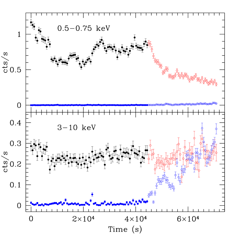
Figure 3: The top panel shows the background subtracted source (black and red) and background (blue) light curve in the 0.5–0.75 keV band, respectively. The bottom panel plots the background subtracted source light curve (black and red) and background light curve (blue) in the 3–10 keV band, respectively. The bin size is 600 s and the time zero is JD=2454368.21282. The background light curves clearly show that the high background, starting from $\sim 45$ ks to the end of the observation, is mostly significant in the high energy band. The open symbols indicate the high background interval.

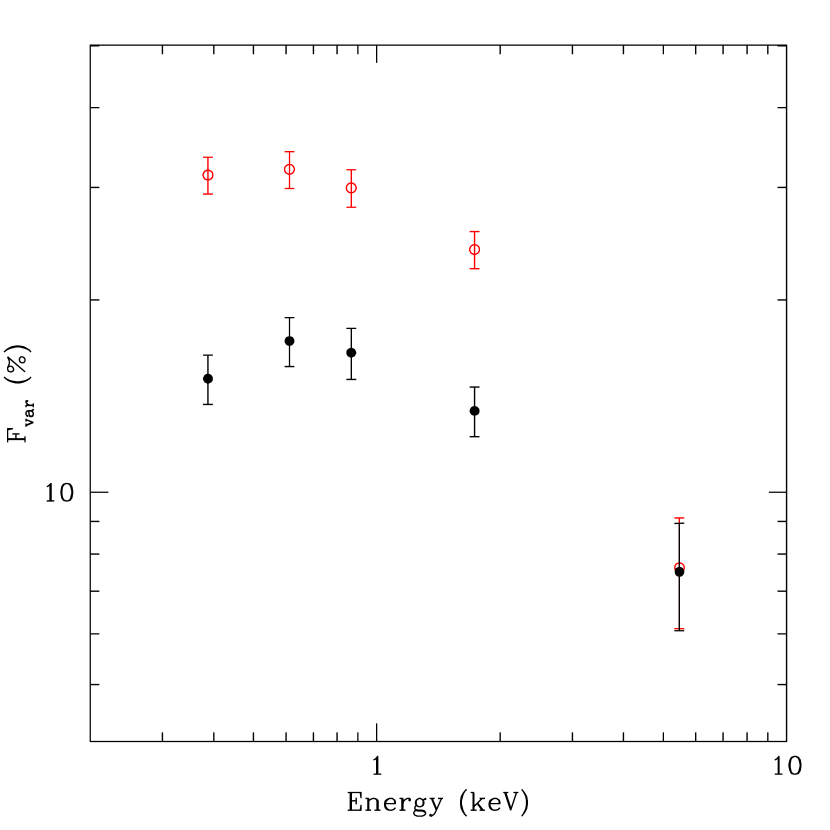
Figure 4: The variability amplitude ($F_{\rm var}$) as a function of photon energy. The black solid symbols are calculated by excluding the high background interval, while the red open symbols are calculated with the entire observation.

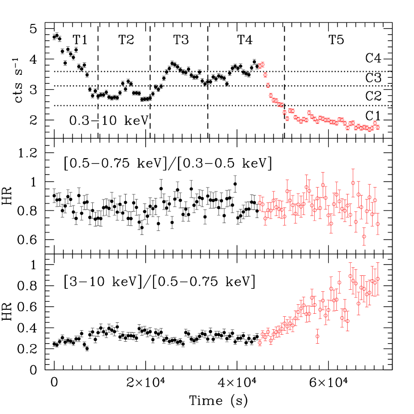
Figure 5: From top to bottom panels are shown the background subtracted 0.3–10 keV light curve, and the temporal evolution of the 0.5–0.75 to 0.3–0.5 keV hardness ratios and of the 3–10 to 0.5–0.75 keV hardness ratios, respectively. The top panel also shows the time intervals (the vertically dashed lines) used for the time resolved spectral analysis, and the count rate intervals (the horizontally dotted lines) used for the count rate resolved spectral analysis (see Section 3.3). The data have a binsize of 600 s. The red open circles show the time interval affected by the high background.

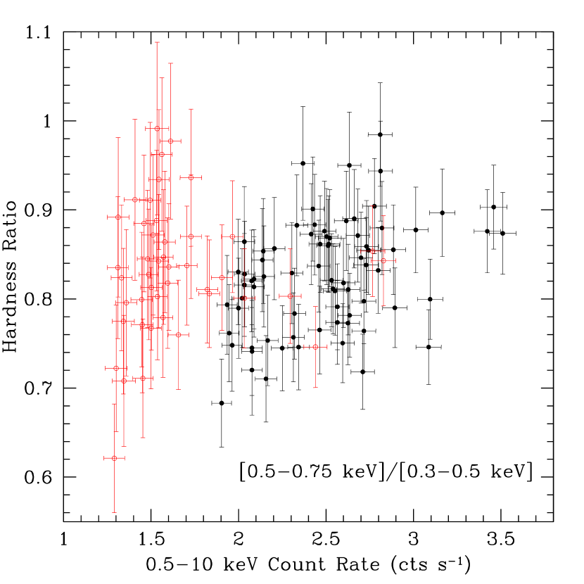
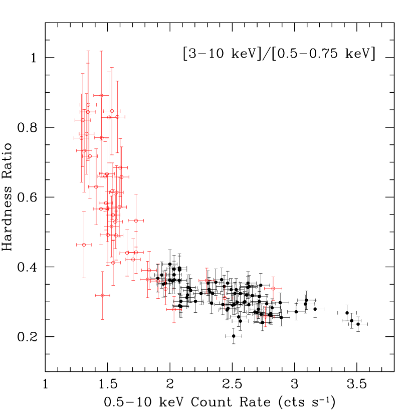
Figure 6: Relationship between the hardness ratios and the count rates. Left plot is for the 0.5–0.75 to 0.3–0.5 keV hardness ratios versus the 0.5–10 keV count rates. Right plot is for the 3–10 to 0.5–0.75 keV hardness ratios versus the 0.5–10 keV count rates. The data have a time binszie of 600 s. The red open circles indicate the data polluted by the high background.

Figure 3 shows the 600 s binned background subtracted light curve in the 0.5–0.75 and 3–10 keV band, respectively. The corresponding background light curves are also plotted for comparisons, clearly showing that the background is significantly high from the $\sim 45$ ks to the end of the observation. The background, however, is high in the hard X-ray band only. In order to study the entire observation, we discriminate the time interval affected by the high background with open symbols in Figures 3–6.

The 0.5–0.75 keV light curve illustrates that the source is strongly variable in the soft X-ray band. The variability of a factor of $\sim 4$ is quantified by the ratio of the maximum to minimum count rates over the whole observation. The light curve is plenty of characteristics. It initially decreases by a factor of $\sim 2$ over a timescale of $\sim 8$ ks (i.e., the halving timescale is $\sim 8$ ks), followed by a small amplitude flare with duration of $\sim 6$ ks. Afterwards, a large amplitude flare occurs. The count rates increase by a factor of $\sim 1.5$ on a timescale of $\sim 7$ ks. Then another flare of similar amplitude appears to happen, whose rising phase may overlap with the decaying phase of its anterior flare. Starting from the $\sim 46$ ks of the observation, the source decreases rapidly by a factor of $\sim 2$ over a timescale of $\sim 7$ ks, followed by a slow decay till the end of the observation.

However, the 3–10 keV light curve shows only a weak trend of variability, with roughly $50\%$ changes from the minimum to maximum count rate. From the beginning to $\sim 50$ ks of the observation, the hard band light curve approximately follows the soft band light curve. Nevertheless, during the last part of the observation, the hard band light curve becomes erratic, probably caused by the high background, and does not track the soft band light curve.

Accordingly, S5 0716+714 is much more variable in the soft than in the hard X-ray band. We use the factional variability amplitude ($F_{\rm var}$, e.g., Zhang et al. 1999) to quantify the source’s variability. In the 0.5–10 keV band, $F_{\rm var}$ is ($25.2\pm 1.6$)%. In order to study the energy dependence of the variability amplitude, we calculate $F_{\rm var}$ in five (0.3–0.5, 0.5–0.75, 0.75–1, 1–3 and 3–10 keV) energy bands. The results are tabulated in Table 4. In Figure 4, $F_{\rm var}$ is plotted against the photon energy, where the solid and open symbols indicate the results by excluding and including the high background interval, respectively. Except for the different values of $F_{\rm var}$, the energy dependence of $F_{\rm var}$ is similar for the two scenarios. $F_{\rm var}$ increases from the 0.3–0.5 keV to the 0.5–0.75 keV, then it decreases with higher energies.

In Figure 5, we plot, from the top to bottom panels, the 0.3–10 keV light curve, and the temporal evolution of the 0.5–0.75 to 0.3–0.5 keV hardness ratios (representing the soft X-ray spectra) and the 3–10 to 0.5–0.75 keV hardness ratios (representing the overall X-ray spectra), respectively. The 0.5–0.75 to 0.3–0.5 keV ratios appear to follow the light curve, in the sense that the soft X-ray spectra flatten with increasing fluxes. On the contrary, the 3–10 to 0.5–0.75 keV ratios seem to anti-correlate with the light curve, indicating that the overall spectra soften with increasing fluxes.

The left plot of Figure 6 shows the relationship between the 0.5–0.75 to 0.3–0.5 keV ratios and the 0.5–10 keV count rates. Except for the data contaminated by the high background, the hardness ratios appear to increase with higher count rates, showing the harder-when-brighter trend for the soft X-ray variations. The right plot of Figure 6 presents the relationship between the 3–10 to 0.5–0.75 keV ratios and the 0.5–10 keV count rates. It is clear that the hardness ratios become smaller with higher count rates, indicating the softer-when-brighter phenomenon for the overall X-ray variations.

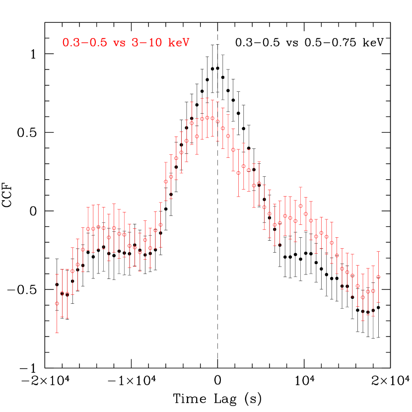
Figure 7: The black solid circles show the CCF between the 0.3–0.5 and 0.5–0.75 keV light curve, peaking at zero lag. The red open circles present the CCF between the 0.3–0.5 and 3–10 keV light curve, peaking at $-1200$ s. The negative lags indicate a delay of the lower energy with respect to the higher energy light curve. The light curves and the CCFs are binned over 600 s. The high background interval is excluded when calculating the CCFs.

Due to the long orbital period, XMM-Newton is able to produce continuously sampled light curves over about one day, which is very important to study the inter-band time lags of the intra-day X-ray variability of blazars. The lags can thus be estimated by calculating the standard Cross-Correlation Function (CCF) between any two energy band light curves. We calculate the CCFs between the 0.3–0.5 keV and the higher energy light curves. The time interval affected by the high background are excluded. Figure 7 plots the CCFs of the 0.3–0.5 keV with respect to the 0.5–0.75 and 3–10 keV band, respectively. A negative lag indicates that the lower energy variations lag the higher energy ones (i.e., soft lag). The CCF of the 0.3–0.5 keV versus the 0.5–0.75 keV peaks at zero lag, but the slight asymmetry towards negative lags suggests a possible soft lag of $<600$ s. However, the CCF between the 0.3–0.5 and 3–10 keV peaks at the lag of $-1200$ s, suggesting a soft lag of $\sim 1200$ s. We estimate the lags with three techniques: (1) $\tau_{\rm peak}$ is the lag corresponding to the CCF peak ($\rm CCF_{\rm max}$); (2) $\tau_{\rm cent}$ is obtained by computing the CCF centroid; and (3) $\tau_{\rm fit}$ is the lag corresponding to the peak of a Gaussian function (plus a constant) fitted to the CCF. Both $\tau_{\rm cent}$ and $\tau_{\rm fit}$ are measured within the CCF lag range of $[-7000,7000]$ s only. The results are tabulated in Table 4, where the uncertainties on $\tau_{\rm fit}$ are $1\sigma$ confidence level. Although $\tau_{\rm peak}$ is zero for the CCFs of the 0.3–0.5 keV with respective to the 0.5–0.75, 0.75–1 and 1–3 keV, the estimated values of $\tau_{\rm cent}$ and $\tau_{\rm fit}$ suggest soft lags of $\sim 200-600$ s, smaller than the binsize (600 s) of the light curves. This means that for the three cases, the CCFs may peak at lags of 0–600 s rather than at zero if the light curves were binned with smaller binsizes (e.g., 100 s). Interestingly, from the point view of $\tau_{\rm cent}$ or $\tau_{\rm fit}$, the soft lags become larger with larger energy differences.

3.3 Spectral Variability

In order to investigate the spectral variability of the synchrotron and IC emission and their sum, respectively, we divide the entire observation into several intervals in two ways. The first division is by time order. We identify the 0.3–10 keV light curve as five ”isolated” episodes, separated with the vertically dashed lines in the top panel of Figure 5 and numbered as T1, T2, T3, T4 and T5 in time order. T1 may represent a decay phase (possibly part) of a large amplitude flare. T2 covers mainly a low amplitude flare. T3 and T4 present two pronounced flares. The decaying phase of T3 and the rising phase of T4 may overlap with each other. T4 is complicated, consisting of a couple of small amplitude flares. T5 is a long slow decay. Then we divide the observation on the basis of the 0.5–10 keV count rates. We choose four count rate intervals, differentiated with the horizontally dotted lines in the top panel of Figure 5 and numbered as C1, C2, C3 and C4 from the low to high count rates. C4 is the highest state, covering the peaks of T1, T3 and T4. We mention that C1 is roughly identical to T5, as the quiescent state in both divisions. Since they are affected by the high background, we separate the T5 and C1 intervals from other intervals. The T5 and C1 spectra might be distorted by the high background.

We repeat spectral fits for each time and count rate interval with the broken and double power law plus the Galactic absorption. The broken power law presents a visual inspection of the break energy from the synchrotron to IC dominance. The double power law determines the crossing energy, at which the fluxes of the two emission components are equal. Our main purpose is to study the changes of the break and crossing energies with the source’s intensities. The results of the spectral fits are summarized in Table 5 and Table 6 for the broken and double power law, respectively, showing that all fits are acceptable. In most cases, however, the fits are somewhat better for the double power law than for the broken power law. It is important to note that the crossing energies, depending on the photon indices and the normalization of the two components, are not identical to the break energies in general.

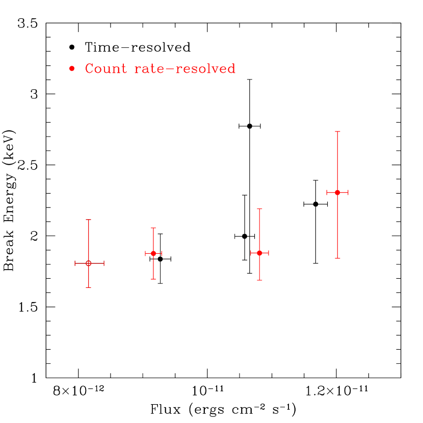
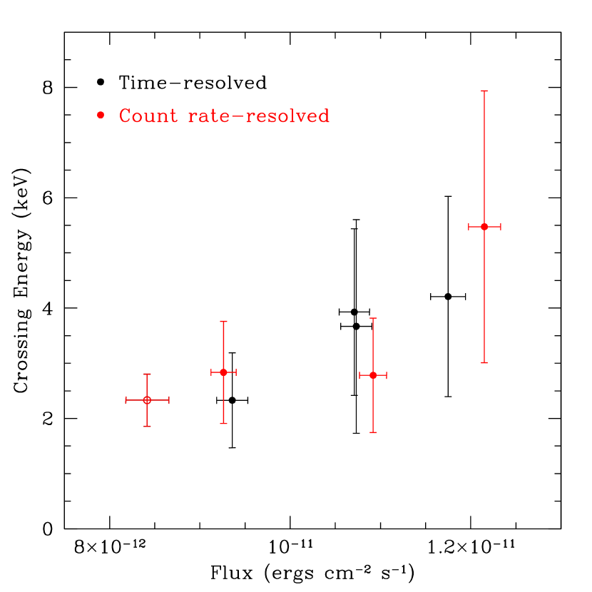
Figure 8: The left plot shows the relationship between the break energies and the 0.5–10 keV total fluxes, derived from the broken power law fit. The right plot shows the relationship between the crossing energies (of the synchrotron and IC components) and the 0.5–10 keV total fluxes, derived from the double power law fit. The black symbols are for the time-resolved intervals, and the red symbols for the count rate-resolved intervals. The open symbol indicates the T5/C1 interval together, which is affected by the high background.

Figure 8 plots the break and crossing energies as a function of the 0.5–10 keV total fluxes. The two kinds of energies increase when the fluxes increase, but the crossing energies appear to increase more rapidly with the fluxes than the break energies does.

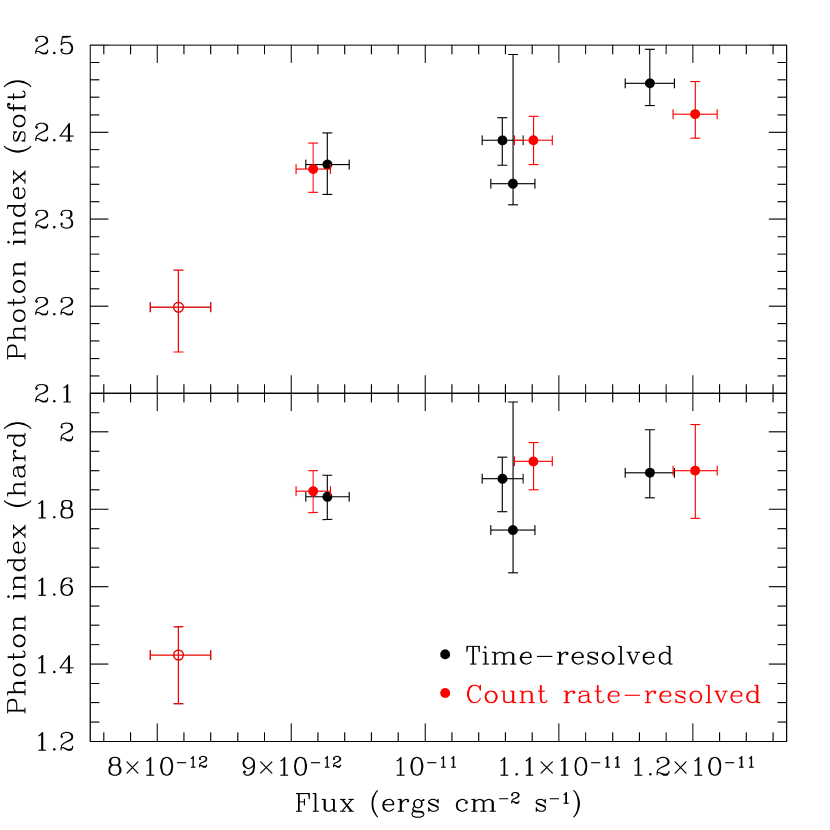
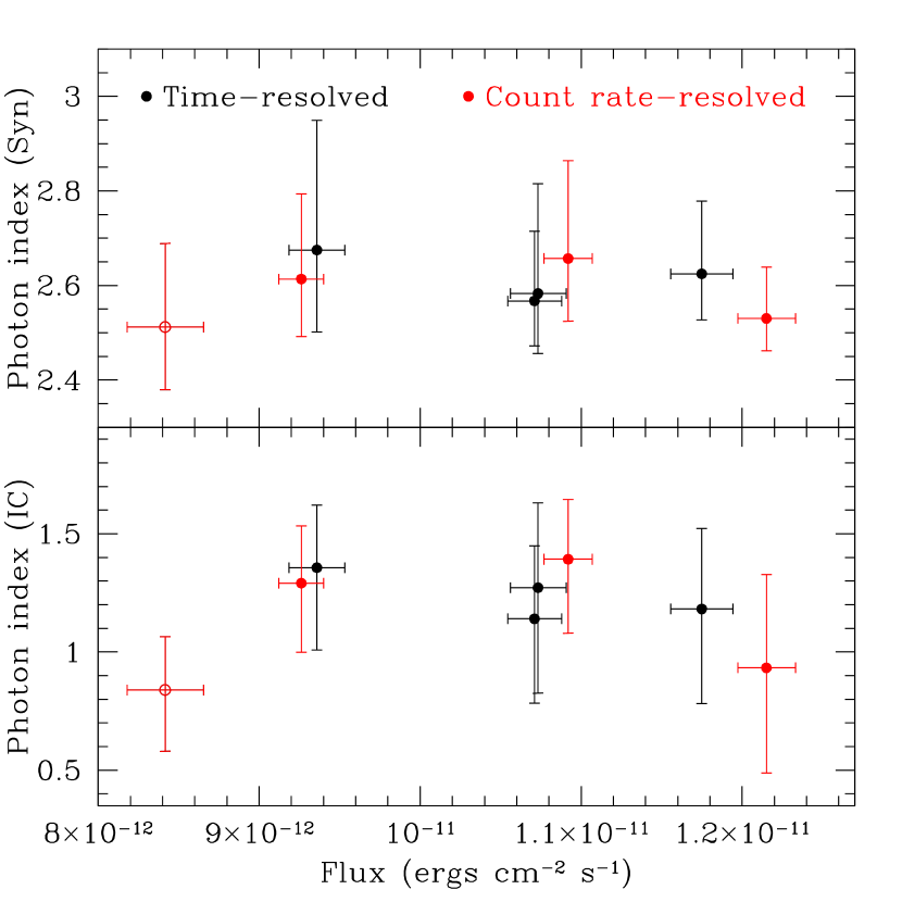
Figure 9: The photon indices are plotted against the 0.5–10 keV total fluxes. The left plot shows the soft and hard X-ray photon indices, derived from the broken power law fit. The right plot shows the synchrotron (Syn) and IC photon indices, derived from the double power law fit. The black symbols are for the time-resolved intervals, and the red symbols for the count rate-resolved intervals. The open symbol indicates the T5/C1 interval together, which is affected by the high background.

In Figure 9, we show the relationships between the photon indices and the 0.5–10 keV total fluxes. For the broken power model, there is weak correlation, showing that the soft photon indices become larger (the spectra become steeper) with increasing fluxes. However, except for the T5/C1 point, the hard photon indices are roughly identical within the uncertainties. It is worth noting that the break energies change by $\sim 0.5$ keV between different intervals, indicating that the soft and hard photon indices are actually measured in different energy ranges. Therefore, the implications for the changes of the soft and hard photon indices are somewhat vague. For the double power law model, the synchrotron and IC photon indices do not correlate with the fluxes. In fact, they are consistent with each other within the error bars, no matter the synchrotron or IC photon indices.

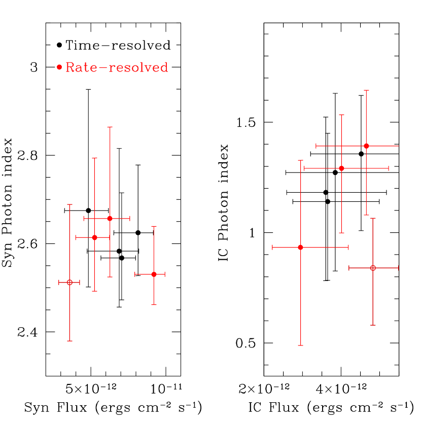
Figure 10: The left panel plots the relationship between the synchrotron (Syn) photon indices and the 0.5–10 keV synchrotron fluxes. The right panel plots the relationship between the IC photon indices and the 0.5–10 keV IC fluxes. The black symbols are for the time-resolved intervals, and the red symbols for the count rate-resolved intervals. The open symbol indicates the T5/C1 interval together, which is affected by the high background. Besides the T5/C1 whose spectrum might be affected by the high background, the synchrotron spectra appear to harden with higher synchrotron fluxes, while the IC spectra appear to soften with higher IC fluxes.

The left panel of Figure 10 plots the relationship between the synchrotron photon indices and the 0.5–10 keV synchrotron fluxes. Although they might be identical within the uncertainties, the synchrotron photon indices appear to become smaller (i.e., the synchrotron spectra harden) with higher synchrotron fluxes. The right panel of Figure 10 shows the relationship between the IC photon indices and the 0.5–10 keV IC fluxes. Although their uncertainties are large, the IC photon indices exhibit larger changes with respect to the synchrotron ones. Contrary to the synchrotron spectral behaviour, the IC photon indices appear to become larger (i.e., the IC spectra soften) with larger IC fluxes.

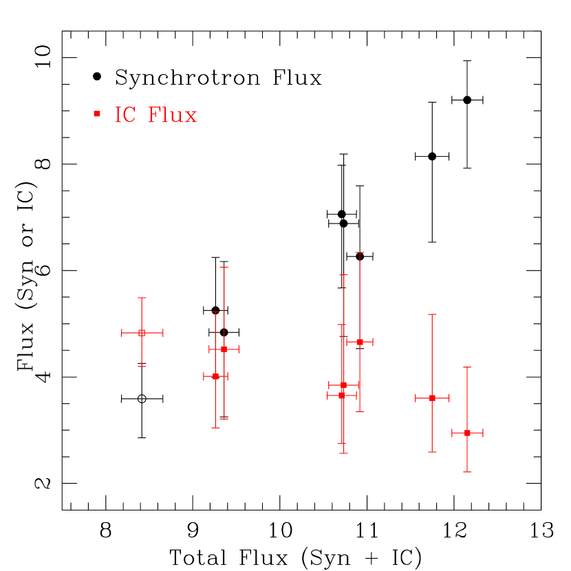
Figure 11: The synchrotron (Syn) and IC 0.5–10 keV fluxes are plotted against the total (synchrotron plus IC) 0.5–10 keV fluxes. The fluxes are in unit of $\rm{10^{-12}~{}ergs~{}cm^{-2}~{}s^{-1}}$. The open symbol indicates the T5/C1 interval together, which is affected by the high background.

In Figure 11, the synchrotron and IC 0.5–10 keV fluxes are plotted against the total (synchrotron plus IC) 0.5–10 keV fluxes, respectively. With increasing total fluxes, the synchrotron fluxes increase but the IC fluxes decrease, indicating that the synchrotron fluxes anti-correlate with the IC fluxes. Figure 11 also shows that the synchrotron fluxes have larger changes than the IC fluxes. Similar relationships can be obtained if the synchrotron and IC 0.5–2 keV (or 2–10 keV) fluxes are plotted against the total 0.5–10 keV (or 0.5–2 keV, 2–10 keV) fluxes, respectively.

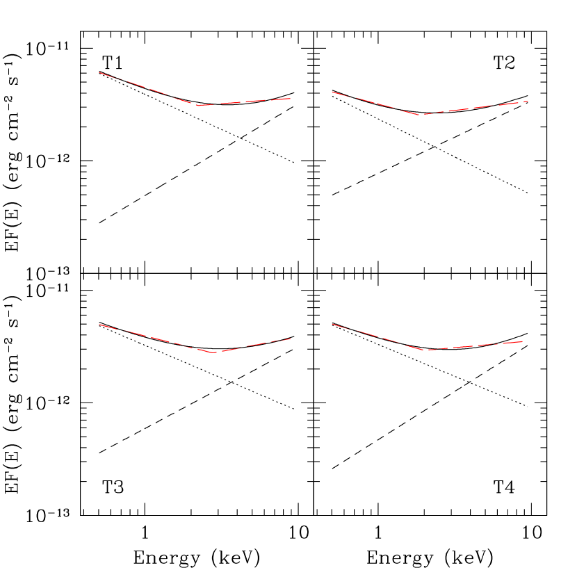
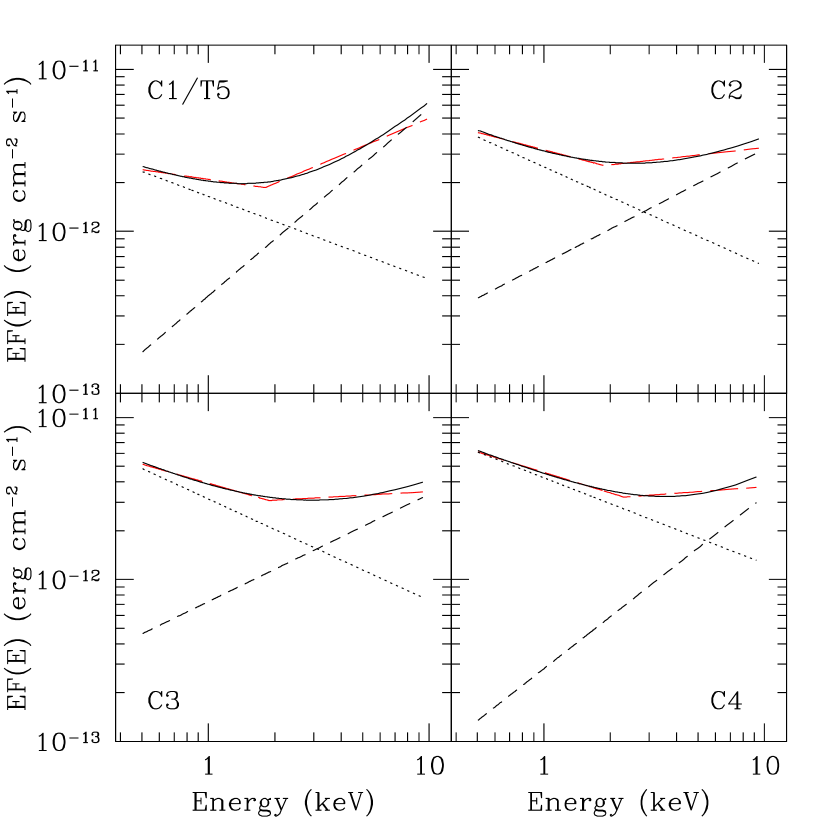
Figure 12: The evolution of the unabsorbed X-ray SEDs. The black dotted, short dashed and solid lines show the synchrotron and IC component and the sum of the two, respectively, unfolded with the double power law. The red long dashed line shows the SEDs unfolded with the broken power law. The T5 and C1 interval are identical, shown as one, which are affected by the high background.

The evolutions of the unabsorbed 0.5–10 keV X-ray SEDs are shown in Figure 12. We plot the SEDs unfolded with the double and broken power laws together to show their differences. The SED differences between the two models are visible, as viewed by the disagreements between the SED break energies (the broken power law) and the SED trough energies (the double power law). Their SEDs also show clear differences in the highest energy band.

In Figure 12, the synchrotron and IC SEDs are also plotted to show the evolutions of the two components separately and their crossing energies. The crossing energies are obviously larger than the break energies. The SED (double power law) trough energies are smaller than the crossing energies in most cases. When the source brightens, the synchrotron emission extends to higher energies, whereas the IC emission recedes from lower energies. Moreover, with higher total fluxes, the synchrotron fluxes have larger increases than the IC fluxes. At the same same, the synchrotron spectra harden with higher synchrotron fluxes, while the IC spectra soften with larger IC fluxes (see also Figure 10). Therefore, the crossing energies become larger when the source brightens (see also the right plot of Figure 8). It is important to note that the extensions of the synchrotron component to higher energies are mainly caused by the significant increases of its normalization rather than by its spectral hardening. The changes of the synchrotron spectral slopes are in fact small. The normalization changes of the IC component are small, while the changes of its slopes are relatively large.

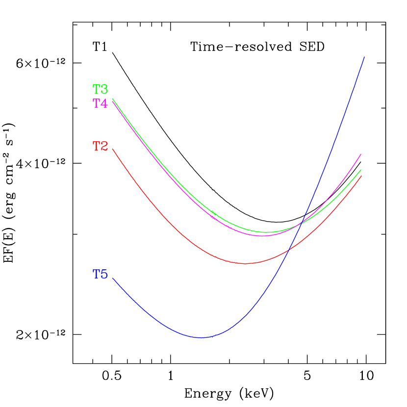
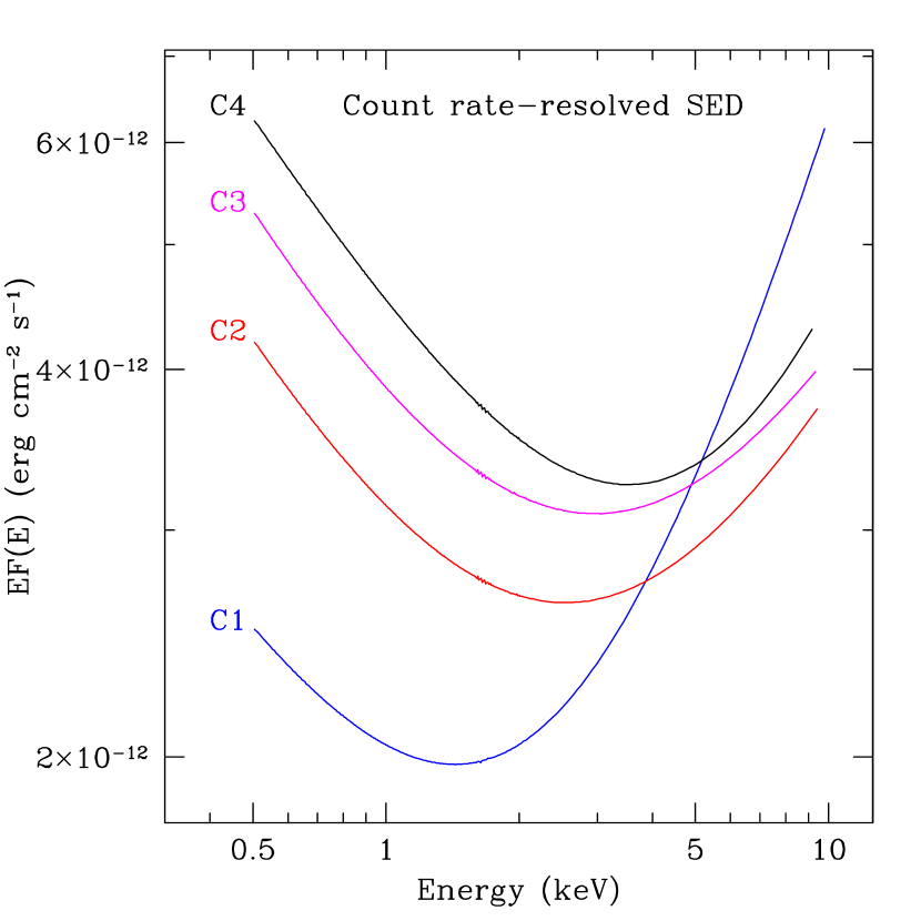
Figure 13: The evolution of the unabsorbed X-ray SEDs (the sum of the synchrotron and IC component) unfolded with the double power law. With increasing total fluxes, the synchrotron emission extends to higher energies, while the IC emission recedes from lower energies. The T5 and C1 interval are identical, which are affected by the high background.

Figure 13 clearly shows the evolution of the 0.5–10 keV X-ray SEDs unfolded with the double power law. Except for the T5 and C1 SEDs, the SED slopes below the trough energies appear to not change significantly with the fluxes, whereas the SED slopes above the trough energies show larger changes with the fluxes. Due to small changes of the IC fluxes, the shift of the SED troughs to higher energies with increasing fluxes is primarily caused by the increases of the synchrotron fluxes. The significant hardening of the T5 and C1 SEDs above the trough energies might be affected by the high background, since their SED slopes below the trough energies are similar to those of other intervals.

4 OM data analysis

The OM observation provides optical/UV data simultaneous to the X-ray observation. The data at each filter provide a time coverage of $\sim 15$ ks, showing short-term variability of S5 0716+714 in the optical-UV wavelengths.

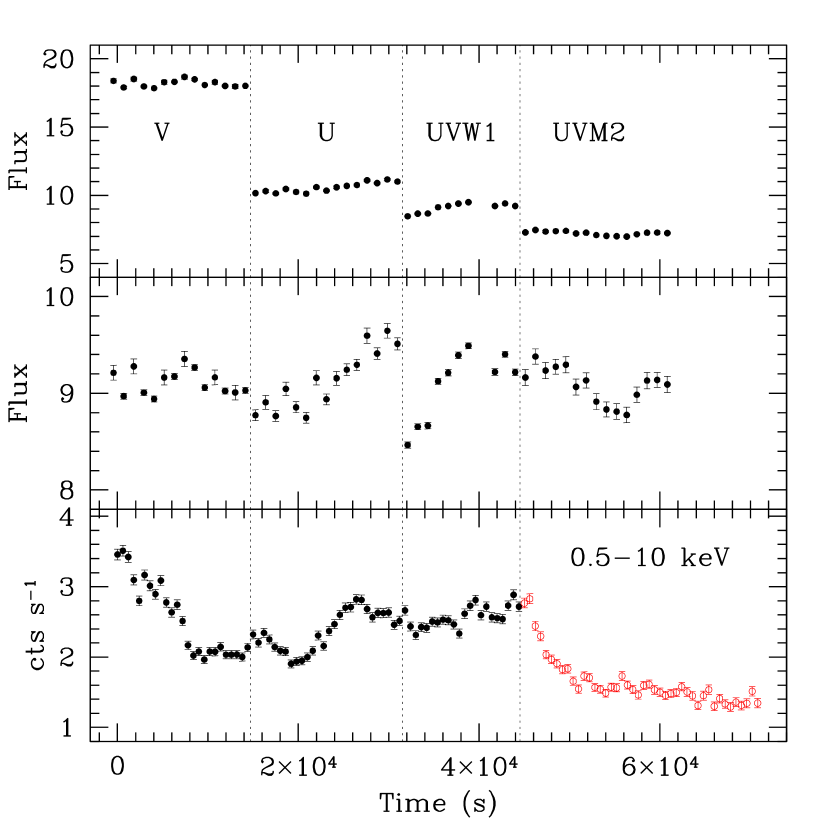
Figure 14: The upper panel plots the light curves in different OM filters (the error bars on fluxes are smaller than the symbol sizes). The middle panel shows the scaled UVW1 band light curve. The fluxes are in unit of $10^{-26}~{}{\rm ergs}~{}{\rm cm}^{-2}~{}{\rm s}^{-1}~{}{\rm Hz}^{-1}$. The bottom panel presents the 0.5–10 keV light curve. The vertical dotted lines separate the time intervals covered by different OM filters, allowing an easy comparison between the light curves of different OM filters and the X-ray light curve over the same time range.

The count rates are converted into fluxes using the conversion factors for a white dwarf, as recommended by the OM calibration manual. Using the extinction curve of Cardelli et al. (1989) and the extinction parameters of $R_{V}=3.1$ and $A_{V}=0.102$, we correct the fluxes with the extinction coefficient at the effective wavelength of each filter. The value of $A_{V}$ is taken from NED, which was obtained by following Appendix B of Schlegel et al. (1998). The OM light curves after extinction correction are shown in the top panel of Figure 14 with filter name indicated.

The fluxes gathered with different filters can not be used to do a straightforward comparison with the X-ray light curve for the whole observational length. We thus scale all the V, U and UVM2 fluxes to the fluxes at the effective wavelength of the UVW1 filter ($\lambda=291$ nm). We assume a power law spectrum between any pair of filters, whose spectral index is calculated with the average fluxes at the two filters. The scaled UVW1 light curve is shown in the middle panel of Figure 14. By adopting a constant spectral index to scale the fluxes from one filter to UVW1, the scaled UVW1 light curve keep the same shape as the original one. For each filter, our scaling law changes its flux level only. The 0.5–10 keV light curve is also shown in the bottom panel of Figure 14 for a visual comparison with the scaled UVW1 light curve. It is important to emphasize that the scaled UVW1 light curve is just used to make a general comparison rather than to build strict correlation with the X-ray light curve, since the scaled UVW1 fluxes might be sufficiently different from the true UVW1 fluxes due to the known spectral variability of the source in the optical-UV range.

The scaled UVW1 light curve does not closely track the X-ray one throughout the observation. The most significant difference might be the sharp transition from the last U-to-UVW1 scaled flux to the first UVW1 flux, which does not have a correspondence in the X-ray light curve. Nevertheless, it is certain that the variability amplitude is significantly smaller in the UVW1 band than in the X-ray band.

It is also possible to compare the OM light curves in different filters with the X-ray light curve over the same time intervals, respectively. It is clear that the V, UVW1 and UVM2 light curves do not follow the X-ray light curve. The decay of $\sim 8$ ks long in the X-ray light curve is not seen in the V band light curve. Instead, the V light curve seems to show a well-defined micro-flare. The UVW1 light curve displays a rise of $\sim 6$ ks long, which is not clear in the corresponding X-ray light curve. The UVM2 light curve shows a decay followed by a rise, whereas the X-ray light curve exhibits a rapid decay followed by a slow decay. However, the U light curve appears to track the X-ray light curve, where the peaks in the U light curve show a delay of $\sim 2$ ks with respect to the ones in the X-ray light curve.

The OM data also extend the synchrotron SED of the source to the optical-UV range, where the synchrotron emission may peak around. Figure 15 plots the average optical-UV-X-ray SED. The four optical-UV data points appear to be roughly on the extrapolation of the soft X-ray SED, suggesting the same origin of the optical-UV and soft X-ray emission.

5 Discussion and Conclusions

We perform a detailed spectral and temporal analysis for the second XMM-Newton observation of S5 0716+714. Most of our results are in agreement with previous results obtained from the first XMM-Newton observation (FE06) and other X-ray observations (e.g., Giommi et al. 1999; Tagliaferri et al. 2003). Nevertheless, we also find some new phenomena, adding new clues to better understand the underlying physical processes taking place in the source.

The concave X-ray spectra of S5 0716+714 can be disentangled into two power law components. The steep power law ($\Gamma\sim 2.6$) component is interpreted as the high energy tail of the synchrotron emission, whereas the flat power law ($\Gamma\sim 1.2$) component is ascribed to the low energy side of the IC emission. FE06 obtained similar results with the first XMM-Newton observation. It is worth noting that the photon indices of the steep power law component are similar to those of HBLs in the hard X-ray band (e.g., PKS 2155–304: Zhang 2008), supporting the interpretation of the steep power law component as the synchrotron tail.

The X-ray variability amplitude of HBLs monotonically increases with higher energy (e.g., PKS 2155–304: Zhang et al. 2005; Mrk 421: Zhang et al. 2010), which is thought to be the signature of synchrotron emission. However, LBLs are highly variable in the soft X-rays, whereas they show little variability in the hard X-rays (e.g., Giommi et al. 1999). Our results demonstrate that S5 0716+714 is indeed strongly variable in the soft X-rays, showing the maximum variability by a factor of $\sim 4$ throughout the whole observation and several episodes of rapid variations on timescales of hours. In a sharp-cut contrast, the hard X-ray fluxes of the source are much less variable, exhibiting only $\sim 50\%$ change between the minimum and maximum count rates and no rapid events. For the first time, we quantify the energy dependence of the variability amplitude for S5 0716+714. The variability amplitude increases from the 0.3–0.5 to 0.5–7.5 keV band, but from the 0.75–1 keV band, it decreases with higher energy. Moreover, the OM data suggest lower variability amplitude in the UV band than in the soft X-ray band. The energy dependence of the variability amplitude of S5 0716+714 is thus clearly different from those of HBLs.

During the first XMM-Newton observation, the $F_{\rm var}$ of S5 0716+714 amounts to $40\pm 3\%$ in the 0.5–0.75 keV and $27\pm 1\%$ in the 3–10 keV (FE06). Though longer duration of the second XMM-Newton observation, the $F_{\rm var}$ is only $32.03\pm 2.12\%$ and $7.62\pm 1.5\%$ in the corresponding energy bands. It is important to understand whether the synchrotron or IC emissions or both are responsible for the significant variations of S5 0716+714 in different energy bands. It is usually argued that the variable high energy tail of the synchrotron emission is responsible for the highly variable soft X-ray emission, whereas the ”stable” low energy side of the IC emission accounts for the lack of variability in the hard X-ray band (e.g., Giommi et al. 1999; Tagliaferri et al. 2003). This argument is somewhat ambiguous, since the two XMM-Newton observations clearly demonstrate that the hard X-ray fluxes are also highly variable, although their variability amplitudes are significantly smaller than the soft X-ray ones. The hard X-ray variations could be due to either the IC or synchrotron variations. It is certain that the synchrotron component is strongly variable on short timescales, whereas it is unclear whether the IC component is variable on similar timescales. The spectral analysis by FE06 showed that the IC component might be variable on timescales of hours, which is, however, not supported by our results. Although the IC component contributes more to the total hard X-ray fluxes, we still assume that the hard X-ray variations might be controlled by the synchrotron tail. With increasing energies, the increasing dilutions of the ”stable” IC component to the increasing variations of the synchrotron tail, might result in the observed overturn of the energy-dependent variability amplitude for S5 0716+714.

The model-independent hardness-ratio analysis shows that the 0.5–10 keV spectra of S5 0716+714 soften when it brightens. The phenomenon, also noticeable in the first XMM-Newton observation (FE06; Foschini et al. 2006), was already found in the BeppoSAX observations of the source (Giommi et al. 1999). The softer-when-brighter phenomenon is interpreted in terms of the high energy tail of the synchrotron emission extending more to higher energies when the source brightens (e.g., Giommi et al. 1999). Nevertheless, the soft X-ray spectra appear to harden when it brightens, though the trend is not significant. The variability property found in the soft X-ray band of the source with ROSAT observations (Cappi et al. 1994) is similar to what we found here. The harder-when-brighter trend is analogous to those of HBLs, presenting a strong evidence that the soft X-ray emission of S5 0716+714 is dominated by the synchrotron tail.

Although the inter-band time lags and the related energy dependence have been detected in a few X-ray bright HBLs, they have not be firmly detected in LBLs yet. FE06 claimed that the lags of $\gtrsim 100$ s were not present in the first XMM-Newton observation of S5 0716+714. However, we found that the 0.3–0.5 keV variations lag the 3–10 keV ones by $\sim 1000$ s in the second XMM-Newton observation. We also found a weak evidence that the lags increase with larger energy differences. In at least one episode of the optical-UV light curves, the U band variations might lag the X-ray variations by $\sim 2000$ s. As far as we know, it is the first evidence for a definite detection of soft lag in the X-ray variability of S5 0716+714 and possibly LBLs. Interestingly, the soft lags and the related energy dependence of S5 0716+714 are similar to what have been detected in HBLs (e.g., Kataoka et al. 2000; Zhang et al. 2010). The similarity suggests that the X-ray variations of the source have the same origin as those of HBLs, i.e., the variations of the synchrotron tail. Therefore, the hard X-ray fluxes of the source are dominated by the IC component, but the hard X-ray variations might be still controlled by the synchrotron tail, as already suggested by the energy dependent variability amplitude. If we assume that both the soft and hard X-ray variations are caused by the synchrotron tail, the observed soft lags provide a way to constrain the physical parameters of the emitting region (e.g., Zhang et al. 2002),

$$B\delta^{1/3}=209.91\times\left(\frac{1+z}{E_{\rm l}}\right)^{1/3}\left[\frac{1-(E_{\rm l}/E_{\rm h})^{1/2}}{\tau_{\rm soft}}\right]^{2/3}\quad{\rm G}\,,$$ (1)

where $\tau_{\rm soft}$ is the observed soft lag (in second) between the low ($E_{\rm l}$) and high ($E_{\rm h}$) energy (in keV), $z$ the source’s redshift, $B$ the magnetic field (in G) and $\delta$ the bulk Doppler factor of the emitting region. If adopting $\tau_{\rm soft}\sim 1000$ s between the 0.3–0.5 and 3–10 keV, one gets $B\delta^{1/3}\sim 2.56$ G. During a model fit to the SED involving the first XMM-Newton observation of S5 0716+714, Foschini et al. (2006) assumed $B=3$ G and $\delta=16.7$, i.e., $B\delta^{1/3}=7.67$ G. A larger $B\delta^{1/3}$ implies a smaller $\tau_{\rm soft}$, qualitatively consistent with the soft lags of no larger than 100 s claimed by FE06.

The unprecedented high signal-to-noise ratio PN observation allows us to disentangle the synchrotron and IC components in the X-ray band of S5 0716+714 and to synchronously study the variations of the two components on timescales of hours. The results, obtained with the divisions of the observation by individual episodes and by count rate levels, are consistent with each other. The synchrotron photon indices are constrained in a limited range of $\Gamma\sim 2.5-2.7$, which are typical of HBLs in the hard X-rays (e.g., PKS 2155–304: Zhang 2008). The IC photon indices show relatively large changes ($\Gamma\sim 0.9-1.4$). Due to large uncertainties, the synchrotron photon indices might be consistent with each other within the error bars, which could be also true for the IC photon indices. Although the synchrotron and IC photon indices do not correlate with the total fluxes, the synchrotron spectra appear to harden with higher synchrotron fluxes, and the IC spectra seem to soften with higher IC fluxes. When the source brightens, the synchrotron fluxes increase, while the IC fluxes decrease. The synchrotron fluxes also show larger variations than the IC fluxes.

The X-ray SEDs convolved with the synchrotron and IC components exhibit significant concave shapes. The crossing energies and the SED trough energies increase with the increasing total fluxes. The flux dependence of the crossing energies and the SED trough energies is consistent with that of the first XMM-Newton observation (FE06). We further notice that the SED trough energies are smaller than the crossing energies in most cases, indicating that they are not the exact energies at which the synchrotron component transits to the IC component in terms of the equal contributions of the two components to the total fluxes. The SED evolution, characterized by the shifts of the SED troughs to higher energies with higher fluxes, might be mainly caused by the changes of the synchrotron normalization. The changes of the synchrotron and IC photon indices and of the IC normalization may affect the SED evolution in a weaker way.

The spectral and temporal behaviors of S5 0716+714 and its synchrotron and IC emission are just the consequence of the peaks of both the synchrotron and IC SEDs shifting to higher energies with increasing fluxes. When the source brightens, the synchrotron peak moves to higher energy. In turn, the high energy tail of the synchrotron emission extends to higher energy. The synchrotron peak is therefore more close to the observed X-ray band, bring on that the synchrotron flux increases and the synchrotron spectrum hardens. At the same time, the IC peak also shifts to higher energy, incurring that the low energy end of the IC emission recedes from lower energy to the observed X-ray band. The IC peak is thus more far from the observed X-ray band. As a result, the IC flux decreases and the IC spectrum hardens. Accordingly, the synchrotron flux anti-correlates with the IC flux when the source brightens. The series of changes make the SED trough move to higher energy with higher total flux. The high energy tail of the synchrotron emission originates from the high energy electrons, showing strong and rapid variations. The low energy end of the IC emission comes from the low energy electrons, exhibiting small and slow variations. Soft lag is expected if both the soft and hard X-ray variations are caused by the cooling of the high energy electrons.

In conclusions, S5 0716+714 exhibits different X-ray variability properties between the two XMM-Newton observations. During the second observation, it shows harder synchrotron and IC spectra and lower variability amplitude. Even though the low energy end of the IC emission contributes more to the hard X-ray fluxes than the high energy tail of the synchrotron emission does, the energy dependence of the variability amplitude suggests that the hard X-ray variations might be dominated by the synchrotron tail. The large hard X-ray variability amplitude suggests its synchrotron origin as well. More importantly, soft lags are detected for the first time, also supporting that the soft and hard X-ray variations are caused by the same mechanism. When the the source brightens, the synchrotron fluxes increase but the IC fluxes decrease. The synchrotron spectra might harden with higher synchrotron fluxes, while the IC spectra might soften with larger IC fluxes. The synchrotron tail shows larger flux variations but smaller spectral variations than the IC emission does. With higher fluxes, the crossing points between the two components and the SED troughs move to higher energies. The X-ray variability of S5 0716+714 is in accordance with the results of its synchrotron and IC SED peaks shifting to higher energies with higher fluxes. The decompositions of its X-ray emission into the synchrotron and IC components are helpful to understand the behaviours of both the low and high energy part of the electron population.

Table 1: Details of the XMM-Newton EPIC-PN observation for S5 0716+714

		Date	Time				Duration	On Time	Live Time
ObsID	Orbit	(UT)	(UT)	Detector	Mode	Filter	(s)	(s)	(s)	Count Rate
0502271401	1427	2007 Sep 24	17:00:24–12:54:08	PN	SW	Thin	73917	71564	50125	2.17

Table 2: Results of XMM-Newton OM observation (Imaging Mode)

Filter	Wavelength (nm)	Date (UT)	Exp. time (s)	Exp. number	Count Rate	Magnitude	Flux
V	543	16:51:25–21:07:47	800	14	$67.03\pm 0.10$	$13.39\pm 0.01$	$1.836\pm 0.003$
U	344	21:13:08–01:48:11	800	15	$117.52\pm 0.19$	$13.08\pm 0.01$	$2.652\pm 0.004$
UVW1	291	01:53:31–05:25:07	800	10	$56.44\pm 0.06$	$12.83\pm 0.01$	$3.202\pm 0.003$
UVM2	231	05:30:28–10:05:30	800	15	$14.09\pm 0.03$	$12.90\pm 0.01$	$4.042\pm 0.009$

Table 3: Results of X-ray spectral fits to the average X-ray spectrum

		$E_{\rm break}$(keV)/	$\Gamma_{2}$/			Flux	Flux
Model	$\Gamma_{1}$	$\beta$	$kT$(keV)	$\chi^{2}_{\nu}$/dof	Prob.	(2–10 keV)	(0.5–10 keV)
Single power law	$2.25\pm 0.01$	–	–	1.73/792	$2.7\times 10^{-33}$	$4.39\pm 0.06$	$9.85\pm 0.07$
Broken power law	$2.38\pm 0.02$	$1.94^{+0.32}_{-0.11}$	$1.92^{+0.03}_{-0.07}$	1.05/790	0.18	$5.13\pm 0.08$	$10.54\pm 0.08$
Double power law	$2.56^{+0.09}_{-0.07}$	–	$1.22^{+0.19}_{-0.21}$	1.00/790	0.53	$5.23\pm 0.08$	$10.66\pm 0.09$
Logarithmic parabola	$2.37\pm 0.01$	$-0.37\pm 0.02$	–	1.01/791	0.43	$5.19\pm 0.08$	$10.62\pm 0.09$
Power law + black body	$2.40\pm 0.02$	–	$2.24^{+0.13}_{-0.16}$	1.02/790	0.35	$5.16\pm 0.09$	$10.59\pm 0.09$
Power law + bremss.	$1.93\pm 0.03$	–	$0.38\pm 0.03$	1.04/790	0.21	$5.14\pm 0.08$	$10.55\pm 0.08$

Table 4: $F_{\rm var}$ and lags

Band (keV)	$F_{\rm var}$(%)	$\rm CCF_{\rm max}$	$\tau_{\rm peak}$(s)	$\tau_{\rm cent}$(s)	$\tau_{\rm fit}$(s)
0.3–0.5	$15.06\pm 1.33$	…	…	…	…
0.5–0.75	$17.25\pm 1.51$	0.91	0	$-379$	$-210^{+188}_{-191}$
0.75–1	$16.54\pm 1.52$	0.90	0	$-394$	$-364^{+190}_{-196}$
1–3	$13.41\pm 1.20$	0.90	0	$-554$	$-593^{+184}_{-188}$
3–10	$7.508\pm 1.43$	0.59	$-1200$	$-908$	$-1084^{+385}_{-392}$

Table 5: Results of X-ray spectral fits with the broken power law

Interval	$\Gamma_{1}$	$E_{\rm break}$	$\Gamma_{2}$	K	$\chi^{2}_{\nu}$/dof	Prob.	F${}_{2-10~{}{\rm keV}}$	F${}_{0.5-10~{}{\rm keV}}$
Time resolved interval
T1	$2.46^{+0.04}_{-0.03}$	$2.22^{+0.17}_{-0.42}$	$1.89^{+0.11}_{-0.06}$	$2.79\pm 0.03$	1.02/400	0.38	$5.39\pm 0.17$	$11.68\pm 0.18$
T2	$2.36^{+0.04}_{-0.03}$	$1.84^{+0.18}_{-0.17}$	$1.83\pm 0.06$	$1.99\pm 0.03$	1.08/398	0.12	$4.80\pm 0.15$	$9.27\pm 0.16$
T3	$2.34^{+0.15}_{-0.02}$	$2.77^{+0.33}_{-1.04}$	$1.75^{+0.33}_{-0.11}$	$2.45^{+0.02}_{-0.10}$	1.00/448	0.50	$5.16\pm 0.15$	$10.66\pm 0.17$
T4	$2.39\pm 0.03$	$2.00^{+0.29}_{-0.17}$	$1.88^{+0.06}_{-0.08}$	$2.39\pm 0.02$	1.05/517	0.22	$5.20^{+0.15}_{-0.14}$	$10.58\pm 0.15$
T5	$2.20^{+0.04}_{-0.05}$	$1.81^{+0.31}_{-0.17}$	$1.42^{+0.07}_{-0.13}$	$1.31\pm 0.02$	0.99/668	0.53	$5.24^{+0.23}_{-0.21}$	$8.16^{+0.24}_{-0.21}$
Count rate resolved interval
C1	$2.20^{+0.04}_{-0.05}$	$1.81^{+0.31}_{-0.17}$	$1.42^{+0.07}_{-0.13}$	$1.31\pm 0.02$	0.99/668	0.53	$5.24^{+0.23}_{-0.21}$	$8.16^{+0.24}_{-0.21}$
C2	$2.36\pm 0.03$	$1.88\pm 0.18$	$1.85\pm 0.05$	$1.99\pm 0.02$	1.07/535	0.11	$4.69\pm 0.12$	$9.16\pm 0.13$
C3	$2.39\pm 0.03$	$1.88^{+0.31}_{-0.19}$	$1.92^{+0.05}_{-0.07}$	$2.45\pm 0.02$	0.94/513	0.83	$5.29\pm 0.13$	$10.81\pm 0.14$
C4	$2.42^{+0.04}_{-0.03}$	$2.31^{+0.43}_{-0.46}$	$1.90\pm 0.12$	$2.86\pm 0.03$	0.95/472	0.78	$5.57\pm 0.15$	$12.02\pm 0.16$

Table 6: Results of X-ray spectral fits with the double power law

	$\Gamma_{1}$	$\Gamma_{2}$			Ecross	Flux(Syn %)	Flux(Syn %)	Flux(Syn %)
Interval	(Syn.)	(IC)	$\chi^{2}_{\nu}$/dof	Prob.	(keV)	(0.5–2 keV)	(2–10 keV)	(0.5–10 keV)
Time resolved interval
T1	$2.62^{+0.15}_{-0.10}$	$1.18^{+0.34}_{-0.40}$	1.03/400	0.31	$4.21\pm 1.81$	$6.29^{+0.07}_{-0.06}$(88.6%)	$5.46\pm 0.18$(47.1%)	$11.75\pm 0.19$(69.3%)
T2	$2.67^{+0.27}_{-0.17}$	$1.36^{+0.27}_{-0.35}$	1.07/398	0.15	$2.33\pm 0.86$	$4.50\pm 0.05$(75.4%)	$4.86\pm 0.16$(29.8%)	$9.36\pm 0.17$(51.7%)
T3	$2.58^{+0.23}_{-0.13}$	$1.27^{+0.36}_{-0.45}$	0.95/448	0.77	$3.67\pm 1.94$	$5.48\pm 0.05$(84.4%)	$5.26\pm 0.16$(43.1%)	$10.73\pm 0.17$(64.2%)
T4	$2.57^{+0.15}_{-0.09}$	$1.14^{+0.31}_{-0.36}$	1.03/517	0.31	$3.93\pm 1.51$	$5.39\pm 0.05$(87.2%)	$5.32\pm 0.16$(44.3%)	$10.71\pm 0.17$(65.9%)
T5	$2.51^{+0.18}_{-0.13}$	$0.84^{+0.22}_{-0.26}$	0.96/668	0.77	$2.33\pm 0.47$	$2.94\pm 0.03$(79.1%)	$5.47^{+0.24}_{-0.23}$(23.1%)	$8.42\pm 0.24$(42.7%)
Count rate resolved interval
C1	$2.51^{+0.18}_{-0.13}$	$0.84^{+0.22}_{-0.26}$	0.96/668	0.77	$2.33\pm 0.47$	$2.94\pm 0.03$(79.1%)	$5.47^{+0.24}_{-0.23}$(23.1%)	$8.42\pm 0.24$(42.7%)
C2	$2.61^{+0.18}_{-0.12}$	$1.29^{+0.24}_{-0.29}$	1.07/535	0.14	$2.83\pm 0.92$	$4.49\pm 0.04$(79.7%)	$4.77\pm 0.13$(35.1%)	$9.26\pm 0.14$(56.7%)
C3	$2.66^{+0.21}_{-0.13}$	$1.39^{+0.25}_{-0.31}$	0.90/513	0.94	$2.78\pm 1.04$	$5.54\pm 0.05$(81.1%)	$5.38\pm 0.14$(38.3%)	$10.92\pm 0.15$(60.0%)
C4	$2.53^{+0.11}_{-0.07}$	$0.93^{+0.39}_{-0.44}$	0.93/472	0.87	$5.47\pm 2.46$	$6.45\pm 0.06$(93.4%)	$5.70\pm 0.17$(55.8%)	$12.15\pm 0.18$(75.8%)

Figure 1: The PN count spectrum and the best single power law fit (top panel). The data-to-model ratios (bottom panel) clearly show a spectral hardening above $\sim 2$ keV.

Figure 2: The data-to-model ratios for the best fits with various models. The double power law model presents the most significant fit. Although the fits are acceptable, other models leave a visible hard tail above $\sim 8$ keV.

Figure 15: The average SED in the optical-UV and X-ray wavelengths. The X-ray data are unfolded with the double power law model. The error bars on the four optical-UV fluxes are smaller than the symbol sizes.

References

- (1) Abdo, A., et al. 2009, ApJ, 700, 597
- (2) Aharonian, F., et al. 2004, A&A, 421, 529
- (3) Anderhub, H., et al. 2009, ApJ, 704, L129
- (4) Bian, F.Y., Zhang, Y.H., Li, J.Z., Shang, R.C., Li, T.P., Lou, Y.Q., Wang, X.F., Zhang, S.N., & Zhou, J.F. 2007, in the proceedings of the Central Engine of Active Galactic Nuclei (eds. Luis C. Ho and Jian-Min Wang), ASP Conference Series, Vol. 373, p.187
- (5) Bttcher, M., & Chiang, J. 2002, ApJ, 581, 127
- (6) Brinkmann, W., Papadakis I.E., den Herder J.W.A., & Haberl F. 2003, A&A, 402, 929
- (7) Brinkmann, W., Papadakis, I.E., Raeth, C., Mimica, P., & Haberl, F. 2005, A&A, 443, 397
- (8) Cappi, M., et al. 1994, MNRAS, 271, 438
- (9) Cardelli, J.A., Clayton, G.C., & Mathis, J.S. 1989, ApJ, 345, 245
- (10) Chen, A. W., et al. 2008, A&A, 489, 37
- (11) Dickey, J.M., & Lockman, F.J. 1990, ARA&A, 28, 215
- (12) Ferrero, E., Wagner, S.J., Emmanoulopoulos, D., & Ostorero, L. 2006, A&A, 457, 133
- (13) Foschini, L., et al. 2006, A&A, 455, 871
- (14) Fossati, G., Maraschi, L., Celotti, A., Comastri, A., & Ghisellini, G. 1998, MNRAS, 299, 433
- f (2000) Fossati, G., et al. 2000, ApJ, 541, 166
- (16) Ghisellini, G., Celotti, A., Fossati, G., & Comastri, A. 1998, MNRAS, 301, 451
- (17) Giommi, P., & Padovani, P. 1994, MNRAS, 268, L51
- (18) Giommi, P., et al. 1999, A&A, 351, 59
- (19) Giommi, P., et al. 2008, A&A, 487, 49
- (20) Gliozzi, M., Sambruna, R.M., Jung, I., Krawczynski, H., Horan, D., & Tavecchio, F. 2006, ApJ, 646, 61
- (21) Hartman, R. C., et al. 1999, ApJS, 123, 79
- (22) Jansen, F., et al. 2001, A&A, 365, L1
- (23) Kataoka, J., et al. 2000, ApJ, 528, 243
- (24) Kirk, J.G., Rieger, F., & Mastichiadis, A. 1998, A&A, 333, 452
- (25) Kubo, H., et al. 1998, ApJ, 504, 693
- (26) Maraschi, L., Ghisellini, G., & Celotti, A. 1992, ApJ, 397, L5
- (27) Mason, K.O., Breeveld, A., Much, R., et al. 2001, A&A, 365, 36
- (28) Massaro, E., Perri, M., Giommi, P., & Nesci, R. 2004a, A&A, 413, 489
- (29) Massaro, E., Perri, M., Giommi, P., Nesci, R., & Verreecchia, F. 2004b, A&A, 422, 103
- (30) Murphy, E.M., Lockman, F.J., Laor, A., & Elvis, M. 1996, ApJS, 105, 369
- (31) Nandikotkur, G., et al. 2007, ApJ, 657, 706
- (32) Nieppola, E., Tornikoski, M., & Valtaoja, E. 2006, A&A, 445, 441
- (33) Nilsson, K., et al. 2008, A&A, 487, L29
- (34) Padovani, P., & Giommi, P. 1995, ApJ, 444, 567
- (35) Papadakis, I.E., Boumis, P., Samaritakis, V., & Papamastorakis, J. 2003, A&A, 397, 565
- (36) Perlman, E.S., et al. 2005, ApJ, 625, 727
- (37) Pian, E. 2002, Publ. Astron. Soc. Australia, 19, 49
- (38) Ravasio, M., et al. 2002, A&A, 383, 763
- (39) Ravasio, M., Tagliaferri, G., Ghisellini, G., Tavecchio, F., Bottcher, M., & Sikora, M. 2003, A&A, 408, 479
- (40) Ravasio, M., Tagliaferri, G., Ghisellini, G., & Tavecchio, F. 2004, A&A, 424, 841
- (41) Sembay, S., et al. 1993, ApJ, 404, 112
- (42) Sembay, S., Edelson, R. A., Markowitz, A., Griffiths, G., & Turner, M. J. L. 2002, ApJ, 574, 634
- (43) Sato, R., et al., 2008, ApJ, 680, L9
- (44) Schlegel, D.J., Finkbeiner, D.P., & Davis, M. 1998, ApJ, 500, 525
- (45) Sikora, M., Begelmann, M. C., & Rees, M. J. 1994, ApJ, 421, 153
- (46) Strder, L., et al. 2001, A&A, 365, 18
- (47) Tagliaferri, G., et al. 2000, A&A, 354, 431
- (48) Tagliaferri, G., et al. 2003, A&A, 400, 477
- (49) Takahashi, T., et al., 1996, ApJ, 470, L89
- (50) Takahashi, T., et al., 2000, ApJ, 542, L105
- (51) Tanihata, C., Takahashi, T., Kataoka, J., et al. 2000, ApJ, 543, 124
- (52) Tanihata, C., Kataoka, J., Takahashi, T., & Madejski, G. 2004, ApJ, 601, 759
- (53) Tramacere, A., et al. 2007, A&A, 467, 501
- (54) Tramacere, A., et al. 2009, A&A, 501, 897
- (55) Turner, M.J.L., et al. 2001, A&A, 365, 27
- (56) Ulrich, M.-H., Maraschi, L., & Urry, C.M. 1997, ARA&A, 35, 445
- (57) Urry, C.M., & Padovani, P. 1995, PASP, 107, 803
- (58) Villata, M., et al. 2008, A&A, 480, 339
- (59) Wagner, S.J., et al. 1996, AJ, 111, 2187
- (60) Wu, J.H., Zhou, X., Ma, J., Wu, Z.Y., Jiang, Z.J., & Chen, J.S. 2007, AJ, 133, 1599
- (61) Wu, J., Zhou, X., Ma, J., Wu, Z., & Jiang, Z. 2009, in The Starburst-AGN Connection (Eds. Weimin Wang, Zhaoqing Yang, Zhijian Luo, and Zhu Chen). ASP Conference Series, Vol. 408, p.278
- (62) Zhang, Y.H., 2002, MNRAS, 337, 609
- (63) Zhang, Y.H. 2003, Publ. Yunnan Obs., 93, 26
- (64) Zhang, Y.H., 2008, ApJ, 682, 789
- (65) Zhang, Y.H., et al. 1999, ApJ, 527, 719
- (66) Zhang, Y.H., et al. 2002, ApJ, 572, 762
- (67) Zhang, Y.H., Treves, A., Celotti, A., Qin, Y.P., & Bai, J.M. 2005, ApJ, 629, 686
- (68) Zhang, Y.H., Treves, A., Maraschi, L., Bai, J.M., & Liu, F.K. 2006a, ApJ, 637, 699
- (69) Zhang, Y.H., Bai, J.M., Zhang, S.N., Treves, A., Maraschi, L., Celotti, A. 2006b, ApJ, 651, 782
- (70) Zhang, Y.H., Hou, Z.T., Shao, L., & Zhang, P. 2010, Sci China Ser G, 53, in press