Large Margin Boltzmann Machines and Large Margin Sigmoid Belief Networks

Abstract

Current statistical models for structured prediction make simplifying assumptions about the underlying output graph structure, such as assuming a low-order Markov chain, because exact inference becomes intractable as the tree-width of the underlying graph increases. Approximate inference algorithms, on the other hand, force one to trade off representational power with computational efficiency. In this paper, we propose two new types of probabilistic graphical models, large margin Boltzmann machines (LMBMs) and large margin sigmoid belief networks (LMSBNs), for structured prediction. LMSBNs in particular allow a very fast inference algorithm for arbitrary graph structures that runs in polynomial time with a high probability. This probability is data-distribution dependent and is maximized in learning. The new approach overcomes the representation-efficiency trade-off in previous models and allows fast structured prediction with complicated graph structures. We present results from applying a fully connected model to multi-label scene classification and demonstrate that the proposed approach can yield significant performance gains over current state-of-the-art methods.

1 Introduction

Structured prediction is an important machine learning problem that occurs in many different fields, e.g., natural language processing, protein structure prediction and semantic image annotation. The goal is to learn a function that maps an input vector $\bf X$ to an output $\bf Y$, where $\bf Y$ is a vector representing all the labels whose components take on the value $+1$ or $-1$ (presence or absence of the corresponding label). The traditional approach to such multi-label classification problems is to train a set of binary classifiers independently. Structured prediction on the other hand also considers the relationships among the output variables $\bf Y$. For example, in the image annotation problem, an entire image or parts of an image are annotated with labels representing an object, a scene or an event involving multiple objects (Carneiro et al, 2007). These labels are usually dependent on each other, e.g., buildings and beaches occur under the sky, a truck is a type of automotive, and sunsets are more likely to co-occur with beaches, sky, and trees (Figure 1). Such relations capture the semantics among the labels and play an important role in human cognition. A major advantage of structured prediction is that the structured representation of the output can be much more compact than an unstructured classifier, resulting in smaller sample complexity and greater generalization (Bengio et al, 2007).

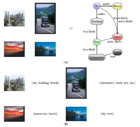
Figure 1: Semantic Image Annotation. (A). During training, we train a function mapping an image to the label semantics. (B). During prediction, we annotate each image a set of labels.

Extending traditional classification techniques to structured prediction is difficult because of the potentially complicated inter-dependencies that may exist among the output variables. If the problem is modeled as a probabilistic graphical model, it is well-known that exact inference over a general graph is NP-hard. Therefore, practical approaches make simplifying assumptions about the dependencies among the output variables in order to simplify the graph structure and maintain tractability. Examples include maximum entropy Markov models (MEMMs) (Mccallum et al, 2000), conditional random fields (CRFs) (Lafferty et al, 2001; Quattoni et al, 2004), max-margin Markov networks (M3Ns) (Taskar et al, 2004) and structured support vector machines (SSVMs) (Tsochantaridis et al, 2004). These approaches typically restrict the tree-width of the graph so that the Viterbi algorithm or the junction tree algorithm can still be efficient.

On the other hand, there has been much research on fast approximate inference for complicated graphs based on, e.g., Markov chain Monte Carlo (MCMC), variational inference, or combinations of these methods. In general, MCMC is slow, particularly for graphs with strongly coupled variables. Good heuristics have been developed to speed up MCMC, but they are highly dependent on graph structure and associated parameters (Doucet et al, 2000). Variational inference is another popular approach where a complicated distribution over $\bf Y$ is approximated with a simpler distribution so as to trade accuracy for speed. For example, if the variables are assumed to be independent, one obtains the mean field algorithm. A Bethe energy formulation yields the loopy belief propagation (LBP) algorithm (Yedidia et al, 2005). If a combination of trees is considered, one obtains the tree-reweighted sum-product algorithm (Wainwright et al, 2005a). One can also relax the higher-order marginal constraints to obtain a linear programming algorithm (Wainwright et al, 2005b). The lesser the dependency constraints, the less accurate these inference algorithms become, and the faster their speed. However, the sacrificed accuracy in inference could be detrimental to learning. For example, mean field can produce highly biased estimates, and loopy belief propagation might even cause the learning algorithm to diverge
 (Kulesza and Pereira, 2007).

Long-range dependencies and complicated graphs are necessary to accurately and precisely represent semantic knowledge. Unfortunately, the approaches discussed above all operate under the assumption that one cannot avoid the trade-off between the representational power and computational efficiency.

In this paper, we propose large margin sigmoid belief networks (LMSBNs) and large margin Boltzmann machines (LMBMs), two new models for structured prediction. We provide a theoretical analysis tool to derive the generalization bounds for both of them. Most importantly, LMSBNs allow fast inference for arbitrarily complicated graph structures. Inference is based on a branch-and-bound (BB) technique that does not depend on the dependency structure of the graph and exhibits the interesting property that the better the fit of the model to the data, the faster the inference procedure.

Section 2 describes both LMSBNs and LMBMs. We present learning algorithms for both and the fast BB inference algorithm for LMSBNs. LMBMs, being undirected, rely on traditional inference algorithms.

Section 4 applies both LMSBNs and LMBMs to the semantic image annotation problem using a fully-connected graph structure. We empirically study the performance of the BB inference algorithm and illustrate its efficiency and effectiveness. We present results from experiments on a benchmark dataset which demonstrate that LMSBNs outperform current state-of-the-art methods for image annotation based on kernels and threshold-tuning.

2 Large Margin Sigmoid Belief Networks and Large Margin Boltzmann Machines

The sigmoid belief network (SBN) (Neal, 1992) and Boltzmann machine (BM) (Hinton and Sejnowski, 1983) are a special type of Bayesian network and a special type of Markov random field respectively, and are defined as follows:

Definition 1

A Boltzmann machine is an undirected graph $G=({\bf V},E)$, where $\bf V$ is the set of random variables with size $K=|\bf V|$, $E$ is the set of undirected edges. The joint likelihood is defined as:

$$\Pr({\bf V}|{\bf w}) = e^{\frac{1}{2}\sum_{i}z_{i}}/\sum_{\bf V}e^{\frac{1}{2}\sum_{i}z_{i}}$$ (1)

$$z_{i} = \sum_{j:(V_{i},V_{j})\in E}w_{ij}v_{i}v_{j}+w_{i}v_{i}$$

where $Z$ is the normalization constant.

Definition 2

A sigmoid belief network is a directed acyclic graph $G=({\bf V},E)$, where $\bf V$ is the set of random variables with size $K=|\bf V|$, $E$ is the set of directed edges. $(V_{j},V_{i})$ represents an edge from $V_{j}$ to $V_{i}$. For each node $V_{i}$, its parents are in the set $pa(V_{i})=\{V_{j}|(V_{j},V_{i})\in E\}$. The joint likelihood is defined as:

$$\Pr({\bf V}|{\bf w}) = \prod_{i=1}^{K}\Pr(V_{i}|pa(V_{i}),{\bf w})$$ (2)

$$\Pr(V_{i}|pa(V_{i}),{\bf w}) = \frac{1}{1+e^{-z_{i}}}$$

$$z_{i} = \sum_{j:V_{j}\in pa(V_{i})}w_{ij}v_{i}v_{j}+w_{i}v_{i}$$

In BMs, the edges are undirected, so the feature $v_{i}v_{j}$ appears in both $z_{i}$ and $z_{j}$. In SBNs, the edges are directed, so the feature $v_{i}v_{j}$ appears in either $z_{i}$ or $z_{j}$, but not both. One can generalize the function $z_{i}$ to utilize high order features over a set of variables. In probabilistic graphical models, this set is referred to as a clique. In SBNs or BMs, the features are defined as a product of all variables in the clique. For example, $C_{1}=\{V_{1},V_{2},V_{3}\}$ is a 3rd order clique, $f_{1}=v_{1}v_{2}v_{3}$. The edges are 2nd order cliques, e.g., $C_{2}=\{V_{1},V_{2}\}$, $f_{2}=v_{1}v_{2}$. The first order cliques are the variable themselves, e.g., $C_{3}=\{V_{1}\}$, $f_{3}=v_{1}$. When the variables take values $\{-1,1\}$, the feature function is also known as the parity function or the XOR function. Therefore, a SBN or BM softly encodes a Boolean function via an AND-of-XOR expansion, which provides a flexible way to encode human expert knowledge into the model. Without ambiguity, we simplify the representation of $z_{i}$ to be $z_{i}=\sum_{j}w_{ij}f_{j}$, where the summation is taken over all cliques that include variable $V_{i}$. For SBNs, We require that all the variables in each clique $C_{j}$ other than $V_{i}$ must be parents of $V_{i}$. This requirement insures that the underlying graph is acyclic, and each $C_{j}$ is used in one $z_{i}$.

In the structured prediction setting, the problem involves an input vector $\bf X$, and the joint probability over all $\bf Y$ is conditioned on $\bf X$, i.e., $\Pr({\bf Y}|\bf X,w)$. Note that $z_{i}$ is defined for each $Y_{i}$ although the cliques include both $\bf X$ and $\bf Y$.

When there is only one output variable, i.e. $K=1$, the conditional likelihoods of both SBNs and BMs become the same, i.e., $\Pr(Y=y|{\bf x};{\bf w})=\frac{1}{1+e^{-z}}$, where $z=y\sum_{j}w_{j}\phi_{j}({\bf x})$. The features are $f_{j}({\bf x},y)=y\phi_{j}({\bf x})$. This is the well known logistic regression (LR) with a loss function $L(y,{\bf x,w})=\log(1+e^{-z})$. In fact, a SBN can be considered as a product of LRs according to a topological order over the graph. The overall loss function is then $L({\bf y,x,w})=\sum_{i}\log(1+e^{-z_{i}})$. A BM needs normalization over all $\bf Y$, the loss function usually can not be factorized locally that puts some challenge on learning.

To facilitate the derivation of a fast inference algorithm for LMSBNs and a fast learning algorithm for LMBMs, we use a hinge loss, $[1-z]_{+}=\max(0,1-z)$ to approximate the log-loss $\log(1+e^{-z})$. We call the resulting SBN a large margin sigmoid belief network (LMSBN) and the resulting BM a large margin Boltzmann machine (LMBM). The approximations are presented in Remark 3. The approximation of LMBM is similar to pseudo likelihood approximation of a Markov random field. The only difference is the extra regularization. In the latter section, we will show that this regularizer is crucial for LMBMs to generalize well. Note that for LMSBNs, each feature $f_{j}$ only appears in one $z_{i}$, but for LMBMs, each feature $f_{j}$ appears in all $z_{i}$ where $Y_{i}\in C_{j}$.

Remark 3

$$L_{SBN}({\bf y,x,w}) \leq L_{LMSBN}({\bf y,x,w})+Kb$$

$$L_{BM}({\bf y,x,w}) \leq L_{LMBM}({\bf y,x,w})+Kb+g(\bf x)\left\|\bf w\right\|$$

$$L_{LMSBN}({\bf y,x,w}) = L_{LMBM}({\bf y,x,w})=\sum_{i}[1-z_{i}]_{+}$$ (3)

$$z_{i} = \sum_{j:Y_{i}\in C_{j}}w_{j}f_{j}$$

$$b \log(e+e^{-1})$$ ⁼

Proof

From Figure 2, it is easy to verify that $\log(1+e^{-z})\leq[1-z]_{+}+b$, which leads to the first upper bound for SBN. For BM, because the features involves multiple variables ${Y_{i}}$ appear in all corresponding ${z_{i}}$, which makes the upper bounding much harder. Here we prove the second upper bound as follows:

$$L_{BM}({\bf y,x,w})$$ (4)

$$= -\frac{1}{2}\sum_{i}z_{i}+\log\sum_{\bf Y}e^{\frac{1}{2}\sum_{i}z_{i}}$$

$$= -\frac{1}{2}\sum_{i}z_{i}+\log\sum_{{\bf Y}\setminus Y_{1}}e^{\frac{1}{2}\sum_{i\neq 1}z_{i}}\sum_{Y_{1}=\{-y_{1},y_{1}\}}e^{\frac{1}{2}z_{1}}$$

$$\leq -\frac{1}{2}\sum_{i\neq 1}z_{i}+\log\sum_{{\bf Y}\setminus Y_{1}}e^{\frac{1}{2}\sum_{i\neq 1}z_{i}}e^{[1-z_{1}]_{+}+b}$$

$$\leq -\frac{1}{2}\sum_{i\neq 1}z_{i}+\log\sum_{{\bf Y}\setminus\{Y_{1},Y_{2}\}}e^{\frac{1}{2}\sum_{i\neq\{1,2\}}z_{i}}$$

$$\quad\sum_{Y_{2}=\{-y_{2},y_{2}\}}e^{\frac{1}{2}z_{2}}e^{[1-z_{1}]_{+}+b}$$

$$\leq -\frac{1}{2}\sum_{i\neq\{1,2\}}z_{i}+\log\sum_{{\bf Y}\setminus\{Y_{1},Y_{2}\}}e^{\frac{1}{2}\sum_{i\neq\{1,2\}}z_{i}}$$

$$\quad e^{[1-z_{2}]_{+}+[1-z_{1}]_{+}+2b+g_{1}({\bf x})\sum_{j:Y_{1},Y_{2}\in C_{j}}w_{j}^{2}}$$

$$\leq \sum_{i}[1-z_{i}]_{+}+Kb+g({\bf x})\sum_{j:C_{j}\in\mathcal{C}^{\prime}}w_{j}^{2}$$

since the hinge loss for $Y_{1}$ also contains $Y_{2}$, when the partition function marginalizes $Y_{2}$, we have to relax the summation with a term proportional to the norm of the weights whose corresponding cliques include both $Y_{1}$ and $Y_{2}$. This relaxation is represented by $g_{1}({\bf x})\sum_{j:Y_{1},Y_{2}\in C_{j}}w_{j}^{2}$, where $g_{1}$ is a constant determined by $\bf x$. After the whole partition function being relaxed, the upper bound contains a regularizer on all the weights whose corresponding cliques include at least two output $Y$. The set of all these cliques is $\mathcal{C}^{\prime}$. ∎

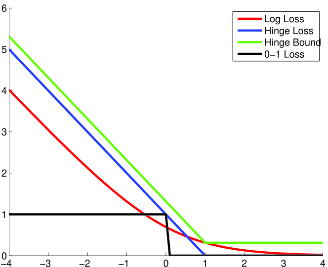
Figure 2: Losses and upper bound

Output values are predicted by minimizing the loss function, as shown in Equation 5 below. With an $\ell_{2}$ norm regularization on the weights $\bf w$, the training problem for LMSBNs is defined as in Equation 6 below. Note that, for LMBMs, there is an extra $\ell_{2}$ regularization on the weights among the output $\bf Y$, but no regularization on the weights for individual $\bf Y$ or between $\bf X$ and $\bf Y$.

$$\hat{\bf y} = \arg\min_{\bf y}L(\bf y,x,w)$$ (5)

$$\hat{\bf w} = \arg\min_{\bf w}\frac{1}{N}\sum_{l=1}^{N}L({\bf y}_{l},{\bf x}_{l},{\bf w})+R(\bf w)$$ (6)

LMDBNs $$: R(\bf w)\equiv\lambda\left\|\bf w\right\|_{2}^{2}$$

LMBMs $$: R(\bf w)\equiv\lambda\left\|\bf w\right\|_{2}^{2}+\lambda\eta_{0}\left\|{\bf w}_{\mathcal{C}^{\prime}}\right\|_{2}^{2}$$

2.1 Generalization Bound

One major concern of structured prediction, as well as all classification problems, is generalization performance. Generalization performance for structured prediction has not been as well studied as for binary and multi-class classification (Taskar et al, 2004; Tsochantaridis et al, 2004; Daumé III et al, 2009). Both Taskar et al and Tsochantaridis et al employed the maximum-margin approach that builds on binary support vector machines (SVMs). Generalization performance can be addressed by an upper bound on the prediction errors. However, the derivation of the bound is specifically restricted to the loss function they use, and hard to apply to other loss functions. Daumé III et al consider a sequential decision approach that solves the structured prediction problem by making decisions one at a time. These sequential decisions are made multiple times, and the output is obtained by averaging all results. The generalization bound is analyzed in terms of all these binary classification losses. One major drawback of this approach is that the averaged losses for the averaged classifiers need a large number of iterations to converge. Even if it converges, the bound is still loose compared to the bound we presented. We will discuss this further in Section 3.

In this section, we provide a general analysis tool for both single variable classification and structured prediction that allows arbitrary loss functions and holds tight. We first need the following threshold theorem:

Theorem 4

Assuming ${\bf X,Y}\sim\mathcal{D}$,if  $\forall{\bf y}\neq\hat{\bf y}$, $\exists T>0$, s.t. $L({\bf x,y,w})>T$, then

$$\Pr(\hat{\bf y}\neq{\bf y}|{\bf w})\leq\frac{1}{T}\mathbb{E}_{\mathcal{D}}[L({\bf x,y,w})]$$ (7)

Proof

$$\Pr(\hat{\bf y}\neq{\bf y}|{\bf w}) = \mathbb{E}_{\mathcal{D}}[\textbf{1}(\hat{\bf y}\neq{\bf y})]$$

$$\leq \mathbb{E}_{\mathcal{D}}[\mathcal{H}(L({\bf x,y,w})-T)]$$

$$\leq \frac{1}{T}\mathbb{E}_{\mathcal{D}}[L({\bf x,y,w})]$$

The function $\textbf{1}(z)$ is the indicator function that is 1 when $z$ is true and 0 for false. $\mathcal{H}(z)$ is the Heaviside function that is 1 for $z\geq 0$ and 0 otherwise. The last inequality comes from the fact that $\mathcal{H}(z-T)\leq\frac{z}{T}$.

This threshold theorem allows one to discuss the prediction error bounds for any number of outputs with any loss function. For example, for logistic regression (LR), $L=\log(1+e^{-z})>\log 2$ whenever a mistake is made, so the threshold $T$ for LR is $\log 2$. In Adaboost (Zhang, 2001), $L=e^{-z}>1$ whenever it makes a mistake, so $T=1$. For SSVMs, $L=[1-\max_{{\bf y^{\prime}}\neq{\bf y}}(z({\bf y,x,w})-z({\bf y^{\prime},x,w}))]_{+}>1$ when it makes a mistake, so $T$ is again $1$. Then the prediction errors for all these classifiers are upper bounded by the expected loss divided by the threshold $T$.

According to this theorem, the goal of all classification tasks is to find the hypothesis that predict with an expected loss as low as possible. On the other hand, for LMSBNs, there is a fast inference algorithm whose performance directly dependents on this quantity. The smaller the expected loss, the faster the inference. For both of the above reasons, the log-loss and exponential-loss are unfavorable because they are usually larger than zero even if the model fits the data well. Therefore, we choose the hinge loss as the loss function for both LMSBNs and LMBMs.

The threshold for LMBMs is given in Remark 5, and the threshold for LMSBNs is given in Remark 6. For a tight bound, the threshold should be large enough, so for LMBMs, we need to constrain the weights among the output variables. In other words, if the coupling between outputs is stronger than the coupling between an output and an input, then the possibility of overfitting increases. This also explains why the approximate loss of LMBMs contains regularizations for the coupling weights among the output variables. However, for LMSBNs, the threshold is always $1$. Generally speaking, LMSBNs can be expected to generalize better than LMBMs.

Remark 5

For LMBMs, $T=\min_{i}[\gamma-g({\bf x})\sum_{j:C_{j}\in\mathcal{C}^{\prime}}w_{j}^{2}]_{+}$, for some $g$.

Proof

For any $y_{i}\neq\hat{y_{i}}$, we have $[1-z_{i}]_{+}=[1-A_{0}-A_{1}]_{+}$,$[1-\hat{z}_{i}]_{+}=[1-A_{0}-A_{2}]_{+}$ where $A_{0}=\sum_{j:f_{j}=\hat{f}_{j}}w_{j}f_{j}$,
$A_{1}=\sum_{j:f_{j}\neq\hat{f}_{j}}w_{j}f_{j}$,
$A_{2}=\sum_{j:f_{j}\neq\hat{f}_{j}}w_{j}\hat{f}_{i}$. Since all $\bf y$ takes $\{-1,+1\}$, so $A_{2}=-A_{1}$, and $[1-\hat{z}_{i}]_{+}=[1-A_{0}+A_{1}]_{+}$.
If $A_{1}<0$, we have $L>[1-z_{i}]_{+}>[1-A_{0}]_{+}$. Otherwise, $L>\hat{L}>[1-\hat{z}_{i}]_{+}>[1-A_{0}]_{+}$. So $L>[1-\sum_{j:f_{j}=\hat{f}_{j}}w_{j}f_{j}]_{+}$. We can further loosen it to $L>\min_{i}[1-g({\bf x})\sum_{j:C_{j}\in\mathcal{C}^{\prime}}w_{j}^{2}]_{+}$.∎

Remark 6

For LMSBNs, $T=1$

Proof

Pick the first $Y_{i}$ in the topological order that does not equal the optimal value, i.e. $y_{i}\neq\hat{y}_{i}$ and $\forall y_{j}\prec y_{i},y_{j}=\hat{y}_{j}$. Let $L_{i}=[1-z_{i}]_{+}$ and $\hat{L_{i}}=[1-\hat{z}_{i}]_{+}$. Since $Y$ takes values $\{-1,1\}$ and only $y_{i}\neq\hat{y}_{i}$ in $z_{i}$, it is easy to verify that $z_{i}=-\hat{z}_{i}$. So, we have $L_{i}=[1+\hat{z}_{i}]_{+}$. If $\hat{z}_{i}>0$, we have $L\geq L_{i}\geq 1$. Otherwise, $L\geq\hat{L}\geq\hat{L_{i}}\geq 1$.∎

We assume all data are drawn from the same unknown distribution $\mathcal{D}$. Since $\mathcal{D}$ is unknown, one can only minimize the empirical risk rather than the expected risk. A fast convergence rate of the empirical objective to the expected one was proved in (Shalev-Shwartz et al, 2008) for the single output variable case. We can extend it to the general structured output case by providing a structured Rademacher complexity bound, as shown in Lemma  7.

Lemma 7

Let $\mathcal{F}=\{{\bf x,y}\mapsto L(\bf x,y,w)\}$,
$\mathcal{F}_{i}=\{{\bf x,y}\mapsto\sum_{j:Y_{i}\in C_{j}}w_{j}f_{j}\}$, $\phi(z)=[1-z]_{+}$. We have

$$\mathbb{E}\left[\sup_{h\in\mathcal{F}}\left(\mathbb{E}h-\hat{\mathbb{E}}_{N}h\right)\right]\leq\sum_{i}\mathcal{R}_{N}(\phi\circ\mathcal{F}_{i})$$

Proof

$$\mathbb{E}\left[\sup_{h\in\mathcal{F}}\left(\mathbb{E}h-\hat{\mathbb{E}}_{N}h\right)\right]$$

$$\leq \mathbb{E}\left[\sup_{h\in\mathcal{F}}\frac{1}{N}\sum_{l}\left(h({\bf x}_{l}^{\prime},{\bf y}_{l}^{\prime})-h({\bf x}_{l},{\bf y}_{l})\right)\right]$$

$$\leq \mathbb{E}\left[\sum_{i}\sup_{h_{i}^{\prime}\in\phi\circ\mathcal{F}_{i}}\frac{1}{N}\sum_{l}\left(h_{i}^{\prime}({\bf x}_{l}^{\prime},{\bf y}_{l}^{\prime})-h_{i}^{\prime}({\bf x}_{l},{\bf y}_{l})\right)\right]$$

$$= \sum_{i}\mathcal{R}_{N}(\phi\circ\mathcal{F}_{i})$$

Here $\mathcal{R}_{N}$ is the Rademacher complexity (Bartlett and Mendelson, 2003) of sample size $N$. See (Bartlett and Mendelson, 2003) for details on the notation.∎

Together with Lemma 7 and Corollary 4 in (Shalev-Shwartz et al, 2008), we can now derive a generalization bound as in Theorem 8.

Theorem 8

Let $\mathcal{L}({\bf w})=\mathbb{E}_{\mathcal{D}}[L(\bf x,y,w)]$, ${\bf w}_{o}=\arg\inf_{\bf w}\mathcal{L}({\bf w})$. Assuming $\sum_{j}f_{j}^{2}<B^{2}$, for any $\delta>0$, with probability $1-\delta$ over the sample size $N$, if $\lambda=c\frac{B\sqrt{d/\delta}}{\left\|{\bf w}_{o}\right\|_{2}\sqrt{N}}$, where $c$ is a constant, we have

$$\Pr(\hat{\bf y}\neq{\bf y}|\hat{\bf w}) \leq \frac{1}{T}\mathcal{L}(\hat{\bf w})$$

$$\mathcal{L}(\hat{\bf w}) \leq \mathcal{L}({\bf w}_{o})+O\left(B\left\|{\bf w}_{o}\right\|_{2}\sqrt{\frac{\log{(d/\delta)}}{N}}\right)$$

The basic idea of the structured Rademacher complexity is to bound the whole functional space by a combination of the Rademacher complexity of each subspaces. For LMBMs, a $f_{j}$ will be shared by all $z_{i}$ where $Y_{i}\in C_{j}$. So the subspaces overlap with each other, and the overall Rademacher complexity counts the features multiple times while $B$ counts only once. Therefore the generalization bound is loosened by $\sqrt{d}$, where $d$ is the maximum clique size. The more complicated the graph, the larger the $d$. For LMSBNs, each feature only appears in one subspace, so $d$ is always $1$. Hence the bound for LMSBNs is tighter than for LMBMs.

Furthermore, the bound given above is better than the PAC-Bayes bound of SSVMs and is not affected by the inference algorithm. For SSVMs, when there is no cheap exact inference algorithm available, the PAC-Bayes bound becomes worse due to the extra degrees of freedom introduced by relaxations (Kulesza and Pereira, 2007), leading to potentially poorer generalization performance.

2.2 Learning Algorithm

For LMSBNs, the learning problem defined in Equation 6 can be decomposed into $K$ independent optimization problems. Each of them can be solved efficiently by any of the modern fast solvers such as the dual coordinate descent algorithm (Hsieh et al, 2008) (DCD), the primal stochastic gradient descent algorithm (PEGASOS) (Shalev-Shwartz et al, 2007; Bottou and Bousquet, 2008) or the exponentiated gradient descent algorithm (Collins et al, 2008). For LMBMs, the weights are shared in multiple $z_{i}$, one has to optimize the whole objective simultaneously. Similar to (Hsieh et al, 2008), we give a dual coordinate descent based optimization algorithms for LMBMs.

Consider the following primal optimization problem:

$$\min_{\bf w,\xi} \frac{1}{2}\sum_{j}\eta_{j}w_{j}^{2}+\frac{1}{\lambda N}\sum_{il}\xi_{il}$$

subject to $$\sum_{j:Y_{i}\in C_{j}}w_{j}f_{jl}\geq 1-\xi_{il}$$

$$\xi_{il}\geq 0$$

where $\eta_{j}=1$ if $w_{j}$ is not extra regularized; otherwise, $\eta_{j}=1+\eta_{0}$. The index $l$ represents each training data. Let $\alpha_{il}$ and $\beta_{il}$ be Lagrange multipliers. Then, we have the Lagrangian:

$$\mathbb{L}({\bf w},\xi,\alpha,\beta) = \frac{1}{2}\sum_{j}\eta_{j}w_{j}^{2}+\frac{1}{\lambda N}\sum_{il}\xi_{il}-\sum_{il}\beta_{il}\xi_{il}-$$

$$\sum_{il}\alpha_{il}(\sum_{j:Y_{i}\in C_{j}}w_{j}f_{jl}-1+\xi_{il})$$

We optimize $\mathbb{L}$ with respect to $\bf w$ and $\xi$:

$$\frac{\partial\mathbb{L}}{\partial w_{j}} = \eta_{j}w_{j}-\sum_{l}\sum_{i:Y_{i}\in C_{j}}\alpha_{il}f_{jl}=0$$

$$\frac{\partial\mathbb{L}}{\partial\xi_{il}} = \frac{1}{\lambda N}-\alpha_{il}-\beta_{il}=0$$

Substituting for $\bf w$ and $\xi$, we have the dual objective:

$$\mathbb{L}_{\alpha} = \frac{1}{2}\sum_{j,l,l^{\prime}}\sum_{i:Y_{i}\in C_{j}}\sum_{i^{\prime}:Y_{i^{\prime}}\in C_{j}}\alpha_{il}\alpha_{i^{\prime}l^{\prime}}Q_{jll^{\prime}}-\sum_{il}\alpha_{il}$$

where $Q_{jll^{\prime}}=\frac{f_{jl}f_{jl^{\prime}}}{\eta_{j}^{2}}$. The dual coordinate descent algorithm picks $\alpha_{il}$ one at a time and optimizes the dual Lagrangian with respect to this variable. The resulting algorithm is described in Algorithm 1.

Algorithm 1 The dual coordinate descent algorithm for large margin Boltzmann machines

0:  $\left\{f_{jl}\right\},\left\{Q_{jll}\right\},\lambda,N$

0:  $\bf w$

1:  $\alpha\leftarrow 0,{\bf w}\leftarrow 0$

2:  while $\alpha$ is not optimal do

3:     for all $\alpha_{il}$ do

4:        $\alpha_{o}\leftarrow\alpha_{il}$

5:        $G=\sum_{j:Y_{i}\in C_{j}}w_{j}f_{jl}-1$

6:        $PG=\left\{\begin{array}[]{cc}\min(G,0)&\alpha_{o}=0,\\ \max(G,0)&\alpha_{o}=\frac{1}{\lambda N},\\ G&0<\alpha_{o}<\frac{1}{\lambda N}\\ \end{array}\right.$

7:        if $|PG|\neq 0$ then

8:           $\alpha_{il}\leftarrow\min(\max(\alpha_{o}-\frac{G}{\sum_{j:Y_{i}\in C_{j}}Q_{jll}},0),\frac{1}{\lambda N})$

9:           $w_{j}\leftarrow w_{j}+(\alpha_{il}-\alpha_{o})f_{jl},\forall j:Y_{i}\in C_{j}$

10:  return $\bf w$

2.3 Inference Algorithm

In this section, we propose a simple and efficient inference algorithm (Algorithm 2) to solve the prediction problem in Equation 5 for LMSBNs. According to the topological order of the graph, we branch on each $Y_{i}$, and compute $z_{i}$ with $\bf x$ and all of its parents $y_{j}$. We first try the value of $y_{i}$ that makes $z_{i}>0$, i.e., the left branch in the algorithm, then the right branch with the opposite value of $y_{i}$. During this search, we keep an upper bound initialized to a parameter $S\geq 1$. Whenever the current objective is higher than the upper bound, we backtrack to the previous variable. The search terminates before $K^{S}$ states of $\bf Y$ have been visited.

Algorithm 2 The Branch and Bound Algorithm for Inference

0:  $\bf x,w$, $S\geq 1$

0:  $\hat{\bf y},UB$

1:  $UB=S$, $i=0$, $\bf U=0$;

2:  while $i>=0$ do

3:     if $i=K$ then

4:        if $U_{K}<UB$ then

5:           $UB=U_{K}$,  $\hat{\bf y}=\bf y$;

6:        $i=i-1$;

7:     else

8:        if Left branch has not been tried then

9:           $y_{i}=\arg\max_{y_{i}}z_{i}$,  $U_{i+1}=U_{i}+[1-z_{i}]_{+}$;

10:        else if Right branch has not been tried then

11:           $y_{i}=-y_{i}$, $U_{i+1}=U_{i}+[1+z_{i}]_{+}$;

12:        if $U_{i+1}\geq UB$ or both branches have been tried then

13:           $i=i-1$;

14:        else

15:           $i=i+1$;

The following theorem shows that with a high probability, the above algorithm computes the optimal values in polynomial time:

Theorem 9

For any $S\geq 1$, the BB algorithm reaches the optimal values before $O(K^{S})$ states are visited with a probability at least $1-\frac{1}{S}\mathcal{L}({\bf w})$.

Proof

During the search, if we branch on the right, the hinge loss $[1+z_{i}]_{+}$ is greater than 1. So, for a given $\bf x$, if the true objective $L<S$, the optimal objective $\hat{L}<L<S$ as well, and the optimal path contains at most $S$ right branches. Since the BB algorithm always searches the left branch first, the optimal path will be reached before $\sum_{i=0}^{S-1}\left(\begin{array}[]{c}i\\ K\end{array}\right)\leq O(K^{S})$ states have been searched. According to the Markov inequality, $\Pr(L<S)=1-\Pr(L>S)\geq 1-\frac{1}{S}\mathcal{L}(\bf w)$.

The BB algorithm adjusts the search tree according to the model weights. Through training, optimal paths are condensed to the low energy side, i.e., the left side of the search tree with a high probability. This probability is directly related to the expected loss with respect to the given data distribution. We therefore label the BB algorithm a data-dependent inference algorithm. Most popular inference algorithms for exact or approximate inference depend on graph complexity: the more complicated the graph, the slower the inference. This trade-off diminishes the applicability of these algorithms and presents researchers with the difficult problem of selecting a (possibly sub-optimal) graph structure that balances the accuracy and the efficiency. The BB algorithm for LMSBNs circumvents this trade-off and allows arbitrary complicated graphs without sacrificing computational efficiency. In fact, if a particular complicated graph yields a smaller expected loss, the BB algorithm in turn runs even faster.

It is well-known that for NP-hard problems, there may be many instances that can be solved efficiently. The area of speedup learning focuses on learning good heuristics to speedup problem solvers. The approach presented here can be regarded as a novel method for speedup learning (Tadepalli and Natarajan, 1996) and demonstrates that the experience gained during training can speedup a problem solver significantly.

The BB algorithm is specifically designed for LMSBNs, a directed graphical model. For undirected models, the BB algorithm does not guarantee a polynomial time complexity with a high probability. Indeed, we observe an exponential time complexity when it is applied to LMBMs. For the undirected models including SSVMs and LMBMs, we implement a convex relaxation-based linear programming (LP) (Wainwright et al, 2005b). Note that although LMBMs don’t have a fast inference algorithm, unlike SSVMs, the learning is not affected by the inference algorithm. In the experiments section, we will show that LMBMs outperforms SSVMs.

The BB algorithm differs from other search-based decoding algorithms, e.g., beam search and best first search (Abdou and Scordilis, 2004), in several aspects. First, those search algorithms typically prune the supports of maximum cliques that can grow exponentially. On one hand, the pruning can lead to misclassification quickly if backtracking is not implemented. On the other hand, the number of remaining states might still be large so that the inference is still slow. Furthermore, even if a backtracking procedure is implemented, unlike the BB algorithm for LMSBNs, there are still no guaranteed heuristics that can prune the states efficiently and correctly.

To demonstrate the efficiency and the data dependency property, we run the algorithms on the test data of RCV1-V2 (a text categorization dataset) with a trained model and a random untrained model. The running times are collected by varying the number of output variables. The CPU time is measured on a 2.8Ghz Pentium4 desktop computer.

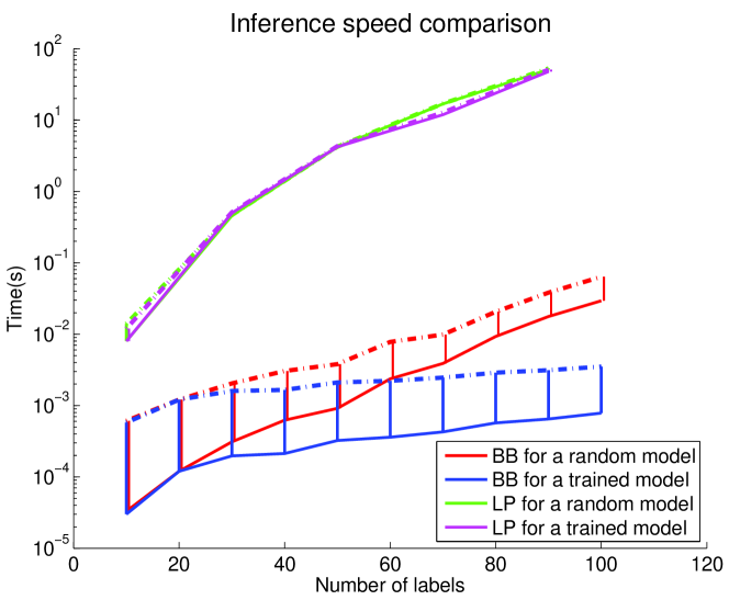
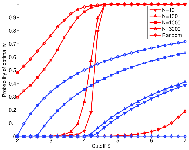
Figure 3: Upper graph. Running time comparisons of LP and BB algorithms on the test dataset of RCV1-V2. The dashed lines are 1 standard deviation above the mean. The time axis is log-scaled. Lower graph. Accuracy and data distribution dependency. The more the training data, the more accurate and faster the prediction. The corresponding estimated theoretical lower bounds are plotted in blue.

The upper graph in Figure 3 demonstrates that the BB algorithm performs several orders of magnitude faster than LP. In this experiment, $S$ is set to a very large value such that the solution from BB is guaranteed to be the optimal solution. The running time of LP with respect to the number of output variables does not vary from a trained model to a random untrained model, but the running time of BB changes significantly. For the random untrained model, the BB algorithm demonstrates an exponential time complexity with respect to the number of output variables. However, after training, the running time of the BB algorithm scales up much more slowly.

This observation underscores the data distribution dependent property of BB, i.e., the better the model fits the data, the faster BB performs. We illustrate this property further by a second experiment. In this experiment, the probability of the BB algorithm reaching the optimal values is plotted by varying the cutoff threshold $S$. According to Theorem 9, $S$ reflects the running time overhead for the BB algorithm. We compare this curve for several models, namely, a random model and models trained with 10, 100, 1000, and 3000 training instances respectively. The lower graph in Figure 3 shows a significant improvement for the trained models over the random untrained model. Moreover, with more and more training instances, more and more test instances can be predicted exactly and quickly. In the same figure, we also plot the corresponding theoretical lower bounds estimated from the testing dataset (blue lines). The lower graph of Figure 3 verifies Theorem 9 empirically.

Due to the fast and accurate inference algorithm for LMSBNs, we can start with the most complicated graph structure, i.e., a fully connected model. The linear form of $z_{i}$ can be generalized to high order features. Moreover, the kernel trick can be applied to augment the modeling power. The only thing one needs to concern is to minimize the expected loss as much as possible because the small expected loss guarantees not only a high prediction accuracy but also a fast inference.

3 Related Models

Most maximum margin estimated structured prediction models, e.g., SSVMs (Tsochantaridis et al, 2004), maximum margin Markov networks (M3Ns) (Taskar et al, 2004), Maximum margin Bayesian networks (M2BNs) (Guo et al, 2005) and conditional graphical models (CGMs) (Perez-Cruz et al, 2007) adopt a min-max formulation as shown below:

$$\min_{\bf w} \frac{1}{2}\left\|\bf w\right\|^{2}+\frac{1}{\lambda N}\sum_{l}[\Delta({\bf y}_{l},{\bf y})-m({\bf x}_{l},{\bf y}_{l};\bf w)]_{+}$$ (8)

$$m({\bf x}_{l},{\bf y}_{l};{\bf w}) = \max_{{\bf y}\neq{\bf y}_{l}}\Psi({\bf x}_{l},{\bf y}_{l};{\bf w})-\Psi({\bf x}_{l},{\bf y};{\bf w})$$

where $\Psi$ is the compatibility function derived from a probabilistic model, and $m$ is the margin function.

The embedded maximization operation potentially induces an exponential number of constraints. This exponential number of constraints makes optimization intractable. In M2BNs, the local normalization constraints makes the problem even harder. SSVMs utilize a cutting plane algorithm (Joachims et al, 2009) to select only a small set of constraints. M3Ns directly treat the dual variables as the decomposable pseudo-marginals. When the undirected graph is of low tree-width, both SSVMs and M3Ns are computationally efficient and generalize well. However, for high tree-width, approximate inference has to be used and both the computational complexity and the sample complexity increase significantly (Kulesza and Pereira, 2007; Finley and Joachims, 2008).

CGMs decompose the single hinge loss into a summation of several hinge losses, each corresponding to one feature function, such that the exponential number of combinations is greatly reduced. The decomposition from one hinge loss to multiple hinge loss is similar to LMBMs and LMSBNs. However, CGMs decompose to each feature function. For real problems, not every feature function could be compatible to the data, which leads to a large and trivial upper bound. Therefore, the performance can not be guaranteed.

The large margin estimation by the threshold theorem  4 generalizes the maximum margin estimation approach. As long as the loss function satisfies the threshold theorem, there is a margin function implicitly defined such that minimizing the expected loss maximizes the margins. The traditional log-loss based models, e.g., CRFs and MEMMs, can be discussed under the large margin estimation framework, but the thresholds are possibly small so that the upper bounds become trivial. This suggests that large margin estimated models could generalize better than maximum likelihood estimated models.

For problems like semantic annotation, a low-treewidth graph usually is insufficient to represent the knowledge about the relationships among the labels. The example in Figure 1 illustrates the motivation for a high-treewidth graph. All of the models discussed above lack a fast and accurate inference algorithm for high-treewidth graphs, and are subject to the trade-off between the treewidth and computational efficiency.

To speed up inference for a high-treewidth graphical models, one can use mixture models to represent probabilities. For example, MoP-MEMMs (Rosenberg et al, 2007) extend MEMMs to address long-range dependencies and represent the conditional probability by a mixture model. Wainwright et al uses a mixture of trees to approximate a Markov random fields. Both demonstrate performance gains but one still has to improve inference speed by restricting the number of mixtures.

Another line of research for high-treewidth graphical models uses arithmetic circuits (AC) (Darwiche, 2000) to represent the Bayesian networks. The AC inference is linear in the circuit size. As long as the circuit size is low, the inference is fast. But learning the optimal AC is an NP-hard problem. Similarly, one has to improve inference speed by penalizing the circuit size (Lowd and Domingos, 2008).

The search based structured prediction (SEARN) (Daumé III et al, 2009) takes a different approach than probabilistic graphical models to handle the high tree-width graphs. It solves the structured prediction by making decisions sequentially. The later classifier can take all the earlier decisions as inputs, which is similar to LMSBNs. In fact, the inference can be considered as the initial decision of the BB algorithm. The expected errors caused by this naive inference could be very high. SEARN implements an averaging approach to reduce the expected errors. It trains a set of sequential classifiers for each iteration and outputs the prediction by averaging the decisions made over all iterations. The earlier decisions will be fed into later classifiers, so the later classifiers possibly make fewer mistakes. By averaging over iterations, the expected loss are reduced thereafter. Roughly speaking, the prediction errors will be bounded by this averaged expected loss multiplied by $\log K$. Compared to the bounds of LMBMs and LMSBNs, where the prediction errors are bounded by the minimum expected loss divided by the threshold $T$, the generalization bound of SEARN is rather loose. Furthermore, according to (Daumé III et al, 2009), one needs a large number of iterations to reach that bound which slows down the inference. Therefore, one still has to limit the number of iterations for a faster inference, which might sacrifice the prediction accuracy.

Unlike all the above approaches, LMSBNs possess a very interesting property that one does not have any constraints on the modeling power. The smaller the expected loss, the faster the inference. Usually, one obtains a smaller expected loss by using a more complicated graph. This property leads to a novel approach for structured prediction with high tree-width graphs.

4 Experiments

The performance of LMSBNs was tested on a scene annotation problem based on the Scene dataset (Boutell et al, 2004). The dataset contains 1211 training instances and 1196 test instances. Each image is represented by a 294 dimensional color profile feature vector (based on a CIE LUV-like color space). The output can be any combination of 6 possible scene classes (beach, sunset, fall foliage, field, urban, and mountain).

We compare a fully connected LMSBN with three other methods: binary classifiers (BCs), SSVMs (Finley and Joachims, 2008), threshold selected binary classifiers (TSBCs) (Fan and Lin, 2007). BCs train one classifier for each label and predict independently. For SSVMs, we follow (Finley and Joachims, 2008) to implement a fully connected undirected model with binary features. We implement a convex relaxation-based linear programming algorithm for inference, since in both (Finley and Joachims, 2008) and (Kulesza and Pereira, 2007), the convex relaxation-based approximate inference algorithm was shown to outperform other approximate inference algorithms such as loopy belief propagation and graph cuts (Kolmogorov and Zabih, 2002). TSBCs iteratively tune the optimal decision threshold for each classifier to increase the overall performance with respect to a certain measure, e.g., exact match ratio and F-scores. Many labels in the multi-label datasets are highly unbalanced, leading to classifiers that are biased. TSBCs can effectively adjust the classifier’s precision and recall to achieve state-of-the-art performance. In our comparisons, we borrow the best results from (Fan and Lin, 2007) directly.

We implemented two BCs, a linear BC (BCl) and a kernelized BC (BCk), and three LMSBNs: (1) LMSBNlo is trained with default order, i.e., ascending along the label indices; (2) LMSBNlf is trained with the order selected according to the F-scores of the BC. We sort the variables according to their F-scores of the BC. The higher the F-score, the smaller the index in the order; (3) LMSBNkf is a kernelized model with the same order as LMSBNlf. We also implemented two SSVMs: (1) SSVMhmm is trained by using a first-order Markov chain. It is different from the $SSVM^{hmm}$ package that does not consider all inputs $\bf X$ for each $Y_{i}$. The inference algorithm for SSVMhmm is the Viterbi algorithm; (2) SSVMfull is trained by using a fully connected graph.

We consider three categories of performance measures. The first consists of instance-based measures and includes the exact match ratio (E) (Equation 9) and instance-based F-score (Fsam) (Equation 11). The second consists of label-based measures and includes the Hamming loss (H) (Equation 10) and the macro-F score (Fmac) (Equation 12). The last is a mixed measure, the micro-F score (Fmic) (Equation 13). Fsam calculates the F-score for each instance, and averages over all instances. Fmac calculates the F-score for each label, and averages over all labels. Fmic calculates the F-score for the entire dataset.

$$E = \frac{1}{N}\sum_{l}\textbf{1}({\bf y}_{l}={\bf\hat{y}}_{l})$$ (9)

$$H = \frac{1}{NK}\sum_{li}\textbf{1}(y_{li}\neq\hat{y}_{li})$$ (10)

$$Fsam = \frac{1}{N}\sum_{l}\frac{2\sum_{i}\textbf{1}(y_{li}=\hat{y}_{li}=1)}{\sum_{i}(\textbf{1}(y_{li}=1)+\textbf{1}(\hat{y}_{li}=1))}$$ (11)

$$Fmac = \frac{1}{K}\sum_{i}\frac{2\sum_{l}\textbf{1}(y_{li}=\hat{y}_{li}=1)}{\sum_{l}(\textbf{1}(y_{li}=1)+\textbf{1}(\hat{y}_{li}=1))}$$ (12)

$$Fmic = \frac{2\sum_{il}\textbf{1}(y_{li}=\hat{y}_{li}=1)}{\sum_{il}(\textbf{1}(y_{li}=1)+\textbf{1}(\hat{y}_{li}=1))}$$ (13)

The instance-based measure is more informative if the correct prediction of co-occurrences of labels is important; the label-based measure is more informative if the correct prediction of each label is deemed important.

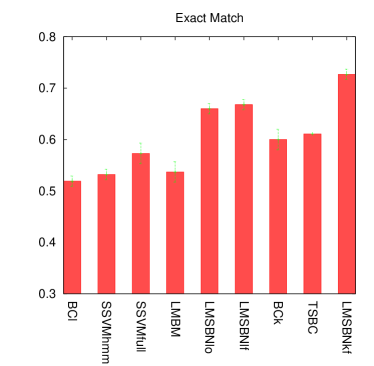
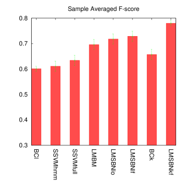
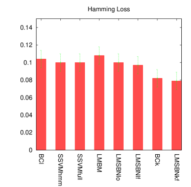
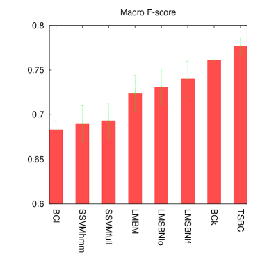
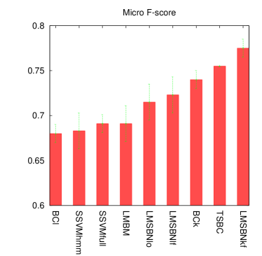
Figure 4: Performance Comparisons. Note: For Hamming loss, the smaller the value, the better the performance.

The results are shown in Figure 4. LMSBNkf consistently performs the best on all measures. Even the LMSBN models without kernels outperform TSBC on instance-based measures.

SSVMhmm performs better than the BCl, but worse than the SSVMfull as expected. The inference speed of BCl is faster than SSVMhmm, which in turn is faster than SSVMfull. This demonstrates the trade-off between modeling power and efficiency.

With the help of kernels, LMSBNkf further outperforms the TSBC on all measures. LMSBNs as proposed in this paper are geared towards minimizing 0-1 errors. Threshold tuning is particularly effective in the case of highly unbalanced labels. An interesting line of research is combining LMSBNs with threshold tuning to further improve the performance.

5 Conclusions

This paper proposes the use of large margin graphical models for fast structured prediction in images with complicated graph structures. A major advantage of the proposed approach is the existence of fast training and inference algorithms, which open the door to tackling very large-scale image annotation problems. Unlike previous inference algorithms for structured prediction, the proposed BB inference algorithm does not sacrifice representational power for speed, thereby allowing complicated graph structures to be modeled. Such complicated graph structures are essential for accurate semantic modeling and labeling of images. Our experimental results demonstrate that the new approach outperforms current state-of-the-art approaches. Future research will focus on applying the framework to annotating parts of images with their spatial relationships, and enhancing the representational power of the model by introducing hidden variables.

References

- Abdou and Scordilis (2004) Abdou S, Scordilis MS (2004) Beam search pruning in speech recognition using a posterior probability-based confidence measure. Speech Communication 42(3-4):409 – 428
- Bartlett and Mendelson (2003) Bartlett PL, Mendelson S (2003) Rademacher and gaussian complexities: risk bounds and structural results. J Mach Learn Res 3:463–482
- Bengio et al (2007) Bengio Y, Lamblin P, Popovici D, Larochelle H, Montr al UD, Qu bec M (2007) Greedy layer-wise training of deep networks. In: In NIPS, MIT Press
- Bottou and Bousquet (2008) Bottou L, Bousquet O (2008) The tradeoffs of large scale learning. In: Platt J, Koller D, Singer Y, Roweis S (eds) Advances in Neural Information Processing Systems, vol 20, NIPS Foundation, pp 161–168
- Boutell et al (2004) Boutell MR, Luo J, Shen X, Brown CM (2004) Learning multi-label scene classification. Pattern Recognition 37:1757–1771
- Carneiro et al (2007) Carneiro G, Chan A, Moreno P, Vasconcelos N (2007) Supervised learning of semantic classes for image annotation and retrieval. IEEE Transactions on Pattern Analysis and Machine Intelligence 29(3):394–410
- Collins et al (2008) Collins M, Globerson A, Koo T, Carreras X, Bartlett PL (2008) Exponentiated gradient algorithms for conditional random fields and max-margin Markov networks. Journal of Machine Learning Research
- Darwiche (2000) Darwiche A (2000) A differential approach to inference in bayesian networks. In: Journal of the ACM, pp 123–132
- Daumé III et al (2009) Daumé III H, Langford J, Marcu D (2009) Search-based structured prediction. Machine Learning Journal
- Doucet et al (2000) Doucet A, Freitas Nd, Murphy KP, Russell SJ (2000) Rao-blackwellised particle filtering for dynamic bayesian networks. In: UAI ’00: Proceedings of the 16th Conference on Uncertainty in Artificial Intelligence, Morgan Kaufmann Publishers Inc., San Francisco, CA, USA, pp 176–183
- Fan and Lin (2007) Fan RE, Lin CJ (2007) A study on threshold selection for multi-label classification. Tech. rep., National Taiwan University
- Finley and Joachims (2008) Finley T, Joachims T (2008) Training structural SVMs when exact inference is intractable. In: ICML ’08: Proceedings of the 25th international conference on Machine learning, ACM, New York, NY, USA, pp 304–311
- Guo et al (2005) Guo Y, Wilkinson D, Schuurmans D (2005) Maximum margin Bayesian networks. In: Uncertainty in Artificial Inteliigence
- Hinton and Sejnowski (1983) Hinton GE, Sejnowski TJ (1983) Optimal perceptual inference. In: CVPR, Washington DC, pp 448–53
- Hsieh et al (2008) Hsieh CJ, Chang KW, Lin CJ, Keerthi SS, Sundararajan S (2008) A dual coordinate descent method for large-scale linear SVM. In: ICML ’08: Proceedings of the 25th international conference on Machine learning, ACM, New York, NY, USA, pp 408–415
- Joachims et al (2009) Joachims T, Finley T, Yu CNJ (2009) Cutting-plane training of structural svms. Mach Learn 77(1):27–59, DOI 10.1007/s10994-009-5108-8
- Kolmogorov and Zabih (2002) Kolmogorov V, Zabih R (2002) What energy functions can be minimized via graph cuts? In: Computer Vision - ECCV 2002: 7th European Conference on Computer Vision, Copenhagen, Denmark, May 28-31, 2002. Proceedings, Part III, pp 185–208