Adaptive Beamforming in Interference Networks via Bi-Directional Training

Abstract

We study distributed algorithms for adjusting beamforming vectors and receiver filters in multiple-input multiple-output (MIMO) interference networks, with the assumption that each user uses a single beam and a linear filter at the receiver. In such a setting there have been several distributed algorithms studied for maximizing the sum-rate or sum-utility assuming perfect channel state information (CSI) at the transmitters and receivers. The focus of this paper is to study adaptive algorithms for time-varying channels, without assuming any CSI at the transmitters or receivers. Specifically, we consider an adaptive version of the recent Max-SINR algorithm for a time-division duplex system. This algorithm uses a period of bi-directional training followed by a block of data transmission. Training in the forward direction is sent using the current beam-formers and used to adapt the receive filters. Training in the reverse direction is sent using the current receive filters as beams and used to adapt the transmit beamformers. The adaptation of both receive filters and beamformers is done using a least-squares objective for the current block. In order to improve the performance when the training data is limited, we also consider using exponentially weighted data from previous blocks. Numerical results are presented that compare the performance of the algorithms in different settings.

I Introduction

The use of multiple antennas in wireless networks offers the promise of mitigating interference and enabling high spectral efficiencies. However achieving these benefits in a decentralized network requires distributed algorithms for coordinating the pre-coding matrices used by each transmitter with minimal overhead. A number of such algorithms have been studied for multiple-input multiple-output (MIMO) interference networks including those in [3, 2, 1] under the assumption that transmitters have perfect channel state information (CSI) for channel matrices to all receivers. Our focus in this work is to relax this assumption and develop adaptive algorithms for time-varying channels without assuming any CSI at the transmitters or receivers.

We consider a MIMO interference network with block fading. Each transmitter uses a rank one pre-coding matrix, i.e. a beamformer, and the receivers are assumed to be linear, with all interference treated as noise, so that the rate is determined by the received signal-to-interference plus noise ratio (SINR). Our objective is to design an adaptive distributed algorithm for updating the precoders and beamformers to maximize the sum-rate while accounting for the needed overhead. To accomplish this, we consider an algorithm for a synchronous time-division duplex (TDD) system that uses one or more bi-directional training periods at the beginning of each block. Each period consists of a forward phase followed by a reverse phase. During the forward phase, all transmitters simultaneously send pilots using their current beamformers and each receiver updates their receive filters. During the backward phase, the receivers transmit pilots, using the current receive filter as a beamformer and the transmitters update their beamformers. The updates during each phase are used to directly adapt the beamformers and receive filters based on a standard least-squares criterion. For a given number of channel users per coherence block, we consider the net throughput achieved after subtracting the channel uses used for training and via numerical results study the effect of varying the training length on these metric. For short coherence blocks, the optimal training length becomes small leading to imprecise estimation and degraded performance. For such settings, we also study a recursive variation of our algorithm based on using exponentially weighted data from previous blocks.

The algorithms we study are inspired by the Max-SINR algorithm in [1]. This algorithm also iterates between transmitter and receiver updates assuming perfect CSI and static channels. Though no convergence proof for this algorithm is given in [1], numerical results show that it has good performance and at high SNRs can achieve the optimal multiplexing gain by successfully aligning the interference at each receiver [4]. Related iterative algorithms (also assuming perfect CSI) are given in [5, 2]. The bi-directional training method presented here is also related to schemes for two-way channel estimation presented in [6, 8, 9, 10, 11, 7]. The key difference here is that we are directly estimating the optimal beamformer and receive filter as opposed to estimating the CSI needed to compute those coefficients.

II System Model

We consider a peer-to-peer wireless network with $K$ transmitter-receiver pairs (henceforth referred to as users) communicating through MIMO links, sharing the same spectrum. Each transmitter has $N_{T}$ antennas, each receiver has $N_{R}$ antennas, and the channel from the $k$-th transmitter to the $j$-th receiver is denoted by a complex matrix $\mathbf{H}_{jk}\in\mathbb{C}^{N_{R}\times N_{T}}$. The channels are assumed to be block-fading, i.e., $\mathbf{H}_{jk}$ remains constant for $L$ symbol periods and jumps to another value for the next $L$ symbols, according to the update

$$\mathbf{H}_{jk}^{(n)}=\alpha\mathbf{H}_{jk}^{(n-1)}+\sqrt{1-\alpha^{2}}\mathbf{W}_{jk}^{(n)}$$ (1)

where $n$ is the block index and $\mathbf{W}_{jk}^{(n)}$ is a matrix with i.i.d complex Gaussian entries having zero mean and the same variance as $\mathbf{H}_{jk}$. (The index $n$ will sometimes be omitted if no confusion results.) We assume that neither transmitters nor receivers have a priori channel information.

For simplicity, we assume each transmitter transmits only one beam to its desired receiver, i.e., the precoding matrix has rank one. The beamforming vector for transmitter $k$ is $\mathbf{v}_{k}\in\mathbb{C}^{N_{T}}$ and satisfies the power constraint $\lVert\mathbf{v}_{k}\rVert^{2}\leq P_{k}^{max}$. The $i$-th received signal vector at the $k$-th receiver in the $n$-th block is then given by

$$\mathbf{y}_{k}(i)=\mathbf{H}_{kk}^{(n)}\mathbf{v}_{k}x_{k}(i)+\sum_{j\neq k}\mathbf{H}_{kj}^{(n)}\mathbf{v}_{j}x_{j}(i)+\mathbf{n}_{k}(i)$$ (2)

where $x_{k}$ is the unit variance data symbol from transmitter $k$ and $\mathbf{n}_{k}$ is the additive noise with covariance matrix $E[\mathbf{n}_{k}\mathbf{n}_{k}^{\operatorname{H}}]=\mathbf{R}_{k}$.

We assume linear receivers, so that the estimated symbol for user $k$ is

$$\widehat{x}_{k}=\mathbf{g}_{k}^{\operatorname{H}}\mathbf{y}_{k}$$ (3)

where $\mathbf{g}_{k}$ is the corresponding receive filter. Given a set of beamformers $\mathbf{v}_{k}$’s and receive filters $\mathbf{g}_{k}$’s, the Signal-to-Interference-plus-Noise Ratio (SINR) for user $k$ can be written as

$$\gamma_{k}=\frac{\lvert\mathbf{g}_{k}^{\operatorname{H}}\mathbf{H}_{kk}^{(n)}\mathbf{v}_{k}\rvert^{2}}{\sum_{j\neq k}\lvert\mathbf{g}_{k}^{\operatorname{H}}\mathbf{H}_{kj}^{(n)}\mathbf{v}_{j}\rvert^{2}+\lvert\mathbf{g}_{k}^{\operatorname{H}}\mathbf{R}_{k}\mathbf{g}_{k}\rvert}.$$ (4)

Ideally, we would like to choose the set of beamforming vectors $\{\mathbf{v}_{k}\}$ and set of receive filters $\{\mathbf{g}_{k}\}$ to maximize the sum rate $\sum_{k=1}^{K}\log(1+\gamma_{k})$ within each block. This is complicated by the assumption that the channels are time-varying, and initially unknown at all nodes. Estimating the channels requires overhead, which reduces the rate, and furthermore, if the channels vary too quickly, then the channel estimates are likely to be inaccurate. Therefore we desire an estimation scheme with minimal overhead, and which adapts to the time-variations of the channel.

III Bi-Directional Optimization: Max-SINR Algorithm

The adaptive bi-directional training scheme to be described is based on the Max-SINR algorithm presented in [1]. That algorithm iteratively optimizes the transmit precoders and receivers, assuming the transmitters/receivers each know their direct- and cross-channel matrices. It consists of the following steps: (i) Fix the precoders and optimize the receivers; (ii) Reverse the direction of transmission, so that the roles of the receiver filters and precoders are swapped, and optimize the precoders (now the receivers).

The optimization criterion in each step is the associated SINR, i.e., in step (i) the receiver for user $k$ is obtained by solving

$$\max_{\mathbf{g}_{k}} \quad\frac{\lvert\mathbf{g}_{k}^{\operatorname{H}}\mathbf{H}_{kk}\mathbf{v}_{k}\rvert^{2}}{\sum_{j\neq k}\lvert\mathbf{g}_{k}^{\operatorname{H}}\mathbf{H}_{kj}\mathbf{v}_{j}\rvert^{2}+\lvert\mathbf{g}_{k}^{\operatorname{H}}\mathbf{R}_{k}\mathbf{g}_{k}\rvert}$$ (5)

$$\mathrm{s.t.} \qquad\qquad\lVert\mathbf{g}_{k}\rVert^{2}=P_{k}^{max}$$ (6)

and in step (ii) the beamformer for user $k$ is updated by solving

$$\max_{\mathbf{v}_{k}} \quad\frac{\lvert\mathbf{v}_{k}^{\operatorname{H}}\mathbf{H}_{kk}^{\operatorname{H}}\mathbf{g}_{k}\rvert^{2}}{\sum_{j\neq k}\lvert\mathbf{v}_{k}^{\operatorname{H}}\mathbf{H}_{jk}^{\operatorname{H}}\mathbf{g}_{j}\rvert^{2}+\lvert\mathbf{v}_{k}^{\operatorname{H}}\mathbf{R}_{k}\mathbf{v}_{k}\rvert}$$ (7)

$$\mathrm{s.t.} \qquad\qquad\lVert\mathbf{v}_{k}\rVert^{2}=P_{k}^{max}.$$ (8)

Although inspired by a duality type of argument, which applies to the uplink/downlink, the max-SINR method does not appear to maximize a particular objective. Hence so far, there is no proof that the algorithm converges. Nevertheless, numerical results show that for the scenario considered (i.e., one beam per user) the Max-SINR algorithm essentially achieves the maximum sum rate over a wide range of SNRs [2].

IV Bi-Directional Training

Maximizing the received SINR in (5) and (7) is equivalent to minimizing the Mean Squared Error (MSE) at the output of the corresponding filter. This leads to an adaptive version in which the MSE is replaced by a Least Squares (LS) cost function. Here we assume that in each step the set of transmitters or the set of receivers synchronously transmit training sequences in each direction.

Specifically, in the $n$-th block, we assume that the transmitters synchronously transmit the sequence of $M$ training symbols given by the matrix $\mathbf{B}^{\operatorname{H}}$ where $\mathbf{B}=[\mathbf{b}_{1}^{\operatorname{H}},\cdots,\mathbf{b}_{K}^{\operatorname{H}}]$ and $\mathbf{b}_{k}$ is the $1\times M$ row vector containing the training symbols $b_{k}(1),\cdots,b_{k}(M)$. The received signal at receiver $k$ is then given by (2) where $x_{k}(i)=b_{k}(i)$. At receiver $k$ the estimated symbol at time $i$ is then $\hat{b}_{k}(i)=\mathbf{g}_{k}^{\operatorname{H}}\mathbf{y}_{k}(i)$. The corresponding sequence of estimated symbols is $\widehat{\mathbf{b}}_{k}=\mathbf{g}_{k}^{\operatorname{H}}\mathbf{Y}_{k}$, where

$$\mathbf{Y}_{k}=\Big{[}\mathbf{y}_{k}(1),\cdots,\mathbf{y}_{k}(M)\Big{]}$$ (9)

The filter $\mathbf{g}_{k}$ is then selected to

$$\min_{\mathbf{g}_{k}}\qquad\lVert\mathbf{b}_{k}-\mathbf{g}_{k}^{\operatorname{H}}\mathbf{Y}_{k}\rVert^{2}$$

which gives

$$\mathbf{g}_{k}=(\mathbf{Y}_{k}\mathbf{Y}_{k}^{\operatorname{H}})^{-1}\mathbf{Y}_{k}\mathbf{b}_{k}^{\operatorname{H}}.$$ (10)

This is referred to as forward training. The beamformers $\mathbf{v}_{1},\cdots,\mathbf{v}_{K}$ are similarly updated via backward training exploiting channel reciprocity. Specifically, the reverse channel from receiver $k$ to transmitter $j$ is $\overleftarrow{\mathbf{H}}_{jk}=\mathbf{H}_{kj}^{\operatorname{T}}$. Fixing the set of (original) receive filters $\{\mathbf{g}_{k}\}$, receiver $k$ then applies $\mathbf{g}_{k}^{*}$ as the beamformer, and all receivers synchronously transmit training sequences in the reverse direction. Let $\overleftarrow{\mathbf{b}}_{k}$ denote the training sequence from receiver $k$. Then the observed signal at transmitter $k$ is given by

$$\overleftarrow{\mathbf{Y}}_{k}=\mathbf{H}_{kk}^{(n)\operatorname{T}}\mathbf{g}_{k}^{*}\overleftarrow{\mathbf{b}}_{k}+\sum_{j\neq k}\mathbf{H}_{jk}^{(n)\operatorname{T}}\mathbf{g}_{j}^{*}\overleftarrow{\mathbf{b}}_{j}+\overleftarrow{\mathbf{N}}_{k}$$ (11)

where $\overleftarrow{\mathbf{N}}_{k}=\Big{[}\overleftarrow{\mathbf{n}}_{k}^{1},\cdots,\overleftarrow{\mathbf{n}}_{k}^{M}\Big{]}$ is the vector of $M$ independent noise samples.

Note that $\overleftarrow{\mathbf{Y}}_{k}^{*}$ corresponds to the reverse signal used to compute the SINR in the Max-SINR algorithm, where the transmitted symbol $x_{k}=\overleftarrow{\mathbf{b}}_{k}^{*}$. Hence replacing the corresponding MSE by the LS cost function, we wish to select $\mathbf{v}_{k}$ to

$$\min_{\mathbf{v}_{k}}\qquad\|\overleftarrow{\mathbf{b}}_{k}^{*}-\mathbf{v}_{k}^{\operatorname{H}}\overleftarrow{\mathbf{Y}}_{k}^{*}\rVert^{2}=\lVert\overleftarrow{\mathbf{b}}_{k}-\mathbf{v}_{k}^{\operatorname{T}}\overleftarrow{\mathbf{Y}}_{k}\rVert^{2}$$ (12)

giving the solution

$$\mathbf{v}_{k}=\Big{(}(\overleftarrow{\mathbf{Y}}_{k}\overleftarrow{\mathbf{Y}}_{k}^{\operatorname{H}})^{-1}\overleftarrow{\mathbf{Y}}_{k}\overleftarrow{\mathbf{b}}_{k}^{\operatorname{H}}\Big{)}^{*}.$$ (13)

We must normalize the beamformer/receive filter after each update to satisfy the power constraint. This does not change the SINR of the corresponding reverse/forward link. However, it does influence the results in subsequent updates. (This normalization is also included in the Max-SINR algorithm and has been empirically observed to improve performance relative to unnormalized updates.)

The bi-directional LS algorithm therefore consists of the following steps:

1. Backward training: The receivers synchronously transmit $M$ training symbols given by the backward training matrix $\overleftarrow{\mathbf{B}}$. Receiver $k$ uses the current estimate $\mathbf{g}_{k}^{*}$ as the beamformer, and each transmitter $k$ updates the beamformer $\mathbf{v}_{k}$ according to (13).

2. Forward training: The transmitters synchronously transmit $M$ training symbols given by the training matrix $\mathbf{B}$, and each receiver $k$ updates the filter $\mathbf{g}_{k}$ according to (10) with a normalization to satisfy a power constraint.

3. Iterate the preceding steps up to a maximum number of iterations.

4. Transmit data in the forward direction.

The algorithm repeats each block. The training sequences must be linearly independent across transmitters/receivers in order to distinguish all sources, and ideally should have low cross-correlation to improve the estimation accuracy. As the training length $M$ becomes large, the solution given by (10) and (13) approaches the corresponding Minimum MSE solution, or equivalently, the update in the Max-SINR algorithm. Hence by running sufficiently many forward-backward cycles within each block, each with sufficiently long training sequences, the performance should approach that of the Max-SINR algorithm.

For a fixed amount of training data there is generally an optimal number of forward-backward iterations. With too few iterations the transmit beam and receiver filter do not converge to the appropriate fixed point, whereas with too many iterations each segment contains insufficient training symbols to obtain accurate filter estimates. This is illustrated in the next section. For high SNRs, the trade-off generally favors more iterations since the number of iterations needed to achieve the optimal fixed point increases with SNR.

When consecutive blocks are highly correlated, i.e., $\alpha$ in (1) is close to one, and with a fixed set of users, the optimal number of iterations per block is close to one in steady-state (i.e., once the beams and receivers start to track the channel variations). For this scenario the numerical results in the next section assume that each block starts with forward training using beams estimated from the preceding block. Here we do not account for the possibility that the receivers continue to train during the data phase. If the receivers are able to track the channel variations during the block, then further improvements are possible by starting each block with backward training using the optimized (updated) receivers as beams. (This also reduces the number of switches between forward and backward training.)

With new users (or channels) the algorithm can be initialized with either the forward or backward training phase. Initializing with the backward phase may be best if the receivers have a priori CSI (e.g., from previous transmissions). Otherwise, the transmitters may initialize by transmitting pilots through random beams.

As we noted previously, our bi-direction LS algorithm differs from other schemes for two-way channel estimation as in [6, 8, 9, 10, 11, 7] in that we directly estimate the filter coefficients as opposed to estimating the CSI needed to compute those coefficients. The main advantages of direct filter estimation are that it automatically accounts for varying interference levels and filter estimation error. That is, pilots from distant transmitters/receivers have little effect on the filter estimate, so are automatically ignored. In contrast, channel estimation schemes must determine what CSI needs to be estimated. Obtaining accurate CSI via two-way training may also preclude all users from training simultaneously, which extends the training period. Finally, the filter estimation criterion (e.g., least squares) provides the best filter estimate at the transmit/receive side given the current set of filters/beams at the opposite side. In contrast, filter estimates must be modified to account for inaccurate CSI [8]. The main disadvantage of the bi-directional filter estimation scheme proposed here, relative to channel estimation, is that it takes multiple iterations to converge.

IV-A Short Coherence Blocks: Recursive Block Least Squares

For a given coherence block length $L$ there is an optimal amount of training per block; more training gives better filter estimates, but takes away symbols for data transmission. As the length of the coherence block decreases, the optimal training length decreases. One way to effectively increase the amount of training for small $L$ is to include training data from previous blocks. Because the channels, beams, and filters are assumed to vary over successive blocks, it is also important to discount the data from past blocks when computing the current estimates. One possibility is to modify the least squares cost function by including exponentially weighted data from previous blocks, namely,

$$e_{k}^{(n)}=\sum_{l=1}^{n}\lambda^{(n-l)}\bigg{(}\sum_{i=1}^{M}\lvert b_{k}^{(l)}(i)-\mathbf{g}_{k}^{\operatorname{H}}\mathbf{y}_{k}^{(l)}(i)\rvert^{2}\bigg{)}$$ (14)

where $n$ is the current block index, $b_{k}^{(l)}(i)$ and $\mathbf{y}_{k}^{(l)}(i)$ are, respectively, the $i$-th training symbol and the corresponding received signal vector for user $k$ in block $l$, the summation in the parentheses is the sum error square for the $l$-th block, and $\lambda\in(0,1]$ is the exponential weighting factor. Roughly speaking, the memory of the algorithm spans $1/(1-\lambda)$ coherence blocks. Taking $\lambda=1$ corresponds to infinite memory.

We also add a regularization term $\delta\lambda^{n}\lVert\mathbf{g}_{k}\rVert$, where $\delta$ is a small positive constant. This helps to stabilize the solution when $n$ is small, since the amount of training may be insufficient to estimate the filters. Similar to the LS algorithm in the preceding subsection, for the receive filter update in the original direction, given the training sequence $\mathbf{b}_{k}^{(l)}$ and the received signals $\mathbf{Y}_{k}^{(l)}$ for block $l=1,\cdots,n$, the receive filter of user $k$ is updated by solving

$$\min_{\mathbf{g}_{k}}\quad\sum_{l=1}^{n}\lambda^{n-l}\lVert\mathbf{b}_{k}^{(l)}-\mathbf{g}_{k}^{\operatorname{H}}\mathbf{Y}_{k}^{(l)}\rVert^{2}+\delta\lambda^{n}\lVert\mathbf{g}_{k}\rVert^{2}.$$ (15)

The solution to this minimization problem can be computed for each block $n$. However, it is not necessary to store all of the past data to update the solution. A block recursive algorithm for updating $\mathbf{g}_{k}$ is shown in Table I, and consists of updating the state variables $\mathbf{P}_{k}^{(n)}$ ($N_{R}\times N_{R}$ matrix), and calculating $\mathbf{K}_{k}^{(n)}$ ($N_{R}\times M$ matrix) at each block using the current training data.

TABLE I: Block Recursive LS Algorithm

Initialization
$\mathbf{g}_{k}^{(0)}=0$
$\mathbf{P}_{k}^{(0)}=\delta^{-1}\mathbf{I}_{N_{R}\times N_{R}}$
For each block $n$, compute
$\mathbf{K}_{k}^{(n)}=\lambda^{-1}\mathbf{P}_{k}^{(n-1)}\mathbf{Y}_{k}^{(n)}\Big{(}\mathbf{I}_{M\times M}+$
$\qquad\qquad\lambda^{-1}\mathbf{Y}_{k}^{(n)\operatorname{H}}\mathbf{P}_{k}^{(n-1)}\mathbf{Y}_{k}^{(n)}\Big{)}^{-1}$
$\mathbf{g}_{k}^{(n)}=\mathbf{g}_{k}^{(n-1)}-\mathbf{K}_{k}^{(n)}(\mathbf{b}_{k}^{(n)\operatorname{H}}-\mathbf{Y}_{k}^{(n)\operatorname{H}}\mathbf{g}_{k}^{(n-1)})$
$\mathbf{P}_{k}^{(n)}=\lambda^{-1}\mathbf{P}_{k}^{(n-1)}-\lambda^{-1}\mathbf{K}_{k}^{(n)}\mathbf{Y}_{k}^{(n)\operatorname{H}}\mathbf{P}_{k}^{(n-1)}$

Similarly, in the backward direction, we update the beamformer $\mathbf{v}_{k}$ using the analogous exponentially weighted LS objective, i.e.,

$$\min_{\mathbf{v}_{k}}\quad\sum_{l=1}^{n}\lambda^{n-l}\lVert\overleftarrow{\mathbf{b}}_{k}^{(l)}-\mathbf{v}_{k}^{\operatorname{T}}\overleftarrow{\mathbf{Y}}_{k}^{(l)}\rVert^{2}+\delta\lambda^{n}\lVert\mathbf{v}_{k}\rVert^{2}.$$ (16)

The recursive method in Table I is again applicable where each transmitter updates the matrix $\mathbf{Q}_{k}^{(n)}$ as the counterpart of $\mathbf{P}_{k}^{(n)}$. The Bi-Directional Recursive Least Squares (RLS) algorithm is then given by the following steps:

1. Initialization: The first training phase can be through an arbitrary set of beamformers/receive filters, although the updates in Table 1 are initialized by setting $\mathbf{g}_{k}^{(0)}$ to the all-zero vector, $\mathbf{P}_{k}^{(0)}=\delta^{-1}\mathbf{I}_{N_{R}\times N_{R}}$, and $\mathbf{Q}_{k}^{(0)}=\delta^{-1}\mathbf{I}_{N_{T}\times N_{T}}$.

2. Backward training: The receivers synchronously transmit $M$ training symbols using the current normalized receivers as beams, i.e., receiver $k$ sends the training symbols $\overleftarrow{\mathbf{b}}_{k}^{(n)}$ to its associated transmitter with the normalized version of the beam $\mathbf{g}_{k}^{(n-1)*}$. Each receiver $k$ then updates $\mathbf{v}_{k}^{(n)}$ according to Table I substituting $\mathbf{v}_{k}^{*}$ and $\mathbf{Q}_{k}$ for $\mathbf{g}_{k}$ and $\mathbf{P}_{k}$.

3. Forward training: The transmitters synchronously transmit $M$ training symbols using the current normalized beams, i.e., transmitter $k$ transmits the $M$ training symbols $\mathbf{b}_{k}^{(n)}$ using the normalized version of the beam $\mathbf{v}_{k}^{(n)}$. Each receiver $k$ then updates $\mathbf{g}_{k}^{(n)}$, $\mathbf{K}_{k}^{(n)}$, and $\mathbf{P}_{k}^{(n)}$ according to the algorithm in Table I.

4. The transmitters synchronously transmit data in the forward direction using the updated beams for the duration of the coherence block.

In contrast with the (unweighted) LS algorithm, here we assume that there is only one iteration per block. This is because the training length is assumed to be relatively short, so that multiple iterations would likely perform worse.

V Numerical Results

In this section, we present numerical results for a network of three users with $2\times 2$ MIMO channels. In each simulation run, all channel matrices (direct and cross) are independently generated following the block-fading model in (1) with unit variance and a given choice of $\alpha$. White Gaussian additive noise is assumed with variance $\sigma_{0}^{2}$ so that the SNR is then $1/\sigma_{0}^{2}$. All results shown are averaged over multiple channel realizations. Next, we present results for the bi-directional LS algorithm. We then consider the bi-directional RLS algorithm. All training schemes presented in this section also include an additional receive filter update during the data transmission. Specifically, each receiver applies the current filter to estimate the transmitted binary symbols, and at the end of each block, updates the receive filter again to minimize the sum error square of those estimated symbols, similar to the forward training in the bi-directional LS algorithm. However, the sum rate is still evaluated at the beginning of the data transmission period for each block.

V-A Bi-directional Least Squares Algorithm

We first consider the bi-directional LS algorithm for constant channels ($\alpha=1$) with a SNR of $30$ db. In this case, as the training length goes to infinity, the sum-rate achieved by the algorithm should approach that achieved by the Max-SINR algorithm with perfect CSI. This is illustrated in Figure 1, which shows the sum-rate achieved with bi-directional training and that achieved by the Max-SINR algorithm as a function of the training length ($2M$) normalized by $L$, which is 1000 symbols here. The figure also shows the throughput achieved the bi-directional scheme, where throughput is given by the rate per channel use after subtracting off the overhead for training. After accounting for this overhead, it can be seen that the optimal normalized training length is around 0.02. A single iteration of bi-directional training per block is applied in this example. For comparison, we also show the sum-rate and throughput achieved by a “forward training only” scheme in which the initial beamformer of each user is fixed and only the receiver filters are updated using by the same training method. Clearly the two-way training significantly improves over only one-way training.

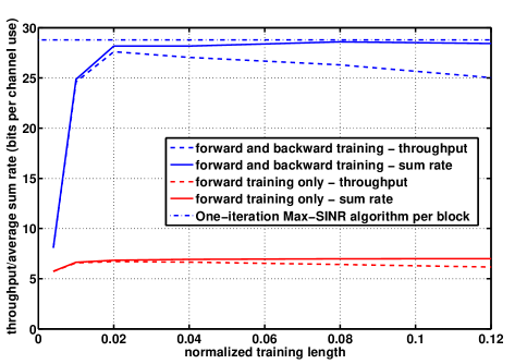
Figure 1: Performance of the bi-directional LS algorithm and the forward training only scheme for constant channels.

Next, to illustrate the effect of varying the number of iterations per coherence block, we consider a network with i.i.d. block fading channels (i,e, $\alpha=0$). Figure 2 shows the sum-rate versus the total training length for a SNR of $20$ dB. Each curve corresponds to a different number of iterations (cycles) per block, where the total amount of training is evenly divided among each iteration. For example, with 128 training symbols and 4 bi-directional iterations, the training alternates between the forward and reverse directions every 16 symbols. As in the previous case, we also show the performance of the Max-SINR algorithm and that of forward training only. Again for this case, the bi-directional training scheme can provide a substantial benefit relative to forward training only. However, the results also indicate that significant training is needed to approach the sum rate possible with perfect channel knowledge. It can also be seen that given a fixed training length there is an optimal number of bi-directional iterations; with too few iterations the transmit beam and receiver filter do not converge to the appropriate fixed point, whereas with too many iterations each segment contains insufficient training symbols to obtain accurate filter estimates. For high SNRs, the tradeoff generally favors more iterations since the number of iterations needed to achieve the optimal fixed point increases with SNR.

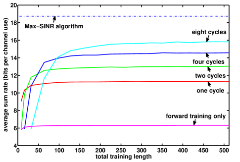
Figure 2: Sum-rate versus training length with bi-directional training and i.i.d. block fading channels. Plots are shown for different numbers of forward-backward iterations (cycles).

Next, to gain insight into the performance of the bi-directional LS algorithm as a function of the SNR, we consider a limiting model in which their is a single iteration per block and the training data per iteration goes to infinity. In this case, each update will be equivalent to the corresponding update in the Max-SINR algorithm. Fig. 3 shows the sum rate yielded by this limiting scheme above versus the SNR for channels with correlated fading corresponding to different choices of $\alpha$. We also show the performance of two schemes in which only two of the three users are allowed to transmit and the two users either update their beams using bi-directional training or forward training only, still assuming an infinite number of training bits per update. First consider the scheme corresponding to three users with $\alpha=1$. In this case the channel is not changing from one iteration to the next and thus the algorithm is the same as the Max-SINR algorithm, which appears to be achieving the optimal high-SNR slope here. When the channel is not constant ($\alpha<1$), the beamformers and receive filters are always mismatched due to the channel fading; this mismatch eventually limits the growth of the sum-rate for the three user schemes as the SNR increases. The two schemes in which only two user transmit have nearly identical performance and both appear to achieve the optimal high-SNR slope for two users with rank 1 codebooks. This is because for a two-user $2\times 2$ MIMO system, it is much easier to orthogonalize the two users and indeed this can be done by only adapting the receive filters, while for a three-user system, both the beamformers and receive filters need to be chosen to achieve alignment. This suggests that for a high enough SNR in a time-varying channel, it may be better to only allow two-users to transmit in this way.

Figure 3: Sum rate performance of the bi-directional LS algorithm with one iteration and infinite training data per block under different channel correlations.

V-B Bi-directional Recursive Least Squares Algorithm

Now we turn to the performance of the bi-directional RLS algorithm. Recall, that this algorithm was motivated for cases where the number of channel uses per block is small and there is significant correlation between blocks. Figures 4 and 5 show the performance of the bi-directional RLS with different choices of $\lambda$ and LS algorithms as a function of the training length in a channels with correlated fading corresponding to $\alpha=0.99$ and $\alpha=0.999$, respectively. Both the sum-rate (solid lines) and the throughput (dashed lines) of each algorithm is shown as well as for forward-training only. For all the algorithms, a single iteration of training is used per block and the SNR is 10db. It can be seen that when the total training length is limited the bi-directional RLS algorithm with an appropriate $\lambda$ gives a higher sum-rate than the LS algorithm, while if training bits are sufficient the LS algorithm gives the high rate. The gains of the bi-directional RLS algorithm are more significant when $\alpha$ is closer to $1$, i.e., the channel is varying more slowly. When we consider the throughput accounting for training overhead, the gains of the bi-directional RLS algorithm diminish, and for $\alpha=0.99$ become insignificant for most ranges of training. Of course this comparison depends on the block-length $L$, which here we assume is given by $L=\frac{1}{1-\alpha}$. In other simulations, we have also observed that the performance benefits of the RLS algorithm are greater at lower SNRs, i.e. when estimation becomes more difficult.

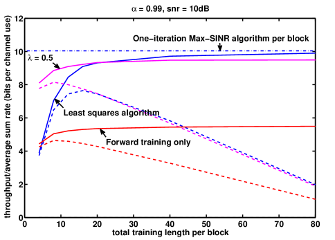
Figure 4: Comparison between the LS algorithm and the RLS algorithm with $\lambda=0.5$ ($\alpha=0.99$).

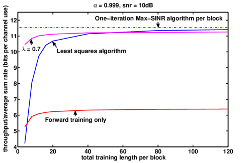
Figure 5: Comparison between the LS algorithm and the RLS algorithm with $\lambda=0.7$ ($\alpha=0.999$).

VI Conclusions

We have presented a distributed algorithm for iteratively adapting beamformers and receive filters in MIMO interference networks without CSI. The algorithm is based on using bi-directional training in a synchronous TDD system. This algorithm approaches the performance of the Max-SINR algorithm with full CSI as the amount of training and the number of training cycles increase. A recursive modification of the algorithm that uses exponentially weighted data from previous blocks was also given and shown to offer better performance when the channels are highly correlated and the training length very small. Here we mainly demonstrated the performance of these algorithms via simulations; analyzing the performance is an interesting direction for future work.

References

- [1] K. S. Gomadam, V. R. Cadambe, and S. A. Jafar, “Approaching the Capacity of Wireless Networks through Distributed Interference Alignment,” in Proc. of IEEE GLOBECOM, Nov./Dec. 2008.
- [2] D. A. Schmidt, C. Shi, R. A. Berry, M. L. Honig, and W. Utschick, “Minimum Mean Squared Error Interference Alignment,” in Proc. of Asilomar Conference on Signals, Systems, and Computers, Nov., 2009.
- [3] C. Shi, D. A. Schmidt, R. A. Berry, M. L. Honig, and W. Utschick, “Distributed Interference Pricing for the MIMO Interference Channel,” in Proc. IEEE International Conference on Communications, June 2009.
- [4] V. R. Cadambe and S. A. Jafar, “Interference Alignment and the Degrees of Freedom for the K User Interference Channel,” IEEE Transactions on Information Theory, vol. 54, no. 8, pp. 3425-3441, Aug. 2008.
- [5] S. W. Peters and R. W. Heath, Jr., “Cooperative Algorithms for MIMO Interference Channels,” submitted to IEEE Transactions on Vehicular Technology, Dec. 2009.
- [6] T. L. Marzetta, “How much training is required for multiuser MIMO?” In Proc. Asilomar Conf. on Signals, Systems, and Computers, pp. 359-363, Pacific Beach, Ca., 2006.
- [7] X. Zhou, T. A. Lamahewa, P. Sadeghi, and S. Durrani, “Two-Way Training: Optimal Power Allocation for Pilot and Data Transmission,” IEEE Trans. on Wireless Communications, Feb. 2010.
- [8] K. S. Gomadam, H. C. Papadopoulos, and C.-E. W. Sundberg, “Techniques for Multi-user MIMO with Two-way Training,” in Proc. IEEE International Conference on Communications, May, 2008.
- [9] R. Osawa, H. Murata, K. Yamamoto, and S. Yoshida, “Performance of Two-Way Channel Estimation Technique for Multi-User Distributed Antenna Systems with Spatial Precoding,” in Proc. Vehicular Technology Conference Fall (VTC 2009-Fall), Sept. 2009.
- [10] C. Steger and A. Sabharwal, “Single-input Two-way SIMO Channel: Diversity-multiplexing Tradeoff with Two-way Training,” IEEE Transactions on Wireless Communications, Dec. 2008.
- [11] L. P. Withers, R. M. Taylor, and D. M. Warme, “Echo-MIMO: A Two-Way Channel Training Method for Matched Cooperative Beamforming,” IEEE Transactions on Signal Processing. Sept. 2008.