Geometric measures of entanglement and the Schmidt decomposition

Abstract

In the standard geometric approach, the entanglement of a pure state is $\sin^{2}\theta$, where $\theta$ is the angle between the entangled state and the closest separable state of products of normalised qubit states. We consider here a generalisation of this notion by considering separable states that consist of products of unnormalised states of different dimension. The distance between the target entangled state and the closest unnormalised product state can be interpreted as a measure of the entanglement of the target state. The components of the closest product state and its norm have an interpretation in terms of, respectively, the eigenvectors and eigenvalues of the reduced density matrices arising in the Schmidt decomposition of the state vector. For several cases where the target state has a large degree of symmetry, we solve the system of equations analytically, and look specifically at the limit where the number of qubits is large.

I Introduction

With recognition of its role as a resource in quantum computing nielsen , the nature of entanglement in quantum systems is a problem of much current interest review1 ; review2 ; review3 . Of particular importance is a quantitative measure of entanglement quantify . Two of the more commonly used measures are the von Neumann entropy, which is based on reduced density matrices review1 , and a geometric measure, which is based on the distance to the nearest product state g1 ; g2 ; g3 ; g4 ; witness . In this paper we introduce a geometric measure of entanglement based on the distance between an unnormalised product state and a target entangled state. The norm of the closest product state can be related to both the distance and angle between the product and target states. This result motivates the interpretation of the distance to the closest product state as a measure of the entanglement of the initial state.

We begin by defining our notation. We consider a system of $q$ qubits. The dimension of the corresponding Hilbert space is $n=2^{q}$. We will decompose the system into a set of subsystems. The subsystems are labelled $A,B,C,\cdots$ They have dimension $u,v,w,\cdots$ such that $n=u\cdot v\cdot w\cdots$. An arbitrary set of basis states of system $A$ is labelled $|i\rangle$, the basis states of $B$ are $|j\rangle$, the basis states of $C$ are $|k\rangle$, etc. Using this notation we write:

$$|A\rangle=\sum_{i=0}^{u-1}a_{i}|i\rangle,~{}~{}|B\rangle=\sum_{j=0}^{v-1}b_{i}|j\rangle,~{}~{}|C\rangle=\sum_{k=0}^{w-1}c_{i}|k\rangle,~{}~{}\dots$$ (1)

We consider an arbitrary normalised entangled pure state and write its wave-function:

$$|\psi\rangle=\sum_{i=0}^{u-1}\sum_{j=0}^{v-1}\sum_{k=0}^{w-1}\cdots\chi_{ijk\cdots}|i\rangle\otimes|j\rangle\otimes|k\rangle\cdots~{},~{}~{}~{}\langle\psi|\psi\rangle=1\,.$$ (2)

In this paper we introduce a new geometric measure of the entanglement of this state. The paper is organised as follows. In section II we introduce our geometric measure of entanglement. In section III we show that, for a given entangled state, a connection can be established between the components and norm of the closest product state, and the basis states and eigenvalues of the Schmidt decomposition of the entangled state. In section IV we study some general symmetries of our measure. In section V we derive some exact solutions for cases where the target state $|\psi\rangle$ has a large degree of symmetry, and in section VI we present our conclusions.

II Optimum Euclidean Distance

In this section we introduce a new geometric measure of entanglement. We look at the distance between the pure entangled state (2) and an arbitrary unnormalised product state. Extremizing this distance allows us to identify the closest product state. The distance between the state $|\psi\rangle$ and this closest product state is our geometric measure of the entanglement of $|\psi\rangle$.

We consider the product state:

$$|\phi\rangle=|A\rangle\otimes|B\rangle\otimes|C\rangle\otimes\ldots=\sum_{i=0}^{u-1}a_{i}|i\rangle\otimes\sum_{j=0}^{v-1}b_{j}|j\rangle\otimes\sum_{k=0}^{w-1}c_{j}|k\rangle\otimes\ldots$$ (3)

The state $|\phi\rangle$ is not assumed to be normalised:

$$\langle\phi|\phi\rangle=N_{A}N_{B}N_{C}\ldots;~{}~{}N_{A}=\langle A|A\rangle=\displaystyle\sum_{i=0}^{u-1}a_{i}^{*}a_{i},~{}~{}N_{B}=\langle B|B\rangle=\displaystyle\sum_{j=0}^{v-1}b_{j}^{*}b_{j},~{}~{}\cdots$$ (4)

The distance between the states $|\psi\rangle$ and $|\phi\rangle$ is:

$$D^{2} =\langle\phi-\psi|\phi-\psi\rangle\,,$$ (5)

$$=1-\langle\phi|\psi\rangle-\langle\psi|\phi\rangle+N_{A}N_{B}N_{C}\ldots$$

$$=\left(\sum_{i=0}^{u-1}\sum_{j=0}^{v-1}\sum_{k=0}^{w-1}\cdots\right)\left(a_{i}^{*}b_{j}^{*}c_{k}^{*}\ldots-\chi_{ijk\cdots}^{*}\right)\left(a_{i}b_{j}c_{k}\ldots-\chi_{ijk\cdots}\right)\,.$$

We extremize this distance with respect to the coordinates of $|A\rangle,|B\rangle,\ldots$

$$\frac{\partial D^{2}}{\partial a_{i}}=0 \Rightarrow a_{i}^{*}N_{B}N_{C}\ldots=\left(\sum_{j=0}^{v-1}\sum_{k=0}^{w-1}\cdots\right)b_{j}c_{k}\ldots\chi_{ijk\ldots}^{*}$$

$$\frac{\partial D^{2}}{\partial b_{j}}=0 \Rightarrow b_{j}^{*}N_{A}N_{C}\ldots=\left(\sum_{i=0}^{u-1}\sum_{k=0}^{w-1}\cdots\right)a_{i}c_{k}\ldots\chi_{ijk\ldots}^{*}$$

$$\frac{\partial D^{2}}{\partial c_{k}}=0 \Rightarrow c_{k}^{*}N_{A}N_{B}\ldots=\left(\sum_{i=0}^{u-1}\sum_{j=0}^{v-1}\cdots\right)a_{i}b_{j}\ldots\chi_{ijk\ldots}^{*}$$ (6)

$$\vdots$$

Rewriting Eq. (6), we have:

$$N_{A}N_{B}N_{C}\ldots=\left(\sum_{i=0}^{u-1}\sum_{j=0}^{v-1}\sum_{k=0}^{w-1}\cdots\right)a_{i}b_{j}c_{k}\ldots\chi_{ijk\ldots}^{*}=\langle\psi|\phi\rangle\,.$$ (7)

In exactly the same way we could extremize the distance in Eq. (5) with respect to the coordinates of $\langle A|,\langle B|,\ldots$ and obtain: $N_{A}N_{B}N_{C}\ldots=\langle\phi|\psi\rangle$. Substituting these results into (5) we find that at the extrema the distance between $|\psi\rangle$ and $|\phi\rangle$ is:

$$D_{C}^{2}=1-N_{A}N_{B}N_{C}\ldots=1-\cos^{2}\theta_{C}\,,$$ (8)

where we have defined the critical angle $\theta_{C}$ as the angle between $|\psi\rangle$ and $|\phi\rangle$ at the extrema:

$$\cos\theta_{C}=\left.\frac{\langle\psi|\phi\rangle}{\sqrt{\langle\phi|\phi\rangle}\sqrt{\langle\psi|\psi\rangle}}\right|_{\rm critical}=\sqrt{N_{A}N_{B}N_{C}\ldots}$$ (9)

In order to demonstrate the consistency of these results, we look at the Cauchy–Schwartz inequality which requires:

$$\langle\phi-\psi|\phi-\psi\rangle\langle\phi|\phi\rangle\geq\left|\langle\phi-\psi|\phi\rangle\right|^{2}\,.$$ (10)

Using (4) and (5) we have:

$$D^{2}\cdot(N_{A}N_{B}N_{C}\cdots)\geq\left|(N_{A}N_{B}N_{C}\cdots)-\langle\psi|\phi\rangle\right|^{2}\,.$$ (11)

Using (7) and (8) we find that at the extrema

$$1-N_{A}N_{B}N_{C}\cdots\geq 0~{}~{}\Rightarrow~{}~{}N_{A}N_{B}N_{C}\cdots\leq 1\,.$$ (12)

This inequality guarantees that the cosine of the critical angle (Eq. (9)) is a real number which satisfies $1>\cos\theta_{C}>-1$, and that the square of the critical distance (Eq. (8)) is real and positive.

We can compare the results in Eqs. (8), (9) with those that would be obtained using a product of normalised states. We use $\langle A|A\rangle=\langle B|B\rangle=\cdots=1$. We take the derivative of $D^{2}$ with respect to $a_{i}$ as before, but now we insert a Lagrange multiplier term of the form $\lambda\langle A|A\rangle$. This approach produces the same critical angle as before (Eq. (9)). The corresponding minimal distance is:

$$D_{N}^{2}=\langle\phi_{N}-\psi|\phi_{N}-\psi\rangle=D^{2}+\left(1-\sqrt{\langle\phi|\phi\rangle}\right)^{2}=2(1-\cos\theta_{C})\,,$$ (13)

which can be compared with the result for unnormalised product states (Eq. (8)).

Figure 1: Geometrical comparison of the entanglement measure using unnormalised ($\vec{\phi}$) and normalised ($\vec{\phi}_{N}$) separable states.

III Connection to the Schmidt decomposition

The equations in (6) which determine the extremal points of the distance to the closest product state are non–linear and must be solved numerically, except in special cases. One of the special cases for which a closed–form solution exists occurs when the $n$–dimensional system is decomposed into two subsystems. We consider a $u$-dimensional subsystem $A$, and a $v$-dimensional subsystem $B$, such that $n=uv$. In this case the equations (6) decouple to yield:

$$a_{i}N_{A}N_{B} = \sum_{i^{\prime}=0}^{u-1}\sum_{j=0}^{v-1}\chi_{ij}\chi_{i^{\prime}j}^{*}a_{i^{\prime}}\,,$$

$$b_{j}N_{A}N_{B} = \sum_{j^{\prime}=0}^{v-1}\sum_{i=0}^{u-1}\chi_{ij}\chi_{ij^{\prime}}^{*}b_{j^{\prime}}\,.$$ (14)

Each of these equations can be solved for the product $N_{A}N_{B}$ and give, respectively:

$${\rm det}\left|N_{A}N_{B}\delta_{ii^{\prime}}-\sum_{j=0}^{v-1}\chi_{ij}\chi_{i^{\prime}j}^{*}\right| = 0\,,$$

$${\rm det}\left|N_{A}N_{B}\delta_{jj^{\prime}}-\sum_{i=0}^{u-1}\chi_{ij}\chi_{ij^{\prime}}^{*}\right| = 0\,.$$ (15)

These solutions can be related to the eigenvalues of the reduced density matrix. We consider the $n$-dimensional state in Eq. (2) and write its wave-function and density matrix in the computational basis:

$$|\psi\rangle=\sum_{z=0}^{n-1}\chi_{z}|z\rangle\,,~{}~{}\rho=\sum_{z=0}^{n-1}\sum_{z^{\prime}=0}^{n-1}\chi_{z}\chi^{*}_{z^{\prime}}|z\rangle\langle z|\,.$$ (16)

Decomposing the system into a $u$-dimensional subsystem $A$ and a $v$-dimensional subsystem $B$, we obtain:

$$|\psi\rangle=\sum_{i=0}^{u-1}\sum_{j=0}^{v-1}\chi_{ij}|i\rangle\otimes|j\rangle\,,~{}~{}~{}\rho=\sum_{i=0}^{u-1}\sum_{i^{\prime}=0}^{u-1}\sum_{j=0}^{v-1}\sum_{j^{\prime}=0}^{v-1}\chi_{ij}\chi^{*}_{i^{\prime}j^{\prime}}|i\rangle\langle i^{\prime}|\otimes|j\rangle\langle j^{\prime}|\,.$$ (17)

Next we calculate the reduced density matrices. The reduced density matrix $\rho_{A}$ is obtained by tracing over the subsystem $B$, and the reduced density matrix $\rho_{B}$ is obtained by tracing over the subsystem $A$. The definitions are:

$${\rm Tr}_{A}(\rho) = \sum_{t=0}^{u-1}\left(\langle t|\otimes\mathds{1}_{B}\right)\rho\left(|t\rangle\otimes\mathds{1}_{B}\right)\,,$$

$${\rm Tr}_{B}(\rho) = \sum_{t=0}^{v-1}\left(\mathds{1}_{A}\otimes\langle t|\right)\rho\left(\mathds{1}_{A}\otimes|t\rangle\right)\,,$$ (18)

where $\mathds{1}_{A}$ and $\mathds{1}_{B}$ are the identity matrices in the subspaces of $A$ and $B$, respectively. We obtain:

$$\rho_{A}={\rm Tr}_{B}(\rho) = \sum_{t=0}^{v-1}\sum_{i=0}^{u-1}\sum_{i^{\prime}=0}^{u-1}\sum_{j=0}^{v-1}\sum_{j^{\prime}=0}^{v-1}\chi_{ij}\chi_{i^{\prime}j^{\prime}}^{*}\langle t|j\rangle\langle j^{\prime}|t\rangle|i\rangle\langle i^{\prime}|=\sum_{j=0}^{v-1}\sum_{i=0}^{u-1}\sum_{i^{\prime}=0}^{u-1}\chi_{ij}\chi_{i^{\prime}j}^{*}|i\rangle\langle i^{\prime}|\,,$$ (19)

or, in terms of components:

$$\left(\rho_{A}\right)_{ii^{\prime}}=\sum_{j=0}^{v-1}\chi_{ij}\chi_{i^{\prime}j}^{*}\,.$$ (20)

Similarly, the reduced density matrix $\rho_{B}={\rm Tr}_{A}(\rho)$ is obtained by tracing over the subsystem $A$ and can be written:

$$\left(\rho_{B}\right)_{jj^{\prime}}=\sum_{i=0}^{u-1}\chi_{ij}\chi_{ij^{\prime}}^{*}\,.$$ (21)

Using Eqs. (20) and (21) we can rewrite the extremal conditions of Eqs. (14) in the form:

$$\sum_{i=0}^{u-1}\left(\rho_{A}\right)_{ii^{\prime}}a_{i^{\prime}} = N_{A}N_{B}a_{i}\,,$$

$$\sum_{j=0}^{v-1}\left(\rho_{B}\right)_{jj^{\prime}}b_{j^{\prime}} = N_{A}N_{B}b_{j}\,.$$ (22)

Equation (22) shows that $N_{A}N_{B}$ are the eigenvalues corresponding to the eigenvectors $a_{i}$ and $b_{j}$ of the reduced density matrices $\rho_{A}$ and $\rho_{B}$.

This result can be interpreted in terms of the Schmidt decomposition as follows nielsen ; s1 ; s2 ; s3 ; s4 ; s5 . Let us write the extrema conditions of Eq.(6) as

$${\widehat{a}_{i}}\sigma = \sum_{j=0}^{v-1}\chi_{ij}\,{\widehat{b}_{j}}^{*}$$

$${\widehat{b}_{j}}\sigma = \sum_{i=0}^{u-1}{\widehat{a}_{i}}^{*}\,\chi_{ij}$$ (23)

where ${\widehat{a}_{i}}=a_{i}/\sqrt{N_{A}}$ and ${\widehat{b}_{j}}=b_{j}/\sqrt{N_{B}}$ are, respectively, the left–singular and right–singular vectors corresponding to the singular values $\sigma=\sqrt{N_{A}N_{B}}$ of the matrix $\chi$. The singular value decomposition of the matrix $\chi$ can then be written as

$$\chi=A\,\Sigma\,B^{\dagger}$$ (24)

where the columns of the (unitary) matrices $A$ and $B$ are, respectively, the vectors ${\widehat{a}_{i}}$ and ${\widehat{b}_{j}}$, and $\Sigma$ is a diagonal matrix whose elements are the singular values $\sigma$. This can be used to rewrite the state $|\psi\rangle$ in (17) in terms of the Schmidt decomposition involving a single summation:

$$|\psi\rangle=\sum_{k=0}^{{\rm min}(u-1,v-1)}\sqrt{p_{k}}\ |\alpha_{k}\rangle\otimes|\beta_{k}\rangle\,,$$ (25)

where the Schmidt coefficients $p_{k}$, which are identified with the singular values $\sigma$, satisfy $\sum_{k}p_{k}=1$, and the states $|\alpha_{k}\rangle$ and $|\beta_{k}\rangle$ are identified with, respectively, the left–singular and right–singular vectors ${\widehat{a}_{i}}$ and ${\widehat{b}_{j}}$. Calculating the corresponding reduced density matrices using (18) we obtain:

$$\rho_{A} = {\rm Tr}_{B}(\rho)=\sum_{k}p_{k}\ |\alpha_{k}\rangle\langle\alpha_{k}|\,,$$

$$\rho_{B} = {\rm Tr}_{A}(\rho)=\sum_{k}p_{k}\ |\beta_{k}\rangle\langle\beta_{k}|\,,$$ (26)

from which one can see that $|\alpha_{k}\rangle$ are the eigenvectors of $\rho_{A}={\rm Tr}_{B}(\rho)$ and $|\beta_{k}\rangle$ are the eigenvectors of $\rho_{B}={\rm Tr}_{A}(\rho)$ with corresponding eigenvalues $p_{k}$.

We remark that the Schmidt decomposition gives rise to several other measurements of entanglement. The reduced density matrices $\rho_{A}$ and $\rho_{B}$ in (III) have the same non-zero eigenvalues and, for a product state, only one non–zero eigenvalue is present. As a result, for a non-product state, the eigenvalues of the reduced density matrix can be used to quantify the degree of entanglement. One commonly used measure of entanglement is the von Neumann entropy:

$$S=-{\rm Tr}\left(\rho_{A}\ln\rho_{A}\right)=-{\rm Tr}\left(\rho_{B}\ln\rho_{B}\right)=-\sum_{k}p_{k}\log_{2}p_{k}\,.$$ (27)

It is interesting to consider the particular case that the $n$–dimensional space is split into the product of a single qubit space and another space of dimension $u=n/2$. In this case, one of the equations in (15) will become a quadratic equation for the product $N_{A}N_{B}$ with solutions:

$$N_{A}N_{B}\equiv\mu_{\pm}=\frac{1}{2}\left[1\pm\sqrt{1-4C}\right],\qquad\qquad C=\sum_{j=1}^{u-1}\sum_{k=0}^{j-1}\left|\chi_{0j}\chi_{1k}-\chi_{1j}\chi_{0k}\right|^{2}\,.$$ (28)

The Schmidt decomposition (Eq. (25)) becomes:

$$|\psi\rangle=\sqrt{\mu_{+}}\ |\alpha_{+}\rangle\otimes|\beta_{+}\rangle+\sqrt{\mu_{-}}\ |\alpha_{-}\rangle\otimes|\beta_{-}\rangle\,.$$ (29)

Using Eq. (9) we can relate the eigenvalues $N_{A}N_{B}=\mu_{\pm}$ to the cosine of the angle between $|\psi\rangle$ and the closest product state $|\phi\rangle$. Since $\mu_{+}$ is the larger of the two eigenvalues we write $\cos\theta_{\rm max}\equiv\mu_{+}$ and Eq. (29) becomes:

$$|\psi\rangle=\cos\theta_{\rm max}\ |\alpha_{+}\rangle\otimes|\beta_{+}\rangle+\sin\theta_{\rm max}\ |\alpha_{-}\rangle\otimes|\beta_{-}\rangle\,.$$ (30)

If $|\psi\rangle$ was a product state, the reduced density matrix would have only one non-zero eigenvalue and we would have $\mu_{-}=\sin^{2}\theta_{\rm max}=0$. This result is consistent with our geometric approach: from Eq. (8), $\sin^{2}\theta_{\rm max}=0$ corresponds to a zero minimal distance between the state $|\psi\rangle$ and the nearest product state, which means that $|\psi\rangle$ is itself a product state.

The Schmidt decomposition can also be applied to multipartite pure states s4 . One starts with a state $|\psi\rangle$ and decomposes it into two subsystems: a single qubit system $A$, and a subsystem ($BC\ldots Z$) containing all other qubits. Using a Schmidt decomposition we can write:

$$|\psi\rangle=\sum_{i_{a}}\sqrt{p_{i_{a}}^{A}}|\psi_{i_{a}}^{A}\rangle\otimes|\psi_{i_{a}}^{BC\ldots Z}\rangle\,.$$ (31)

One then decomposes $|\psi_{i_{a}}^{BC\ldots Z}\rangle$ into two subsystems: another single qubit system $B$, and a subsystem ($CD\ldots Z$) containing all other qubits. Using a Schmidt decomposition we can write:

$$|\psi_{i_{a}}^{BC\ldots Z}\rangle=\sum_{i_{b}}\sqrt{p_{i_{a};i_{b}}^{B}}|\psi_{i_{a};i_{b}}^{B}\rangle\otimes|\psi_{i_{a};i_{b}}^{CD\ldots Z}\rangle\,.$$ (32)

This process is continued until the last two qubit spaces $Y$ and $Z$ are reached, with the result:

$$|\psi\rangle=\sum_{i_{a}i_{b}\ldots i_{y}}\sqrt{p_{i_{a}}^{A}p_{i_{a};i_{b}}^{B}\cdots p_{i_{a}i_{b}\ldots i_{x};i_{y}}^{Y}}|\psi_{i_{a}}^{A}\rangle\otimes|\psi_{i_{a};i_{b}}^{B}\rangle\otimes\cdots\otimes|\psi_{i_{a}i_{b}\ldots i_{x};i_{y}}^{Y}\rangle\otimes|\psi_{i_{a}i_{b}\ldots i_{x};i_{y}}^{Z}\rangle\,.$$ (33)

Now we consider the geometric interpretation of this result. Consider the distance between $|\psi\rangle$ and a state $|\phi^{A;BC\ldots Z}\rangle=|\phi^{A}\rangle\otimes|\phi^{BC\ldots Z}\rangle$, where $|\phi^{A}\rangle$ is a single qubit state and $|\phi^{BC\ldots Z}\rangle$ is the state of the remaining qubits. This distance is:

$$D_{A;BC\ldots Z}^{2}=\big{\langle}\psi-\left[\phi^{A}\otimes\phi^{BC\ldots Z}\right]\big{|}\psi-\left[\phi^{A}\otimes\phi^{BC\ldots Z}\right]\big{\rangle}\,.$$ (34)

Finding the extremal points of this distance will result in a system of (linear) equations, as in Eq. (15), which determine the components of the state $|\phi^{A;BC\ldots Z}\rangle$. There is a direct correspondence between the coefficients of the closest product state and the basis states of the Schmidt decomposition (Eq. (31)), and the norm of the closest product state is related to the corresponding Schmidt coefficients.

We can then consider the distance between the state $|\phi^{BC\ldots Z}\rangle$ and a state $|\phi^{B;CD\ldots Z}\rangle=|\phi^{B}\rangle\otimes|\phi^{CD\ldots Z}\rangle$:

$$D_{B;CD\ldots Z}^{2}=\big{\langle}\phi^{BC\ldots Z}-\left[\phi^{B}\otimes\phi^{CD\ldots Z}\right]\big{|}\phi^{BC\ldots Z}-\left[\phi^{B}\otimes\phi^{CD\ldots Z}\right]\big{\rangle}\,,$$ (35)

where $|\phi^{B}\rangle$ is a single qubit state and $|\phi^{CD\ldots Z}\rangle$ is the state of the remaining qubits. Extremizing this distance will again result in a system of linear equations determining the components of the state $|\phi^{B;CD\ldots Z}\rangle$. Once again, there is a direct correspondence between the coefficients of the closest product state and the basis states of the Schmidt decomposition (Eq. (32)), and the norm of the closest product state is related to the corresponding Schmidt coefficients.

This process may be continued until the last two qubit states $|\phi^{Y}\rangle$ and $|\phi^{Z}\rangle$ are reached. In analogy with Eq. (9), we can define the cosine of the critical angle $\theta_{C}$:

$$\cos\theta_{C}=\left.\frac{\langle\psi|\phi\rangle}{\sqrt{\langle\phi|\phi\rangle}\sqrt{\langle\psi|\psi\rangle}}\right|_{\rm critical}\qquad\qquad\ldots\quad|\phi\rangle=|\phi^{A}\rangle\otimes|\phi^{B}\rangle\otimes\cdots|\phi^{Z}\rangle\,.$$ (36)

The quantity $\sin^{2}\theta_{C}=1-\cos^{2}\theta_{C}$ is a measure of the entanglement of the original multipartite state.

The advantage of this procedure is that it involves solving a series of linear equations, as compared to the approach of Section II which produces the non–linear equations of Eq. (6). The disadvantage is that the result depends on the order that the series of decompositions is made: the sequence $ABC\ldots YZ$ described above will differ from the sequence $BC\ldots ZA$. In Ref. s4 , the entanglement is given by the minimal value obtained by looking at all permutations of the possible orders of the decompositions.

IV Symmetries

The equation that gives the distance between the target entangled state and the nearest product state (Eq. (8)) is invariant under certain transformations of the parameters $\{a_{i},b_{i},\ldots\}$. In order to see these symmetries explicitly we can reparameterize each set of coefficients. For the coefficients $a_{i}$ we write:

$$a_{i} = A_{i}e^{i\alpha_{i}^{a}}\,.$$ (37)

with similar equations for the coefficients $\{b_{i},c_{i},\ldots\}$. Using generalised spherical coordinates in $n$ dimensions we can rewrite the set of real variables $A_{i}$ in terms of a magnitude $A$ and ($n-1$) angles $\theta_{i}$:

$$\left(\begin{array}[]{c}A_{1}\\ A_{2}\\ A_{3}\\ \vdots\\ A_{k}\\ \vdots\\ A_{n-1}\\ A_{n}\end{array}\right)=A\left(\begin{array}[]{c}\cos\theta_{1}\\ \sin\theta_{1}\cos\theta_{2}\\ \sin\theta_{1}\sin\theta_{2}\cos\theta_{3}\\ \vdots\\ \left(\Pi_{i=1}^{k-1}\sin\theta_{i}\right)\cos\theta_{k}\\ \vdots\\ \sin\theta_{1}\cdots\sin\theta_{n-2}\cos\theta_{n-1}\\ \sin\theta_{1}\cdots\sin\theta_{n-2}\sin\theta_{n-1}\end{array}\right)\equiv Af_{i}(\theta^{a})\,.$$ (38)

We can also parameterise the phase angles $\alpha_{i}^{a}$ as:

$$e^{i\alpha_{i}}\left(\begin{array}[]{c}e^{i\alpha_{1}}\\ e^{i\alpha_{2}}\\ \vdots\\ e^{i\alpha_{n}}\end{array}\right)=e^{i\alpha_{1}}\left(\begin{array}[]{c}1\\ e^{i(\alpha_{2}-\alpha_{1})}\\ \vdots\\ e^{i(\alpha_{n}-\alpha_{1})}\end{array}\right)\equiv e^{i\alpha_{1}}\left(\begin{array}[]{c}1\\ e^{i\beta_{2}}\\ \vdots\\ e^{i\beta_{n}}\end{array}\right)\equiv e^{i\alpha_{1}}e^{i\beta_{i}}\,,$$ (39)

where $\beta_{1}\equiv 0$. Using this notation we write:

$$a_{i} = Ae^{i\alpha_{1}^{a}}f_{i}(\theta^{a})e^{i\beta_{i}^{a}}$$

$$b_{i} = Be^{i\alpha_{1}^{b}}f_{i}(\theta^{b})e^{i\beta_{i}^{b}}$$ (40)

$$\vdots$$

We can use this parameterisation to rewrite the distance function (8). We make the definitions:

$$\langle\phi|\phi\rangle \equiv N^{2}\,,$$

$$|\phi\rangle \equiv N|\hat{\phi}\rangle\,,~{}~{}~{}\langle\hat{\phi}|\hat{\phi}\rangle=1\,.$$ (41)

Note that the first line in (IV) gives:

$$\langle\phi|\phi\rangle=A^{2}B^{2}C^{2}\cdots=N_{A}N_{B}N_{c}\cdots=N^{2}\,.$$ (42)

Using these definitions the distance in Eq. (5) becomes:

$$D^{2}=N^{2}-N\left[\langle\psi|{\hat{\phi}}\rangle+\langle{\hat{\phi}}|\psi\rangle\right]+1\,.$$ (43)

Extremizing we obtain:

$$\frac{\partial D^{2}}{\partial N}=0 \Rightarrow 2N-\left[\langle\psi|{\hat{\phi}}\rangle+\langle{\hat{\phi}}|\psi\rangle\right]=0\,,$$ (44)

$$\Rightarrow N={\rm Re}\left[\langle\psi|{\hat{\phi}}\rangle\right]\,,$$

which means that at the extrema:

$$D_{C}^{2}=N^{2}-N(2N)+1=1-N^{2}\,.$$ (45)

We note that Eqs. (42) and (45) are consistent with (8).

To make this result more clear, we can look explicitly at the dependence of the distance function on the overall phase of the coefficients of the product state. We define the overall phase angle $\delta=\alpha_{1}^{a}+\alpha_{1}^{b}+\ldots$ and obtain:

$$\langle\phi|\psi\rangle = N\langle{\hat{\phi}}|\psi\rangle=Ne^{-i\delta}\sum_{i=1}^{u}\sum_{j=1}^{v}\cdots f_{i}(\theta^{a})e^{-i\beta_{i}^{a}}f_{j}(\theta^{b})e^{-i\beta_{j}^{b}}\ldots\chi_{ij\cdots}\,,$$

$$\langle\psi|\phi\rangle = N\langle\psi|{\hat{\phi}}\rangle=Ne^{i\delta}\sum_{i=1}^{u}\sum_{j=1}^{v}\cdots f_{i}(\theta^{a})e^{i\beta_{i}^{a}}f_{j}(\theta^{b})e^{i\beta_{j}^{b}}\ldots\chi_{ij\cdots}^{*}\,,$$ (46)

which gives:

$$\frac{\partial}{\partial\delta}\langle\psi|\phi\rangle = N\frac{\partial}{\partial\delta}\langle\psi|{\hat{\phi}}\rangle=iN\langle\psi|{\hat{\phi}}\rangle\,,$$

$$\frac{\partial}{\partial\delta}\langle\phi|\psi\rangle = N\frac{\partial}{\partial\delta}\langle{\hat{\phi}}|\psi\rangle=-iN\langle\psi|{\hat{\phi}}\rangle\,.$$ (47)

From Eq. (43) we have:

$$\frac{\partial D^{2}}{\partial\delta}=-N\frac{\partial}{\partial\delta}\left[\langle\psi|{\hat{\phi}}\rangle+\langle{\hat{\phi}}|\psi\rangle\right]=-iN\left[\langle\psi|{\hat{\phi}}\rangle-\langle{\hat{\phi}}|\psi\rangle\right]=2N{\rm Im}\langle\psi|{\hat{\phi}}\rangle\,,$$ (48)

which means that at the extrema, ${\rm Im}\langle\psi|{\hat{\phi}}\rangle=0$. From Eq. (44) we obtain that at the extrema:

$$N=\langle\psi|{\hat{\phi}}\rangle=\langle{\hat{\phi}}|\psi\rangle\,.$$ (49)

This means that the critical angle defined by:

$$\cos{\hat{\theta}_{C}}=\left.\frac{\langle\psi|{\hat{\phi}}\rangle}{\sqrt{\langle{\hat{\phi}}|{\hat{\phi}}\rangle}\sqrt{\langle\psi|\psi\rangle}}\right|_{\rm critical}=N\,,$$ (50)

is the same critical angle as in Eq. (9).

V Exact Solutions

In this section we look at some states with a large degree of symmetry for which the equations (6) can be solved exactly. We consider a system of $q$ qubits and divide the Hilbert space of dimension $n=2^{q}$ into $q$ spaces, each of dimension 2. Using the notation of section I we have $n=u\cdot v\cdot w\cdots$ with $u=v=w=\cdots=2$. The basis states in each single qubit system are:

$$|0\rangle=\left(\begin{array}[]{c}1\\ 0\end{array}\right)\,,~{}~{}|1\rangle=\left(\begin{array}[]{c}0\\ 1\end{array}\right)\,.$$ (55)

The product state in Eq. (3) becomes:

$$|\phi\rangle =(a_{0}|0\rangle+a_{1}|1\rangle)(b_{0}|0\rangle+b_{1}|1\rangle)(c_{0}|0\rangle+c_{1}|1\rangle)\cdots$$ (56)

$$=(a_{0}b_{0}c_{0}\cdots)|0,0,0,\cdots\rangle+(a_{0}b_{0}c_{1}\cdots)|0,0,1,\cdots\rangle+(a_{0}b_{1}c_{1}\cdots)|0,1,1,\cdots\rangle+\cdots$$

We look for a solution of the form:

$$a_{0} = b_{0}=\cdots=\alpha_{0}\,,$$

$$a_{1} = b_{1}=\cdots=\alpha_{1}\,,$$ (57)

which means $N_{A}=N_{B}=\cdots\equiv N$.

Case 1

Consider:

$$|\psi\rangle=\sqrt{p}\,|0\,0\,\ldots 0\rangle+\sqrt{1-p}\,|1\,1\,\ldots 1\rangle\,.$$ (58)

The only two non–zero components of $\psi_{ijk\cdots}$ are:

$$\psi_{00\cdots 0} = \sqrt{p}\,,$$

$$\psi_{11\cdots 1} = \sqrt{1-p}\,,$$ (59)

and Eq. (6) becomes:

$$a_{0}N_{B}N_{C}\cdots = \sqrt{p}\,b_{0}c_{0}\cdots$$

$$a_{1}N_{B}N_{C}\cdots = \sqrt{1-p}\,b_{1}c_{1}\cdots$$ (60)

Using Eq. (V), Eq. (60) becomes:

$$\alpha_{0}N^{q-1} = \sqrt{p}\,\alpha_{0}^{q-1}\,,$$

$$\alpha_{1}N^{q-1} = \sqrt{1-p}\,\alpha_{1}^{q-1}\,.$$ (61)

Solving this set of equations we obtain:

$$\alpha_{1}^{2} =\frac{N^{2(q-1)/(q-2)}}{(1-p)^{1/(q-2)}}\,,$$

$$\alpha_{0}^{2} =\frac{(1-p)^{1/(q-2)}}{p^{1/(q-2)}}\alpha_{1}^{2}\,,$$ (62)

which gives:

$$N=\alpha_{0}^{2}+\alpha_{1}^{2} = \frac{N^{2(q-1)/(q-2)}}{(1-p)^{1/(q-2)}}\left[1+\frac{(1-p)^{1/(q-2)}}{p^{1/(q-2)}}\right]\,.$$ (63)

Rearranging we obtain:

$$N^{q}=\frac{p(1-p)}{\left[p^{1/(q-2)}+(1-p)^{1/(q-2)}\right]^{q-2}}\,.$$ (64)

We can look at the large $q$ limit. Defining $A=\left[p^{1/(q-2)}+(1-p)^{1/(q-2)}\right]^{q-2}$ we have,

$$\log A = (q-2)\log\left[p^{1/(q-2)}+(1-p)^{1/(q-2)}\right]\,,$$ (65)

$$= (q-2)\log(p^{1/(q-2)})+(q-2)\log\left[1+\left(\frac{1-p}{p}\right)^{1/(q-2)}\right]\,,$$

$$\approx \log p+(q-2)\log 2+\frac{1}{2}\log\left(\frac{1-p}{p}\right)\,,$$

$$= (q-2)\log 2+\frac{1}{2}\log\left[p(1-p)\right]\,,$$

$$= \log\left[2^{q-2}\sqrt{p(1-p)}\right]\,,$$

which gives

$$N^{q}\approx\frac{\sqrt{p(1-p)}}{2^{q-2}}\,.$$ (66)

Case 2

Consider:

$$|\psi\rangle=\left[\,|1\,0\,\ldots 0\rangle+\,|0\,1\,\ldots 0\rangle+\ldots+|0\,0\,\ldots\,1\rangle\right]/\sqrt{q}\,.$$ (67)

The only non–zero coefficients $\psi_{ijk\cdots}$ are:

$$\psi_{100\cdots 0}=\psi_{010\cdots 0}=\psi_{001\cdots 0}=\cdots=\psi_{000\cdots 1}=\frac{1}{\sqrt{q}}\,,$$ (68)

and Eq. (6) becomes:

$$a_{0}N_{B}N_{C}\cdots = \frac{1}{\sqrt{q}}\left[b_{1}c_{0}d_{0}\cdots+b_{0}c_{1}d_{0}\cdots+b_{0}c_{0}d_{1}\cdots+\ldots\right]$$

$$a_{1}N_{B}N_{C}\cdots = \frac{1}{\sqrt{q}}\,b_{0}c_{0}d_{0}\cdots$$ (69)

Using Eq. (V), Eq. (69) becomes:

$$\alpha_{0}N^{q-1} = \psi\,\alpha_{1}\alpha_{0}^{q-2}(q-1)\,,$$

$$\alpha_{1}N^{q-1} = \psi\,\alpha_{0}^{q-1}\,.$$ (70)

Solving the set of equations in (70) we obtain:

$$\alpha_{1}^{q-2} =\frac{\sqrt{q}N^{q-1}}{(q-1)^{(q-1)/2}}\,,$$

$$\alpha_{0}^{2} =\alpha_{1}^{2}(q-1)\,,$$ (71)

which gives:

$$N=\alpha_{0}^{2}+\alpha_{1}^{2}=\frac{N^{2(q-1)/(q-2)}}{\left(1-\frac{1}{q}\right)^{(q-1)/(q-2)}}\,.$$ (72)

Rearranging we obtain:

$$N^{q}=\left(1-\frac{1}{q}\right)^{q-1}\,.$$ (73)

Case 3

Consider:

$$|\psi\rangle=\left[\,|1\,1\,0\,0\,\ldots 0\rangle+\,|0\,1\,1\,0\,\ldots 0\rangle+\,|0\,0\,1\,1\,\ldots 0\rangle+\ldots+|0\,0\,\ldots\,1\,1\rangle+|1\,0\,\ldots\,0\,1\rangle\right]/\sqrt{q}\,.$$ (74)

The only non–zero coefficients $\psi_{ijk\cdots}$ are:

$$\psi_{11000\cdots 0}=\psi_{01100\cdots 0}=\psi_{00110\cdots 0}=\psi_{00011\cdots 0}=\cdots=\psi_{00000\cdots 11}=\psi_{10000\cdots 01}=\frac{1}{\sqrt{q}}\,.$$ (75)

Using Eq. (V), Eq. (6) gives:

$$N^{q-1} = 2\alpha_{1}^{q-2}\sqrt{q}\,,$$

$$N^{q-1} = \sqrt{q}\alpha_{0}^{2}\alpha_{1}^{q-4}-\frac{2}{\sqrt{q}}\alpha_{0}^{2}\alpha_{1}^{q-4}\,.$$ (76)

Solving the equations in (76) we obtain:

$$\frac{\alpha_{0}}{\alpha_{1}} =\frac{\sqrt{2}}{\sqrt{q-2}}\,,$$

$$\alpha_{1} =\frac{1}{2^{2-q}}\frac{1}{q^{2(q-2)}}N^{(q-1)/(q-2)}\,,$$ (77)

which gives:

$$N=\alpha_{0}^{2}+\alpha_{1}^{2}=\frac{1}{Q-2}2^{1/(2(2-q))}q^{1+1/(q-2)}N^{2(q-1)/(q-2)}\,.$$ (78)

Rearranging we extract:

$$N^{q}=4(q-2)^{q-2}q^{1-q}\,.$$ (79)

Case 4

Consider the case where $|\psi\rangle$ has $q$ qubits consisting of all possible combinations of $p$ entries of “1” and $q-p$ entries of “0”. The normalisation is:

$$\psi^{-1}\equiv\sqrt{{q\choose p}}=\sqrt{\frac{q!}{p!(q-p)!}}$$ (80)

Using Eq. (V), Eq. (6) becomes:

$$\alpha_{0}N^{q-1} = \psi\,\alpha_{1}^{p}\alpha_{0}^{q-p-1}{q-1\choose p}\,,$$

$$\alpha_{1}N^{q-1} = \psi\,\alpha_{1}^{p-1}\alpha_{0}^{q-p}{q-1\choose p-1}\,.$$ (81)

Solving the set of equations in (81) we obtain:

$$\alpha_{1}^{q-2} =\frac{N^{q-1}}{\psi\left(\frac{q}{p}-1\right)^{(q-p)/2}{q-1\choose p-1}}\,,$$

$$\alpha_{0}^{2} =\alpha_{1}^{2}\left(\frac{q}{p}-1\right)\,,$$ (82)

which gives:

$$N=\alpha_{0}^{2}+\alpha_{1}^{2}=\left(\frac{q}{p}\right)^{(p-1)/(q-2)}\frac{N^{2(q-1)/(q-2)}}{\left(1-\frac{p}{q}\right)^{(q-p)/(q-2)}\left[{q-1\choose p-1}\right]^{1/(q-2)}}\,.$$ (83)

Rearranging we obtain:

$$N^{q}=\left(\frac{p}{q}\right)^{p-1}\left(1-\frac{p}{q}\right)^{q-p}{q-1\choose p-1}\,.$$ (84)

In the limit $q\gg p$ limit, we can approximate:

$${q-1\choose p-1}=\frac{(q-1)!}{(p-1)!(q-p)!}\approx\frac{1}{(p-1)!}q^{p-1}+{\cal{O}}\left(q^{p-2}\right)\,,$$

$$\left(1-\frac{p}{q}\right)^{q-p}\approx\exp(-p)\,,$$ (85)

which leads to:

$$N^{q}\approx\frac{p^{p-1}\exp(-p)}{(p-1)!}+{\cal O}\left(\frac{1}{q}\right)\,.$$ (86)

V.1 Results

We show below a graph of our results for the entanglement measure as a function of the number of qubits for the four cases solved in this section.

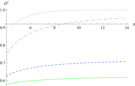
Figure 2: The entanglement as a function of $q$ from Eq. (8) and Eqs. (66) - dotted/red, (73) - solid/green, (79) - dashed/blue and (86) - dot-dashed/magenta.

VI Conclusions

We have considered a generalisation of the usual geometric measure of entanglement of pure states using the distance to the nearest unnormalised product state. This definition does not lead to any computational advantages, since the set of equations that determine the measure are still non–linear in general. However, our definition does provide an interpretation of the standard entanglement measure as the distance to the closest product state. We have also found a relationship between the norm and components of the closest separable state, and the coefficients and basis states of the Schmidt decomposition of the state $|\psi\rangle$. For several cases where the target state has a large degree of symmetry, we have solved the system of non–linear equations analytically, and looked specifically at the limit where the number of qubits is large. These results indicate that our new definition of entanglement, while similar to other definitions that can be found in the literature, is worthy of further study.

References

• (1) M. Nielsen and I. Chuang, Quantum Computation and Quantum Information (Cambridge University Press, 2000).
• (2) Ryszard Horodecki, Pawel Horodecki, Michal Horodecki, and Karol Horodecki, : Rev. Mod. Phys. Vol. 81, No. 2, pp. 865-942 (2009); arXiv:quant-ph/0702225.
• (3) Martin B. Plenio and Shashank Virmani, Quant. Inf. Comp. 7, 1 (2007).
• (4) Karol Zyczkowski and Ingemar Bengtsson, arXiv:quant-ph/0606228v1.
• (5) V. Vedral, M. B. Plenio, M. A. Rippin, and P. L. Knight, Phys. Rev. Lett. 78, 2275 (1997).
• (6) A. Shimony, Ann. N. Y. Acad. Sci. 755, 675 (1995).
• (7) H. Barnum and N. Linden, J. Phys. A34, 6787 (2001).
• (8) Tzu-Chieh Wei and Paul M. Goldbart, Phys. Rev. A68, 042307 (2003).
• (9) Ya Cao and An Min Wang, arXiv:quant-ph/0701099v2.
• (10) Tzu-Chieh Wei and Paul M. Goldbart, arXiv:quant-ph/0303079v1
• (11) Tsubasa Ichikawa, Izumi Tsutsui, and Taksu Cheon, J. Phys. A. 41 (2008) 135303 (29p); arXiv:quant-ph/0702167.
• (12) Jon Magne Leinaas, Jan Myrheim, and Eirik Ovrum, arXiv:quant-ph/0605079.
• (13) A. Yu. Bogdanov, Yu. I. Bogdanov, and K. A. Valiev, arXiv:quant-ph/0512062.
• (14) M. Hossein Partovi, Phys. Rev. Lett. 92, 077904 (2004).
• (15) Ashish V. Thapliyal, Phys. Rev. A59, 3336 (1999).