The Deep Swire Field. IV. First properties of the sub–mJy galaxy population:
redshift distribution, AGN activity and star formation.

Abstract

We present a study of a 20cm selected sample in the Deep SWIRE VLA Field, reaching a 5–$\sigma$ limiting flux density at the image center of $S_{1.4GHz}\sim 13.5\mu$Jy. In a $0.6\times 0.6$ square degrees field, we are able to assign an optical/IR counterpart to 97% of the radio sources. Up to 11 passbands from the NUV to 4.5$\mu$m are then used to sample the spectral energy distribution (SED) of these counterparts in order to investigate the nature of the host galaxies. By means of an SED template library and stellar population synthesis models we estimate photometric redshifts, stellar masses, and stellar population properties, dividing the sample in three sub–classes of quiescent, intermediate and star–forming galaxies. We focus on the radio sample in the redshift range $0.3<z<1.3$ where we estimate to have a redshift completeness higher than 90%, and study the properties and redshift evolution of these sub–populations. We find that, as expected, the relative contributions of AGN and star–forming galaxies to the $\mu$Jy population depend on the flux density limit of the sample. At all flux levels a significant population of “green–valley” galaxies is observed. While the actual nature of these sources is not definitely understood, the results of this work may suggest that a significant fraction of faint radio sources might be composite (and possibly transition) objects, thus a simple “AGN vs star–forming” classification might not be appropriate to fully understand what faint radio populations really are.

1. Introduction

In recent years, many studies have agreed in assigning a relevant role to active galactic nuclei (AGN) feedback in shaping the evolution of galaxies, and in particular their star formation histories, making the co–evolution of galaxies and AGNs a fundamental piece in the puzzle of the general evolution of galaxy populations (e.g. Croton et al. 2006, Menci et al. 2006, Bower et al. 2006, Monaco et al. 2007, Somerville et al. 2008). As it is now believed, basically all massive galaxies in the local Universe harbor a massive black hole, and the correlation between black–hole mass and galaxy bulge mass (e.g. Kormendy & Gebhardt 2001) points toward a close link between the formation of the black hole and of its host galaxy.

At the same time, deep radio surveys have been conducted in association with multi–wavelength observations, allowing such (co–)evolution of galaxies and massive black holes to be probed. These deep radio surveys, for the most part at 1.4 GHz, opened a window on the previously largely unexplored $\mu Jy$ populations. However, unlike the Jy and mJy populations, which are dominated by radio loud AGNs hosted by quiescent galaxies, the $\mu Jy$ radio source population appears to be increasingly dominated by different kind of sources, star–forming galaxies and low–luminosity AGNs (e.g. among others Windhorst et al. 1985, Condon 1989, Jarvis & Rawlings 2004).

Beside being studied at radio wavelengths (e.g. Ciliegi et al. 1999, Richards 2000, Bondi et al. 2003, Hopkins et al. 2003, Huynh et al. 2005), the dual nature of this composite $\mu Jy$ populations has also been confirmed with X–ray and far–infrared observations (e.g. Afonso et al. 2001, 2006, Georgakakis et al. 2003, 2004). Nonetheless, the individual contribution of AGNs and star–forming galaxies to the whole $\mu Jy$ population has proved difficult to determine accurately for several reasons, including the often small size of the samples, as well as observational biases introduced, for instance, by optical (and in particular, but not only, spectroscopic) identification of the counterparts and follow–up. Needless to say, this is even more true at higher redshifts, thus hampering our ability to set evolutionary constraints. Therefore, while many studies over several years have been devoted to this investigation, making use of different kinds of information at different wavelengths (e.g. Windhorst et al. 1985, Georgakakis et al. 1999, Gruppioni et al. 1999, Richards et al. 1999, Ciliegi et al. 2003, Gruppioni et al. 2003, Seymour et al. 2004, Cowie et al. 2004, Afonso et al. 2005, Huynh et al. 2005, Afonso et al. 2006, Simpson et al. 2006, Fomalont et al. 2006, Barger et al. 2007, Seymour et al. 2008, Ibar et al. 2008, 2009, Bardelli et al. 2009), they sometimes have produced controversial results.

In spite of these difficulties deep radio surveys have been recognized, for both the AGN and star–forming components, as an exceptional, powerful tool, even though their potential is not yet fully exploited. First, since radio emission is basically unaffected by dust extinction, important issues at optical wavelengths, e.g. obscured star formation and highly obscured AGNs missing from deep X-ray surveys (but see discussions in e.g. Barger et al. 2007, Tozzi et al. 2009, and references therein), clearly find a solution when observing at radio wavelengths. In fact, radio–selected AGN samples are not the same as AGN samples selected at other wavelengths, since they include populations of low–power radio sources which would not be classified as AGNs from their optical or X–ray properties (e.g. Best et al. 2005a, Hardcastle et al. 2006, Hickox et al. 2009), pointing toward an intrinsically different nature of these sources. Furthermore, the arcsecond resolution available for some of these radio surveys makes it relatively easy to cross–correlate them with other data across a broad wavelength range including optical and near–infrared. This is actually a fundamental point, because in fact the study of the faint radio sources at many different wavelengths obviously maximizes the scientific return of the radio survey, allowing a more complete characterization of a population which is intrinsically mixed at radio wavelengths. In particular, the cross–correlation with large X–ray/optical/NIR surveys where a wealth of information is available in terms of spectroscopic/photometric redshifts, stellar populations and galaxy morphologies, enhances our understanding of the nature of these sources, out to redshift $\approx 1$. Just in the last couple of years, several studies were published making use of such deep, panchromatic observations in order to investigate the different galaxy species populating the $\mu Jy$ samples, as for instance Smolčić et al. (2008) in the COSMOS field , Mainieri et al. (2008) and Padovani et al. (2009) in the GOODS–CDFS field, and Huynh et al. (2008) in the HDF–S.

This paper is the fourth in a series documenting our study of the deep SWIRE field centered at 10^h46^m00^s, 59°01′00″(J2000). Paper I (Owen & Morrison 2008) describes the 20cm VLA observations which produced the deepest 20cm radio survey to date with 2050 sources and the basic radio properties of the faint $\mu$Jy population. Paper II (Owen et al. 2009) details a complementary, deep 90cm survey and dependence of 20cm to 90cm spectral index on radio flux density. Paper III (Owen & Morrison 2009) documents the WIYN spectroscopy of sources in this field. This paper deals with the first properties derived for the $\mu Jy$ population, namely the photometric redshifts and inferred redshift distribution, and the stellar population properties of the host galaxies. Throughout this paper, we adopted the AB magnitude system and WMAP cosmology ($\Omega_{M}$= 0.27, $\Omega_{\Lambda}$= 0.73, H₀= 71 km s^-1 Mpc^-1 ) unless otherwise stated.

2. Data

This work is based on optical U,g,r,i,z, near–infrared (NIR) J,H,K, IRAC $3.6\mu$,$4.5\mu$ and GALEX near–UV images of a patch $0.6\times 0.6$ square degrees wide in the SWIRE Lockman Hole field, hereafter the Deep Swire Field (DSF). This patch is approximately centered on the region covered by deep VLA imaging ( 10^h46^m00^s, 59°01′00″). An extensive spectroscopic campaign secured spectroscopic redshifts for several hundreds objects, as detailed in paper III.

Optical U, g, r images were obtained in 2002 (g,r), and 2004 (U) at the Kitt Peak National Observatory (KPNO) Mayall 4m telescope. A detailed description of these images, including data acquisition and processing, can be found in Polletta et al. (2006). A deep i-band image was obtained from the Canada France Hawaii Telescope (CFHT) MegaCam Science Archive. The data were acquired in 2005 during the observing run 2005BH99. The stacked MegaCam image has been produced by the MegaPipe pipeline at the CADC. Medium deep K band imaging, covering about 90% of our field, has been downloaded from the UK Infrared Telescope (UKIRT) Infrared Deep Sky Survey (UKIDSS, Lawrence et al. (2007)) science archive. UKIDSS uses the UKIRT Wide Field Camera (WFCAM, Casali et al. (2007)) and a photometric system described in Hewett et al. (2006). The pipeline processing and science archive are described in Hambly et al. (2008) and Irwin et al., in preparation. We have used data from the DR2 data release, which is described in Warren et al. (2007). IRAC $3.6\mu$ and $4.5\mu$ images are part of the Spitzer Wide-area InfraRed Extragalactic Legacy Survey (SWIRE, Lonsdale et al. (2003, 2004)). GALEX NUV deep imaging has been acquired on the DSF as part of the Deep Imaging Survey (DIS). Two contiguous GALEX NUV pointings overlap on the DSF field. Deep stacks have been made publicly available in early 2008 with the GALEX Release 4 (GR4). In order to produce a single image covering the DSF, the two GR4 images have been coadded using the Swarp software (Bertin 2003).

Finally, we used proprietary and/or still unpublished z, J and H data. Imaging in z-band was obtained with the MOSAIC camera on the 4m telescope at KPNO on the nights of April 2–5, 2005. Ten hours of on-sky integration was obtained for a pattern of pointings which produced an image $48\arcmin\times 48\arcmin$ in size centered on the field. The image was reduced with the standard IRAF MOSAIC package. Imaging in J and H band was obtained with WFCAM on UKIRT on the nights of April 6–9, 2007. A total of eight hours on-sky was obtained for each band to construct a mosaic image covering $54\arcmin\times 54\arcmin$ centered on the field. The data were pre–processed with the UKIRT summit pipeline and then shipped to Cambridge for further processing, including removal of instrumental signature, sky subtraction, and stacking of microstepped images. The Cambridge processed images were then mosaicked with the SIMPLE Imaging and Mosaicking Pipeline.

3. Catalogs

Catalogs were generated with Sextractor (Bertin & Arnouts 1996) in “dual–image” mode. Three detection images were used, hereafter referred to as “optical” (g+i), “NIR” (J+H+K), and “IRAC” ($3.6\mu$m+$4.5\mu$m). Even though the best strategy for building a detection image would be to use all images at the same time (e.g., Szalay et al. 1999), the significant difference in quality and resolution among our images suggest that we can build a better detection image by using only the best quality images we have (in terms of resolution, artifacts, bad areas due to bright objects). For this reason, the primary detection image was built from the g and i images alone. In order to include in our analysis also redder objects, we then considered the NIR and IRAC detection images as well.

All optical and NIR images were convolved with a gaussian kernel in order to match the seeing of the worse optical image, namely the U band with a seeing of $\simeq 1.3\arcsec$. In order to measure photometry in SExtractor dual–image mode, all images were registered on the optical detection image pixels, with the IRAF tasks GEOMAP and GEOTRAN. The accuracy of the pixel registering, as measured with bright point–like sources, goes from 0.2-0.3 pixel typical for the optical and NIR images, to $\approx$ 0.5 pixel for the IRAC images (corresponding to less than 0.1 native IRAC pixel).

Photometry was extracted in circular apertures of $0.75\arcsec$ and $1\arcsec$ radius. Since optical and NIR images were all smoothed at the same resolution, their photometry needs no correction for different FWHM of the original images. This is not the case for the GALEX and IRAC images, which have a significantly worse resolution. In order to avoid greatly degrading the resolution of the optical/NIR images, GALEX and IRAC photometry was corrected separately for the effect of the larger PSF, by means of aperture corrections based on point–like source profiles matching the individual GALEX/IRAC resolution to the optical/NIR matched resolution of $\simeq 1.3\arcsec$.

Mini-background maps produced by SExtractor were used to automatically identify bad areas in each of the three detection images, i.e. areas affected by large bright star halos, spikes and other kind of artifacts, image corners poorly exposed, and generally all areas whose background is not uniform with the rest of the image. While these areas are discarded when dealing with statistical studies of the optical/NIR/IR galaxy populations, we still consider them for the study of the radio–selected galaxy sample, yet flagging the objects falling in these areas for a subsequent visual follow-up. Furthermore, all the single–band images were similarly analyzed in order to flag areas where photometric quality cannot be considered uniform with the rest of the image. Photometry in these areas was then handled with particular care, as explained later.

The accuracy of the aperture photometry measured on these images in dual–image mode was tested with simulations, by adding to the images point–like sources and attempting to recover them given their position is known. It is important to stress that the image quality/depth measured in this way doesn’t take into account the detection problem of faint sources in the single image, since we use the detections coming from one of the three detection images described above. Artificial sources with a gaussian profile of $1.35\arcsec$ for the optical and NIR images, and $1.8\arcsec$ for the IRAC images were added with the IRAF task MKOBJECTS. Assuming their positions were known, their photometry was extracted in dual–image mode as for the real objects, by creating bright enough objects at the same position in the detection image. Again we note that this test only aims at checking photometric accuracy of detected sources, independent of detection issues: detection is assumed to be made on a higher S/N detection image, possibly in a very different passband. Nonetheless, these simulations include the effect of bad areas in both the detection and photometry images, which affect the detection (in the detection image) or the flux measurement (in the photometry image). The retrieved aperture magnitudes were then compared with the input (total) magnitudes (by applying the appropriate aperture corrections). From these simulations, we estimated for each image the following quantities, as a function of input magnitude: i) the percentage of input objects for which SExtractor was able to measure a magnitude, ii) the median difference $\Delta$mag between input and output magnitudes, and iii) the 16^th-84^th percentiles of the $\Delta$mag distribution.

We used these quantities to determine, for each image, the magnitude range where the measured flux can be considered meaningful, and a realistic error on such flux. In particular, we discarded all measurements fainter than the magnitude mag_cut defined as the faintest magnitude where more than 90% of the input objects has a measured flux, the median $\Delta$mag is less than 0.2 mag, and both the 16^th and 84^th percentiles of the $\Delta$mag distribution are within one magnitude from the input magnitude. While these criteria allow to retain the advantages of the dual-image extraction in measuring faint fluxes, they also allow to define for each passband a limit beyond which such fluxes are no longer deemed meaningful measurements, and thus are treated as drop-outs. From the error curve derived from these simulations we also determine a magnitude mag₁₀ where simulated objects have their flux measured with a typical error of less than 0.1 mag. The adopted values of mag_cut and mag₁₀ are given in Table 1.

4. The radio–selected sample

The sample of radio sources used here is described in detail in paper I. The DSF was observed with the VLA in the A, B, C, and D configurations for a total of almost 140 hours on-source. The final image has a resolution of  1.6″, with a typical rms at the center of the image of 2.7 $\mu$Jy ( see paper I for details).

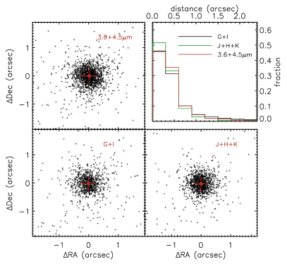
Figure 1.— $\Delta$RA vs $\Delta$Dec for radio–optical/NIR/IRAC matching IDs (upper–left and lower panels). All matchings are shown for each catalog within 2″. In each panel the red points show the median and the errorbars show the $18^{th}$/$84^{th}$ percentiles of the $\Delta$RA and $\Delta$Dec distributions. The upper–right panel shows the histogram of the distances between radio IDs and matched counterparts, independently for each of the three catalogs.

The sky region included in our detection images contains 1930 sources out of the 2055 of the original paper I radio catalog. All three (optical/NIR/IRAC selected) catalogs described in section 3 were used to identify a (optical/NIR/IR) counterpart for the radio sources in the catalog. The radio and optical/NIR/IRAC WCS were first matched by correcting for the mean offsets in $\Delta$RA_{optical-radio} and $\Delta$Dec_{optical-radio}. The scatter in $\Delta$RA_{optical-radio} and $\Delta$Dec_{optical-radio} is $\simeq$0.3″(see figure 1). Then, for each radio source the three catalogs were searched for a match within $1\arcsec$ (with an order of preference 1) optical, 2) NIR, and 3) IRAC. Most of the radio sample was matched with an optical counterpart: out of the whole sample of matched counterparts, the (optical unmatched) NIR counterparts and (optical and NIR unmatched) IRAC counterparts contribute for about 12% and 9%, respectively. However, about 20% of these IRAC counterparts and 40% of these NIR counterparts are located in “bad areas” of the optical detection image, where detection was hampered by bright sources or artifacts. Also, when restricting to the redshift range $0.3<z<1.3$ which will be the main focus in the following, IRAC selected counterparts contribute for just 1%, and NIR selected counterparts for 7% (half of which in bad areas of the optical detection image).

While for most of the sources a counterpart closer than 1″  was found, for almost 6% of the 1930 sources it was not possible to identify a counterpart within $1\arcsec$. Half of these could be matched with a counterpart increasing the matching radius up to $1.5\arcsec$. The other half of the sources without counterpart were automatically and visually inspected: some of these sources are indeed found in image areas affected by bright objects halos/artifacts, some others are blended with another bright object – clearly in such cases the possible counterpart may likely go undetected. However, for 13 (out of 59) unmatched sources it seems that there is actually no counterpart in our images (and no apparent issues in the images which could hamper its detection).

In conclusion, 94% of the radio sources contained in our detection region were assigned a reliable counterpart (within $1\arcsec$), while 3% were assigned a counterpart between $1\arcsec$ and $1.5\arcsec$ and 3% were not assigned any counterpart.

Since the resolution of the radio image is similar to that of the optical/NIR images, we did not apply the likelihood ratio technique (Richter 1975) which is commonly used to evaluate the reliability of each identification based on the source-counterpart distance and counterpart magnitude. However, we used the distance and magnitude distribution of our identified counterparts to evaluate the contamination of our catalog from false counterparts, estimating the probability of false association by randomly shifting the radio source coordinates and repeating the association process. Given the characteristics of most of our associations (75% (97%) are at a distance of less than 0.5”(1”) from the source, 70% brighter than i=25 within an aperture of 1.5”) the overall contamination of the whole catalog is estimated to be lower than 2%. The contamination from false counterparts of the $0.3<z<1.3$ sample which will be used in most part of this work is estimated to be negligible ($<1$%).

Out of the sources with an assigned counterpart, 76% were detected (i.e. have a measured aperture magnitude brighter than mag_cut) in the U band (and up to 80% including objects possibly undetected because in flagged areas of the U band image), 83% (up to 89%) in the g band, 80% (89%) in the r band, 74% (91%) in the i band, 75% (92%) in the z band, 85% (91%) in the J band, 90% (95%) in the H band, 81% (87%) in the K band, 88% (100%) in the IRAC 3.6$\mu$ band, and 93% (100%) in the IRAC 4.5$\mu$ band. We note that we give these numbers as an indication of the typical spectral energy distributions (SEDs) of the radio–selected sample: the specific numbers depend on the different depth and overall quality in terms of bad areas of the different images.

5. Photometric redshifts

5.1. Determination of photometric redshifts from multi–wavelength NUV to mid–IR photometry

The optical, NIR and IRAC selected multi–wavelength catalogs described above were used to estimate photometric redshifts (photo–zs) by means of comparison with a library of galaxy SED templates covering a range of star-formation histories, ages and dust content. A set of 33 templates were used, spanning from a classical local elliptical to several star forming galaxies to a QSO dominated template, and all covering a rest-frame spectral window [1000–70000]$\AA$, thus ensuring an adequate cross-correlation with the available photometric coverage. Beside local galaxy templates (e.g., Coleman et al. 1980, Mannucci et al. 2001, Kinney et al. 1996), a set of semi–empirical templates based on observations plus fitted model SEDs (Maraston 1998, Bruzual & Charlot 2003) of $\approx 300$ galaxies in the FORS Deep Field (Heidt et al. 2003) and Hubble Deep Field (Williams et al. 1996), were included to better represent objects to higher redshifts.

Here we describe briefly the method used to estimate photo–zs, and we refer to Bender et al. (2001), Gabasch et al. (2004) and Brimioulle et al. (2008) for a more detailed description of this method, as well as of the construction of the templates. The aperture PSF-matched photometry of each object in the available (up to 11) passbands was compared with the templates, calculating a redshift probability function over the range $0<z<10$ (in steps of 0.02) for all SEDs. This is done assuming some priors: a different prior on the redshift distribution is assumed for different types of templates (corresponding to younger or older SEDs, that is e.g. an old local elliptical template is assumed to be increasingly unlikely at higher redshifts, while templates corresponding to young stellar populations or QSOs are assumed to have a basically flat likelihood across all redshifts explored). Furthermore, a weak, broad prior on the absolute optical and NIR magnitude lowers the probability to have magnitudes brighter than -25 and fainter than -13. Ly-$\alpha$ forest depletion of galaxy templates is implemented according to Madau (1995). The “best–fit” photo–z $z_{phot}$ is chosen as the redshift maximizing the probability among all templates, and an error on $z_{phot}$ is defined as $e_{zphot}=[\Sigma_{ij}(z_{i}-z_{phot})^{2}P_{ij}]^{1/2}$, with $z_{i}$ the considered redshift steps in $0<z<10$, and $P_{ij}$ the contribution of the j-th template to the total probability function at redshift $z_{i}$.

Systematic offsets between the measured and predicted colors as a function of redshift, which may be due to several reasons as for instance uncertainties in the estimated zero–point, but also possibly uncertainties in the filter response curves or even systematics in the templates, were estimated using almost 500 spectroscopic redshifts available in our field (paper III, private communication from G. Smith 2007, plus some few more published redshifts available from NED). Therefore, the zero–point for each of the passbands was corrected by a factor which minimizes the systematic shift between observed and predicted color for well–fitted spectroscopic galaxies.

Also stellar templates (Pickles 1998) were fitted to all sources. Comparing stellar and galaxy $\chi^{2}$ for objects with a point–like morphology, we checked that objects brighter than I$\simeq$23.7 with a best–fit stellar $\chi^{2}$ lower than the best–fit galaxy $\chi^{2}$ could be classified as stars. The number counts of such selected “stars” are in good agreement with predictions of the Robin et al. (2003) Galaxy model . Fainter than I$\simeq$23.7, the classification was found less reliable. None of the sources in the radio sample was classified as star.

When fitting an object’s photometry, besides excluding from the fit all magnitudes deemed unreliable (including magnitudes of objects in flagged areas), all magnitudes fainter than mag_cut (as defined above) were considered as drop-outs, and a few photo-z determinations with different ways of dealing with drop-outs were compared, in order to test the stability of the derived photo-z. Obviously, the estimated photo-z is most unstable for those objects with a very high number (e.g. $>6$) of drop outs (or combination of drop outs and flagged magnitudes). Only a minor fraction of the objects is concerned, and the effect on the global sample, and in particular at redshift lower than 2, can be considered negligible. Nonetheless, the outcome of this test was used together with the $\chi^{2}$ of the best fit, the error on the estimated photo-z, and on the total number of actually measured magnitudes used (e.g. not upper limits or flagged magnitudes), to evaluate the quality of the estimated photo-z for each source.

Only “constrained photo-zs”, i.e. with at least 4 measured magnitudes actually used (thus not including upper limits and flagged magnitudes) and a discrepancy between different determinations of less than 20% in $\Delta z$/(1+$z$) were deemed reliable^,. In the following we only use photo–zs deemed reliable based on these criteria, unless otherwise noted.

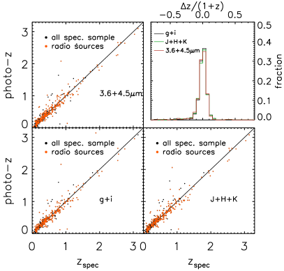
Figure 2.— The comparison of spectroscopic and photometric redshifts for more than 400 sources in the field. In the upper–left and lower panels the estimated photometric redshift is plotted against the spectroscopic redshift, separately for the three optical, NIR and IRAC selected catalogs (the numbers of matched sources are 402, 419 and 429 respectively). The solid line in each panel marks the bisector. Orange symbols highlight radio sources, making up about 3/4 of the spectroscopic sample. The histograms of $\Delta z$/($1+z$) for all three catalogs are plotted in the upper–right panel.

5.2. Accuracy of photometric redshifts

The overall accuracy of our photo–zs is estimated by comparison with the spectroscopic sample. Figure 2 shows the comparison of the spectroscopic redshifts with the retained reliable photo–zs for each of the photometric catalogs (optical, NIR and IRAC selected). In each case, more than 400 objects have been used for the comparison, deriving a median($\Delta z$/($1+z$))$<0.003$, $\approx$3.5% outliers (defined as $\Delta z$/($1+z$)$>0.2$), and an accuracy of $\approx 0.05$ in $\Delta z$/($1+z$), as estimated either from the NMAD estimator (Hoaglin et al. 1983, Ilbert et al. 2009) or from the 16^th-84^th percentiles of $\Delta z$/($1+z$).

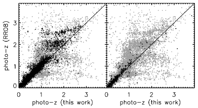
Figure 3.— The comparison of this work photo–zs with those derived by RR08. Left panel: gray symbols show all data points while black symbols show those which in the RR08 catalog have photometry in 6 passbands and mag r$<24$. Right panel: gray symbols show all data points while black symbols show objects with available spectroscopic redshift in either this work or RR08. See text for details.

While we have a sizable spectroscopic sample allowing us to assess the accuracy of our photo–z determination, it may also be useful to compare our results with independently determined photo–zs. While such comparison has not the same strengths of the usual spectroscopic vs photometric redshift comparison, it may help to overcome two of its main weaknesses: spectroscopic samples are typically only a small fraction of a galaxy sample, and are significantly biased toward bright sources. In figure 3 we show the correlation between the photo–zs derived in this work and those derived by Rowan-Robinson et al. (2008) (hereafter RR08). RR08 derived photo–zs for all the SWIRE survey, including the Lockman Hole field used in this work. They not only use a different code for estimating photo–zs , but also a significantly different approach. While having a full optical+NIR coverage in some of the fields, in the Lockman Hole they only use photometry in U, g, r, i, 3.6 and 4.5$\mu$m passbands. They report for the whole SWIRE survey a typical rms of (z_phot-z_spec)/(1+z_spec), excluding outliers, slightly larger than 4% for 6 passbands (which is the case of the Lockman Hole) and r${}_{Vega}<$24, and $\approx$ 4% outliers. In the left panel of figure 3 we thus highlight the comparison for sources with r${}_{Vega}<$24 and photometry available in 6 passbands in the RR08 catalog. By comparing our photo–zs with those by RR08 for these objects, we find almost 6% outliers, a median (z_RR08-z_thiswork)/(1+z_thiswork) of $\approx-0.03$, and a scatter $\approx$6%, which is consistent with what expected based on the claimed scatter of both works. We note that their performance, for all SWIRE fields, worsens for $z>1.5$ (see original paper). In fact, this worsening may be expected to be especially significant for the Lockman Hole where no NIR photometry is used in RR08, thus likely hampering photo–zs at $z>1-1.5$. In fact, as figure 3 shows, the comparison between our and RR08 photo–zs gets significantly worse beyond z$\approx 1.5$. As far as our photo–zs are concerned, for $\approx 15$ objects with $1.5<$z${}_{spec}<3.2$ we have a median (z_phot-z_spec)/(1+z_spec) $\lesssim 0.01$ and scatter $\lesssim 0.05$, pretty similar to the figures for the whole sample, but a formally higher number of outliers ($\lesssim$7%, due to one outlier out of $\approx$15 objects). The right panel of figure 3 highlights instead the comparison of RR08 and our photo–zs for sources with spectroscopic redshift available, either in our catalogs or in RR08. For these sources, while finding a scatter similar to that of the whole magnitude– and number of passbands– limited sample, we find a lower median ($\approx-0.01$), and $<5$% outliers. We notice that the spectroscopic samples used in this work and in RR08 have a significant overlap, thus this might affect the comparison of the photometric redshifts results. Nonetheless, the comparison of photometric redshifts derived with different photometry, different SED libraries, and different methods, allows an indirect evaluation of the photo–z performance on a much larger sample, and at fainter magnitudes, than those allowed by the usual comparison with spectroscopic redshifts. This comparison confirms, at least out to redshift $\sim 1.5$, the overall accuracy of our photo–zs as estimated by comparison with our spectroscopic sample.

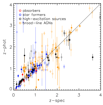
Figure 4.— The comparison of this work photo–zs with spectroscopic redshifts of 198 X–ray sources from the Trouille et al. (2008) sample. Solid symbols refer to a subsample of 71 radio detections, while empty symbols do not belong to the radio sample. The solid line is the bisector. Color coding reflects the Trouille et al. (2008) optical spectral classification as indicated (see text for details).

On the other hand, it is interesting to compare our photo–zs with a spectroscopic sample of X–ray sources in this field published by Trouille et al. (2008). In figure 4 we compare our photo–zs with (Trouille et al. 2008) spectroscopic redshifts for $\approx$200 X–ray sources (out of which $\approx 70$ belong to our radio sample) for which we have a deemed reliable photo–z. We divide and color–code the sample according to the Trouille et al. (2008) optical spectral classification, in absorbers, star–formers, high-excitation sources and broad-line AGNs (see the original paper for details). The fraction of such “peculiar” objects in this comparison sample is quite relevant, with 40% of the sample being made of broad-line AGNs, and a further $\approx$ 30% of high-excitation sources. As figure 4 shows, our photo–zs perform significantly worse for this spectroscopic sample, as compared to our (or RR08) spectroscopic sample, with much larger scatter and number of outliers. The overall statistics for $\Delta$z/(1+z) for this sample is median$\leq-0.015$, NMAD scatter $\approx$10%, and $\approx$20% of the objects having $\Delta$z/(1+z)$>$20%. As it is clear from the figure, the worse results are obtained for the broad-line AGN sub–sample (NMAD scatter $\approx$17%, $\approx$30% of the sample with $\Delta$z/(1+z)$>$20%). The poor agreement obtained from this comparison is not unexpected, due to the contamination of the broad–band photometry with a strong AGN contribution (see e.g. Polletta et al. 2007, Salvato et al. 2009, and references therein). We also note that our photo–zs performance appears to be similar or better than that achieved by Trouille et al. (2008), even though when estimating photo–zs they include templates built from their spectroscopically confirmed broad-line AGNs, while our template set was not specifically tailored toward AGN–dominated SEDs. Furthermore, we note that many (not all though) of the outliers have a large error associated with the estimated photo–z.

5.3. Photometric redshifts for the radio sample

An estimated reliable photo–z is determined for 1610 radio sources (86% of the identified counterparts and 83% of the whole radio sample included in the detection image), while for the rest either no photo–z could be estimated, or in most cases it was deemed not reliable according to the criteria defined above.

In figure 2, the $\approx 300$ radio sources making up about 3/4 of the spectroscopic sample are highlighted with orange symbols. While one might expect a worse performance of the photo–zs for the radio sample, because of the presence of the significant AGN population among radio sources, the statistics for the radio sample alone are quite similar, and only slightly worse, than those obtained using the whole spectroscopic sample: median $\Delta z$/($1+z$)=0.0008, scatter $\approx$5.5%, and 4% outliers (however we note again that a large fraction of the whole spectroscopic sample is made of radio sources). In figure 4 we have already shown (solid symbols) how our radio sample photo–zs perform for the Trouille et al. (2008) X–ray selected sources. In the following, we include the spectroscopic redshifts from Trouille et al. (2008) in our analysis of the radio sample.

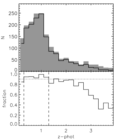
Figure 5.— The redshift completeness of the radio sample. Upper panel: The shaded histogram shows one realization of the redshift distribution of the whole sample of identified counterparts, while the solid line shows the histogram of used redshifts (spectroscopic redshifts or reliable photo–zs). Lower panel: The fraction of available redshifts (spectroscopic redshifts or reliable photo–zs) as a function of redshift: the sample is assumed to be more than 90% complete in the redshift range $0.3<z<1.3$.

In figure 5 we show the redshift completeness of our sample (including spectroscopic and reliable photo–zs) as a function of redshift. Our criteria for selecting a reliable photo–z naturally disfavor higher redshift sources. Since of course we do not know the redshift of all the sources, we can do just an approximate estimate: we assumed that all our photo–zs were broadly correct, even those we decided were unreliable, and used them as a reference to estimate the redshift completeness of the sample. By comparison with our different photo–z catalogs based on different settings (of which figure 5 is one example), we estimated that in the redshift range 0.3–1.3 our redshift completeness should always be higher than 90%, and the $0.3<z<1.3$ sample is overall complete at a 95% level. In other words, if our photo–zs are broadly correct so that the total number of objects in the redshift range $0.3<z<1.3$ is right, we estimate an overall redshift completeness in the $0.3<z<1.3$ redshift range of more than 95% of the identified counterparts, and more than 90% of the whole radio sample within the detection image assuming that all radio sources without an identified counterpart are in this redshift range. This is definitely a conservative assumption since it is likely that many of the unidentified counterparts are very faint galaxies probably at higher redshift.

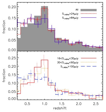
Figure 6.— Top panel: the gray shaded histogram shows the redshift distribution in the range $0.1<z<2.7$ based on the sample of radio sources with identified counterpart and reliable redshift estimate (see text). The red (dotted) and purple (continuous) lines show the redshift distribution of flux–limited samples with radio flux density above 24$\mu$Jy and 84$\mu$Jy, respectively. All distributions are sky-coverage corrected (see text). All histograms are normalized to the total number of objects in each sample. Bottom panel: The red (continuous), yellow (dotted) and blue (dashed) lines show the redshift distributions of sub–samples with radio flux densities in the range [16–30], [30–60], and $>100\mu$Jy, respectively. In both panels, all distributions are sky-coverage corrected (see text), and are normalized to the total number of objects in each sample. Errorbars show Poissonian errors.

5.4. Redshift distribution of the radio sample

In figure 6 we show the redshift distribution of radio sources based on the radio (sub–)sample for which either a reliable photo–z or a spectroscopic redshift is available (gray shaded histogram). The redshift distribution is shown up to redshift $z\sim 2.7$, beyond which the redshift completeness is expected to drop below 80%. The redshift distribution plotted is not corrected for the estimated redshift incompleteness as estimated above (e.g. figure 5).

Since the DSF radio image is obtained with a single VLA pointing, the rms is not constant over the field, but increases with the distance from the field center. For this reason, the whole radio sample does not have a single flux density limit and this needs to be taken into account. In the following, wherever it is needed we will correct the biased nature of the whole sample by taking into account the non–uniform rms. While it is virtually impossible to make a perfect correction, due to the unknown size distribution of the radio sources, for our purpose we will calculate the appropriate correction for all resolved sources for which a reliable size could be estimated, and will assume that all remaining sources have a typical source size of 1.2″(see paper I). Taking into account the bandwidth and time smearing, as well as the primary beam correction, and the resolution of the image where the detection was performed, we can estimate how the rms changes across the image, and thus the 5–$\sigma$ limiting flux density at each distance from the field center (see paper I for more details). In figure 7 we show, as an example, the estimated 5–$\sigma$ limiting flux density as a function of distance from the field center for a source of size$\sim$1.2”. Based on this estimated 5–$\sigma$ limiting flux density as a function of distance, and on the masked areas in the optical/IR detection images, we calculated the area $A_{i}$ over which each object could be observed and enter our sample. The sky coverage is then used to weight each object (by 1/$A_{i}$) and thus estimate properties for a flux–limited sample. We note that, as it can easily be seen from figure 7, the faintest sources in our sample can be observed over a very small fraction of the survey ($<$10%). One might thus be concerned that inaccuracies in the sky coverage correction would significantly affect the results. However, we note that all results presented in the following would be unchanged if considering only flux-limited sub–samples selected in uniformly covered portions of the image (e.g., $R<5\arcmin$ and $S_{1.4GHz}>16\mu$Jy, or $R<20\arcmin$ and $S_{1.4GHz}>84\mu$Jy, see fig.7), while the sky coverage correction allows us to make full use of our data set. In the following, we will explicitly refer to flux–limited samples when using sky-coverage corrected samples, in contrast with the whole, biased sample.

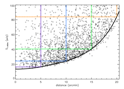
Figure 7.— The solid line shows the 5–$\sigma$ limiting flux density as a function of distance from the center of the VLA field, for a source size of 1.2” (see text for details). Empty symbols show the integrated flux density vs. distance from the field center for actual detections. Thick dotted lines of different colors show four examples of flux-limited sub–samples selected in uniformly covered portions of the image ($R<5\arcmin$ and $S_{1.4GHz}>16\mu$Jy, $R<10\arcmin$ and $S_{1.4GHz}>24\mu$Jy, $R<15\arcmin$ and $S_{1.4GHz}>41\mu$Jy, and $R<20\arcmin$ and $S_{1.4GHz}>84\mu$Jy).

All distributions plotted in figure 6 are corrected by the sky coverage. Beside the redshift distribution derived from the whole sample, in the top panel of figure 6 we also show the redshift distributions of two flux–limited samples with $S_{1.4GHz}>$24 and $>$84 $\mu$Jy. These suggest that the redshift distribution might depend of the flux density of the sample, and we try to make this clearer in the lower panel of figure 6, where we plot the redshift distributions of three sub–samples in different flux density ranges, our faintest sources (16.5$<S_{1.4GHz}<$30 $\mu$Jy), our typical about–median flux population (30$<S_{1.4GHz}<$60 $\mu$Jy), and bright sources ($S_{1.4GHz}>$100 $\mu$Jy). The redshift distribution of the faintest sources seems to be different from that of the bright ones, with a sharper peak at $z\approx 0.9$. A Kolmogorov-Smirnov test indeed suggests that the two distributions are different at a high significance level ($P\leq 0.005$).

6. Spectral energy distribution fitting

We use SED fitting on the available multi–wavelength photometry in order to estimate fundamental properties of the stellar populations hosted in this radio source sample. In the following we will consider photo–zs just as spectroscopic redshifts, assuming that the galaxy is at that redshift and ignoring any error on the photo–z. Different SED fits are used in the following. The first characterization of each galaxy SED is given by the best–fit template associated with the best–fit photo–z. As already said above, and as will be described more in detail below, the templates span a range in stellar population ages, including dust extinction. These templates will then be used to classify galaxies according to the broad, average properties of their stellar populations. In order to properly treat galaxies with an available spectroscopic redshift, the fit was recomputed for these objects assuming the spectroscopic redshift.

In order to classify SEDs based on a more “parametric” approach, and also to investigate possible misinterpretations coming from the use of non–evolving templates, we also performed SED fits using stellar population synthesis models produced with the Bruzual & Charlot (2003) code. Star formation histories (SFHs) were parametrized by simple exponentially declining star formation rates, with a timescale $\tau$ ranging between 0.1 and 20 Gyr, and age between 0.01 Gyr and the age of the Universe at the object’s redshift. Metallicity is fixed to solar and a Salpeter (1955) initial mass function is adopted, with lower and upper mass cutoffs of 0.1 and 100 M_⊙. A variable amount of extinction by dust is also included, with $A_{V}$ $\in[0,1.5]$. The fitting procedure is described in full detail in Drory et al. (2004, 2005). These results too will be used in the following to roughly characterize the host stellar populations based on the best–fit age/$\tau$ (meaning the age of the stellar populations from the onset of the star formation divided by the e–folding time of the exponentially declining SFH).

Finally, SED fitting is also used to estimate stellar masses. For this purpose we use, as it is customary, a two-component model, adding to the main smooth component (exponentially declining SFHs described above) a secondary burst. This burst is modeled as a 100 Myr old constant star formation rate episode. Metallicity and IMF of the burst are the same assumed for the main component, however dust extinction for the burst is allowed to reach higher values ($A_{V}$ $\in[0,2]$). We notice that since we fit aperture photometry, the stellar masses obtained refer to the portion of the galaxy contained in the aperture. We correct these masses to “total stellar masses” by means of the ratio of “total” (FLUX_AUTO) and aperture fluxes in the detection images. The median correction applied for the radio sample is a factor $\approx 2$, and 90% of the sample is corrected by a factor ranging between 1.5 and 4. This is an approximation neglecting any color gradients which may certainly exist in the galaxy, in other words we assume that the stellar populations within the measured aperture are representative of the stellar populations of the whole galaxy.

Some of the main derived properties which are used in this work, for objects with spectroscopic or reliable photo–z, are listed in Table 2 which is available in full on the on–line version.

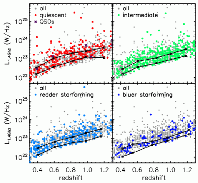
Figure 8.— The 1.4 GHz luminosity plotted against redshift for objects with redshift between 0.3 and 1.3. Grey points in all panels show all data points while colored symbols show objects whose photometry was best–fitted by SEDs of different types, as indicated in each panel. In each panel, connected small squares show the (sky coverage corrected) interquartile range of the $L_{1.4GHz}$ distribution as a function of redshift for the relevant SED–selected sub–sample.

7. SED properties of host galaxies: AGN activity and star formation

In the following we compare the radio and optical/NIR properties of this radio sample based on the SED fitting results described above.

As shown in figure 8, galaxies best–fitted by different kind of templates (thus in principle galaxies with different stellar populations) tend to occupy different locations in the radio luminosity against redshift diagram. The simplest, and expected, explanation is that different radio luminosities are associated to different physical processes, namely star formation and AGN activity. Figure 8 shows the radio luminosity against redshift for classes selected based on the best–fit photo–z SED template. The templates were divided in “quiescent” (including for instance the elliptical template by Coleman et al. (1980) and the S0 and Sa templates by Mannucci et al. 2001), “intermediate” galaxies with low star formation (including e.g. the Sb Mannucci et al. (2001) template), and “star–forming” templates including all actively star–forming galaxies, plus a “QSO” class of a few objects best–fitted by a QSO template. As a reference, the restframe U-B color ranges for the three classes of quiescent, intermediate, and star–forming objects are approximately 1.1–1.4, 0.9–1.1, 0.1–0.9, respectively. Similarly, the U-V color ranges are approximately 1.9–2.2, 1.5–1.8, 0.1–1.3, while the break strengths at 4000$\AA$, $D_{n}(4000)$ , are about 1.6–2.1, 1.5–1.7, 1–1.3. For reference, these $D_{n}(4000)$ ranges may be compared for instance with typical $D_{n}(4000)$ values for different kinds of stellar populations measured in a local (SDSS) sample (Gallazzi et al. 2005, their figure 7), and in a VVDS sample in the redshift range $0.45<z<1.2$ (Franzetti et al. 2007, their figure 4). We also note that in figure 8, the “star–forming” class is further split in two sub–classes of star–forming templates, “redder SF” and “bluer SF”, with restframe U-B ranging in 0.7–0.9 and 0.1–0.7, and $D_{n}(4000)$ about $\approx$1.3, 1–1.2, respectively.

Due to the non–evolving nature of the templates used in the photo–z determination, figure 8 only shows the stellar populations status (i.e. actively star–forming, passively evolving, etc.) at the time of observations, without any evolutionary link between same–class objects at different cosmic epochs. In other words, depending on the specific star formation history of each galaxy, and on the overall evolution of galaxy stellar populations, galaxies may (and will) change their class as time goes by.

As figure 8 shows, at all redshifts the highest radio luminosities in the probed range (e.g. L${}_{1.4GHz}>2\times 10^{23}$ W/Hz at $z\sim 0.5$ or L${}_{1.4GHz}>5\times 10^{23}$ W/Hz at $z\sim 1$) are typical of low–starforming systems (i.e., galaxies classified as intermediate or quiescent). Nonetheless, radio luminosities of such low–starforming galaxies span all the range covered by this survey. On the other hand, galaxies classified as actively star–forming tend to avoid the highest radio luminosities, with just few exceptions. The median radio luminosities of all sub–samples are similar, with star forming galaxies typically showing a median radio luminosity about 20% lower than low-starforming systems (quiescent and intermediate), over the redshift range probed. However, the mean radio power of intermediate and star forming galaxies is typically lower than that of quiescent galaxies (the mean L_1.4GHz of bluer star–forming, redder star–forming, and intermediate galaxies are 30%, 40%, and 50% of the mean L_1.4GHz of quiescent classified sources, respectively). The interquartile ranges for L_1.4GHz plotted in figure 8 also show how the typical range and spread in radio power is different for different SED classes, with the bluer star–forming galaxies mostly lying just above the flux density limit of this survey.

Finally, figure 8 shows how a significant part of this radio sample is made of objects classified as intermediate. This is likely due to the depth of this survey which allows us to go beyond the AGN dominated population, but at the same time does not allow us to reach the still fainter radio luminosities typical of the bulk of normal star–forming galaxies. We note that, while the statistics given above take into account the sky coverage, the points plotted in figure 8 show the whole radio sample with $0.3<z<1.3$, regardless of the different sensitivity at different radii in the VLA image, therefore the different densities of data points are not directly indicative of the actual relative fractions of different kinds of objects, which are better addressed below.

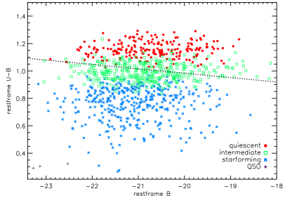
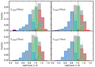
Figure 9.— Top panel: The restframe U-B vs B color–magnitude diagram for objects with redshift $0.3\leq z\leq 1.3$. All objects are included regardless of their radio flux density and position in the VLA image. Symbols are color coded according to best–fit SED type, as indicated (same broad classes as in figure 8). The dotted line shows the division between red sequence and blue cloud from DEEP2 data as in Willmer et al. (2006), Cooper et al. (2007). Bottom panels: The distribution of restframe color U-B for the different SED classes, in four flux–limited sub–samples, as indicated (see text for details). The dotted lines mark the U-B color of the division line at the median B magnitude of each plotted sample. In each panel, histograms for the different SED classes are color–coded as in the upper figure (quiescent = horizontal, intermediate = diagonal and star–forming = vertical hatched), and the gray–shaded histogram shows the distribution of the whole subsample plotted in the panel.

7.1. The nature of faint radio sources: a significant intermediate population?

In figure 9, we show the restframe U-B vs B color–magnitude diagram of the radio sample, divided as above in quiescent, intermediate and star–forming. In this figure, all sources with redshift $0.3<z<1.3$ are plotted, taking advantage of the small evolution of the restframe U-B color in the redshift range probed, and thus just one separation between red and blue galaxies was adopted at all redshifts (see e.g. Willmer et al. 2006, Cooper et al. 2007, in the same redshift range studied here). The figure shows the well known different locations in the color–magnitude diagram of different galaxy types, with quiescent galaxies on the red–sequence and star–forming galaxies in the blue–cloud. However, as compared to a typical color–magnitude diagram for an optically selected galaxy sample, it is evident that the so–called “green valley”, often thought to be populated by transitional objects which are shutting off their star formation and migrating to the red sequence, is not an underpopulated region in this diagram, and actually contains a significant fraction of this radio–selected sample.

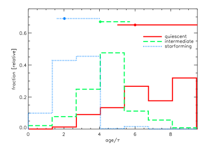
Figure 10.— The age/$\tau$ distribution for the sub–samples of quiescent, intermediate, and star–forming objects. The solid symbols and errorbars on top of the histograms show the median and 16^th-84^th percentiles of each distribution. Age/$\tau$ values larger than 9.5 were set to 9.5 for the purpose of this plot.

However, the actual nature of this significant population of apparently intermediate–type galaxies with low star–formation activity is not necessarily clear. In fact, while it might be tempting to consider the option that these are indeed “composite” or “transition” systems, meaning galaxies shutting off their star formation because of (or linked to) an host AGN, on the other hand the colors characteristic of an “intermediate” SED can also be produced in other ways, the most obvious being a starburst affected by a very high dust extinction which is not properly handled by our template set, or possibly a red–sequence galaxy whose observed SED is severely contaminated by AGN emission. In fact, in an attempt to look a bit further into the dust attenuation issue of the intermediate galaxies, we can compare our template–based classification with the parametric one based on the single–component model SED fitting. As shown in figure 10, there is a good overall correlation between the age/$\tau$ of the best–fit model and the template–based classification. However, if we look at the dust extinction which according to the best–fit is affecting the model SED, we find that 10% of the intermediate sample at $0.3<z<1.3$ was best–fitted by a significantly extincted young stellar population (age/$\tau<4$, $A_{V}>1$). For comparison, 30% of the galaxies classified as star–forming was best–fitted by such kind of model, and 3% of the galaxies classified as quiescent. Even though we will not attempt to correct colors based on the rough attenuation estimated by this simple SED fit, the occurrence of apparently significantly extincted objects in the intermediate sample may suggest a possibly relevant contamination by reddened starbursts (see also e.g. Cowie & Barger 2008). The actual nature of these intermediate sources will be further investigated in a forthcoming paper, by exploiting X–ray and infrared data.

For the time being, to avoid misinterpretations, in the following we will drop the labeling of the three classes as quiescent, intermediate, and star–forming, which directly refers to the inferred nature of the host stellar populations, and will adopt a more generic and observationally–based “red”, “green” and “blue”.

It is worth noticing how the nature of the radio–galaxies host stellar populations significantly depends on the flux densities reached by the radio survey. In the lower panels of figure 9 the sample plotted in the upper panel has been split in order to draw more meaningful conclusions on the stellar populations of flux–limited radio–selected sub–samples. As it is evident from figure 9, and as it is expected (see section 1), the stellar population properties of the host galaxies, and thus likely also the process responsible of the radio emission, are different in different radio flux density ranges. In the shallowest sample considered ($S_{1.4GHz}>84\mu$Jy), the fractions of blue, green, and red classified objects are roughly similar (33%, 36%, 30%, respectively); in the $S_{1.4GHz}>40\mu$Jy and $S_{1.4GHz}>24\mu$Jy samples they are about 40%, 40%, 20% , and eventually they become 45%, 33%, 22% in the deepest radio sub–sample ($S_{1.4GHz}>16\mu$Jy). This clearly suggests how the contributions of the actively star–forming and red galaxies change with the limiting flux density of the sample, with red galaxies increasing their relevance in brighter samples and, viceversa, star–forming galaxies becoming more important in fainter samples. For these flux–limited samples, according to a Kolmogorov–Smirnov test, the U-B color distributions of the radio–faintest and brightest sub–samples are different at a $\simeq 98\%$ significance level. However, the significance of the change in the colors of the host galaxies at different radio flux densities is obviously more evident when considering sources in ranges of radio flux density instead of flux–limited samples, as we will do in the following.

We should notice that, since the lower panels of figure 9  refer to a flux–limited sample, there are different effects which come into play in realizing the different distributions of the different–depth sub–samples, as for instance the higher fraction of $z\simeq 1$ as compared to $z<0.5$ objects probed at fainter flux densities (see figure 6), and likely an evolution with redshift of the 20cm luminosity threshold between star formation–dominated and AGN–dominated radio samples (see figure 8). This is further discussed below.

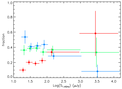
Figure 11.— The relative contributions of different SED–classified samples as a function of radio flux density. The points show the median 20cm flux density in the flux bin (indicated by the horizontal error bar) against the fraction over the whole population in that flux bin. Color coding is the same as in figure 9. The flux density bins for the different SED–classified samples are the same, but are shown with a small offset in the figure for clarity.

The different (sky–coverage corrected) contributions of the red, green, and blue classified sources are shown in figure 11. This figure shows how the $S_{1.4GHz}\geq 100\mu$Jy sources, which have a relatively flat redshift distribution in the redshift range we are probing (fig. 6), are roughly equally split between the three sub–classes of red, green and blue galaxies. When going to fainter flux densities, where we saw that the redshift distribution becomes more skewed toward higher redshifts, figure 11 shows that the sample is depleted of red galaxies while the fraction of blue actively star–forming systems increases (green–classified objects make up $\approx$30-40% in all sub–samples). In the faintest subsample, with $S_{1.4GHz}$ in the range 16–25$\mu$Jy, less than 25% of the $0.3<z<1.3$ sample is at $0.3<z<0.7$, compared to more than 40% in the shallow $S_{1.4GHz}\sim 100\mu$Jy subsample; the faintest sample only hosts $\sim$10% red galaxies, while the fraction of blue galaxies has increased to more than 50%. According to a Kolmogorov–Smirnov test for these radio–faintest and brightest samples, the U-B color distributions are different at a $>$99.7% significance level.

We also note that, by splitting host galaxies just based on their U-B restframe color (e.g., red galaxies with U-B$>$1, blue galaxies with U-B$<$1) we find that, in agreement with previous work (e.g. Mainieri et al. 2008), the radio population is dominated by red galaxies above flux densities of 100$\mu$Jy, while below 80$\mu$Jy blue galaxies begin to dominate ($\approx 65$%, considering a flux–limited sample with $40<S_{1.4GHz}<80\mu$Jy). Splitting this sample in three redshift bins with $0.3<z<0.6$, $0.6<z<0.9$ and $0.9<z<1.3$, we find that this $\approx 65$% fraction stays basically constant as a function of redshift. However, we should think in terms of luminosities instead of flux densities: while the flux density range $40<S_{1.4GHz}<80\mu$Jy at $z\sim 0.3$ corresponds to a luminosity range of approximately 1–3$\times$10²²W/Hz, at $z\sim 1.3$ it corresponds to luminosities of order 3–6$\times$10²³W/Hz. These $\sim$10²³W/Hz luminosities in the lowest redshift bin would correspond to flux densities well above 100$\mu$Jy, which as we said are usually dominated by red galaxies. Therefore, the apparently mild evolution between redshift $z\sim 0.5$ and $z\sim 1.1$ of the fraction of blue galaxies in $S_{1.4GHz}<80\mu$Jy samples actually happens against a change in radio luminosities of an order of magnitude. This is due to evolution in these faint populations as we will further discuss below (section 7.2).

In the following we compare our SED–selected subsamples in terms of different classification criteria from previous studies.

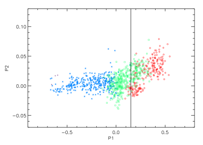
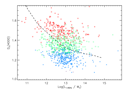
Figure 12.— Top panel: The principal restframe color–color diagram (P1,P2) for objects with redshift $0.3\leq z\leq 1.3$. Symbols and color coding are based on the best–fit SED type as in figure 9. The solid black line shows the color–cut P1=0.15 between AGN and star–forming dominated populations used in Smolčić et al. (2008). Bottom panel: The $D_{n}(4000)$ index plotted against the radio luminosity per unit stellar mass, for objects with redshift $0.3\leq z\leq 1.3$. Symbols and color coding as in figure 9. The dashed line shows the separation between AGN and star–forming galaxies as defined in Best et al. (2005b). For the purpose of this plot stellar masses were scaled to a Kroupa (2001) IMF.

7.1.1 NUV/optical vs radio properties

For the sake of comparison, we show in figure 12 how our classification based on the observed broad–band SED compares to two different classifications of radio samples based on specific rest–frame properties. In the top panel of figure 12 we compare with the AGN/star–forming classification used in Smolčić et al. (2008). Based on a SDSS/NVSS/IRAS sample of local radio sources, Smolčić et al. (2006, 2008) devised a classification method to separate populations of radio sources whose 1.4GHz emission is dominated by AGN, by star formation, or is likely to be contributed by both processes. This is based on the principal component restframe colors P1 and P2, which are linear combinations of restframe colors in the modified Strömgren system in the wavelength range 3500 – 5800 $\AA$ (Odell et al. 2002, Smolčić et al. 2006). In Smolčić et al. (2008), a color cut at P1=0.15 was adopted to separate their radio sample in the COSMOS field into two populations of AGN and star–formation dominated systems. As the figure shows, indeed also our objects with a P1$>0.15$ are mainly classified as quiescent (thus likely with an AGN produced radio emission), or at most as intermediate color sources (thus with a possibly relevant contribution by AGN). On the other hand, our class of intermediate objects extends down to slightly below P1=0, where increasingly star forming populations become dominant extending down to P1$\approx-0.7$. Thus, to first approximation, most of our green objects would be classified as star–forming in this scheme. Nonetheless, from e.g. Smolčić et al. (2006), we note that a significant fraction of the sources with P1 around zero (roughly $-0.1<$P1$<0.1$) populates the region in the BPT (Baldwin et al. 1981) diagram where the AGN/star–forming classification is considered uncertain.

In the bottom panel of figure 12 we plot instead our sample in the Log(L${}_{1.4GHz}/M_{*}$) vs $D_{n}(4000)$ plane. Best et al. (2005b) divided a sample of SDSS/NVSS matched sources at redshift $z<0.3$ into two broad classes of AGN and starbursting galaxies. The selection was in fact based on the 4000$\AA$ break index $D_{n}(4000)$ and radio luminosity per unit stellar mass L${}_{1.4GHz}/M_{*}$. Since we don’t have spectra for all sources in our sample, we use synthetic $D_{n}(4000)$ indices derived from best–fit stellar population synthesis models, which may only be considered as a very approximate estimate of the real $D_{n}(4000)$. We use the stellar masses described above to calculate L${}_{1.4GHz}/M_{*}$ for each galaxy. If the estimates we plot are representative enough of the true $D_{n}(4000)$ and L${}_{1.4GHz}/M_{*}$, we should conclude that indeed basically all of our blue objects are below the Best et al. (2005b) division line, and the vast majority ($>$90%) of the red galaxies are above the line. The green sources fill the gap between the two, just about the division line, falling in both the “AGN” and “starburst” regions.

Finally, we show in figure 13 how our classification of this sample compares with other galaxy populations with regard to radio/UV flux densities. Figure 13 shows for our sample the star formation rate (SFR), as determined from the 1.4GHz luminosity, against the dust attenuation estimated as A${}^{*}_{2800}\equiv$2.5Log(SFR_radio/SFR_UV). We note that the meaning of these quantities for the whole sample is ill defined. In fact, only for galaxies whose radio emission is due to star formation the quantity plotted as “SFR” actually represents the SFR, and A${}^{*}_{2800}$ indeed is the dust attenuation. Instead, galaxies hosting a radio emitting AGN have their 1.4GHz luminosity at least partially contributed by the AGN, and thus both “SFR” and A${}^{*}_{2800}$ lose their meaning for these objects. However, keeping this in mind, this plot allows us to compare in a simple way our sample with other populations of star forming galaxies at different redshifts and selected with different criteria.

As the figure shows, the range of attenuations derived for our blue objects is in very good agreement with other studies of different kinds of star forming galaxies at different redshifts (Calzetti et al. 2000, Calzetti 2001, Hopkins et al. 2001, Afonso et al. 2003, Choi et al. 2006, Pannella et al. 2009). While part of the green objects would also overlap with these samples, it is clear how the A${}^{*}_{2800}$ for the green population generally lies above the expectations, and definitely the red population has too high values of A${}^{*}_{2800}$. This might support the idea that the red population is for the great majority made of AGN hosts, and also suggest that at least part of the green population has a contribution from AGN to the radio luminosity, even though part of these galaxies can still be very dusty systems.

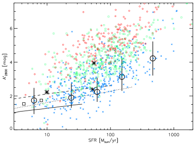
Figure 13.— The “dust attenuation” A${}^{*}_{2800}$=2.5Log(SFR_radio/SFR_2800Å) against “star formation rate” as determined from the 1.4GHz luminosity (see text for the actual meaning of the two quantities plotted). Small symbols color coded as in figure 9 show the $0.3<z<1.3$ radio sample (21 objects (out of which $>$95% are red or green) with A${}^{*}_{2800}>7.5$ and/or SFR${}_{radio}>2000$ are not shown). Large empty circles with errorbars show the Pannella et al. (2009) results (median and 16-84^th percentile range) for star forming BzK galaxies at $z\approx 2$. Empty squares and stars show local galaxies from Calzetti et al. (2000), Calzetti (2001) (star symbols are for galaxies classified as dust–rich in Calzetti (2001); note NCG 1614 with SFR=55M_⊙/yr and very high dust extinction, which by the way hosts an obscured AGN (e.g., Guainazzi & Bianchi (2007))). The solid, dotted and dashed lines show the dust attenuation as a function of SFR as derived from the local optical/UV–selected sample of Hopkins et al. (2001), the intermediate redshift NIR/MIR–selected sample of Choi et al. (2006) and the low–redshift radio–selected sample of Afonso et al. (2003), respectively (see text for details).

The significant occurrence of AGN hosts among the intermediate population between red and blue galaxies has been noted in several previous studies (e.g., Choi et al. 2009, Martin et al. 2007, Nandra et al. 2007, and references therein), as well as their actual nature of composite (meaning SF+AGN) systems (Schawinski et al. 2007, Wild et al. 2007, Salim et al. 2007). We note that the classification of such composite sources in the literature is quite variable, and for instance galaxies with more than 10% of their radio luminosity contributed by star formation have been classified, in some cases, as starbursts (Tasse et al. 2008). This may indeed be the case, and certainly also in our green sample different amounts of star formation are presents, however a starforming–or–AGN classification may be not appropriate for these sources, especially depending on the kind of study they are used for.

7.1.2 Radio–IR properties

As discussed above, in spite of the insight that we can certainly gain by combining radio fluxes and optical/NIR photometry, the results presented so far may not provide conclusive evidence about the actual nature of these sources. Therefore, we need to introduce further information which may help us identify which process powers the radio emission. Obvious promising data already available on this field are X–ray (Chandra) and infrared (Spitzer and Herschel) observations. While we postpone a full analysis of these data to a future work, we use here just the Spitzer/MIPS 24$\mu$m data to estimate the total infrared (IR) luminosity of our sources and thus examine the behavior of our SED–selected sub–samples with respect to the FIR–radio correlation (e.g., Condon 1992, Yun et al. 2001). The DSF was observed at 24$\mu$m with MIPS onboard Spitzer as part of the GO–3 program #30391 (PI: F. Owen), for a total of 60.6 hours over an area of about half square degree, and a median integration time per pixel of about 2500s. The $5\sigma$ flux density limit is estimated to be about 40$\mu$Jy. The data reduction and catalog production are described in full detail in a forthcoming companion paper (Owen et al., in preparation). More than 80% of the faint radio sources from the 90% complete sample in the redshift range $0.3<z<1.3$ are detected at 24$\mu$m. Matched sources with flux possibly contaminated by neighbors within the 24$\mu$m PRF are estimated to be about 10% of all matched detections, based on the cross–correlation with the IRAC 3.6$\mu$m catalog. While upper limits make up for $<20\%$ of the whole $0.3<z<1.3$ sample, they are more relevant for red–classified objects (almost 40% of upper limits) than for green and blue sources.

In the redshift range $0.3<z<1.3$, the observed 24$\mu$m light probes the restframe $\sim 10-20\mu$m. We use the templates of Chary & Elbaz (2001) to estimate from the 24$\mu$m flux density the total (8-1000$\mu$m) IR rest–frame luminosity (or an upper limit for 24$\mu$m–undetected sources). This is done taking the template whose predicted luminosity at the observed 24$\mu$m is closest to the actual observed 24$\mu$m luminosity. Taking the mean or median luminosity across the whole template library typically changes this number within about 0.15dex, but since this is obviously library–dependent we don’t see a real point of adopting the mean or median instead of the formal best–fitting template. Furthermore, even just based on the templates available in this library, such estimate of the total IR luminosity based on the single observed 24$\mu$m point may be affected by systematics of up to a factor 2.

We use this total IR luminosity together with the 1.4GHz luminosity to estimate the logarithmic ratio of bolometric IR and monochromatic radio luminosities $q_{IR}$=Log($L_{IR}/(3.75\cdot 10^{12})$) - Log($L_{1.4GHz}$) (Helou et al. 1985). This is plotted as a function of redshift for the different sub–samples of red, green, and blue sources, in the bottm-left panel of figure 14. In this figure, filled circles show sources unambiguously matched with a 24$\mu$m source, and filled triangles show sources matched within 2” with a 24$\mu$m source but whose 24$\mu$m flux might be contaminated neighbors. Finally, upper limits are shown by down–pointing arrows.

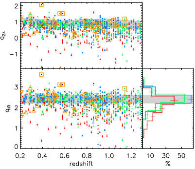
Figure 14.— Bottom panels: in the left panel the flux ratio $q_{IR}$ is plotted against redshift for the different SED–selected sub–samples (color coding as in figure 9). Filled circles show unambiguously matched $24\mu$ sources, filled triangles show matched $24\mu$ sources whose flux might be contaminated by neighbors, and arrows show upper limits (see text for details). Large orange symbols show matched X–ray sources from the Trouille et al. (2008) sample (according to the Trouille et al. (2008) spectral classification, circles, downward triangles, triangles and squares show absorbers, star formers, high–excitation sources and broad–line AGNs, respectively). The gray–shaded area shows the $1\sigma$ range about the (redshift independent) $q_{IR}=2.4$ reported in Ivison et al. (2009). The right-hand panel shows the sky–coverage corrected distributions of $q_{IR}$ for the sub–samples plotted in the left panel, including upper limits (see text for details). The histograms for the red, green, and blue samples are evaluated in the same $q_{IR}$ bins, but are shown slightly offset for clarity. Top panel: same as bottom left panel, but for the observed (non k–corrected) flux density ratio $q_{24}$. The gray shaded area shows the envelope of Chary & Elbaz (2001) and Rieke et al. (2009) templates with $L_{IR}$=10${}^{11}L_{\odot}$ and 10${}^{12}L_{\odot}$ (plus 10${}^{10}L_{\odot}$ for $z\lesssim 0.5$).

The bottom-right panel of this figure shows the $q_{IR}$ distribution (corrected for the sky–coverage) for the three different red, green, and blue sub–samples. It is important to note that the plotted histograms (as well as the related statistics given below) include both 24$\mu$m detections and upper limits. This does not affect our results (or actually affects our conclusions in a conservative way), since we are interested in the difference between the $q_{IR}$ distribution of the three sub–samples, with $q_{IR}$ of intermediate and quiescent sources expected to be lower than $q_{IR}$ of star forming sources, if the radio power of objects classified as intermediate and quiescent is at least partially provided by an AGN. This means that, including upper limits (and possibly contaminated 24$\mu$m detections), we are – if anything – reducing the actual difference between the $q_{IR}$ distributions of the three sub–samples.

In both panels, the gray–shaded area shows the $1\sigma$ range about the (redshift independent) $q_{IR}=2.4$ reported in Ivison et al. (2009). As figure 14 shows, blue star–forming sources mostly lie on the expected FIR–radio correlation. Also up to 50% of the green sources lie within $1\sigma$ of the expected FIR–radio correlation, which would point toward these being powered by star formation as well. However, even though with a broader distribution, red sources also lie close to the FIR–radio correlation, with up to 40% of this sub–sample lying within 1$\sigma$ of the correlation. Sources populating the gray–shaded area in figure 14 (1$\sigma$ about the expected correlation) are for more than 50% classified as star–forming, but show a sizable fraction of $\sim 30\%$ and $\sim 10\%$ of green and red sources, respectively. The $q_{IR}$ distribution of red sources appears to be very different from those of blue and green sources. Even though a Kolmogorov-Smirnov test cannot be meaningfully applied to the sky–coverage corrected distributions, applying it to flux–limited sub–samples selected in portions of the radio image with depth uniformly better than a given threshold, suggests than the $q_{IR}$ distribution of red sources is different at a significance of more than $99.9\%$. A $\chi^{2}$ test on the binned distributions (including errors) plotted in figure 14 (as well as on similar distributions binned with half bin size), also suggests that the distributions of $q_{IR}$ of red vs. blue or green sources are different at a $>99.5\%$ level. On the other hand, the $q_{IR}$ distributions of blue and green sources look much more similar. The $\chi^{2}$ test on the binned distributions suggest that they are different at a $\gtrsim 98\%$ level, and the Kolmogorov-Smirnov test on a limited part of the sample (as above) gives a $P_{KS}\sim 0.2$, thus based on the present data these distributions are, at most, marginally different.

Based on these results one might thus conclude that a large fraction of our sources with intermediate colors, as well as a sizable fraction of the red ones, are actually reddened starbursts. On the other hand, we also note that among the sources which are X–ray detected (and mostly AGN classified in the Trouille et al. (2008) sample), many lie on the FIR–radio correlation, including some classified as absorbers (based on OII or H_α+NII equivalent widths). Indeed, other studies have found that sources classified as low–radio power AGN may often lie on or close to the same FIR–radio correlation expected for star forming sources (e.g. see discussions and references in Smolčić et al. 2008, Sargent et al. 2010). However, it should also be noted that an AGN selected based on its (spectral or photometric) optical/NIR properties (or X–ray), hosted in a “composite” system with ongoing star formation, may be in a stage where radio emission is negligible and thus does not significantly affect the IR/radio properties which remain determined by the star formation process. In this case, while information at other wavelengths suggest the presence of an AGN, it might not (significantly) contribute to the radio power of the source. Furthermore, obscured star formation confined in limited areas of a galaxy might also determine its IR/radio properties while possibly going undetected in broad–band photometry at optical wavelengths. On the other hand, we remind again the reader that the $q_{IR}$ in figure 14 relies uniquely on the observed 24$\mu$m flux density, and thus might be biased producing a spurious result. For comparison, we also show in the top panel of figure 14 the observed (non k–corrected) flux density ratio $q_{24}=Log(S_{24\mu m}/S_{1.4GHz})$. As a reference, the gray shaded area shows the envelope of Chary & Elbaz (2001) and Rieke et al. (2009) templates with $L_{IR}$=10${}^{11}L_{\odot}$ and 10${}^{12}L_{\odot}$ (plus also 10${}^{10}L_{\odot}$ for $z\lesssim 0.5$). This $q_{24}$–based figure essentially reflects the results of the bottom panel. We will continue the investigation of IR/radio properties of this sample with a proper SED analysis of the full data in a future work.

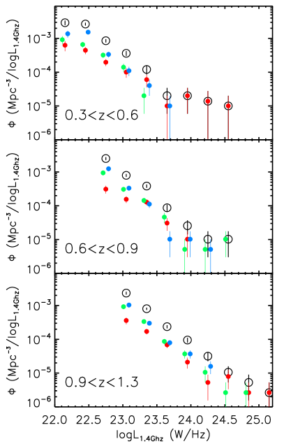
Figure 15.— The 1.4GHz luminosity function of different galaxy classes. Large empty symbols refer to the whole populations, while filled symbols and their coding refer to the same classes as in figure 9. Number densities are shown in three redshift ranges, as indicated. The luminosity functions for the different samples are evaluated in the same $L_{1.4GHz}$ bins, but are shown slightly offset for clarity. Errorbars show Poissonian errors.

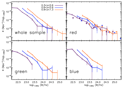
Figure 16.— The redshift evolution of the 1.4GHz luminosity function of galaxies in different SED classes, as indicated in each panel. Luminosity functions are the same as those plotted in figure 15. Different colors refer to different redshift ranges, as also indicated. Errorbars show Poissonian errors. Small squares (with same color coding as solid lines) show, as a reference, the LF of radio–selected AGN as derived by Smolčić et al. (2009b) in similar redshift bins (see text for details).

7.2. Luminosity functions and evolution of faint radio populations

Finally, we investigate the contributions of the different galaxy classes to the sub–mJy population by plotting in figure 15 the 1.4GHz luminosity functions (total and split by SED class) in three redshift ranges. Figure 15 shows number densities based on the $0.3<z<1.3$, $90\%$ complete sample, estimated with the 1/V_max method (Schmidt 1968, Avni & Bahcall 1980). Within the redshift range $0.3<z<1.3$, the maximum volume over which an object can enter our sample essentially depends on its radio luminosity and on the (non uniform) depth of the 1.4GHz image. Therefore, for each source of a given radio luminosity $L_{1.4GHz}$, the maximum volume accessible to the source was calculated, based on the maximum redshift out to which the source would have been detected as a function of the varying image depth of the 1.4GHz image. We remind the reader that, similarly to what discussed above concerning the sky coverage correction, the 1/V_max correction is not negligible for low–luminosity sources due to the limited survey area probing the faintest fluxes. On the other hand, we also note here that luminosity functions obtained, without the use of the 1/V_max correction, by using smaller volume limited samples defined in portions of the radio image and luminosity ranges, are generally in very good agreement with those determined with the 1/V_max method, and lead to the same conclusions.

Only sources in the $>90\%$ complete sample were used, and no further correction was adopted for the small residual incompleteness of the sample. However, we remind the reader again that the $>90\%$ completeness level of this sample was estimated based on some assumptions (as discussed in section 5.3).

Figure 15 shows the relative contributions of the different SED–classified sub–samples as a function of redshift and luminosity. It also suggests an evolution of the luminosity functions of all classes over the probed redshift range, which is shown more clearly in figure 16. This is confirmed by a $\chi^{2}$ fit to the binned data in the three redshift bins with a parametric LF of the Saunders et al. (1990) form $\Phi(L)=\Phi^{*}(L/L_{*})^{1-\alpha}$exp$(-0.5\sigma^{-2}[$log$(1+L/L_{*})]^{2})$. We note that, in order to keep consistency within our SED classification, the fit was performed only in the three redshift bins shown in figures 15 and 16, and over the luminosity range properly probed by our data (as a reference, Log($L_{1.4GHz}$)$<24.1,24.4,24.6$ in the $z\sim 0.5,0.8,1.1$ redshift bins, respectively), without including measurements from other surveys sampling brighter luminosities, nor a z=0 reference LF. Nonetheless, we show in figure 16 the LF of radio selected AGNs as derived by Smolčić et al. (2009b) in the redshift bins $0.35<z<0.6$, $0.6<z<0.9$, $0.9<z<1.3$. We note that the Smolčić et al. (2009b) LFs are shown just as a reference, as the AGN sample of Smolcic et al. does not perfectly match our red sample, as shown in figure 12, top panel. Given this difference in the sample selection (and a small difference in the first redshift bin), the small area of our field which does not properly probe the brighter luminosities better sampled by the large COSMOS survey, and in general the uncertainties involved in the LF determination, our red–sample LFs can be considered in reasonably good agreement with the AGN LFs of Smolčić et al. (2009b).

For each SED class (red, green and blue), as well as for the total population, we performed a simultaneous fit to the binned LFs in all three redshift bins, allowing for redshift evolution in the form $L\propto$ (1+z)${}^{\alpha_{L}}$. This assumption of pure luminosity evolution (PLE) is only used as a working tool in order to quantify the observed evolution, and for comparison with other studies. In fact, we are well aware of the fact that, beside the well known degeneracy between luminosity and density evolution, there is indeed little reason to believe that either pure luminosity or pure density evolution (PDE) may be an adequate description over a range of different luminosities and redshifts (e.g. Dunlop & Peacock 1990, Willott et al. 2001, Ueda et al. 2003). The very fact that radio populations are made of different types of objects, and that these different sub–populations might evolve in different ways, imply that simple PLE or PDE cannot be in general considered as an adequate description. On the other hand, due to the limited luminosity range probed, and to the small number statistics, our data alone cannot be sufficient to effectively constrain the general 20cm luminosity function and its redshift evolution, so we will only try to quantify the amount of evolution observed, at the luminosities and redshifts properly probed by our data, by assuming the simple PLE model of redshift evolution.

The best–fit $\alpha_{L}$ obtained for the whole population is $3.5\pm 0.2$, while for the red, green, and blue sub–samples we obtain $\alpha_{L}$=2.7$\pm 0.3$, 3.7${}^{+0.3}_{-0.4}$, and $3.2^{+0.4}_{-0.2}$, respectively. A non–parametric evaluation of $\alpha_{L}$, obtained by directly comparing the LFs in the three redshift bins (and assuming $L\propto$ (1+z)${}^{\alpha_{L}}$ as above), instead of fitting the parametric Saunders et al. (1990) form, yields results perfectly consistent with those listed above for the parametric fitting ($3.1\pm 0.2$, $2.5\pm 0.3$, $3.6\pm 0.2$, $2.9\pm 0.3$, for the total, red, green, and blue samples, respectively).

The formal best–fit $\alpha_{L}$ is thus close to $\approx 3$ for the whole sample as well as for all SED sub–samples. This suggests that our observations are consistent with luminosities decreasing by a factor $\approx 10$ from redshift just above 1 to the local Universe. The fact that the evolution factors for the three SED classes are very close to each other might suggest also in this work a link between the evolution of star formation and AGN activity (e.g., Silverman et al. 2008, Heckman 2009, and references therein), provided that our SED–selected sub–samples actually probe such different populations.

A PLE rate $\alpha_{L}\approx 3$ is similar to PLE rates estimated in other studies for star–forming galaxies (e.g., 2.5 (Seymour et al. 2004), 3 (Cowie et al. 2004), 2.7 with a negligible $\alpha_{D}$=0.15$\pm 0.6$ (Hopkins 2004), 2.7 (Huynh et al. 2005), 2.3 (Moss et al. 2007), 2.1-2.5 (Smolčić et al. 2009a)) or X–ray AGNs (e.g., 3.2 (Barger et al. 2005), 2.7 (Della Ceca et al. 2008)). As far as AGNs are concerned, we should note though that low–luminosity radio AGNs have been found to show slower evolution compared to higher radio power AGNs (e.g., Willott et al. (2001)) and, at luminosities similar to those probed here, somewhat lower PLE rates as compared to our red sample have been measured in some previous work (e.g. $\alpha_{L}$=2 (Sadler et al. 2007) or $\alpha_{L}$=0.8 (Smolčić et al. 2009b) using the Sadler et al. (2002) AGN LF).

8. Summary

We have carried out a multi–wavelength analysis of faint radio sources in the Deep Swire VLA Field. The depth of this survey allows us to probe populations of radio sources uncommon or absent in other deep radio surveys, with almost a thousand sources fainter than 50$\mu$Jy.

Based on optical/NIR/IRAC photometry, we built the SEDs of the identified counterparts and compared them both with a galaxy SED template library and with stellar population synthesis models, determining their photometric redshifts, stellar masses, and broad stellar population properties. The derived redshift distribution of radio sources appears to be different at different flux density levels, with the distribution of the faintest sources showing a more pronounced peak, at about redshift one.

We have focused on a $90\%$ complete sample of counterparts of sub–mJy radio sources with redshift $0.3<z<1.3$, dividing the sample in broad classes of quiescent, intermediate and star–forming systems based on their optical/NIR colors. The population mix as described by these sub–samples shows a clear dependence on radio flux density, with an increase of star–forming populations at lower fluxes, in agreement with previous studies. At all redshifts up to $z\sim 1.5$, the contribution of star–forming galaxies becomes increasingly important at lower radio luminosities.

The rest–frame U-B vs B color–magnitude diagram of this radio–selected sample shows the presence of a significant green–valley population, beside two populations of red and blue galaxies. One might assume that the radio emission from red galaxies is in most part due to an AGN, because of their apparently very low star formation (beside a possible contribution of extremely dusty galaxies), and on the other hand that there is a predominant contribution to the radio emission from star formation in blue star forming galaxies.

The properties of the intermediate, green valley sample with respect to the “AGN” vs “star–forming” classification are less clear. Their stellar population properties, and the comparison of radio and UV luminosities, suggest that this class of objects might be a mixed population of AGN and star–forming galaxies, possibly including composite systems where both nuclear activity and star formation are present. On the other hand, the comparison of 24$\mu$m–based IR and 1.4GHz radio luminosities would suggest that many of our faint radio sources, and not limited to the blue, obviously star–forming galaxies, may lie close or on top of the radio–IR correlation expected for star forming objects. In particular, not only the radio–to–IR flux ratios of sources classified as intermediate are distributed very similarly to those of star–forming galaxies, but also up to 40% of the “quiescent” classified galaxies have a measured $q_{IR}$ in the range 2.2–2.6. This result may be affected by the fact that we are sampling the IR SED only with one (24$\mu$m) photometric point. More stringent conclusions will be possible thanks to the analysis of the full IR SEDs, which will be the subject of a forthcoming work.

In agreement with previous studies, all populations studied in this work show evolution with redshift. In a simple PLE scenario, 1.4GHz luminosities decrease by about a factor 10 from redshift just beyond one to the local Universe.

A comparison with the whole sample of radio–undetected objects in the field, as well as a stacking analysis to study average radio properties of complete mass/SED–selected galaxy samples, are postponed to a future work, and will likely lead to a better understanding of the nature of the populations studied here, as well as more in general of the interplay of AGN and star formation activity in the evolution of galaxies.

Table 1Values of the magnitudes mag_cut and mag₁₀ derived through simulations of photometric measurements in apertures of diameter 1.5″  in dual–image mode of artificial point–like sources added to the images. The images marked with a * were smoothed to a FWHM=1.3″. See text for details.

passband	magcut	mag10
	(AB mag)	(AB mag)
NUV	25.5	24.0
U	28.0	25.5
g∗	27.8	25.3
r∗	27.3	24.9
i∗	26.5	24.3
z∗	26.2	23.6
J∗	25.2	23.0
H∗	25.0	22.7
K∗	24.2	22.4
3.6$\mu$m	24.4	22.4
4.5$\mu$m	24.2	22.2

Table 2Some of the main derived properties used in this work. This table is available in its entirety on the electronic edition, a portion is shown here for guidance. Only objects with available spectroscopic redshift or reliable photo–z are listed. See text for details about how these quantities were derived. Notes: (^a) ID, RA and Dec as in Paper I. (^b) Spectroscopic redshift where available, otherwise photometric redshift. Redshifts without an error listed are spectroscopic. (^c) Quality flag for photometric redshifts, as defined in section 5.1. (^d) Synthetic estimates of absolute magnitude in the R (Johnson) band, restframe U-B color, and stellar mass (Salpeter IMF), assuming the redshift listed in column 4. Both R band magnitude and stellar mass estimates are based on SED fitting in a 1.5″aperture and corrected for each object based on the difference between total and aperture magnitudes as measured in the detection image, as explained in section 6.

IDa	RAa	Deca	redshiftb	QF${}_{\rm photo-z}^{c}$	M${}_{\rm R}^{d}$	U-Bd	Log(M∗)d
	(J2000)	(J2000)			(mag)	(mag)	(M${}_{\odot})$
20032	10:43:41.58	59:09:20.4	1.66 $\pm$ 0.50	AA	-20.9	0.55	10.35 $\pm$ 0.25
31	10:43:43.59	59:00:10.2	0.92 $\pm$ 0.05	AA	-21.9	0.84	10.26 $\pm$ 0.20
35	10:43:43.93	58:56:51.6	0.64 $\pm$ 0.07	AA	-21.3	0.79	10.09 $\pm$ 0.26
20038	10:43:44.33	59:05:51.1	0.96 $\pm$ 0.10	AA	-21.1	1.01	9.96 $\pm$ 0.32
36	10:43:44.76	59:15:02.9	1.62 $\pm$ 0.09	AA	-24.2	1.09	11.00 $\pm$ 0.22
37	10:43:44.84	58:58:18.7	0.52 $\pm$ 0.11	AA	-22.8	1.17	11.24 $\pm$ 0.13
10056	10:43:45.22	58:57:40.2	2.08 $\pm$ 0.24	AA	-22.6	0.39	10.26 $\pm$ 0.21
20045	10:43:46.13	59:01:37.9	1.04 $\pm$ 0.07	AA	-21.6	0.93	10.24 $\pm$ 0.39
44	10:43:46.21	59:01:19.1	1.34 $\pm$ 0.08	AA	-23.9	1.01	11.02 $\pm$ 0.14
46	10:43:46.91	59:00:21.3	0.98 $\pm$ 0.05	AA	-21.9	0.98	10.35 $\pm$ 0.36
10061	10:43:47.91	59:06:21.2	0.14	-	-19.3	0.57	9.60 $\pm$ 0.26
47	10:43:48.05	59:02:23.2	2.26 $\pm$ 0.45	B	-23.8	0.75	10.90 $\pm$ 0.22
49	10:43:49.22	58:55:38.7	1.58 $\pm$ 0.33	AA	-21.0	0.44	9.59 $\pm$ 0.28
20053	10:43:49.26	58:51:34.7	0.74 $\pm$ 0.10	AA	-22.0	1.10	11.03 $\pm$ 0.18
50	10:43:49.46	58:56:31.5	1.06 $\pm$ 0.10	AA	-22.5	0.97	10.69 $\pm$ 0.18

References

- Afonso et al. (2005) Afonso, J., Georgakakis, A., Almeida, C., et al. 2005, ApJ, 624, 135
- Afonso et al. (2003) Afonso, J., Hopkins, A., Mobasher, B., & Almeida, C. 2003, ApJ, 597, 269
- Afonso et al. (2001) Afonso, J., Mobasher, B., Georgakakis, A., Cram, L., & Hopkins, A. 2001, Astrophysics and Space Science Supplement, 277, 527
- Afonso et al. (2006) Afonso, J., Mobasher, B., Koekemoer, A., Norris, R. P., & Cram, L. 2006, AJ, 131, 1216
- Avni & Bahcall (1980) Avni, Y. & Bahcall, J. N. 1980, ApJ, 235, 694
- Baldwin et al. (1981) Baldwin, J. A., Phillips, M. M., & Terlevich, R. 1981, PASP, 93, 5
- Balogh et al. (1999) Balogh, M. L., Morris, S. L., Yee, H. K. C., Carlberg, R. G., & Ellingson, E. 1999, ApJ, 527, 54
- Bardelli et al. (2009) Bardelli, S., Zucca, E., Bolzonella, M., et al. 2009, A&A, 495, 431
- Barger et al. (2005) Barger, A. J., Cowie, L. L., Mushotzky, R. F., et al. 2005, AJ, 129, 578
- Barger et al. (2007) Barger, A. J., Cowie, L. L., & Wang, W.-H. 2007, ApJ, 654, 764
- Bender et al. (2001) Bender, R., Appenzeller, I., Böhm, A., et al. 2001, in Deep Fields, ESO astrophysics symposia proceedings (Springer-Verlag, edited by Cristiani, S., Renzini, A., & Williams, R. E.), pg. 96
- Bertin (2003) Bertin, E. 2003, Swarp, http://terapix.iap.fr/rubrique.php?id_rubrique=49
- Bertin & Arnouts (1996) Bertin, E. & Arnouts, S. 1996, A&AS, 117, 393
- Best et al. (2005a) Best, P. N., Kauffmann, G., Heckman, T. M., et al. 2005a, MNRAS, 362, 25
- Best et al. (2005b) Best, P. N., Kauffmann, G., Heckman, T. M., & Ivezić, Ž. 2005b, MNRAS, 362, 9
- Bondi et al. (2003) Bondi, M., Ciliegi, P., Zamorani, G., et al. 2003, A&A, 403, 857
- Bower et al. (2006) Bower, R. G., Benson, A. J., Malbon, R., et al. 2006, MNRAS, 370, 645
- Brimioulle et al. (2008) Brimioulle, F., Lerchster, M., Seitz, S., Bender, R., & Snigula, J. 2008, ArXiv e-prints, 0811.3211
- Bruzual & Charlot (2003) Bruzual, G. & Charlot, S. 2003, MNRAS, 344, 1000
- Buser & Kurucz (1978) Buser, R. & Kurucz, R. L. 1978, A&A, 70, 555
- Calzetti (2001) Calzetti, D. 2001, PASP, 113, 1449
- Calzetti et al. (2000) Calzetti, D., Armus, L., Bohlin, R. C., et al. 2000, ApJ, 533, 682
- Casali et al. (2007) Casali, M., Adamson, A., Alves de Oliveira, C., et al. 2007, A&A, 467, 777
- Chary & Elbaz (2001) Chary, R. & Elbaz, D. 2001, ApJ, 556, 562
- Choi et al. (2006) Choi, P. I., Yan, L., Im, M., et al. 2006, ApJ, 637, 227
- Choi et al. (2009) Choi, Y., Woo, J., & Park, C. 2009, ApJ, 699, 1679
- Ciliegi et al. (1999) Ciliegi, P., McMahon, R. G., Miley, G., et al. 1999, MNRAS, 302, 222
- Ciliegi et al. (2003) Ciliegi, P., Zamorani, G., Hasinger, G., et al. 2003, A&A, 398, 901
- Coleman et al. (1980) Coleman, G. D., Wu, C.-C., & Weedman, D. W. 1980, ApJS, 43, 393
- Condon (1989) Condon, J. J. 1989, ApJ, 338, 13
- Condon (1992) Condon, J. J. 1992, ARA&A, 30, 575
- Cooper et al. (2007) Cooper, M. C., Newman, J. A., Coil, A. L., et al. 2007, MNRAS, 376, 1445
- Cowie & Barger (2008) Cowie, L. L. & Barger, A. J. 2008, ApJ, 686, 72
- Cowie et al. (2004) Cowie, L. L., Barger, A. J., Fomalont, E. B., & Capak, P. 2004, ApJ, 603, L69
- Croton et al. (2006) Croton, D. J., Springel, V., White, S. D. M., et al. 2006, MNRAS, 365, 11
- Della Ceca et al. (2008) Della Ceca, R., Caccianiga, A., Severgnini, P., et al. 2008, A&A, 487, 119
- Drory et al. (2004) Drory, N., Bender, R., & Hopp, U. 2004, ApJ, 616, L103
- Drory et al. (2005) Drory, N., Salvato, M., Gabasch, A., et al. 2005, ApJ, 619, L131
- Dunlop & Peacock (1990) Dunlop, J. S. & Peacock, J. A. 1990, MNRAS, 247, 19
- Fomalont et al. (2006) Fomalont, E. B., Kellermann, K. I., Cowie, L. L., et al. 2006, ApJS, 167, 103
- Franzetti et al. (2007) Franzetti, P., Scodeggio, M., Garilli, B., et al. 2007, A&A, 465, 711
- Gabasch et al. (2004) Gabasch, A., Bender, R., Seitz, S., et al. 2004, A&A, 421, 41
- Gallazzi et al. (2005) Gallazzi, A., Charlot, S., Brinchmann, J., White, S. D. M., & Tremonti, C. A. 2005, MNRAS, 362, 41
- Georgakakis et al. (2004) Georgakakis, A., Georgantopoulos, I., Leonidaki, I., et al. 2004, MNRAS, 352, 1005
- Georgakakis et al. (2003) Georgakakis, A., Hopkins, A. M., Sullivan, M., et al. 2003, MNRAS, 345, 939
- Georgakakis et al. (1999) Georgakakis, A., Mobasher, B., Cram, L., et al. 1999, MNRAS, 306, 708
- Gruppioni et al. (1999) Gruppioni, C., Mignoli, M., & Zamorani, G. 1999, MNRAS, 304, 199
- Gruppioni et al. (2003) Gruppioni, C., Pozzi, F., Zamorani, G., et al. 2003, MNRAS, 341, L1
- Guainazzi & Bianchi (2007) Guainazzi, M. & Bianchi, S. 2007, MNRAS, 374, 1290
- Hambly et al. (2008) Hambly, N. C., Collins, R. S., Cross, N. J. G., et al. 2008, MNRAS, 384, 637
- Hardcastle et al. (2006) Hardcastle, M. J., Evans, D. A., & Croston, J. H. 2006, MNRAS, 370, 1893
- Heckman (2009) Heckman, T. M. 2009, The Co-Evolution of Galaxies and Black Holes: Current Status and Future Prospects (Springer Netherlands, edited by Thronson, H. A., Stiavelli, M., & Tielens, A.), pg. 335
- Heidt et al. (2003) Heidt, J., Appenzeller, I., Gabasch, A., et al. 2003, A&A, 398, 49
- Helou et al. (1985) Helou, G., Soifer, B. T., & Rowan-Robinson, M. 1985, ApJ, 298, L7
- Hewett et al. (2006) Hewett, P. C., Warren, S. J., Leggett, S. K., & Hodgkin, S. T. 2006, MNRAS, 367, 454
- Hickox et al. (2009) Hickox, R. C., Jones, C., Forman, W. R., et al. 2009, ApJ, 696, 891
- Hoaglin et al. (1983) Hoaglin, D. C., Mosteller, F., & Tukey, J. W. 1983, Understanding robust and exploratory data anlysis (Wiley Series in Probability and Mathematical Statistics, New York: Wiley, 1983, edited by Hoaglin, David C.; Mosteller, Frederick; Tukey, John W.)
- Hopkins (2004) Hopkins, A. M. 2004, ApJ, 615, 209
- Hopkins et al. (2003) Hopkins, A. M., Afonso, J., Chan, B., et al. 2003, AJ, 125, 465
- Hopkins et al. (2001) Hopkins, A. M., Connolly, A. J., Haarsma, D. B., & Cram, L. E. 2001, AJ, 122, 288
- Huynh et al. (2008) Huynh, M. T., Jackson, C. A., Norris, R. P., & Fernandez-Soto, A. 2008, AJ, 135, 2470
- Huynh et al. (2005) Huynh, M. T., Jackson, C. A., Norris, R. P., & Prandoni, I. 2005, AJ, 130, 1373
- Ibar et al. (2008) Ibar, E., Cirasuolo, M., Ivison, R., et al. 2008, MNRAS, 386, 953
- Ibar et al. (2009) Ibar, E., Ivison, R. J., Biggs, A. D., et al. 2009, MNRAS, 397, 281
- Ilbert et al. (2009) Ilbert, O., Capak, P., Salvato, M., et al. 2009, ApJ, 690, 1236
- Ivison et al. (2009) Ivison, R. J., Alexander, D. M., Biggs, A. D., et al. 2009, MNRAS, 1794
- Jarvis & Rawlings (2004) Jarvis, M. J. & Rawlings, S. 2004, New Astronomy Review, 48, 1173
- Kinney et al. (1996) Kinney, A. L., Calzetti, D., Bohlin, R. C., et al. 1996, ApJ, 467, 38
- Kormendy & Gebhardt (2001) Kormendy, J. & Gebhardt, K. 2001, in American Institute of Physics Conference Series, Vol. 586, 20th Texas Symposium on relativistic astrophysics, ed. J. C. Wheeler & H. Martel, 363–+
- Kroupa (2001) Kroupa, P. 2001, MNRAS, 322, 231
- Lawrence et al. (2007) Lawrence, A., Warren, S. J., Almaini, O., et al. 2007, MNRAS, 379, 1599
- Lonsdale et al. (2004) Lonsdale, C., Polletta, M. d. C., Surace, J., et al. 2004, ApJS, 154, 54
- Lonsdale et al. (2003) Lonsdale, C. J., Smith, H. E., Rowan-Robinson, M., et al. 2003, PASP, 115, 897
- Madau (1995) Madau, P. 1995, ApJ, 441, 18
- Mainieri et al. (2008) Mainieri, V., Kellermann, K. I., Fomalont, E. B., et al. 2008, ApJS, 179, 95
- Mannucci et al. (2001) Mannucci, F., Basile, F., Poggianti, B. M., et al. 2001, MNRAS, 326, 745
- Maraston (1998) Maraston, C. 1998, MNRAS, 300, 872
- Martin et al. (2007) Martin, D. C., Wyder, T. K., Schiminovich, D., et al. 2007, ApJS, 173, 342
- Menci et al. (2006) Menci, N., Fontana, A., Giallongo, E., Grazian, A., & Salimbeni, S. 2006, ApJ, 647, 753
- Monaco et al. (2007) Monaco, P., Fontanot, F., & Taffoni, G. 2007, MNRAS, 375, 1189
- Moss et al. (2007) Moss, D., Seymour, N., McHardy, I. M., et al. 2007, in Astronomical Society of the Pacific Conference Series, Vol. 380, Deepest Astronomical Surveys, ed. J. Afonso, H. C. Ferguson, B. Mobasher, & R. Norris, 275–+
- Nandra et al. (2007) Nandra, K., Georgakakis, A., Willmer, C. N. A., et al. 2007, ApJ, 660, L11
- Odell et al. (2002) Odell, A. P., Schombert, J., & Rakos, K. 2002, AJ, 124, 3061
- Owen & Morrison (2008) Owen, F. N. & Morrison, G. E. 2008, AJ, 136, 1889
- Owen & Morrison (2009) Owen, F. N. & Morrison, G. E. 2009, ApJS, 182, 625
- Owen et al. (2009) Owen, F. N., Morrison, G. E., Klimek, M. D., & Greisen, E. W. 2009, AJ, 137, 4846
- Padovani et al. (2009) Padovani, P., Mainieri, V., Tozzi, P., et al. 2009, ApJ, 694, 235
- Pannella et al. (2009) Pannella, M., Carilli, C. L., Daddi, E., et al. 2009, ApJ, 698, L116
- Pickles (1998) Pickles, A. J. 1998, PASP, 110, 863
- Polletta et al. (2007) Polletta, M., Tajer, M., Maraschi, L., et al. 2007, ApJ, 663, 81
- Polletta et al. (2006) Polletta, M. d. C., Wilkes, B. J., Siana, B., et al. 2006, ApJ, 642, 673
- Richards (2000) Richards, E. A. 2000, ApJ, 533, 611
- Richards et al. (1999) Richards, E. A., Fomalont, E. B., Kellermann, K. I., et al. 1999, ApJ, 526, L73
- Richter (1975) Richter, G. A. 1975, Astronomische Nachrichten, 296, 65
- Rieke et al. (2009) Rieke, G. H., Alonso-Herrero, A., Weiner, B. J., et al. 2009, ApJ, 692, 556
- Robin et al. (2003) Robin, A. C., Reylé, C., Derrière, S., & Picaud, S. 2003, A&A, 409, 523
- Rowan-Robinson et al. (2008) Rowan-Robinson, M., Babbedge, T., Oliver, S., et al. 2008, MNRAS, 386, 697
- Sadler et al. (2007) Sadler, E. M., Cannon, R. D., Mauch, T., et al. 2007, MNRAS, 381, 211
- Sadler et al. (2002) Sadler, E. M., Jackson, C. A., Cannon, R. D., et al. 2002, MNRAS, 329, 227
- Salim et al. (2007) Salim, S., Rich, R. M., Charlot, S., et al. 2007, ApJS, 173, 267
- Salpeter (1955) Salpeter, E. E. 1955, ApJ, 121, 161
- Salvato et al. (2009) Salvato, M., Hasinger, G., Ilbert, O., et al. 2009, ApJ, 690, 1250
- Sargent et al. (2010) Sargent, M. T., Schinnerer, E., Murphy, E., et al. 2010, ArXiv e-prints: 1001.1354
- Saunders et al. (1990) Saunders, W., Rowan-Robinson, M., Lawrence, A., et al. 1990, MNRAS, 242, 318
- Schawinski et al. (2007) Schawinski, K., Thomas, D., Sarzi, M., et al. 2007, MNRAS, 382, 1415
- Schmidt (1968) Schmidt, M. 1968, ApJ, 151, 393
- Seymour et al. (2008) Seymour, N., Dwelly, T., Moss, D., et al. 2008, MNRAS, 386, 1695
- Seymour et al. (2004) Seymour, N., McHardy, I. M., & Gunn, K. F. 2004, MNRAS, 352, 131
- Silverman et al. (2008) Silverman, J. D., Green, P. J., Barkhouse, W. A., et al. 2008, ApJ, 679, 118
- Simpson et al. (2006) Simpson, C., Martínez-Sansigre, A., Rawlings, S., et al. 2006, MNRAS, 372, 741
- Smolčić et al. (2006) Smolčić, V., Ivezić, Ž., Gaćeša, M., et al. 2006, MNRAS, 371, 121
- Smolčić et al. (2008) Smolčić, V., Schinnerer, E., Scodeggio, M., et al. 2008, ApJS, 177, 14
- Smolčić et al. (2009a) Smolčić, V., Schinnerer, E., Zamorani, G., et al. 2009a, ApJ, 690, 610
- Smolčić et al. (2009b) Smolčić, V., Zamorani, G., Schinnerer, E., et al. 2009b, ApJ, 696, 24
- Somerville et al. (2008) Somerville, R. S., Hopkins, P. F., Cox, T. J., Robertson, B. E., & Hernquist, L. 2008, MNRAS, 391, 481
- Szalay et al. (1999) Szalay, A. S., Connolly, A. J., & Szokoly, G. P. 1999, AJ, 117, 68
- Tasse et al. (2008) Tasse, C., Le Borgne, D., Röttgering, H., et al. 2008, A&A, 490, 879
- Tozzi et al. (2009) Tozzi, P., Mainieri, V., Rosati, P., et al. 2009, ApJ, 698, 740
- Trouille et al. (2008) Trouille, L., Barger, A. J., Cowie, L. L., Yang, Y., & Mushotzky, R. F. 2008, ApJS, 179, 1
- Ueda et al. (2003) Ueda, Y., Akiyama, M., Ohta, K., & Miyaji, T. 2003, ApJ, 598, 886
- Warren et al. (2007) Warren, S. J., Cross, N. J. G., Dye, S., et al. 2007, ArXiv e-prints: astro-ph/0703037
- Wild et al. (2007) Wild, V., Kauffmann, G., Heckman, T., et al. 2007, MNRAS, 381, 543
- Williams et al. (1996) Williams, R. E., Blacker, B., Dickinson, M., et al. 1996, AJ, 112, 1335
- Willmer et al. (2006) Willmer, C. N. A., Faber, S. M., Koo, D. C., et al. 2006, ApJ, 647, 853
- Willott et al. (2001) Willott, C. J., Rawlings, S., Blundell, K. M., Lacy, M., & Eales, S. A. 2001, MNRAS, 322, 536
- Windhorst et al. (1985) Windhorst, R. A., Miley, G. K., Owen, F. N., Kron, R. G., & Koo, D. C. 1985, ApJ, 289, 494
- Yun et al. (2001) Yun, M. S., Reddy, N. A., & Condon, J. J. 2001, ApJ, 554, 803