Finding the elusive sliding phase in superfluid-normal phase transition smeared by c-axis disorder

Abstract

We consider a system composed of a stack of weakly Josephson coupled superfluid layers with c-axis disorder in the form of random superfluid stiffnesses and vortex fugacities in each layer as well as random inter-layer coupling strengths. In the absence of disorder this system has a 3D XY type superfluid-normal phase transition as a function of temperature. We develop a functional renormalization group to treat the effects of disorder, and demonstrate that the disorder results in the smearing of the superfluid normal phase transition via the formation of a Griffiths phase. Remarkably, in the Griffiths phase, the emergent power-law distribution of the inter-layer couplings gives rise to sliding Griffiths superfluid, with an anisotropic critical current, and with a finite stiffness in a-b direction along the layers, and a vanishing stiffness perpendicular to it.

The interplay of disorder and broken symmetry remains a challenging and relevant problem for correlated quantum systems. The effects of disorder in one dimensions, where the effects of quantum fluctuations are enhanced, is most dramatic, giving rise to Anderson localization Anderson , Dyson singularities, and random singlet phases Fisher1994_95 . Recent studies, both experimental and theoretical, concentrated on the superfluid-insulator transition of Bosonic chains localization2008 , and strongly argued that disorder alters the universality of that transition AKPR1 ; AKPR2 . While uncorrelated disorder in higher dimensions has a lessened effect, we must raise the question: how does correlated disorder, which only varies in a subset of directions, affects thermal and quantum phase transitions in higher dimensions?

In this work, we study this question by concentrating on the superfluid insulator transition in 3D Bose gases, that is split into a series of pancake clouds by a 1D optical lattice with disorder which varies only along the lattice direction, but not parallel to the clouds. While this question is of much theoretical interest, and is now also of experimental relevance as we outline below, it was not addressed so far. The effects of the disorder could be as mundane as just shifting the transition point, or as important as resulting in a new universality class of the transition or obliterating it altogether. Indeed, we shall show that the interplay between disorder along the c-axis and the a-b plane Berezinskii-Kosterlitz-Thouless (BKT) physics Berezinskii ; KosterlitzThouless1973 , smears the transition giving rise to an intermediate Griffiths phase Vojta2006 ; Vojta2008 that occupies a wide region of the phase diagram. Furthermore, in a subphase within this Griiffith phase, the superfluid becomes split into an array of 2D puddles that have no phase coherence along the c-axis, thus realizing the illusive sliding phase paradigm Toner1999 , supporting superflow only in the a- and b- but not c-directions.

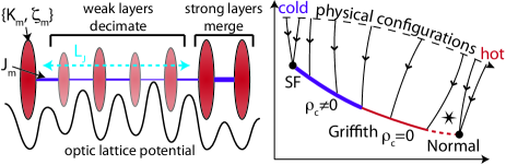
Figure 1: Left: Schematic diagram of the model: red ovals (purple bars) represent the superfluid layers (Josephson couplings) with size inversely proportional to vortex fugacity $\zeta_{m}$ (directly proportional to Josephson coupling $J_{m}$). The effects of the real space RG is to merge strong layers, and decimate weak layers. Emergent length-scale $L_{J}$ corresponds to the typical separation between strong layers.
Right: Schematic diagram of the RG flows showing the superfluid (SF) and normal fixed points along with the Griffiths fixed line. The black dashed line represents physical configurations, with points to the right corresponding to higher temperatures. The Griffiths fixed line is split into two segments, corresponding to the regimes with finite and zero c-axis superfluid response. The star indicates a possible unstable fixed point star .

The questions we raise are fast becoming important for experiments. Experiments on ultracold atoms observed both the BKT transition in large 2D “pancakes” produced by very deep 1D optical lattices Dalibard2006 , and Anderson localization of Bosons in 1D disordered optical lattices localization2008 ; Fallani2008 . The system we study here can be realized by constructing a stack of large 2D “pancakes” using a disordered 1D optical lattice and tests the effects of disorder near the 2D-3D crossover Affleck1996 ; Kasevich .

The model which we analyze and describe below consists of a set of coupled 2D superfluid layers. Each layer has a superfluid stiffness $K_{m}$, vortex fugacity (akin to vortex density per coherence length) $\zeta_{m}$, and Josephson coupling (to the next layer) $J_{m}$. $K_{m}$, $\zeta_{m}$ and $J_{m}$ are initially random and uncorrelated , see Fig. 1a. To analyze this model, we combine a Kosterlitz-Thouless like momentum space renormalization for the in-plane degrees of freedom KosterlitzThouless1973 ; Giamarchi2006 with a real-space RG (see, e.g., Fisher1994_95 ; AKPR2 ). In the real space-RG decimation, strongly coupled layers ($J_{m}\sim 1$) are merged, while vortex-ridden layers ($\zeta_{m}\sim 1$) are considered to be essentially normal and are perturbatively eliminated.

Before plunging into the analysis, let us summarize the phase diagram we find, see Fig. 1b and Table 1. At low temperatures the system forms a 3D superfluid. As the temperature is raised, a Griffiths phase appears; in it, the system breaks up into 2D superfluid puddles, each composed of one or several “pancakes”, with weak (power law distributed) inter-puddle tunneling. As the temperature is increased further, the c-axis superfluid response disappears altogether, while the system remains superfluid in the a- and b-directions, realizing a sliding phase. At yet higher temperatures, the in-plane superfluid response smoothly vanishes as the system becomes fully normal.

$T$	phase	$\rho_{ab}$	$\rho_{c}$	$J_{c,ab}$	$J_{c,c}$
high	Normal	zero	zero	zero	zero
	Griffith-Sliding	finite	zero	finite	zero
	Griffiths		finite
low	Superfluid	finite	finite	finite	finite

Table 1: Phase diagram indicating the properties of the various phases.

The Griffiths phase is perhaps the most surprising aspect of our results. At intermediate temperatures, the flow leads to a fixed line characterized by a stationary power-law distribution of inter-layer tunnelings, $J_{m}$, which are $P(J)\sim J^{\nu_{J}-1}$ (Fig. 1b). The appearance of these Griffiths phase power laws are a direct consequence of the disorder. Most layers have strong fluctuations, and turn insulating; Neighboring layer of either side, can still exchange bosons but with a smaller amplitude, e.g., $J_{\text{eff}}=J_{m-1}\cdot J_{m}$ if layer $m$ is eliminated. The elimination of all incoherent layers marks a first epoch in the RG flow, and upon its end the internally coherent layers are separated from each other by, on average, $L_{J}$ incoherent layers Fig. 1a. $L_{J}$ determines $\nu_{J}$: $\nu_{J}\sim\log[1/\bar{J}]/L_{J}$, with $\bar{J}$ the typical initial Josephson coupling. In the subsequent RG epoch, layers only merge, but $\nu_{J}$ remains unchanged.

The Griffiths phase can be separated into two regimes. A sliding regime with $\nu_{J}$ flowing to $\nu_{J}<1$ (as indicated in Fig. 1b), where there is no c-axis stiffness, and a Griffiths superfluid with a finite c-axis stiffness and $\nu_{J}>1$. Both regimes have a vanishingly small c-axis critical current. To wit, the critical current of $n$ layers is determined by the weakest effective tunneling between them. The expectation value for the longest run of weak layers is ${\cal R}_{n}\sim\log_{1/p_{\text{weak}}}\left[n(1-p_{\text{weak}})\right]$ Schilling1990 (with $p_{\text{weak}}$ the probability of a layer to be normal in the first epoch; $L_{J}=(1-p_{\text{weak}})^{-1}\gg 1$). The weakest link is thus $I_{c}\sim\left(\frac{n}{L_{J}}\right)^{L_{J}\log\overline{J}}$.

Model — Let us now describe the model and its analysis more precisely, before discussing more of its consequences and experimental implications. Following Ref. Giamarchi2006 , our model consists of a set of coupled $1+1$ dimensional (Euclidean) sine-Gordon models with partition function $Z=\text{Tr}\,\exp-\sum_{m}\left(S_{sG;m}+S_{J;m,m+1}\right)$ where

$$S_{sG;m} =\int dydx\big{[}K_{m}(\partial_{x}\theta_{m})^{2}+\frac{1}{K_{m}}(\partial_{x}\phi_{m})^{2}$$

$$\quad\quad-2i(\partial_{x}\phi_{m})(\partial_{y}\theta_{m})+\zeta_{m}\cos(2\phi_{m})\big{]},$$ (1)

$$S_{J;m,m+1} =\int dydx,J_{m}\cos(\theta_{m}-\theta_{m+1}).$$ (2)

$S_{sG;m}$ is the sine-Gordon action that describes the density waves and vortices in the $m$-th layer; $S_{J;m,m+1}$ is the $m$ to $m+1$ tunneling; $\theta_{m}(x,y)$ and $\phi_{m}(x,y)$ are the superfluid order-parameter phase variable and its conjugate, respectively ($[\theta_{m}(r),\partial_{x}\phi_{m^{\prime}}(r^{\prime})]=i\pi\delta(r-r^{\prime})\delta_{m,m^{\prime}}$). We define $J_{m}={\cal J}_{m}/T$, $K_{m}={\cal K}_{m}/T$, and $\zeta_{m}\sim\exp(-E_{\text{core},m}/T)$ as the reduced Josephson coupling, superfluid stiffness, and vortex fugacity at temperature $T$, where $E_{\text{core},m}$ is the vortex core energy. We note that to define the sine-Gordon model we must specify the short-distance cut-off scale. We choose a single cut-off $a$ for all layers, and work in the units in which $a=1$.

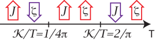
Figure 2: Schematic representation of relevance of $J$’s and $\zeta$’s as a function of temperature.

Renormalization Group — Our analysis relies on a combined c-axis real space and a-b momentum space RG. The momentum space transformation is given by :

$$\frac{dJ_{m}}{d\ell} =\!J_{m}\!\left[2\!-\!\frac{1}{4\pi K_{m}}\!-\!\frac{1}{4\pi K_{m+1}}\right]\!-\!\frac{\pi^{2}}{2}J_{m}\!\left(\zeta_{m}^{2}\!+\!\zeta_{m+1}^{2}\right),$$ (3)

$$\frac{d\zeta_{m}}{d\ell} =\zeta_{m}\left[2-\pi K_{m}\right]-\frac{1}{2}\pi^{2}\zeta_{m}(J_{m}^{2}+J_{m-1}^{2}),$$ (4)

$$\frac{dK_{m}}{d\ell} =-2\pi^{3}(K_{m}\zeta_{m})^{2}+\frac{\pi}{2}(J_{m}^{2}+J_{m-1}^{2}).$$ (5)

To lowest order in $\zeta_{m}$ and $J_{m}$, there is a range of superfluid stiffnesses $1/4\pi\lesssim K_{m}\lesssim 2/\pi$ in which both the vortex fugacity $\zeta_{m}$ and the Josephson coupling $J_{m}$ are relevant. The competition between the two gives rise to the Griffiths phase. Outside this range the system is either strongly superfluid (large $K_{m}$) or strongly insulating (small $K_{m}$), Fig. 2.

As the in-plane momentum shell RG proceeds, the real-space RG (RSRG) merges layers where $J_{m}$ rises to 1, or eliminates layers where vortex fugacity $\zeta_{m}$ reaches to 1. When a Josephson coupling becomes large, $J_{i}=1$, the relative phase $\Delta\theta=\theta_{i+1}-\theta_{i}$ of the two neighboring layers becomes locked and the two layers merge into a single super-layer having $K_{\text{eff}}=K_{i}+K_{i+1}$ and $\zeta_{\text{eff}}=\zeta_{i}\cdot\zeta_{i+1}$. Similarly, if one of the vortex fugacities becomes large, $\zeta_{i}=1$, then the conjugate field $\phi_{i}$ in that layer becomes locked and vortices proliferate. Upon integrating out the incoherent layer, we find that it suppresses tunneling across it to $J_{\text{eff}}=J_{i-1}\cdot J_{i}$. These RG rules make it convenient to parametrize $J$ and $\zeta$ in terms of their logs $j=\log(1/J),\,z=\log(1/\zeta)$ which yields:

$$j_{\text{eff}} =j_{i-1}+j_{i} z_{\text{eff}} =z_{i-1}+z_{i}.$$ (6)

Next, instead of a numerical analysis of the RG outlined above (which we will fully pursue in a separate work  LongPaper ), let us use the RG procedure to derive the approximate flow of the distribution functions for $K$, $j$,  and $z$, and their universal aspects. First, note that the RSRG layer merging step leads to strong correlations of $K$’s and $\zeta$’s. Therefore, alongside the distribution $P_{j}$ for $j_{m}$’s, we use the joint probability distribution $Q_{K}^{z}$ for $z_{m}$’s and $K_{m}$’s. The fRG equations resulting from Eqs. (5, 6) and the:

$$\frac{dP_{j}}{d\ell} =I_{1}\,\partial_{j}P_{j}-\int dK_{1}Q_{K_{1}}^{0}\{2-\pi K_{1}\}P_{j}$$

$$\!\!\!+\!\int\!\!dK_{1}Q_{K_{1}}^{0}\{2\!-\!\pi K_{1}\}\int\!dj^{\prime}P_{j^{\prime}}P_{j-j^{\prime}}+I_{1}P_{0}P_{j},$$ (7)

$$\frac{dQ_{K}^{z}}{d\ell} =\!(2\!-\!\pi K)\partial_{z}Q_{K}^{z}\!-\!\!\int\!\!d1\,Q_{1}\!\left(\!2\!-\!\frac{1}{4\pi K_{1}}\!-\!\frac{1}{4\pi K}\!\right)\!Q_{K}^{z}\!P_{0}$$

$$+\int d1\,Q_{1}Q_{K-K_{1}}^{z-z_{1}}\left(2-\frac{1}{4\pi K_{1}}-\frac{1}{4\pi(K-K_{1})}\right)P_{0}$$

$$+\int dK_{1}\,Q_{K_{1}}^{0}\{2-\pi K_{1}\}Q_{K}^{z},$$ (8)

where $I_{1}=\int d1\,d2\,Q_{1}Q_{2}\left(2-\frac{1}{4\pi K_{1}}-\frac{1}{4\pi K_{2}}\right)$, $\{g\}$ stands for $g\Theta(g)$ with $\Theta$ being the step function; $d1$ and $Q_{1}$ are shorthand for $dK_{1}dz_{1}$ and $Q_{K_{1}}^{z_{1}}$ where it is unambiguous. Briefly, the first terms of Eqs. (7) and (8) correspond to the action of the linear in $J_{m}$ and $\zeta_{m}$ terms of the momentum space RG Eqs. (3) and (4). The remaining terms correspond to the action of the real space RG, where we keep in mind the fact that the distributions must be normalized. The normalization is accomplished by rescaling the distributions $P_{j}$ and $Q_{K}^{z}$ whenever layers are removed from the system. The fRG equations must be supplemented by absorbing wall boundary conditions $Q_{K}^{0^{-}}=0$ and $P_{0^{-}}=0$ which remove the small $z$’s and $j$’s (large $\zeta$’s and $J$’s) from the distributions when layers are decimated or merged. In order to compute physical observables we also keep track of $n(\ell)$, the number of surviving layers at RG scale $\ell$:

$$\frac{dn}{d\ell}=-n\left(I_{1}P_{0}+\int dK_{1}\,\{2-\pi K_{1}\}Q_{K_{1}}^{0}\right).$$ (9)

Note that the structure of the fRG and of the resulting flows are similar to those in Ref. Vojta2008 ; Rosenow for the damped transverse field Ising model .

To study the evolution of $P_{j}(l)$ and $Q_{K}^{z}(l)$ under coarse graining, we numerically integrate Eqs. (7) and (8). To parametrize the initial distributions at temperature $T$ (and length scale $a$), we choose smooth functions with the following bounds: $0.04<TJ<0.11$, $1.0<TK<1.5$, and $e^{-1.6\pi\cdot 1.5/T}<\zeta<e^{-1.6\pi\cdot 1.0/T}$ .

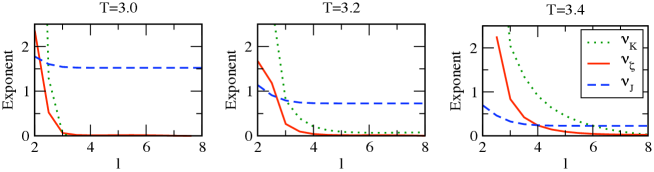
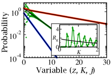
Figure 3: Left three panels: flow of exponents $\nu_{\zeta}$, $\nu_{K}$, and $\nu_{J}$ under the action of the coarse graining transformation for three different initial distributions corresponding to temperatures $T=3.0$, $3.2$, and $3.4$. $l\sim 3$ separates the first epoch, in which all three exponents flow from the second epoch in which only $\nu_{\zeta}$ and $\nu_{K}$ flow. The asymptotic value of $\nu_{J}$ at long length-scales indicates that $T=3.0$ corresponds to a Griffiths superfluid, while $T=3.2$ and $3.4$ correspond to Griffith insulator.
Right panel: semi-log plot of typical distributions (from top to bottom) $Q[z]$, $R[K]$, and $P[j]$, obtained by solving Eqs. (7) and (8) numerically and the corresponding exponential fits (black solid lines) that are used to obtain the values of exponents $\nu_{\zeta}$, $\nu_{K}$, and $\nu_{J}$. The inset depicts the distribution $R[K]$ on a linear-linear plot, the oscillations arise from additions of $K$ values when layers merge.

Results — A numerical analysis of the flows reveals three phases: (1) superfluid phase – all layers merge, (2) Griffiths phase – power law distributions $P_{J}\sim J^{\nu_{J}-1}$ with a finite $\nu_{J}$, (3) insulating phase – all layers decimate. Phases (1) and (3) correspond to the usual superfluid and insulating fixed points, the Griffiths phase, regime (2), corresponds to a new fixed line that is induced by disorder star .

Within the Griffiths phase, the flow of $P_{j}$ and $Q_{K}^{z}$ distributions occurs in two epochs, as depicted in Fig. 3. In the first epoch both mergers and layer eliminations take place, which quickly results in the formation of power law distributions with flow of all three exponents. However, as mergers lead to ever increasing $K$’s while eliminations do not, the flow eventually exhausts all weak layers by eliminating them, and only the strongly superfluid layers remain. In the second epoch, only $J$’s (but not $\zeta$’s) remain relevant as all the surviving $K$’s exceed $2/\pi$, so while layers continue to merge, no eliminations occur. As a result, $\nu_{J}$ saturates while both $\nu_{K}$ and $\nu_{\zeta}$ decay to zero exponentially in the fRG flow parameter $\nu_{K}\sim\nu_{\zeta}\sim e^{-2\nu_{J}\ell}$. We see, therefore, that the Griffiths fixed line corresponds to a line of fixed $\nu_{J}$’s with $\nu_{K}\rightarrow 0$ and $\nu_{\zeta}\rightarrow 0$.

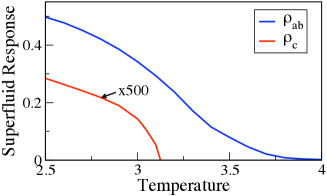
Figure 4: The in-plane ($\rho_{ab}$) and out-of-plane ($\rho_{c}$) stiffness as a functions of temperature evaluated using value of RG parameter is sufficiently large ($l=10$) so that the flows are saturated. While $\rho_{ab}$ undergoes a smeared phase transitions, as indicated by the absence of a critical point with power law behavior, $\rho_{c}$ undergoes a continuous phase transition at $T\sim 3.1$.

Both the in-plane $\rho_{ab}$ and the out-of-plane $\rho_{c}$ superfluid responses have a very peculiar behavior within the Griffith phase, and can be used to as probes. The mean values of the superfluid responses may be obtained from the distributions via

$$\rho_{ab} =n\int dz\,dKKQ_{K}^{z},$$ (10)

$$\rho_{c} =\chi(l)+e^{-2l}\left(n\int dje^{j}P_{j}\right)^{-1},$$ (11)

where, $n$, which is given by Eq. (9), is the fraction of surviving layers and is needed to normalize the response to the scale of the original system. $\chi(l)$ obeys

$$\partial_{l}\chi(l) =nP_{0}e^{2l}I_{1} \chi(0) =0,$$ (12)

and accounts for stiffness within the superfluid “puddles”. As $\rho_{c}$ depends on the area, we include the factor of $e^{-2l}$ in Eq. 11 to account for its renormalization. We plot $\rho_{ab}$ and $\rho_{c}$ as a function of $T$ near saturation (at large value of the RG parameter $\ell$) in Fig. 4. The smearing of the phase transition is reflected in $\rho_{ab}$ decreasing smoothly, as the temperature is increased, until reaching zero at the end of the Griffiths fixed line (without following any power law). On the other hand, $\rho_{c}$ decreases much faster, becoming zero within the Griffith phase at the point where $\lim_{\ell\rightarrow\infty}\nu_{J}(\ell)$ becomes smaller than unity. The disappearance of $\rho_{c}$ signals the onset of the elusive sliding subphase of the Griffith phase, see Table 1.

Experimental probes — In our analysis we found that disorder smears the superfluid-to-normal phase transition. This could be probed experimentally in the ultra-cold atom setting. The superfluid response as well as the critical current could be measured by jolting the confined gas (e.g. quickly displacing the trap potential) and looking at the decay of the center of mass oscillations McKay2008 . Alternatively, one could look at correlations by removing the optical lattice and the trap potentials and allowing the atoms from the various pancakes to expand and interfere. The key signature of the Griffiths phase, in interference experiments, is very strong shot noise which results from the interference of several weakly coupled superfluid droplets LongPaper . Alternatively, in the mesoscopic setting, the Griffiths phase could appear in artificially grown structures composed of alternating layers of superconducting and insulating films of varying thicknesses. In this setting the anisotropy superfluid responses and critical currents could be measured directly.

Conclusions — In this manuscript we investigated the effects of reduced dimensionality disorder on a phase transition at a higher dimensionality. We focus on a model that we believe is relevant to experiments in ultra-cold gases in optical lattices, and mesoscopic systems such as stacked superconducting films. Naively, one would expect that, the strong disorder picture of Ref. Fisher1994_95 should be in effect. However, the classification scheme of Ref. Vojta2006 indicates that the existence of the BKT transition for a single 2D layer boosts the importance of disorder in our system, resulting in the stronger effect of the smearing of the phase transition. Using a functional renormalization group scheme that we develop, we show that this is indeed the case. Further, we show that in the transition region the system becomes essentially two dimensional. We find that the reduction of dimensionality is reflected in the strong anisotropy of physical observables like critical current and superfluid response.

As we were finalizing this manuscript, we became aware of a complementary investigation of the random superfluid stack from a scaling perspective by Vojta and Narayanan, which is consistent with our findings.

Acknowledgements It is our pleasure to thank Michael Lawler, Subir Sachdev, and Bryan Clark for insightful discussions. DP and ED acknowledge support from DARPA, CUA, and NSF Grant No. DMR-07-05472. GR gratefully acknowledges support from the Packard Foundation, the Sloan Foundation, and the Cottrell Scholars program.

References

- (1) P. W. Anderson, Phys. Rev. 109, 1492 (1958).
- (2) D. S. Fisher, Phys. Rev. B 50, 3799 (1994); D. S. Fisher, Phys. Rev. B 51, 6411 (1995).
- (3) J. Billy, V. Josse, Z. Zuo, A. Bernard, B. Hambrecht, P. Lugan, D. Clement, L. Sanchez-Palencia, P. Bouyer, and A. Aspect, Nature 453, 891 (2008); G. Roati, C. D’Errico, L. Fallani, M. Fattori, C. Fort, M. Zaccanti, G. Modugno, M. Modugno, and M. Inguscio, Nature 453, 895 (2008).
- (4) E. Altman, Y. Kafri, A. Polkovnikov, and G. Refael, Phys. Rev. Lett. 93, 150402 (2004).
- (5) E. Altman, Y. Kafri, A. Polkovnikov, and G. Refael, Phys. Rev. Lett. 100, 170402 (2008).
- (6) V. L. Berezinskii, Sov, Phys. JETP 34, 610 (1972).
- (7) J. M. Kosterlitz and D. J. Thouless, J. Phys. C: Solid State Phys. 6, 1181 (1973).
- (8) T. Vojta, J. Phys. A: Math. Gen. 39, R143 (2006).
- (9) J. A. Hoyos and T. Vojta, Phys. Rev. Lett. 100, 240601 (2008); T. Vojta, C. Kotabage, and J. A. Hoyos, Phys. Rev. B 79, 024401 (2009).
- (10) C. S. O’Hern, T. C. Lubensky, and J. Toner, Phys. Rev. Lett. 83, 2745 (1999).
- (11) Z. Hadzibabic, P. Kruger, M. Cheneau, B. Battelier, and J. Dalibard, Nature 441, 1118 (2006).
- (12) See e.g. the review L. Fallani, C. Fort, and M. Inguscio arXiv:0804.2888 and references therein.
- (13) I. Affleck and B. Halperin, J. Phys A: Math. Gen. 29. 2627 (1996).
- (14) S. Burger, F. S. Cataliotti, C. Fort, P. Maddaloni, F. Minardi and M. Inguscio, Europhys. Lett. 57, 1 (2002); W. Li, H.-C. Chien, and M. Kasevich, private communications.
- (15) M. A. Cazalilla, A. F. Ho, and T. Giamarchi, New J. Phys. 8, 158 (2006).
- (16) M. F. Schilling, The College Math. J. 21, 196 (1990).
- (17) B. K. Clark, D. Pekker, G. Refael, E. Demler, in preparation.
- (18) A. Del Maestro, B. Rosenow, M. Mueller, and S. Sachdev, Phys. Rev. Lett. 101, 035701 (2008).
- (19) D. McKay, M. White, M. Pasienski, and B. DeMarco, Nature 453, 76 (2008); M. Pasienski, D. McKay, M. White, and B. DeMarco, arXiv:0908.1182.
- (20) We suspect that there may be an additional unstable fixed point, indicated by the star in Fig. 1b. However, due to the complexity of the fRG equations, we were unable to find it or rule it out.