Two-step Emergence of the Magnetic Flux Sheet
from the Solar Convection Zone

Abstract

We perform two-dimensional MHD simulations of the flux emergence from the solar convection zone to the corona. The flux sheet is initially located moderately deep in the adiabatically stratified convection zone ($-20,000\ {\rm km}$) and is perturbed to trigger the Parker instability. The flux rises through the solar interior due to the magnetic buoyancy, but suffers a gradual deceleration and a flattening in the middle of the way to the surface since the plasma piled on the emerging loop cannot pass through the convectively stable photosphere. As the magnetic pressure gradient enhances, the flux becomes locally unstable to the Parker instability so that the further evolution to the corona occurs. The second-step nonlinear emergence is well described by the expansion law by Shibata et al. (1989). To investigate the condition for this ‘two-step emergence’ model, we vary the initial field strength and the total flux. When the initial field is too strong, the flux exhibits the emergence to the corona without a deceleration at the surface and reveals an unrealistically strong flux density at each footpoint of the coronal loop, while the flux fragments within the convection zone or cannot pass through the surface when the initial field is too weak. The condition for the ‘two-step emergence’ is found to be $10^{21}-10^{22}\ {\rm Mx}$ with $10^{4}\ {\rm G}$ at $z=-20,000\ {\rm km}$. We have some discussions in connection with the recent observations and the results of the thin-flux-tube model.

1 Introduction

Solar active regions are generally thought to be the consequence of the flux emergence, i.e., dynamo-generated magnetic fluxes risen from the deep convection zone due to the magnetic buoyancy force (Parker, 1955). Observations indicate that the flux tube should be in a coherent form and strong enough so as not to be disintegrated by the turbulent motion during its emergence through the convection zone. For generating such a strong flux, the sub-adiabatically stratified overshoot region at the bottom of the convection zone has been suggested to be the suitable place (Parker, 1975). Therefore, a flux emergence should be understood as a whole process from the base of the convective layer to the upper atmosphere through the surface.

In last two decades, various series of numerical experiments have been carried out to investigate the physics of the flux emergence. For the local evolution above the surface, the pioneering work was done by Shibata et al. (1989), who performed two-dimensional (2D) magnetohydrodynamic (MHD) simulations of flux emergence through the undular mode of magnetic buoyancy instability ($\mbox{\boldmath$k$}\parallel\mbox{\boldmath$B$}$, where $k$ and $B$ denote the wavenumber and the initial magnetic field vector, respectively; the Parker instability) to reproduce some dynamical features such as the rise motion of an arch filament system and downflows along the magnetic field lines. Since then, the evolution of an emerging flux and the interaction with pre-existing coronal fields have been studied by 2D and 3D simulations (Nozawa et al., 1992; Matsumoto et al., 1993; Yokoyama & Shibata, 1995, 1996; Fan, 2001b; Cheung et al., 2008). Nozawa et al. (1992) performed the emergence from the convectively unstable solar interior (the convective-Parker instability), while Yokoyama & Shibata (1995, 1996) studied the reconnection between the expanding loop and the pre-existing fields in the corona and the subsequent formation of X-ray jets. Three-dimensional calculations by Matsumoto et al. (1993) were performed for the studies of the interchange ($\mbox{\boldmath$k$}\perp\mbox{\boldmath$B$}$) and quasi-interchange ($\mbox{\boldmath$k$}\parallel\mbox{\boldmath$B$}$ with $kH_{\rm ph}\ll 1$, where $H_{\rm ph}$ is the photospheric pressure scale height) mode instabilities. Fan (2001b) compared her 3D simulation results with observed features of newly emerged active regions. Cheung et al. (2008) found that the numerical modeling of emerging flux regions by 3D radiative MHD simulations exhibits photospheric characteristics that are comparable with the observations from the Hinode/Solar Optical Telescope (SOT). These simulations assumed that the initial flux is embedded just below the photosphere ($\gtrsim-2000\ {\rm km}$) a priori as a horizontal sheet or a twisted tube. It is because their experiments mainly aimed to clarify the local behaviors in the solar atmosphere. Such an initial structure, however, is not obvious since the initial form depends on its history of pushing through the convection zone. Therefore, a numerical experiment including the evolution from a substantial depth has been needed.

The simulations focusing on the flux emergence within the relatively deep solar interior have been done by using the thin-flux-tube approximation (Spruit, 1981; D’Silva & Choudhuri, 1993; Caligari et al., 1995). One of the most important conclusions obtained from the various thin-flux-tube simulations is that rising tubes with small magnetic flux (below 10²¹ Mx for 10⁴ G at the base) cannot reach the photosphere because the apices of the loops loose magnetic fields and subsequently ‘explode’ (Moreno-Insertis et al., 1995). By assuming the anelastic approximation (Gough, 1969; Lantz & Fan, 1999), Fan (2001a) computed the evolution of the 3D undulatory instability of the horizontal magnetic flux layer, which formed arch-like magnetic tubes with downflows from their apices to the troughs. Note that both types of approximations (thin-flux-tube and anelastic) are not applicable in the upper convection zone ($\gtrsim-30\ {\rm Mm}$) where the diameter of the flux tube exceeds the local pressure scale height and the flow velocity becomes close to the sound speed.

Abbett & Fisher (2003) calculated a flux emergence by connecting the anelastic MHD convective layer and the fully compressible MHD solar atmosphere from the photosphere to the low corona. However, their full MHD atmosphere did not include the upper convection zone. To investigate the detailed behavior of the emerging flux from the convection zone to the atmosphere, we have to deal with the full MHD numerical box including the convective layer, the photosphere/chromosphere, and the corona.

The dynamical behavior of an emerging flux including both the interior and the upper atmosphere is not yet clear, but is thought to obey the following picture, which we name ‘two-step emergence’ model (cf. Matsumoto et al., 1993; Magara, 2001). Magnetic fluxes emerged from the bottom of the convection zone are depressed and decelerated by the sub-adiabatic photosphere and extended horizontally around the photosphere/chromosphere. Meanwhile, fluxes are still transported from below to enhance the magnetic pressure gradient. Finally, the fluxes above the photosphere become unstable to the magnetic buoyancy instability so that the further evolution into the corona occurs. By the development of supercomputers, full MHD simulations in the convection zone without approximations have come to be realizable. The purpose of this work is to investigate the ‘two-step emergence’ model numerically.

Several experiments have confirmed this ‘two-step’ model. Magara (2001) studied the emergence of the magnetic flux tube from the convection zone by means of 2.5-dimensional MHD simulations focused on the cross section of the tube. He found the deceleration of the rising flux tube due to the convectively stable photosphere and the subsequent horizontal outflow. Archontis et al. (2004) performed 3D simulations using the criterion by Acheson (1979) to analyze the magnetic buoyancy instability within the photosphere/chromosphere, while Murray et al. (2006) did parameter studies of the dependence of the initial magnetic field strength of the tube and its twist, finding that the tube evolves in the self-similar way when varying the field strength and that the magnetic buoyancy instability and the second-step evolution do not occur when the field is too weak. In these studies, the initial flux tubes are located in the uppermost convective region at some 1000 km depth. Recently, Solar Optical Telescope (SOT) aboard the Hinode satellite (e.g. Tsuneta et al., 2008) observed small-scale magnetic flux emergence. Thanks to high-resolution and high-cadence multi-wavelength observations, Otsuji et al. (2010) found the deceleration of the apex of the arch filament system in the chromosphere, which can be the possible evidence of the two-step model.

In this study, we perform two-dimensional fully compressible MHD simulations to investigate the dynamical evolution from the adiabatically stratified convective layer into the corona through the isothermal (strongly sub-adiabatic, i.e., convectively stable) photosphere/chromosphere. We set the initial magnetic flux sheet in the moderately deep convection zone at 20 Mm depth, not at the bottom of the solar interior, because the emergence from the base is beyond the computation ability. The numerical results reproduce the two-step model well. However, the picture of the two-step emergence is much far from the previous studies (e.g. Magara, 2001; Archontis et al., 2004; Murray et al., 2006). The location of the initial flux is so deep that the typical wavelengths of the Parker instability ($10-20$ times the local pressure scale height) are different between the primary and the secondary emergence; the first-step evolution occurs at $z=-20\ {\rm Mm}$ and its typical wavelength is about $100\ {\rm Mm}$, while, at the photosphere, the second-step emergence has its wavelength of the order of a few $1000\ {\rm km}$. We also discuss the dependence of the flux sheet’s behavior (‘two-step emergence’, ‘direct emergence’ or ‘failed emergence’) on its magnetic field strength and amount of fluxes through the parameter survey.

The numerical setup and the assumed conditions used in this study are presented in Section 2. We show the typical case of the ‘two-step emergence’ in Section 3, while Section 4 gives the results of the parameter survey and make some discussions with preceding studies and recent observations. Finally, in Section 5, we summarize the study.

2 Numerical Model

2.1 Assumptions and Basic Equations

We consider an isolated magnetic flux sheet located in a convectively marginally stable gas layer in a two-dimensional Cartesian coordinate system ($x,\,z$), where $z$-direction is antiparallel to the gravitational acceleration. We solve adiabatic two-dimensional ($\partial/\partial y=0,\,B_{y}=0,\,V_{y}=0$) magnetohydrodynamic (MHD) equations. The basic equations are as follows;

$$\frac{\partial\rho}{\partial t}+\mbox{\boldmath$\nabla$}\cdot(\rho\mbox{\boldmath$V$})=0\ ,$$ (1)

$$\frac{\partial(\rho\mbox{\boldmath$V$})}{\partial t}+\mbox{\boldmath$\nabla$}\cdot\left(\rho\mbox{\boldmath$VV$}+p\mbox{\boldmath$I$}-\frac{\mbox{\boldmath$BB$}}{4\pi}+\frac{\mbox{\boldmath$B$}^{2}}{8\pi}\mbox{\boldmath$I$}\right)-\rho\mbox{\boldmath$g$}=0\ ,$$ (2)

$$\frac{\partial\mbox{\boldmath$B$}}{\partial t}=\mbox{\boldmath$\nabla$}\times(\mbox{\boldmath$V$}\times\mbox{\boldmath$B$})\ ,$$ (3)

$$\frac{\partial}{\partial t}\left(\rho U+\frac{1}{2}\rho\mbox{\boldmath$V$}^{2}+\frac{\mbox{\boldmath$B$}^{2}}{8\pi}\right)+\mbox{\boldmath$\nabla$}\cdot\left[(\rho U+p+\frac{1}{2}\rho\mbox{\boldmath$V$}^{2})\mbox{\boldmath$V$}+\frac{c}{4\pi}\mbox{\boldmath$E$}\times\mbox{\boldmath$B$}\right]-\rho\mbox{\boldmath$g$}\cdot\mbox{\boldmath$V$}=0\ ,$$ (4)

and

$$U=\frac{1}{\gamma-1}\frac{p}{\rho}\ ,$$ (5)

$$\mbox{\boldmath$E$}=-\frac{1}{c}\mbox{\boldmath$V$}\times\mbox{\boldmath$B$}\ ,$$ (6)

where $U$ is the internal energy per unit mass, $I$ is the unit tensor, $\mbox{\boldmath$g$}=(0,0,-g_{0})$ ($g_{0}$ is constant and its value is given below) is the gravitational acceleration, and other symbols have their usual meanings. We assume a ratio of specific heats, $\gamma$, of 5/3.

2.2 Initial Conditions

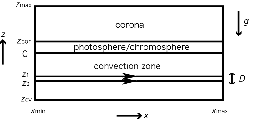
Figure 1: 1 Schematic depiction of the initial set-up. 1 One-dimensional ($z$-)distributions of the initial density (solid line), pressure (dotted line), temperature (dashed line), and magnetic field strength (dashed-dotted line).

The initial magnetostatic gas layer is composed of three regions: hot and cold isothermal layers in upper and middle regions represent a very simplified model of the solar corona and photosphere/chromosphere, and a non-isothermal layer in the lower region models the convection zone (see Fig. 1). We take $z=0$ to be the base height of the photosphere. The units of length, velocity, time, and density in the simulations are $H_{0}$, $C_{s0}$, $H_{0}/C_{s0}\equiv\tau_{0}$, and $\rho_{0}$, respectively, where $H_{0}=k_{\rm B}T_{0}/(mg_{0})$ is the pressure scale height ($k_{\rm B}$ is Boltzmann constant and $m$ is mean molecular mass), $C_{s0}$ the sound speed, and $\rho_{0}$ the density at $z=0$ in the photosphere. The gas pressure, temperature, and magnetic field strength are normalized by the combinations of the units above, i.e., $p_{0}=\rho_{0}C_{s0}^{2}$, $T_{0}=mC_{s0}/(\gamma k_{\rm B})$, and $B_{0}=(\rho_{0}C_{s0}^{2})^{1/2}$, respectively. The gravity is given as $g_{0}=C_{s0}^{2}/(\gamma H_{0})$ by definition. For the comparison of numerical results with observations, we use $H_{0}=200\ {\rm km}$, $C_{s0}=8\ {\rm km\,s}^{-1}$, $\tau_{0}=H_{0}/C_{s0}=25\ {\rm s}$, and $\rho_{0}=1.4\times 10^{-7}\ {\rm g\ cm}^{-3}$, which are typical values for the solar photosphere and chromosphere. Then, $p_{0}=9.0\times 10^{4}\ {\rm dyn\ cm}^{-2}$, $T_{0}=4000\ {\rm K}$, and $B_{0}=300\,{\rm G}$.

The initial temperature distribution of the photosphere/chromosphere and the corona $(z\geq 0)$ is assumed to be

$$T(z)=T_{\rm ph}+(T_{\rm cor}-T_{\rm ph})\left\{\tanh{[(z-z_{\rm cor})/w_{\rm tr}]+1}\right\}/2\ ,$$ (7)

where $T_{\rm cor}$ and $T_{\rm ph}$ are the respective temperatures in the corona and in the photosphere/chromosphere, $z_{\rm cor}$ is the height of the base of the corona, and $w_{\rm tr}$ is the temperature scale height of the transition region. We take $T_{\rm cor}=100T_{0}$, $T_{\rm ph}=T_{0}$, $z_{\rm cor}=10H_{0}$, and $w_{\rm tr}=0.5H_{0}$. As for the initial temperature distribution in the convective layer ($z\leq 0$), we assume

$$T(z)=T_{\rm ph}-\alpha z\left|\frac{dT}{dz}\right|_{\rm ad}\ ,$$ (8)

where

$$\left|\frac{dT}{dz}\right|_{\rm ad}=\frac{\gamma-1}{\gamma}\frac{mg_{0}}{k_{\rm B}}$$ (9)

is the adiabatic temperature gradient, and $\alpha$ is a parameter of the temperature gradient of the convection zone. In our calculations, $\alpha$ is set to be unity, i.e., the initial temperature distribution in the convection zone is adiabatic.

The magnetic field is initially horizontal, $\mbox{\boldmath$B$}=(B_{x}(z),0,0)$, and is embedded in the convection zone. The distribution of magnetic field strength is given by

$$B_{x}(z)=[8\pi p(z)/\beta(z)]^{1/2}\ ,$$ (10)

where

$$\beta(z)=\beta_{\ast}/f(z)\ ,$$ (11)

and

$$f(z)=\frac{1}{4}\left[\tanh{\left(\frac{z-z_{0}}{w_{0}}\right)}+1\right]\left[-\tanh{\left(\frac{z-z_{1}}{w_{1}}\right)}+1\right]\ .$$ (12)

Here $\beta_{\ast}$ is the ratio of gas pressure to magnetic pressure at the center of the magnetic flux sheet, and $z_{0}$ and $z_{1}=z_{0}+D$ are the heights of the lower and upper boundaries of the flux sheet, where $D$ is the vertical thickness of the sheet. We use $z_{0}=-100H_{0}\simeq-20,000\,{\rm km}$. In all of our calculations, $w_{0}$ and $w_{1}$ are set to be $0.5H_{0}$. We take $\beta_{\ast}=160$ and $D=5H_{0}\simeq 1000\,{\rm km}$ for case 1 (the typical model), so as the initial magnetic field strength $B_{x}$ to be $10^{4}\,{\rm G}$ and the total magnetic flux $\Phi$ to be $10^{21}\,{\rm Mx}$. To calculate the total magnetic flux, we regard the initial flux sheet as a rectangular prism with a base $D$ (in $z$ direction) by $10D$ (in $y$ direction).

On the basis of the initial plasma $\beta$ distribution mentioned above, the initial density and pressure distribution are calculated numerically by using the equation of static pressure balance:

$$\frac{d}{dz}\left[p+\frac{B_{x}^{2}}{8\pi}\right]+\rho g_{0}=0\ .$$ (13)

The initial temperature, density, pressure, and magnetic field strength distributions for the typical case are shown in Fig. 1.

In order to trigger the Parker instability Parker (1966) in the convection zone, small density perturbations of the form

$$\delta\rho=Af(z)\rho(x,z)\cos{(2\pi x/\lambda)}$$ (14)

are initially reduced from the magnetic flux sheet ($z_{0}\leq z\leq z_{1}$) within the finite horizontal domain ($-3\lambda/4<x<3\lambda/4$), where $\lambda(=400H_{0})$ is the perturbation wavelength, and $A(=0.01)$ is the maximum value of the initial density reduction. The definition of $f(z)$ is given in equation (12).

2.3 Boundary Conditions and Numerical Procedures

The domain of the simulation box is $(x_{\rm min}<x<x_{\rm max})$ and $(z_{\rm min}<z<z_{\rm max})$, where $x_{\rm min}=-400H_{0}$, $x_{\rm max}=400H_{0}$, $z_{\rm min}=-200H_{0}$, and $z_{\rm max}=200H_{0}$, i.e., the total size of the box is $160\ {\rm Mm}\times 80\ {\rm Mm}$. This is much larger than those of the calculations focusing on the emergence from the uppermost convection zone to the corona (e.g. Shibata et al., 1989, etc.). Periodic boundaries are assumed for $x=x_{\rm min}$ and $x=x_{\rm max}$, symmetric boundaries for $z=z_{\rm min}$ and $z=z_{\rm max}$. A damping zone is attached near the top boundary to reduce the effects of reflected waves.

To solve the equations numerically, we use the modified Lax-Wendroff scheme. The code is a part of the numerical package CANS (Coordinated Astronomical Numerical Software) maintained by Yokoyama et al . For the typical model (case 1), the total number of grid points is $(N_{x}\times N_{z})=(1536\times 1920)$, and the mesh sizes are $\Delta x=0.52H_{0}$ and $\Delta z=0.21H_{0}$, both of which are uniform. For comparison, we perform other simulations with different values of the parameters. We vary the values of the initial magnetic field strength $B_{x}$ and of the total magnetic flux $\Phi$ of the emerging flux sheet by adjusting $\beta_{\ast}$ and $D$. In these calculations we set the total number of grid points $(N_{x}\times N_{z})=(1024\times 1280)$, and the uniform mesh sizes $\Delta x=0.78H_{0}$ and $\Delta z=0.31H_{0}$. The cases we examine are summarized in Table 1.

3 General Evolution

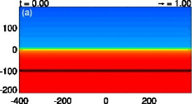
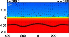
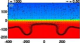
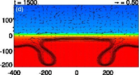
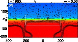
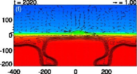
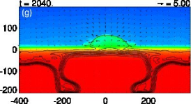
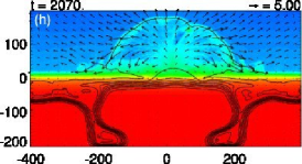
Figure 2: Time-evolution of the ‘two-step emergence’ for case 1 (typical model). 2 $t/\tau_{0}=0$; 2 $t/\tau_{0}=500$; 2 $t/\tau_{0}=1000$; 2 $t/\tau_{0}=1500$; 2 $t/\tau_{0}=1960$; 2 $t/\tau_{0}=2020$; 2 $t/\tau_{0}=2040$; 2 $t/\tau_{0}=2070$. Logarithmic density profiles ($\log_{10}{(\rho/\rho_{0})}$) are indicated by color contour, while magnetic field lines and velocity vectors are overplotted with black lines and arrows. The white box at $t/\tau_{0}=1960$ shows the area we analyze the Parker instability (see Fig. 8). This figure is also available as an avi animation in the electronic edition of the Astrophysical Journal.

In this section we show the numerical results of the typical case (case 1: $B_{x}=10^{4}{\rm\,G}$ and $\Phi=10^{21}{\rm\,Mx}$); the results display the ‘two-step emergence’. Figure 2 illustrates the development of the density profile with magnetic field lines and velocity vectors, while Figure 3 indicates the height of the apex of the magnetic field $z_{\rm apex}$ and its rise velocity $V_{z{\rm apex}}$. The time evolution can be divided into four stages according to the rise velocity at the apex of the emerging field. In the first stage ($0<t/\tau_{0}<700$), the magnetic flux begins an emergence in the convection zone due to the Parker instability driven by the magnetic buoyancy (Fig. 2). The rise velocity increases continuously in this stage (Fig. 3). The second stage ($700<t/\tau_{0}<1900$) is characterized by a gradual deceleration (Fig. 3) because the arch-like emerging field becomes deformed to horizontal so that the mass on the apex can no longer fall down along the field lines, and thus continues to pile up on the horizontal field. As a consequence, the emerging flux stretches around the solar surface (Figs. 2 and 2). In the third stage ($1900<t/\tau_{0}<2000$), the top part of the emerging magnetic flux almost stops at the surface while fluxes are still emerging from below, that is, the magnetic pressure gradient on the upper boundary of the flux sheet continues to enhance. When the magnetic pressure gradient gets steepened enough, the Parker instability sets in and drives the further evolution into the upper atmosphere (Figs. 2 and 2). In the final, fourth stage ($t/\tau_{0}>2000$), the magnetic flux evolves to the corona due to magnetic pressure, which is consistent with the results of classical calculations (e.g. Shibata et al., 1989) (Figs. 2 and 2). In the following, we will discuss each stage in more detail, and examine the dynamical structure of the expanding loop and the related forces acting on the magnetic field.

3.1 First Stage ($0<t/\tau_{0}<700$)

The initial sinusoidal perturbation in the flux sheet triggers the Parker instability so that the flux sheet begins to rise through the solar convection zone by magnetic buoyancy (Fig. 2). In this phase, the rise speed enhances continuously as the flux sheet emerges. The rising flux becomes arch-like shape owing to the stronger buoyancy of the loop center. The evacuation in the apex by the downflow along the field lines due to gravity leads to the acceleration of the loop until reaching the local Alfv$\acute{\rm e}$n speed ($C_{\rm A}=B/\sqrt{4\pi\rho}$). Figure 4 is a close-up view of the evolution between $t/\tau_{0}=400$ and $t/\tau_{0}=600$ of Figure 3, where a dashed line indicates the rise velocity of the apex, while the local Alfv$\acute{\rm e}$n speed is represented by a solid line. This figure shows that the rise velocity increases so as to get close to the local Alfv$\acute{\rm e}$n speed.

3.2 Second Stage ($700<t/\tau_{0}<1900$)

At around $t/\tau_{0}=700$, the rise velocity changes from acceleration to deceleration (Fig. 3), and at $t/\tau_{0}=1000$, both legs of the loop become vertical (Fig. 2). The central part of the emerging loop flattens and expands horizontally along the surface. Drained gas from the apex flows down along the field lines to each trough, so that the both troughs sink into the deep convection zone.

In this stage, the rise motion turns into the deceleration as seen from Figure 3. Magara (2001) found that the tube reduces its rise speed and becomes flattened since the rise motion cannot persist through the convectively stable photosphere. Murray et al. (2006) explained that the deceleration process occurs because the downward pressure gradient exceeds the upward magnetic buoyancy when the emerging flux tube is close enough to the surface. In addition, Murray et al. (2006) found a period when the rise speed diminishes due to the aerodynamic drag exerted by the flows surrounding the tube while in the convection zone. In our case, however, the deceleration occurs at much deeper level ($z\sim-50H_{0}=-10,000\ {\rm km}$) than the previous studies ($z\sim-850\ {\rm km}$). Moreover, our simulation is carried out in a two-dimensional scheme, while the previous studies were done in 2.5D or 3D, so that a three-dimensional force such as the aerodynamic drag does not exert on our emerging loop. Our results are explained by another mechanism as follows.

Figure 5 shows the distribution of the density difference from the initial state ($\Delta\rho\equiv\rho(t)-\rho(0)$) and the horizontal component of the magnetic field ($B_{x}$) along the $z$-axis at $t/\tau_{0}=600$, $t/\tau_{0}=1000$, and $t/\tau_{0}=1960$. As can be seen in Fig. 5, the mass piled on the emerging loop cannot rise through the photosphere/chromosphere ranging from $z/H_{0}=0$ to $z/H_{0}=10$ because this isothermal (i.e. strongly sub-adiabatic) layer is convectively stable. Figure 6 shows the vertical component of the forces acting upon the apex of the loop. They are gas pressure gradient $-\nabla p=-dp/dz$, gravity $\rho g_{0}$, magnetic pressure gradient $-\nabla p_{\rm mag}=-d[B^{2}/(8\pi)]/dz$, and magnetic tension $t_{\rm mag}=[(\mbox{\boldmath$B$}\cdot\nabla)\mbox{\boldmath$B$}]_{z}/(4\pi)$. Figure 6 shows the acceleration calculated by dividing the total force with the gas density ($F_{z}/\rho=(-\nabla p-\rho g_{0}-\nabla p_{\rm mag}-t_{\rm mag})/\rho$). It should be noted that the total force $F_{z}$ is much smaller than each force since the rising loop is almost in a mechanical equilibrium. Figure 6 indicates that the acceleration turns from positive to negative at around $t/\tau_{0}=870$, which means the rise velocity changes into deceleration phase at that time.

The deceleration of the crest and the continuous rise motion of the both sides cause the loop flattened, which, in turn, makes the mass left on the flattened loop. As a result, the rising flux decelerates and stretches horizontally beneath and around the surface. This process can possibly explain the formation of the ‘initial flux’ of the previous studies in much smaller scales (e.g. Shibata et al., 1989, etc.). We have to carry out three dimensional experiments because another effects such as the aerodynamic drag would act on the actual expanding loops. However, the above-mentioned scheme can explain the deceleration in the convection zone if the emerging field has a sheet-like shape rather than a tubular form.

3.3 Third Stage ($1900<t/\tau_{0}<2000$)

The field is decelerated and flattened due to the isothermal (sub-adiabatic) stratification on the surface; meanwhile, the fluxes are continuously transported from beneath, that is, the magnetic pressure gradient keeps enhancing at the surface (Fig. 2). At the location where the magnetic pressure gradient gets steepened enough, the further evolution to the corona occurs on the basis of the Parker instability. At the point of the second-step emergence, a ‘pressure hill’ (Archontis et al., 2004; Magara, 2001) is formed, which indicates that the plasma in the photosphere drains out sideways and the magnetic field covers this area, i.e., the stratification is top-heavy (see Fig. 7).

To confirm the onset of the Parker instability, we use the criterion obtained by Newcomb (1961). The criterion for the Parker instability is (Newcomb, 1961)

$$-\frac{d\rho}{dz}<\frac{\rho^{2}g_{0}}{\gamma p}.$$ (15)

We plot the index

$$\psi\equiv-\frac{d\rho}{dz}-\frac{\rho^{2}g_{0}}{\gamma p},$$ (16)

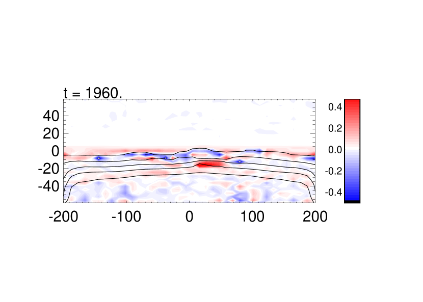
Figure 8: Spatial distribution of the index $\psi\equiv-d\rho/dz-\rho^{2}g_{0}/(\gamma p)$. at the location shown by the white box in Fig. 2. Color contour indicates $\psi$ (blue represents negative), while magnetic field lines are overplotted by solid lines. The aspect ratio is arranged. The index $\psi$ is negative around the area of the further evolution ($x/H_{0}=20,\,z/H_{0}=0$), indicating that this area is subject to the Parker instability.

that is, the area with negative $\psi$ is subject to the instability. Figure 8 illustrates the $\psi$ distribution with field lines just before the second-step emergence at $t/\tau_{0}=1960$. This figure indicates that the index $\psi$ is negative at around the point of emergence; we can conclude that the further evolution to the corona is ascribed by the Parker instability.

At $t/\tau_{0}=1960$, plasma $\beta\equiv p/(B^{2}/8\pi)$ is order of unity ($\sim 2$) and the magnetic field strength is about 700 G at the low photosphere within the emergent area, which are consistent with observations (e.g. Watanabe et al., 2008).

3.4 Fourth Stage ($t/\tau_{0}>2000$)

In this final phase, the magnetic flux emerging within the photosphere begins to expand to the solar corona by the magnetic pressure on the condition that the gas pressure acting on the surface of the flux is weak enough (Figs. 2-2). The expanding loop finally forms a large coronal loop. This process is similar to that of the results of classical calculations (e.g. Shibata et al., 1989, etc.).

The characteristics of this nonlinear phase is a self-similar evolution. Figures 9-9 indicate the distributions of the vertical component of velocity, gas density, and horizontal magnetic field strength along the axis $x/H_{0}=20$, where the apex of the loop is located (see Figs. 2 and 2), at $t/\tau_{0}=2000$, 2020, and 2040. According to Shibata et al. (1989), the expansion law is written as

$$V_{z}/C_{\rm s0} = a\,z/H_{0},$$ (17a)

$$\rho \propto z^{-4},$$ (17b)

$$B_{x} \propto z^{-1},$$ (17c)

where $a=0.05-0.07$ is about half the non-dimensional linear growth rate for plasma $\beta=0.5-2.0$ of the flux sheet. In our study, plasma $\beta$ of the magnetic field has been calculated to be 2 at $t/\tau_{0}=1960$ before the further evolution begins (see Section 3.3), which suggests that the velocity-height relation is

$$V_{z}/C_{\rm s0}\sim 0.05\,z/H_{0}.$$ (18)

This relation is overplotted in Figure 9 with a solid line. The other relations given by equations (17b) and (17c) are also overplotted in Figures 9 and 9 with solid lines. As seen from Figure 9, the nonlinear growth to the solar corona is consistent with that of Shibata et al. (1989).

The size of the coronal loop at $t/\tau_{0}=2070$ is found to be of $400H_{0}=80,000{\rm\,km}$ width and $200H_{0}=40,000{\rm\,km}$ height, while, at the surface, plasma $\beta$ is of the order of unity and the field strength is about $4B_{0}(=1200{\rm\,G})$.

4 Parameter Survey and Discussion

We carry out a parameter survey by changing the values of the initial field strength $B_{x}$ and the total magnetic flux $\Phi$ of the emerging flux sheet to investigate the condition of the sheet’s behavior. A summary of the values of $B_{x}$ and $\Phi$ under consideration is given in Table 1. Figure 10 shows the results of the parameter survey, where diamonds, asterisks, and X’s represent ‘two-step,’ ‘direct,’ and ‘failed’ evolution, respectively. Fluxes belong to the direct emergence group do evolve into the corona, however, they do not reveal the deceleration, unlike fluxes of the two-step emergence, while those of the failed emergence fragment within the convection zone or cannot pass through the photosphere. Figure 11 indicates height-time relations of the fluxes along the axis $x/H_{0}=0$. In this section, we will discuss each group in detail.

4.1 Direct emergence

In cases 2 and 3, the fluxes show the emergence to the corona without any deceleration at the surface. In other words, they ‘directly’ emerge to the corona. As shown in Figure 11, the height-time curves of cases 2 and 3 do not have an inflection point. We name them the ‘direct emergence’ group. The absence of an inflection implies that their evolutions are not affected by the isothermal photosphere/chromosphere at all since they have extremely strong field (note that these cases can be found in the upper right of Fig. 10).

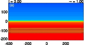
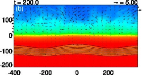
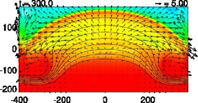
Figure 12: Time-evolution of the ‘direct emergence’ for case 2. 12 $t/\tau_{0}=0$; 12 $t/\tau_{0}=200$; 12 $t/\tau_{0}=300$. Logarithmic density profiles ($\log_{10}{(\rho/\rho_{0})}$) are indicated by color contour, while magnetic field lines and velocity vectors are overplotted with black lines and arrows.

Figure 12 shows the time evolution of the density profile, magnetic field lines, and velocity vectors for case 2. Color contour is the same as that of Fig. 2. Each flux of this group exhibits field strength $B\sim 10^{4}\ {\rm G}$ and plasma $\beta\sim 0.1$ at the surface after the emergence, which is not consistent with observations. Therefore, ‘direct emergence’ model is not suited for the formation model of active regions.

4.2 Two-step emergence

Cases 4-7 show the ‘two-step emergence’ to the corona as well as case 1 (typical model). Height-time relations of this group are shown in Fig. 11. Each line of this group has an inflection point beneath the surface ($z/H_{0}=0$), that is, rise velocity of the emerging flux turns from acceleration to deceleration phase within the convection zone due to the isothermal photosphere/chromosphere. As the figure indicates, the temporal length of the rising stage decreases with increasing initial field strength and total flux.

Among these five cases, cases 4, 5, and 6 show unrealistically strong flux densities $B\sim 10^{4}\ {\rm G}$ (plasma $\beta\sim 0.1$) at the photosphere after the coronal loops are built up. The realistic models of the formation of active regions are cases 1 and 7 ($\Phi=10^{21}-10^{22}\ {\rm Mx}$ with $B_{x}=10^{4}\ {\rm G}$ at $z=-20,000\ {\rm km}$). This result gives an important suggestion that the fluxes which form active regions are likely to have experienced the ‘two-step emergence.’

Our numerical results agree with recent satellite data. Otsuji et al. (2010) found the deceleration and the horizontal spreading of an emerging flux within the solar chromosphere by using Hinode/SOT. This observation supports the concept of the ‘two-step emergence’ model. At the same time, there is a difference between our results and the observation. The deceleration occurs in the chromosphere, not beneath the surface. The difference may partly come from the structure of the emerging loop. The numerical flux considered here has a sheet-like structure, on which the plasma piles continuously during its evolution (see Section 3). If the emerging loop is part of a (twisted) flux tube, the plasma on the loop can drain around the cross-section of the tube. Therefore, the emerging flux tube may rise through the convection zone faster than the sheet-like flux, and the tube may suffer a deceleration at a higher altitude when the tube itself passes through the convectively stable layers. On the other hand, Magara (2001) reported that even in case with an initial twisted tube, there is a deceleration close to the photosphere. The attribution of the deceleration altitude to the structure of the magnetic flux is still oversimplified at this moment. More quantitative study by three-dimensional simulations concerning with this issue is necessary.

It is possible that the emerging flux suffers a deceleration beneath the surface and exhibits the ‘two-step’ evolution, or, in some cases, fluxes show the ‘multi-step’ emergence since the structure of the rising loop in the convection zone cannot be achieved by the optical observations. To know the structure and the behavior of the flux emergence below the photosphere, advanced local helioseismology is needed (e.g. Sekii et al., 2007).

4.3 Failed emergence

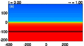
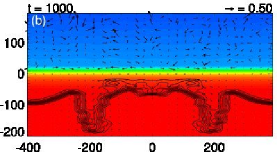
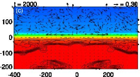
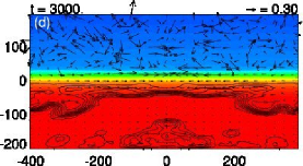
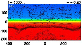
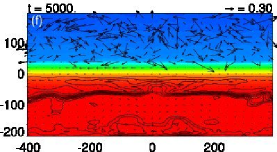
Figure 13: Time-evolution of the ‘failed emergence’ for case 14. 13 $t/\tau_{0}=0$; 13 $t/\tau_{0}=1000$; 13 $t/\tau_{0}=2000$; 13 $t/\tau_{0}=3000$; 13 $t/\tau_{0}=4000$; 13 $t/\tau_{0}=5000$. Logarithmic density profiles ($\log_{10}{(\rho/\rho_{0})}$) are indicated by color contour, while magnetic field lines and velocity vectors are overplotted with black lines and arrows.

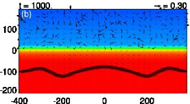
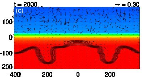
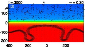
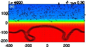
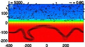
Figure 15: Time-evolution of the ‘failed emergence’ for case 8. 15 $t/\tau_{0}=0$; 15 $t/\tau_{0}=1000$; 15 $t/\tau_{0}=2000$; 15 $t/\tau_{0}=3000$; 15 $t/\tau_{0}=4000$; 15 $t/\tau_{0}=5000$. Logarithmic density profiles ($\log_{10}{(\rho/\rho_{0})}$) are indicated by color contour, while magnetic field lines and velocity vectors are overplotted with black lines and arrows.

Cases given in Fig. 10 with X’s belong to the ‘failed emergence’ group (cases 8-14). Fluxes of cases 9-14 suffer a fragmentation due to the continuous motion within the convection zone, so that further emergence does not occur (see Fig. 13). It is because the fluxes have weak fields compared to the local kinetic energy density of flow motion induced by the initial perturbation. Figure 14 shows the ratio of the magnetic energy density $E_{\rm mag}$ to the local kinetic energy density $E_{\rm kin}$ of case 14 along $x/H_{0}=0$ at $t/\tau_{0}=4000$ (Fig. 13), where $E_{\rm mag}=B^{2}/(8\pi)$ and $E_{\rm kin}=\rho v^{2}/2$, respectively. It reveals that the magnetic energy is weaker than the kinetic energy all over the convective layer. Height-time relations of these fluxes are presented in Figure 11. As the figure shows, each line of this group reveals a continuous fluctuation and remains around the surface, indicating that the continuous motion repeats within the solar interior. On the other hand, flux of case 8 do not show the secondary emergence because the flux fails to enhance the magnetic pressure gradient while crossing the surface. This flux keeps its coherency all the while since the field strength is almost in the same range as the local kinetic energy density (see Fig. 15).

Dotted line in Fig. 10 indicates the criteria for the ‘explosion’ of the emerging flux obtained by thin-flux-tube (TFT) approximation (Moreno-Insertis et al., 1995). They found that the rising tubes with a small amount of flux cannot reach the surface due to the ‘explosion’: if the tube rises sufficiently slowly, the stratification inside the tube gets close to a hydrostatic equilibrium along the field lines while the stratification outside is super-adiabatic. When the pressure difference between inside and outside the tube is small enough at the base of the convection zone, the difference decreases as the tube rises because the pressure gradient inside the tube is less steeper than that outside, so that the magnetic field at the apex can no longer be confined at a certain ‘explosion’ depth. According to their calculations, the tubes with the initial field strength and magnetic flux $(10^{4}\ {\rm G},\ 10^{22}\ {\rm Mx})$ and $(10^{5}\ {\rm G},\ 10^{17}\ {\rm Mx})$ at the base of the convection zone can reach close to the surface. Their field strength at $r/R_{\odot}=0.97$ ($z=-20,000\ {\rm km}$, i.e., the depth of our initial fluxes) are $3\times 10^{2}\ {\rm G}$ and $2\times 10^{4}\ {\rm G}$, respectively (see Moreno-Insertis et al., 1995, Fig. 1). We adopt them as criteria for the ‘non-explosion’. The majority of the fluxes with parameters in the range where they could not have reached at $z=-20,000\ {\rm km}$ according to the TFT model (left to the dotted line) also ceases emergence even in our MHD model.

There are, however, some cases in which, although the fluxes are expected to reach at $z=-20,000\ {\rm km}$ level by the TFT model, they fail to evolve further (cases 8, 9 and 10). Especially, case 8 ($10^{4}\ {\rm G}$ with $10^{20}\ {\rm Mx}$ at $z=-20,000\ {\rm km}$) reveals the photospheric field strength $B\sim 1\ {\rm G}$, indicating it could be the source of the magnetic fields in the quiet sun if the fields are enhanced, e.g., by the flux expulsion due to the magneto-convection at the surface. Interestingly, this flux maintains its coherency all the while and remains floating around beneath the surface after it fails the further evolution to the corona because it has a strong field that is in equipartition with the kinetic energy density (Fig. 15). This suggests that the flux of case 8 can be the origin of the ephemeral regions. Flux 8 has $10^{20}\ {\rm Mx}$, consistent with the flux of mid-sized ephemeral regions (Hagenaar, 2001).

5 Conclusions

We perform the nonlinear two-dimensional simulations to investigate the behavior of emerging flux from moderately deep convection zone ($z=-20,000\ {\rm km}$). We set a much wider numerical box ($160\ {\rm Mm}\times 80\ {\rm Mm}$) than those of the previous experiments on the Parker instability (e.g. Shibata et al., 1989).

In the typical case ($B=10^{4}\ {\rm G}$ with $\Phi=10^{21}\ {\rm Mx}$ at $z=-20,000\ {\rm km}$), the results show the ‘two-step emergence’. In the middle of the way of the first emergence to the solar surface, the flux loop turns from an acceleration phase to deceleration when approaching the (sub-adiabatically stratified, i.e., convectively stable) photosphere/chromosphere. The emerging flux has a sheet-like shape, thus it is difficult for the mass on the loop to escape from the area between the loop and the convectively stable surface. This mass pile-up causes the loop decelerate. The deceleration of the apex of the expanding flux and the continuous rising of the hillsides make loop flattened, which results in the plasma kept on the flux. This deceleration mechanism is another new one and different from those of the preceding studies (Magara, 2001; Archontis et al., 2004; Murray et al., 2006) with magnetic flux tubes in much smaller regions. However, our result predicts the behavior of a flux within the convection zone, provided the flux has a sheet-like structure . As a result of the deceleration and the flattening, the flux spreads sideways just beneath the surface, at which point the rise velocity of the crest of the loop is almost zero. Meanwhile, the flux is continuously transported from below, then the magnetic pressure gradient enhances locally in the photosphere. We found that the further evolution to the corona occurs on the basis of the Parker instability. At the point of the instability, plasma $\beta$ is calculated to be order of unity ($\sim 2$) and the magnetic field strength is about $700\ {\rm G}$. In the final stage, the flux shows the nonlinear evolution to the corona, which resembles the classical experiments (e.g. Shibata et al., 1989, etc.). The second-step evolution is described clearly by the expansion law by Shibata et al. (1989). We find that the coronal loop exhibits $80,000\ {\rm km}$ width with $40,000\ {\rm km}$ height, while the field strength of each footpoint at the surface is about $1200\ {\rm G}$.

We perform parameter runs by changing the initial field strength $B_{x}$ and the total flux $\Phi$ to investigate the condition of the ‘two-step emergence’. The results of the runs under considerations can be divided into three groups: ‘direct’, ‘two-step’, and ‘failed’ emergence. In case of the ‘direct emergence’, the flux do evolve to the corona, but they do not show the deceleration by the isothermal surface due to their strong initial magnetic fields ($10^{23}-10^{24}\ {\rm Mx}$ with $10^{5}\ {\rm G}$ at $z=-20,000\ {\rm km}$). The coronal loops present irregularly strong flux densities at the footpoints; thus, we conclude that they are not suitable for the formation models of active regions. As for the cases showing the ‘two-step emergence’, two out of five exhibit the favorable values of the photospheric field strength and plasma $\beta$. The others have so large values that they cannot be regarded as realistic models of active regions. We can say that active regions on the sun are likely to have undergone the deceleration and likely to show the ‘two-step emergence’ mentioned above. The condition for this ‘two-step’ active region is ranging from $10^{21}$ to $10^{22}\ {\rm Mx}$ with $10^{4}\ {\rm G}$ at $z=-20,000\ {\rm km}$ in the convection zone. Some recent observations support this two-step model. The cases with $B\lesssim 10^{4}\ {\rm G}$ reveal ‘failed’ evolutions; they fragment within the convection zone or cannot have sufficient magnetic pressure gradient to trigger the instability that the second-step emergence do not occur although the flux maintains its coherency. We have some discussions in connection with the results of the thin-flux-tube (TFT) model by Moreno-Insertis et al. (1995). The cases which are found to have ‘exploded’ in the deeper point in the TFT scheme also do not show further evolutions in our MHD scheme. However, there are some cases which escape the ‘explosion’ fail the second-step evolutions, one of which is possibly the source of the magnetic field in the quiet sun.

The present calculations are in a two-dimensional scheme solving simplified equations. Thus we have to demonstrate the more realistic experiments in 3D. At the same time, advanced observations by helioseismological technique are needed to reveal the detail of the emerging flux in the convection zone.

Figure 3: Time evolution of the apex of the flux sheet; solid line is a height of the apex, whose rise velocity is indicated with dashed line. Photospheric level ($z/H_{0}=0$) is overplotted with dotted line.

Figure 4: The close-up view of Fig. 3. Upward velocity at the apex of the loop is plotted by a dashed line, while the local Alfv$\acute{\rm e}$n speed is represented by a solid line.

Figure 5: Density differences from the initial state ($\Delta\rho\equiv\rho(t)-\rho(0)$, solid lines) and horizontal field components ($B_{x}$, dotted lines) along the $z$-axis at the center of the simulation box ($x/H_{0}=0$) at the three different times. As the magnetic flux rises, mass piles up on the loop. However, the mass cannot persist through the isothermal photosphere ($0<z/H_{0}<10$).

Figure 6: 6: Time evolution of the vertical components of the forces acting on the apex of the emerging loop: gas pressure gradient ($-\nabla p=-dp/dz$, solid line), gravity ($\rho g_{0}$, dotted line), magnetic pressure gradient ($-\nabla p_{\rm mag}=-d[B^{2}/(8\pi)]/dz$, dashed line), and magnetic tension ($t_{\rm mag}=[(\mbox{\boldmath$B$}\cdot\nabla)\mbox{\boldmath$B$}]_{z}/(4\pi)$, dashed-dotted line). 6: The same of the acceleration ($F_{z}/\rho=(-\nabla p-\rho g_{0}-\nabla p_{\rm mag}-t_{\rm mag})/\rho$). A dotted line shows that the acceleration equals zero.

Figure 7: Vertical distributions of magnetic pressure (solid line), gas pressure (dotted line), and gas density (dashed line) along the axis $x/H_{0}=20$ at $t/\tau_{0}=1960$, which is the central position of the second-step emergence.

Figure 9: 9: Distribution of the upward velocity along the vertical axis $x/H_{0}=20$. Dotted, dashed, and dash-dotted lines indicate the distribution at $t/\tau_{0}=2000$, $t/\tau_{0}=2020$, and $t/\tau_{0}=2040$, respectively. A solid line shows the theoretical velocity-height relation according to Shibata et al. (1989). 9: Distribution of the gas density along the axis $x/H_{0}=20$. The notation of lines is the same as in 9. 9: Distribution of the horizontal component of the magnetic field along the axis $x/H_{0}=20$. The notation of lines is the same as in 9.

Figure 10: Results of the parameter survey. Diamonds, asterisks, and X’s represent two-step emergence, direct emergence, and failed emergence, respectively. Case numbers are plotted on the lower right of each symbol. Criteria for the ‘explosion’ of the emerging flux obtained by thin-flux-tube approximation simulations (Moreno-Insertis et al., 1995) is overplotted with a dotted line.

Figure 11: 11: Time evolution of the height of the flux sheet along the axis $x/H_{0}=0$ for ‘direct emergence’ (cases 2 and 3). Dashed and dashed-dotted lines represent evolutions of cases 2 and 3, respectively, while solid line is the height-time relation of case 1 (typical model). 11: Same for ‘two-step emergence’ (cases 1 and 4-7). Solid, dashed, dashed-dotted, dashed-dotted-dotted-dotted, and long-dashed lines represent evolutions of cases 1, 4, 5, 6, and 7, respectively. 11: Same for ‘failed emergence’ (cases 8-14). Dashed (thick), dash-dotted (thick), long-dashed (thick), dashed-dotted-dotted-dotted, dashed (thin), and dash-dotted (thin), long-dashed (thin) lines represent evolutions of cases 8, 9, 10, 11, 12, 13, and 14, respectively, while solid line is the height-time relation of case 1 (typical model). In each panel, dotted line is overpoltted to show the surface level ($z/H_{0}=0$).

Figure 14: The ratio of $E_{\rm mag}=B^{2}/(8\pi)$ to $E_{\rm kin}=\rho v^{2}/2$ of case 14 along $x/H_{0}=0$ at $t/\tau_{0}=4000$.

Table 1: Summary of Cases

case	$B_{x}$ [G]	$\Phi$ [Mx]	$\beta_{*}$	$D$ [km]	$N_{x}\times N_{z}$
1	$1.0\times 10^{4}$	$1.0\times 10^{21}$	$1.6\times 10^{2}$	1000	$1536\times 1920$
2	$8.1\times 10^{4}$	$9.8\times 10^{23}$	$1.1\times 10^{-1}$	11,000	$1024\times 1280$
3	$1.0\times 10^{5}$	$1.0\times 10^{23}$	$2.0\times 10^{-1}$	3000	$1024\times 1280$
4	$1.1\times 10^{5}$	$1.0\times 10^{22}$	$2.0\times 10^{-1}$	840	$1024\times 1280$
5	$1.1\times 10^{5}$	$1.1\times 10^{21}$	$2.0\times 10^{-1}$	200	$1024\times 1280$
6	$1.1\times 10^{4}$	$1.1\times 10^{23}$	$2.2\times 10^{2}$	11,400	$1024\times 1280$
7	$1.0\times 10^{4}$	$1.0\times 10^{22}$	$1.6\times 10^{2}$	3200	$1024\times 1280$
8	$8.9\times 10^{3}$	$1.0\times 10^{20}$	$1.5\times 10^{2}$	260	$1024\times 1280$
9	$1.1\times 10^{3}$	$1.0\times 10^{22}$	$2.2\times 10^{4}$	11,000	$1024\times 1280$
10	$1.0\times 10^{3}$	$1.0\times 10^{21}$	$1.6\times 10^{4}$	3200	$1024\times 1280$
11	$9.9\times 10^{2}$	$1.1\times 10^{20}$	$1.5\times 10^{4}$	1000	$1024\times 1280$
12	$1.0\times 10^{2}$	$1.0\times 10^{21}$	$2.5\times 10^{6}$	11,400	$1024\times 1280$
13	$1.1\times 10^{2}$	$1.0\times 10^{20}$	$1.4\times 10^{6}$	3200	$1024\times 1280$
14	$1.0\times 10^{2}$	$1.0\times 10^{19}$	$1.4\times 10^{6}$	960	$1024\times 1280$

References

- Abbett & Fisher (2003) Abbett, W. P., & Fisher, G. H. 2003, ApJ, 582, 475
- Acheson (1979) Acheson, D. J. 1979, Sol. Phys., 62, 23
- Archontis et al. (2004) Archontis, V., Moreno-Insertis, F., Galsgaard, K., Hood, A., & O’Shea, E. 2004, A&A, 426, 1047
- Caligari et al. (1995) Caligari, P., Moreno-Insertis, F., & Schssler, M. 1995, ApJ, 441, 886
- Cheung et al. (2008) Cheung, M. C. M., Schssler, M., Tarbel, T. D., & Title, A. M. 2008, ApJ, 687, 1373
- D’Silva & Choudhuri (1993) D’Silva, S., & Choudhuri, A. R. 1993, A&A, 272, 621
- Fan (2001a) Fan, Y. 2001a, ApJ, 546, 509
- Fan (2001b) Fan, Y. 2001b, ApJ, 554, L111
- Fan (2004) Fan, Y. 2004, Living Rev. Solar Phys., 1, 1
- Gough (1969) Gough, D. O. 1969, J. Atmos. Sci., 26, 448
- Hagenaar (2001) Hagenaar, H. J. 2001, ApJ, 555, 448
- Lantz & Fan (1999) Lantz, S. R., & Fan, Y. 1999, ApJS, 121, 247
- Magara (2001) Magara, T. 2001, ApJ, 549, 608
- Matsumoto et al. (1993) Matsumoto, R., Tajima, T., Shibata, K., & Kaisig, M. 1993, ApJ, 414, 357
- Moreno-Insertis et al. (1995) Moreno-Insertis, F., Caligari, P., & Schssler, M. 1995, ApJ, 452, 894
- Murray et al. (2006) Murray, M. J., Hood, A. W., Moreno-Insertis, F., Galsgaard, K., & Archontis, V. 2006, A&A, 460, 909
- Newcomb (1961) Newcomb, W. A. 1961, Phys. Fl., 4, 391
- Nozawa et al. (1992) Nozawa, S., Shibata, K., Matsumoto, R., Sterling, A. C., Tajima, T., Uchida, Y., Ferrari, A., & Rosner, R. 1992, ApJS, 78, 267
- Otsuji et al. (2010) Otsuji, K. et al. 2010, PASJ, in press
- Parker (1955) Parker, E. N. 1955, ApJ, 121, 491
- Parker (1966) Parker, E. N. 1966, ApJ, 145, 811
- Parker (1975) Parker, E. N. 1975, ApJ, 198, 205
- Sekii et al. (2007) Sekii, T., et al. 2007, PASJ, 59, S637
- Shibata et al. (1989) Shibata, K., Tajima, T., Steinolfson, R. S., & Matsumoto, R. 1989, ApJ, 345, 584
- Spruit (1981) Spruit, H. C. 1981, A&A, 98, 155
- Tsuneta et al. (2008) Tsuneta, S. et al. 2008, Sol. Phys., 249, 167
- Watanabe et al. (2008) Watanabe, H., Kitai, R., Okamoto, K., Nishida, K., Kiyohara, J., Ueno, S., Hagino, M., Ishii, T. T., & Shibata, K. 2008 ApJ, 684, 736
- Yokoyama & Shibata (1995) Yokoyama, T., & Shibata, K. 1995, Nature, 375, 42
- Yokoyama & Shibata (1996) Yokoyama, T., & Shibata, K. 1996, PASJ, 48, 353