Abstract

Results on the behaviour of the rightmost particle in the $n$th generation in the branching random walk are reviewed and the phenomenon of anomalous spreading speeds, noticed recently in related deterministic models, is considered. The relationship between such results and certain coupled reaction-diffusion equations is indicated.

Chapter 0 Branching out

John D. Biggins

AMS subject classification (MSC2010)

60J80

1 Introduction

I arrived at the University of Oxford in the autumn of 1973 for postgraduate study. My intention at that point was to work in Statistics. The first year of study was a mixture of taught courses and designated reading on three areas (Statistics, Probability, and Functional Analysis, in my case) in the ratio 2:1:1 and a dissertation on the main area. As part of the Probability component, I attended a graduate course that was an exposition, by its author, of the material in Hammersley, (1974), which had grown out of his contribution to the discussion of John’s invited paper on subadditive ergodic theory (Kingman,, 1973). A key point of Hammersley’s contribution was that the postulates used did not cover the time to the first birth in the $n$th generation in a Bellman–Harris process. Hammersley, (1974) showed, among other things, that these quantities did indeed exhibit the anticipated limit behaviour in probability. I decided not to be examined on this course, which was I believe a wise decision, but I was intrigued by the material. That interest turned out to be critical a few months later.

By the end of the academic year I had concluded that I wanted to pursue research in Probability rather than Statistics and asked to have John as supervisor. He agreed. Some time later we met and he asked me whether I had any particular interests already—I mentioned Hammersley’s lectures. When I met him he was in the middle of preparing something (which I could see, but not read upside down). He had what seemed to be a pile of written pages, a part written page and a pile of blank paper. There was nothing else on the desk. A few days later a photocopy of a handwritten version of Kingman, (1975), essentially identical to the published version, appeared in my pigeon-hole with the annotation “the multitype version is an obvious problem”—I am sure this document was what he was writing when I saw him. (Like all reminiscences, this what I recall, but it is not necessarily what happened.) This set me going. For the next two years, it was a privilege to have John as my thesis supervisor. He supplied exactly what I needed at the time: an initial sense of direction, a strong encouragement to independence, an occasional nudge on the tiller about what did or did not seem tractable, the discipline of explaining orally what I had done, and a ready source on what was known, and where to look for it. However, though important, none of these get to the heart of the matter, which is that I am particularly grateful to have had that period of contact with, and opportunity to appreciate first-hand, such a gifted mathematician.

Kingman, (1975) considered the problem Hammersley had raised in its own right, rather than as an example of, and adjunct to, the general theory of subadditive processes. Here, I will say something about some recent significant developments on the first-birth problem. I will also go back to my beginnings, by outlining something new about the multitype version that concerns the phenomenon of ‘anomalous spreading speeds’, which was noted in a related context in Weinberger et al., (2007). Certain martingales were deployed in Kingman, (1975). These have been a fruitful topic in their own right, and have probably received more attention since then than the first-birth problem itself (see Alsmeyer and Iksanov, (2009) for a recent nice contribution on when these martingales are integrable). However, those developments will be ignored here.

2 The basic model

The branching random walk (BRW) starts with a single particle located at the origin. This particle produces daughter particles, which are scattered in $\mathbb{R}$, to give the first generation. These first generation particles produce their own daughter particles similarly to give the second generation, and so on. Formally, each family is described by the collection of points in $\mathbb{R}$ giving the positions of the daughters relative to the parent. Multiple points are allowed, so that in a family there may be several daughter particles born in the same place. As usual in branching processes, the $n$th generation particles reproduce independently of each other. The process is assumed supercritical, so that the expected family size exceeds one (but need not be finite—indeed even the family size itself need not be finite). Let $\mathbf{P}$ and $\mathbf{E}$ be the probability and expectation for this process and let $Z$ be the generic reproduction process of points in $\mathbb{R}$. Thus, $\mathbf{E}Z$ is the intensity measure of $Z$ and $Z(\mathbb{R})$ is the family size, which will also be written as $N$. The assumption that the process is supercritical becomes that $\mathbf{E}Z(\mathbb{R})=\mathbf{E}N>1$. To avoid burdening the description with qualifications about the survival set, let $\mathbf{P}(N=0)=0$, so that the process survives almost surely.

The model includes several others. One is when each daughter receives an independent displacement, another is when all daughters receive the same displacement, with the distribution of the displacement being independent of family size in both cases. These will be called the BRW with independent and common displacements respectively. Obviously, in both of these any line of descent follows a trajectory of a random walk. (It is possible to consider an intermediate case, where displacements have these properties conditional on family size, but that is not often done.) Since family size and displacements are independent, these two processes can be coupled in a way that shows that results for one will readily yield results for the other. In a common displacement BRW imagine each particle occupying the (common) position of its family. Then the process becomes an independent displacement BRW, with a random origin given by the displacement of the first family, and its $n$th generation occupies the same positions as the $(n+1)$th generation in the original common displacement BRW. Really this just treats each family as a single particle.

In a different direction, the points of $Z$ can be confined to $(0,\infty)$ and interpreted as the mother’s age at the birth of that daughter: the framework adopted in Kingman, (1975). Then the process is the general branching process associated with the names of Ryan, Crump, Mode and Jagers. Finally, when all daughters receive the same positive displacement with a distribution independent of family size the process is the Bellman–Harris branching process: the framework adopted in Hammersley, (1974).

There are other ‘traditions’, which consider the BRW but introduce and describe it rather differently and usually with other problems in focus. There is a long tradition phrased in terms of ‘multiplicative cascades’ (see for example Liu, (2000) and the references there) and a rather shorter one phrased in terms of ‘weighted branching’ (see for example Alsmeyer and Rösler, (2006) and the references there). The model has arisen in one form or another in a variety of areas. The most obvious is as a model for a population spreading through an homogeneous habitat. It has also arisen in modelling random fractals (Peyrière,, 2000) commonly in the language of multiplicative cascades, in the theoretical study of algorithms (Mahmoud,, 1992), in a problem in group theory (Abért and Virág,, 2005) and as an ersatz for both lattice-based models of spin glasses in physics (Koukiou,, 1997) and a number theory problem (Lagarias and Weiss,, 1992).

3 Spreading out: old results

Let $Z^{(n)}$ be the positions occupied by the $n$th generation and ${B}^{(n)}$ its rightmost point, so that

$${B}^{(n)}=\sup\{z:z\mbox{\leavevmode\nobreak\ a point of\leavevmode\nobreak\ }Z^{(n)}\}.$$

One can equally well consider the leftmost particle, and the earliest studies did that. Reflection of the whole process around the origin shows the two are equivalent: all discussion here will be expressed in terms of the rightmost particle. The first result, stated in a moment, concerns ${B}^{(n)}/n$ converging to a constant, $\Gamma$, which can reasonably be interpreted as the speed of spread in the positive direction.

A critical role in the theory is played by the Laplace transform of the intensity measure $\mathbf{E}Z$: let $\kappa(\phi)=\log\int e^{\phi z}\mathbf{E}Z(dz)$ for $\phi\geq 0$ and $\kappa(\phi)=\infty$ for $\phi<0$. It is easy to see that when this is finite for some $\phi>0$ the intensity measures of $Z$ and $Z^{(n)}$ are finite on bounded sets, and decay exponentially in their right tail. The behaviour of the leftmost particle is governed by the behaviour of the transform for negative values of its argument. The definition of $\kappa$ discards these, which simplifies later formulations by automatically keeping attention on the right tail. In order to give one of the key formulae for $\Gamma$ and for later explanation, let ${\kappa}^{\ast}$ be the Fenchel dual of $\kappa$, which is the convex function given by

$${\kappa}^{\ast}(a)=\sup_{\theta}\{\theta a-\kappa(\theta)\}.$$ (3.1)

This is sufficient notation to give the first result.

Theorem 3.1.

When there is a $\phi>0$ such that

$$\kappa(\phi)<\infty,$$ (3.2)

there is a constant $\Gamma$ such that

$$\frac{{B}^{(n)}}{n}\rightarrow\Gamma\mbox{\leavevmode\nobreak\ \leavevmode\nobreak\ \leavevmode\nobreak\ a.s}.$$ (3.3)

and $\Gamma=\sup\{a:{\kappa}^{\ast}(a)<0\}=\inf\{\kappa(\theta)/\theta:\theta\}$.

This result was proved for the common BRW with only negative displacements with convergence in probability in Hammersley, (1974, Theorem 2). It was proved in Kingman, (1975, Theorem 5) for $Z$ concentrated on $(-\infty,0)$ and with $0<\kappa(\phi)<\infty$ instead of (3.2). The result stated above is contained in Biggins, (1976a, Theorem 4), which covers the irreducible multitype case also, of which more later. The second of the formulae for $\Gamma$ is certainly well-known but cannot be found in the papers mentioned—I am not sure where it first occurs. It is not hard to establish from the first one using the definition and properties of ${\kappa}^{\ast}$.

The developments described here draw on features of transform theory, to give properties of $\kappa$, and of convexity theory, to give properties of ${\kappa}^{\ast}$ and the speed $\Gamma$. There are many presentations of, and notations for, these, tailored to the particular problem under consideration. In this review, results will simply be asserted. The first of these provides a context for the next theorem and aids interpretation of $\sup\{a:{\kappa}^{\ast}(a)<0\}$ in the previous one. It is that when $\kappa$ is finite somewhere on $(0,\infty)$, ${\kappa}^{\ast}$ is an increasing, convex function, which is continuous from the left, with minimum value $-\kappa(0)=-\log\mathbf{E}N$, which is less than zero.

A slight change in focus derives Theorem 3.1 from the asymptotics of the numbers of particles in suitable half-infinite intervals. As part of the derivation of this the asymptotics of the expected numbers are obtained. Specifically, it is shown that when (3.2) holds

$$n^{-1}\log\left(\mathbf{E}Z^{(n)}[na,\infty)\right)\rightarrow-{\kappa}^{\ast}(a)$$

(except, possibly, at one $a$). The trivial observation that when the expectation of integer-valued variables decays geometrically the variables themselves must ultimately be zero implies that $\log Z^{(n)}[na,\infty)$ is ultimately infinite on $\{a:{\kappa}^{\ast}(a)>0\}$. This motivates introducing a notation for sweeping positive values of ${\kappa}^{\ast}$, and later other functions, to infinity and so we let

$${f}^{{\circ}}(a)=\left\{\begin{array}[]{ll}f(a)&\mbox{when\leavevmode\nobreak\ }f(a)\leq 0\\ \infty&\mbox{when\leavevmode\nobreak\ }f(a)>0\end{array}\right.$$ (3.4)

and ${\kappa}^{\ast\!\!\!\circ}={({\kappa}^{\ast})}^{{\circ}}$. The next result can be construed as saying that in crude asymptotic terms this is the only way actual numbers differ from their expectation.

Theorem 3.2.

When (3.2) holds,

$$\frac{1}{n}\log\left(Z^{(n)}[na,\infty)\right)\rightarrow-{\kappa}^{\ast\!\!\!\circ}(a)\mbox{\leavevmode\nobreak\ \leavevmode\nobreak\ \leavevmode\nobreak\ a.s.},$$ (3.5)

for all $a\neq\Gamma$.

From this result, which is Biggins, (1977a, Theorem 2), and the properties of ${\kappa}^{\ast\!\!\!\circ}$, Theorem 3.1 follows directly.

A closely related continuous-time model arises when the temporal development is a Markov branching process (Bellman–Harris with exponential lifetimes) or even a Yule process (binary splitting too) and movement is Brownian, giving binary branching Brownian motion. The process starts with a single particle at the origin, which then moves with a Brownian motion with variance parameter $V$. This particle splits in two at rate $\lambda$, and the two particles continue, independently, in the same way from the splitting point. (Any discrete skeleton of this process is a branching random walk.)

Now, let ${B}^{(t)}$ be the position of the rightmost particle at time $t$. Then $u(x,t)=\mathbf{P}({B}^{(t)}\leq x)$ satisfies the (Fisher/Kolmogorov–Petrovski–Piscounov) equation

$$\frac{\partial u}{\partial t}=V\frac{1}{2}\frac{\partial^{2}u}{\partial x^{2}}-\lambda u(1-u),$$ (3.6)

which is easy to see informally by conditioning on what happens in $[0,\delta t]$. The deep studies of Bramson, (1978a, 1983) show, among other things, that (with $V=\lambda=1$) ${B}^{(t)}$ converges in distribution when centred on its median and that median is (to $O(1)$)

$$\sqrt{2}t-\frac{1}{\sqrt{2}}\left(\frac{3}{2}\log t\right),$$

which implies that $\Gamma=\sqrt{2}$ here. For the skeleton at integer times, $\kappa(\theta)=\theta^{2}/2+1$ for $\theta\geq 0$, and using Theorem 3.1 on this confirms that $\Gamma=\sqrt{2}$. Furthermore, for later reference, note that $\theta\Gamma-\kappa(\theta)=0$ when $\theta=\sqrt{2}$.

Theorem 3.1 is for discrete time, counted by generation. There are corresponding results for continuous time, where the reproduction is now governed by a random collection of points in time and space ($\mathbb{R}^{+}\!\times\mathbb{R}$). The first component gives the mother’s age at the birth of this daughter and the second that daughter’s position relative to her mother. Then the development in time of the process is that of a general branching process rather than the Galton–Watson development that underpins Theorem 3.1. This extension is discussed in Biggins, (1995) and Biggins, (1997). In it particles may also move during their lifetime and then branching Brownian motion becomes a (very) special case. Furthermore, there are also natural versions of Theorems 3.1 and 3.2 when particle positions are in $\mathbb{R}^{d}$ rather than $\mathbb{R}$—see Biggins, (1995, §4.2) and references there.

4 Spreading out: first refinements

Obviously rate-of-convergence questions follow on from (3.3). An aside in Biggins, (1977b, p33) noted that, typically, ${B}^{(n)}-n\Gamma$ goes to $-\infty$. The following result on this is from Biggins, (1998, Theorem 3), and much of it is contained also in Liu, (1998, Lemma 7.2). When $\mathbf{P}(Z(\Gamma,\infty)>0)>0$, so displacements greater than $\Gamma$ are possible, and (3.2) holds, there is a finite $\vartheta>0$ with $\vartheta\Gamma-\kappa(\vartheta)=0$. Thus the condition here, which will recur in later theorems, is not restrictive.

Theorem 4.1.

If there is a finite $\vartheta>0$ with $\vartheta\Gamma-\kappa(\vartheta)=0$, then

$${B}^{(n)}-n\Gamma\rightarrow-\infty\mbox{\leavevmode\nobreak\ \leavevmode\nobreak\ \leavevmode\nobreak\ a.s.,}$$ (4.1)

and the condition is also necessary when $\mathbf{P}(Z(\Gamma,\infty)>0)>0$.

The theorem leaves some loose ends when $\mathbf{P}(Z(\Gamma,\infty)=0)=1$. Then ${B}^{(n)}-n\Gamma$ is a decreasing sequence, and so it does have a limit, but whether (4.1) holds or not is really the explosion (i.e. regularity) problem for the general branching process: whether, with a point $z$ from $Z$ corresponding to a birth time of $\Gamma-z$, there can be an infinite number of births in a finite time. This is known to be complex—see Grey, (1974) for example. In the simpler cases it is properties of $Z(\{\Gamma\})$, the number of daughters displaced by exactly $\Gamma$, that matters.

If $Z(\{\Gamma\})$ is the family size of a surviving branching process (so either $\mathbf{E}Z(\{\Gamma\})>1$ or $\mathbf{P}(Z(\{\Gamma\})=1)=1$) it is easy to show that $({B}^{(n)}-n\Gamma)$ has a finite limit—so (4.1) fails—using embedded surviving processes resulting from focusing on daughters displaced by $\Gamma$: see Biggins, (1976b, Proposition II.5.2) or Dekking and Host, (1991, Theorem 1). In a similar vein, with extra conditions, Addario-Berry and Reed, (2009, Theorem 4) show $\mathbf{E}({B}^{(n)}-n\Gamma)$ is bounded.

Suppose now that (3.2) holds. When $\mathbf{P}(Z(a,\infty)=0)=1$, simple properties of transforms imply that $\theta a-\kappa(\theta)\uparrow-\log\mathbf{E}Z(\{a\})$ as $\theta\uparrow\infty$. Then, when $\mathbf{E}Z(\{a\})<1$ a little convexity theory shows that $\Gamma<a$ and that there is a finite $\vartheta$ with $\vartheta\Gamma-\kappa(\vartheta)=0$, so that Theorem 4.1 applies. This leaves the case where (3.2) holds, $\mathbf{P}(Z(\Gamma,\infty)=0)=1$ and $\mathbf{E}Z(\{\Gamma\})=1$ but $\mathbf{P}(Z(\{\Gamma\})=1)<1$, which is sometimes called, misleadingly in my opinion, the critical branching random walk because the process of daughters displaced by exactly $\Gamma$ from their parent forms a critical Galton–Watson process. For this case, Bramson, (1978b, Theorem 1) and Dekking and Host, (1991, §9) show that (4.1) holds under extra conditions including that displacements lie in a lattice, and that the convergence is at rate $\log\log n$. Bramson, (1978b, Theorem 2) also gives conditions under which (4.1) fails.

5 Spreading out: recent refinements

The challenge to derive analogues for the branching random walk of the fine results for branching Brownian motion has been open for a long time. Progress was made in McDiarmid, (1995) and, very recently, a nice result has been given in Hu and Shi, (2009, Theorem 1.2), under reasonably mild conditions. Here is its translation into the current notation. It shows that the numerical identifications noted in the branching Brownian motion case in §3 are general.

Theorem 5.1.

Suppose that there is a $\vartheta>0$ with $\vartheta\Gamma-\kappa(\vartheta)=0$, and that, for some $\epsilon>0$, $\mathbf{E}(N^{1+\epsilon})<\infty$, $\kappa(\vartheta+\epsilon)<\infty$ and $\int e^{-\epsilon z}\mathbf{E}Z(dz)<\infty$. Then

$$-\frac{3}{2}=\liminf_{n}\frac{\vartheta({B}^{(n)}-n\Gamma)}{\log n}<\limsup_{n}\frac{\vartheta({B}^{(n)}-n\Gamma)}{\log n}=-\frac{1}{2}\mbox{\leavevmode\nobreak\ \leavevmode\nobreak\ \leavevmode\nobreak\ a.s.}$$

and

$$\frac{\vartheta({B}^{(n)}-n\Gamma)}{\log n}\rightarrow-\frac{3}{2}\mbox{\leavevmode\nobreak\ \leavevmode\nobreak\ in probability}.$$

Good progress has also been made on the tightness of the distributions of ${B}^{(n)}$ when centred suitably. Here is a recent result from Bramson and Zeitouni, (2009, Theorem 1.1).

Theorem 5.2.

Suppose the BRW has independent or common displacements according to the random variable $X$. Suppose also that for some $\epsilon>0$, $\mathbf{E}(N^{1+\epsilon})<\infty$ and that for some $\psi>0$ and $y_{0}>0$

$$\mathbf{P}(X>x+y)\leq e^{-\psi y}\mathbf{P}(X>x)\leavevmode\nobreak\ \leavevmode\nobreak\ \leavevmode\nobreak\ \leavevmode\nobreak\ \forall x>0,y>y_{0}.$$ (5.1)

Then the distributions of $\{{B}^{(n)}\}$ are tight when centred on their medians.

It is worth noting that (5.1) ensures that (3.2) holds for all $\phi\in[0,\psi)$. There are other results too—in particular, McDiarmid, (1995, Theorem 1) and Dekking and Host, (1991, §3) both give tightness results for the (general) BRW, but with $Z$ concentrated on a half-line. Though rather old for this section, Dekking and Host, (1991, Theorem 2) is worth recording here: the authors assume the BRW is concentrated on a lattice, but they do not use that in the proof of this theorem. To state it, let $\widetilde{D}$ be the second largest point in $Z$ when $N\geq 2$ and the only point otherwise.

Theorem 5.3.

If the points of $Z$ are confined to $(-\infty,0]$ and $\mathbf{E}\widetilde{D}$ is finite, then $\mathbf{E}{B}^{(n)}$ is finite and the distributions of $\{{B}^{(n)}\}$ are tight when centred on their expectations.

The condition that $\mathbf{E}\widetilde{D}$ is finite holds when $\int e^{\phi z}\mathbf{E}Z(dz)$ is finite in a neighbourhood of the origin, which is contained within the conditions in Theorem 5.1. In another recent study Addario-Berry and Reed, (2009, Theorem 3) give the following result, which gives tightness and also estimates the centring.

Theorem 5.4.

Suppose that there is a $\vartheta>0$ with $\vartheta\Gamma-\kappa(\vartheta)=0$, and that, for some $\epsilon>0$, $\kappa(\vartheta+\epsilon)<\infty$ and $\int e^{-\epsilon z}\mathbf{E}Z(dz)<\infty$. Suppose also that the BRW has a finite maximum family size and independent displacements. Then

$$\mathbf{E}{B}^{(n)}=n\Gamma-\frac{3}{2\vartheta}\log n+O(1),$$

and there are $C>0$ and $\delta>0$ such that

$$\mathbf{P}\left(|{B}^{(n)}-\mathbf{E}{B}^{(n)}|>x\right)\leq Ce^{-\delta x}\leavevmode\nobreak\ \leavevmode\nobreak\ \leavevmode\nobreak\ \forall x.$$

The conditions in the first sentence here have been stated in a way that keeps them close to those in Theorem 5.1 rather than specialising them for independent displacements. Now, moving from tightness to convergence in distribution—which cannot be expected to hold without a non-lattice assumption—the following result, which has quite restrictive conditions, is taken from Bachmann, (2000, Theorem 1).

Theorem 5.5.

Suppose that the BRW has $\mathbf{E}N<\infty$ and independent displacements according to a random variable with density function $f$ where $-\log f$ is convex. Then the variables ${B}^{(n)}$ converge in distribution when centred on medians.

It is not hard to use the coupling mentioned in §2 to see that Theorems 5.4 and 5.5 imply that these two results also hold for common displacements.

6 Deterministic theory

There is another, deterministic, stream of work concerned with modelling the spatial spread of populations in a homogeneous habitat, and closely linked to the study of reaction-diffusion equations like (3.6). The main presentation is Weinberger, (1982), with a formulation that has much in common with that adopted in Hammersley, (1974). Here the description of the framework is pared-down. This sketch draws heavily on Weinberger, (2002), specialised to the homogeneous (i.e. aperiodic) case and one spatial dimension. The aim is to say enough to make certain connections with the BRW.

Let $u^{(n)}(x)$ be the density of the population (or the gene frequency, in an alternative interpretation) at time $n$ and position $x\in\mathbb{R}$. This is a discrete-time theory, so there is an updating operator $Q$ satisfying $u^{(n+1)}=Q(u^{(n)})$. More formally, let ${\cal F}$ be the non-negative continuous functions on $\mathbb{R}$ bounded by $\beta$. Then $Q$ maps ${\cal F}$ into itself and $u^{(n)}=Q^{(n)}(u^{(0)})$, where $u^{(0)}$ is the initial density and $Q^{(n)}$ is the $n$th iterate of $Q$. The operator is to satisfy the following restrictions. The constant functions at $0$ and at $\beta$ are both fixed points of $Q$. For any function $u\in{\cal F}$ that is not zero everywhere, $Q^{(n)}(u)\rightarrow\beta$, and $Q(\alpha)\geq\alpha$ for non-zero constant functions in ${\cal F}$. (Of course, without the spatial component, this is all reminiscent of the basic properties of the generating function of the family-size.) The operator $Q$ is order-preserving, in that if $u\leq v$ then $Q(u)\leq Q(v)$, so increasing the population anywhere never has deleterious effects in the future; it is also translation-invariant, because the habitat is homogeneous, and suitably continuous. Finally, every sequence $u_{m}\in{\cal F}$ contains a subsequence $u_{m(i)}$ such that $Q(u_{m(i)})$ converges uniformly on compacts. Such a $Q$ can be obtained by taking the development of a reaction-diffusion equation for a time $\tau$. Then $Q^{(n)}$ gives the development to time $n\tau$, and the results for this discrete formulation transfer to such equations.

Specialising Weinberger, (2002, Theorem 2.1), there is a spreading speed $\Gamma$ in the following sense. If $u^{(0)}(x)=0$ for $x\geq L$ and $u^{(0)}(x)\geq\delta>0$ for all $x\leq K$, then for any $\epsilon>0$

$$\sup_{x\geq n(\Gamma+\epsilon)}|u^{(n)}(x)|\rightarrow 0\mbox{\leavevmode\nobreak\ \leavevmode\nobreak\ and\leavevmode\nobreak\ \leavevmode\nobreak\ }\sup_{x\leq n(\Gamma-\epsilon)}|u^{(n)}(x)-\beta|\rightarrow 0.$$ (6.1)

In some cases the spreading speed can be computed through linearisation—see Weinberger, (2002, Corollary 2.1) and Lui, (1989a, Corollary to Theorem 3.5)—in that the speed is the same as that obtained by replacing $Q$ by a truncation of its linearisation at the zero function. So $Q(u)=Mu$ for small $u$ and $Q(u)$ is replaced by $\min\{\omega,Mu\}$, where $\omega$ is a constant, positive function with $M\omega>\omega$. The linear functional $Mu(y)$ must be represented as an integral with respect to some measure, and so, using the translation invariance of $M$, there is a measure $\mu$ such that

$$Mu(y)=\int u(y-z)\,\mu(dz).$$ (6.2)

Let $\tilde{\kappa}(\theta)=\log\int e^{\theta z}\mu(dz)$. Then the results show that the speed $\Gamma$ in (6.1) is given by

$$\Gamma=\inf_{\theta>0}\frac{\tilde{\kappa}(\theta)}{\theta}.$$ (6.3)

Formally, this is one of the formulae for the speed in Theorem 3.1. In fact, the two frameworks can be linked, as indicated next.

In the BRW, suppose the generic reproduction process $Z$ has points $\{z_{i}\}$. Define $Q$ by

$$Q\left(u(x)\right)=1-\mathbf{E}\left[1-\prod_{i}u(x-z_{i})\right].$$

This has the general form described above with $\beta=1$. On taking $u^{(0)}(x)=\mathbf{P}({B}^{(0)}>x)$ (i.e. Heaviside initial data) it is easily established by induction that $u^{(n)}(x)=\mathbf{P}({B}^{(n)}>x)$. This is in essence the same as the observation that the distribution of the rightmost particle in branching Brownian motion satisfies the differential equation (3.6). The idea is explored in the spatial spread of the ‘deterministic simple epidemic’ in Mollison and Daniels, (1993), a continuous-time model which, like branching Brownian motion, has BRW as its discrete skeleton. Now Theorem 3.1 implies that (6.1) holds, and that, for $Q$ obtained in this way, the speed is indeed given by the (truncated) linear approximation. The other theorems about ${B}^{(n)}$ also translate into results about such $Q$. For example, Theorem 5.5 gives conditions for $u^{(n)}$ when centred suitably to converge to a fixed (travelling wave) profile.

7 The multitype case

Particles now have types drawn from a finite set, $\cal S$, and their reproduction is defined by random points in $\cal S\times\mathbb{R}$. The distribution of these points depends on the parent’s type. The first component gives the daughter’s type and the second component gives the daughter’s position, relative to the parent’s. As previously, $Z$ is the generic reproduction process, but now let $Z_{\sigma}$ be the points (in $\mathbb{R}$) corresponding to those of type $\sigma$; $Z^{(n)}$ and $Z^{n}_{\sigma}$ are defined similarly. Let $\mathbf{P}_{\!\nu}$ and $\mathbf{E}_{\nu}$ be the probability and expectation associated with reproduction from an initial ancestor with type $\nu\in\cal S$. Let ${B}^{(n)}_{\sigma}$ be the rightmost particle of type $\sigma$ in the $n$th generation, and let ${B}^{(n)}$ be the rightmost of these, which is consistent with the one-type notation.

The type space can be classified, using the relationship ‘can have a descendant of this type’, or, equivalently, using the non-negative expected family-size matrix, $\mathbf{E}_{\nu}Z_{\sigma}(\mathbb{R})$. Two types are in the same class when each can have a descendant of the other type in some generation. When there is a single class the family-size matrix is irreducible and the process is similarly described. When the expected family-size matrix is aperiodic (i.e. primitive) the process is also called aperiodic, and it is supercritical when this matrix has Perron–Frobenius (i.e. non-negative and of maximum modulus) eigenvalue greater than one. Again, to avoid qualifications about the survival set, assume extinction is impossible from the starting type used.

For $\theta\geq 0$, let $\exp(\kappa(\theta))$ be the Perron–Frobenius eigenvalue of the matrix of transforms $\int e^{\theta z}\mathbf{E}_{\nu}Z_{\sigma}(dz)$, and let $\kappa(\theta)=\infty$ for $\theta<0$. If there is just one type, this definition agrees with that of $\kappa$ at the start of §3. The following result, which is Biggins, (1976a, Theorem 4), has been mentioned already.

Theorem 7.1.

Theorem 3.1 holds for any initial type in a supercritical irreducible BRW.

The simplest multitype version of Theorem 3.2 is the following, which is proved in Biggins, (2009). When $\sigma=\nu$ it is a special case of results indicated in Biggins, (1997, §4.1).

Theorem 7.2.

For a supercritical aperiodic BRW for which (3.2) holds,

$$\frac{1}{n}\log\left(Z^{(n)}_{\sigma}[na,\infty)\right)\rightarrow-{\kappa}^{\ast\!\!\!\circ}(a)\mbox{\leavevmode\nobreak\ \leavevmode\nobreak\ \leavevmode\nobreak\ a.s.-}\mathbf{P}_{\!\nu}$$ (7.1)

for $a\neq\sup\{a:{\kappa}^{\ast}(a)<0\}=\Gamma$, and

$$\frac{{B}^{(n)}_{\sigma}}{n}\rightarrow\Gamma\mbox{\leavevmode\nobreak\ \leavevmode\nobreak\ \leavevmode\nobreak\ a.s.-}\mathbf{P}_{\!\nu}.$$

Again there is a deterministic theory, following the pattern described in §6 and discussed in Lui, (1989a, b), which can be related to Theorem 7.1. Recent developments in that area raise some interesting questions that are the subject of the next two sections.

8 Anomalous spreading

In the multitype version of the deterministic context of §6, recent papers (Weinberger et al.,, 2002, 2007; Lewis et al.,, 2002; Li et al.,, 2005) have considered what happens when the type space is reducible. Rather than set out the framework in its generality, the simplest possible case, the reducible two-type case, will be considered here, for the principal issue can be illustrated through it. The two types will be $\nu$ and $\eta$. Now, the vector-valued non-negative function $u^{(n)}$ gives the population density of two species—the two types, $\nu$ and $\eta$—at $x\in\mathbb{R}$ at time $n$, and $Q$ models growth, interaction and migration, as the populations develop in discrete time. The programme is the same as that indicated in §6, that is to investigate the existence of spreading speeds and when these speeds can be obtained from the truncated linear approximation.

In this case the approximating linear operator, generalising that given in (6.2), is

$$(Mu(y))_{\eta} =\int u_{\eta}(y-z)\,\mu_{\eta\eta}(dz),$$

$$(Mu(y))_{\nu} =\int u_{\nu}(y-z)\,\mu_{\nu\nu}(dz)+\int u_{\eta}(y-z)\,\mu_{\nu\eta}(dz).$$

Simplifying even further, assume there is no spatial spread associated with the ‘interaction’ term here, so that $\int u_{\eta}(y-z)\,\mu_{\nu\eta}(dz)=cu_{\eta}(y)$ for some $c>0$. The absence of $\mu_{\eta\nu}$ in the first of these makes the linear approximation reducible. The first equation is really just for the type $\eta$ and so will have the speed that corresponds to $\mu_{\eta\eta}$, given through its transform by (6.3), and written $\Gamma_{\eta}$. In the second, on ignoring the interaction term, it is plausible that the speed must be at least that of type $\nu$ alone, which corresponds to $\mu_{\nu\nu}$ and is written $\Gamma_{\nu}$. However, it can also have the speed of $u_{\eta}$ from the ‘interaction’ term. It is claimed in Weinberger et al., (2002, Lemma 2.3) that when $Q$ is replaced by the approximating operator $\min\{\omega,Mu\}$ this does behave as just outlined, with the corresponding formulae for the speeds: thus that of $\eta$ is $\Gamma_{\eta}$ and that for $\nu$ is $\max\{\Gamma_{\eta},\Gamma_{\nu}\}$. However, in Weinberger et al., (2007) a flaw in the argument is noted, and an example is given where the speed of $\nu$ in the truncated linear approximation can be faster than this, the anomalous spreading speed of their title, though the actual speed is not identified. The relevance of the phenomenon to a biological example is explored in Weinberger et al., (2007, §5).

As in §6, the BRW provides some particular examples of $Q$ that fall within the general scope of the deterministic theory. Specifically, suppose the generic reproduction process $Z$ has points $\{\sigma_{i},z_{i}\}\in\cal S\times\mathbb{R}$. Now let $Q$, which operates on vector functions indexed by the type space $\cal S$, be defined by

$$Q\left(u(x)\right)_{\nu}=1-\mathbf{E}_{\nu}\left[1-\prod_{i}u_{\sigma_{i}}(x-z_{i})\right].$$

Then, just as in the one-type case, when $u^{(0)}_{\nu}(x)=\mathbf{P}_{\!\nu}({B}^{(0)}>x)$ induction establishes that $u^{(n)}_{\nu}(x)=\mathbf{P}_{\!\nu}\left({B}^{(n)}>x\right)$. It is perhaps worth noting that in the BRW the index $\nu$ is the starting type, whereas it is the ‘current’ type in Weinberger et al., (2007). However, this makes no formal difference.

Thus, the anomalous spreading phenomenon should be manifest in the BRW, and, given the more restrictive framework, it should be possible to pin down the actual speed there, and hence for the corresponding $Q$ with Heaviside initial data. This is indeed possible. Here the discussion stays with the simplifications already used in looking at the deterministic results.

Consider a two-type BRW in which each type $\nu$ always produces at least one daughter of type $\nu$, on average produces more than one, and can produces daughters of type $\eta$—but type $\eta$ never produce daughters of type $\nu$. Also for $\theta\geq 0$ let

$$\kappa_{\nu}(\theta)=\log\int e^{\theta z}\mathbf{E}_{\nu}Z_{\nu}(dz)\mbox{\leavevmode\nobreak\ \leavevmode\nobreak\ and\leavevmode\nobreak\ \leavevmode\nobreak\ }\kappa_{\eta}(\theta)=\log\int e^{\theta z}\mathbf{E}_{\eta}Z_{\eta}(dz)$$

and let these be infinite for $\theta<0$. Thus Theorem 3.2 applies to type $\nu$ considered alone to show that

$$\frac{1}{n}\log\left(Z^{(n)}_{\nu}[na,\infty)\right)\rightarrow-{\kappa}^{\ast\!\!\!\circ}_{\nu}(a)\mbox{\leavevmode\nobreak\ \leavevmode\nobreak\ \leavevmode\nobreak\ a.s.-}\mathbf{P}_{\!\nu}.$$

It turns out that this estimation of numbers is critical in establishing the speed for type $\eta$. It is possible for the growth in numbers of type $\nu$, through the numbers of type $\eta$ they produce, to increase the speed of type $\eta$ from that of a population without type $\nu$. This is most obvious if type $\eta$ is subcritical, so that any line of descent from a type $\eta$ is finite, for the only way they can then spread is through the ‘forcing’ from type $\nu$. However, if in addition the dispersal distribution at reproduction for $\eta$ has a much heavier tail than that for $\nu$ it is now possible for type $\eta$ to spread faster than type $\nu$.

For any two functions $f$ and $g$, let ${\mathfrak{C}}[f,g]$ be the greatest (lower semi-continuous) convex function beneath both of them. The following result is a very special case of those proved in Biggins, (2009). The formula given in the next result for the speed $\Gamma^{\dagger}$ is the same as that given in Weinberger et al., (2007, Proposition 4.1) as the upper bound on the speed of the truncated linear approximation.

Theorem 8.1.

Suppose that $\max\{\kappa_{\nu}(\phi_{\nu}),\kappa_{\eta}(\phi_{\eta})\}$ is finite for some $\phi_{\eta}\geq\phi_{\nu}>0$ and that

$$\int e^{\theta z}\mathbf{E}_{\nu}Z_{\eta}(dz)<\infty\leavevmode\nobreak\ \leavevmode\nobreak\ \leavevmode\nobreak\ \forall\theta\geq 0.$$ (8.1)

Let $r={{\mathfrak{C}}[{\kappa}^{\ast\!\!\!\circ}_{\nu},{\kappa}^{\ast}_{\eta}]}^{{\circ}}$. Then

$$\frac{1}{n}\log\left(Z^{(n)}_{\eta}[na,\infty)\right)\rightarrow-r(a)\mbox{\leavevmode\nobreak\ \leavevmode\nobreak\ \leavevmode\nobreak\ a.s.-}\mathbf{P}_{\!\nu},$$ (8.2)

for $a\neq\sup\{a:r(a)<0\}=\Gamma^{\dagger}$, and

$$\frac{{B}^{(n)}_{\eta}}{n}\rightarrow\Gamma^{\dagger}.\mbox{\leavevmode\nobreak\ \leavevmode\nobreak\ \leavevmode\nobreak\ a.s.-}\mathbf{P}_{\!\nu}.$$ (8.3)

Furthermore,

$$\Gamma^{\dagger}=\inf_{0<\varphi\leq\theta}\max\left\{\frac{\kappa_{\nu}(\varphi)}{\varphi},\frac{\kappa_{\eta}(\theta)}{\theta}\right\}.$$ (8.4)

From this result it is possible to see how $\Gamma^{\dagger}$ can be anomalous. Suppose that $r(\Gamma^{\dagger})=0$, so that $\Gamma^{\dagger}$ is the speed, and that $r$ is strictly below both ${\kappa}^{\ast\!\!\!\circ}_{\nu}$ and ${\kappa}^{\ast}_{\eta}$ at $\Gamma^{\dagger}$. This will occur when the minimum of the two convex functions ${\kappa}^{\ast}_{\nu}$ and ${\kappa}^{\ast}_{\eta}$ is not convex at $\Gamma^{\dagger}$, and then the largest convex function below both will be linear there. In these circumstances, ${\kappa}^{\ast}_{\nu}(\Gamma^{\dagger})>0$, which implies that ${\kappa}^{\ast\!\!\!\circ}_{\nu}(\Gamma^{\dagger})=\infty$, and ${\kappa}^{\ast}_{\eta}(\Gamma^{\dagger})>0$. Thus $\Gamma^{\dagger}$ will be strictly greater than both $\Gamma_{\nu}$ and $\Gamma_{\eta}$, giving a ‘super-speed’—Figure 8.1 illustrates a case that will soon be described fully where $\Gamma_{\nu}$ and $\Gamma_{\eta}$ are equal and $\Gamma^{\dagger}$ exceeds them. Otherwise, that is when $\Gamma^{\dagger}$ is not in a linear portion of $r$, $\Gamma^{\dagger}$ is just the maximum of $\Gamma_{\nu}$ and $\Gamma_{\eta}$.

The example in Weinberger et al., (2007) that illustrated anomalous speed was derived from coupled reaction-diffusion equations. When there is a branching interpretation, which it must be said will be the exception not the rule, the actual speed can be identified through Theorem 8.1 and its generalisations. This will now be illustrated with an example. Suppose type $\eta$ particles form a binary branching Brownian motion, with variance parameter and splitting rate both one. Suppose type $\nu$ particles form a branching Brownian motion, but with variance parameter $V$, splitting rate $\lambda$ and, on splitting, type $\nu$ particles produce a (random) family of particles of both types. There are $1+N_{\nu}$ of type $\nu$ and $N_{\eta}$ of type $\eta$, so that the family always contains at least one daughter of type $\nu$; the corresponding bivariate probability generating function is $\mathbf{E}a^{1+N_{\nu}}b^{N_{\eta}}=af(a,b)$. Let $v(x,t)=\mathbf{P}_{\eta}({B}^{(t)}\leq x)$ and $w(x,t)=\mathbf{P}_{\nu}({B}^{(t)}\leq x)$. These satisfy

$$\frac{\partial v}{\partial t} =\frac{1}{2}\frac{\partial^{2}v}{\partial x^{2}}-v(1-v),$$

$$\frac{\partial w}{\partial t} =V\frac{1}{2}\frac{\partial^{2}w}{\partial x^{2}}-\lambda w(1-f(w,v)).$$

Here, when the initial ancestor is of type $\nu$ and at the origin the initial data are $w(x,0)=1$ for $x\geq 0$ and 0 otherwise and $v(x,0)\equiv 0$. Note that, by a simple change of variable, these can be rewritten as equations in $\mathbf{P}_{\eta}({B}^{(t)}>x)$ and $\mathbf{P}_{\nu}({B}^{(t)}>x)$ where the differential parts are unchanged, but the other terms look rather different.

Now suppose that $af(a,b)=a^{2}(1-p+pb)$, so that a type $\nu$ particle always splits into two type $\nu$ and with probability $p$ also produces one type $\eta$. Looking at the discrete skeleton at integer times, $\kappa_{\nu}(\theta)=V\theta^{2}/2+\lambda$ for $\theta\geq 0$, giving

$${\kappa}^{\ast}_{\nu}(a)=\left\{\begin{array}[]{ll}-\lambda&a<0\\ \displaystyle-\lambda+\frac{1}{2}\frac{a^{2}}{V}&a\geq 0\end{array}\right.$$

and speed $(2V\lambda)^{1/2}$, obtained by solving ${\kappa}^{\ast}_{\nu}(a)=0$. The formulae for ${\kappa}^{\ast}_{\eta}$ are just the special case with $V=\lambda=1$. Now, for convenience, take $V=\lambda^{-1}$, so that both types, considered alone, have the same speed. Then, sweeping positive values to infinity,

$${\kappa}^{\ast\!\!\!\circ}_{\nu}(a)=\left\{\begin{array}[]{ll}-\lambda&a<0,\\ \displaystyle-\lambda\left(1-\frac{a^{2}}{2}\right)&a\in[0,2^{1/2}],\\ \infty&a>2^{1/2}.\end{array}\right.$$

Now ${\mathfrak{C}}[{\kappa}^{\ast\!\!\!\circ}_{\nu},{\kappa}^{\ast}_{\eta}]$ is the largest convex function below this and ${\kappa}^{\ast}_{\eta}$. When $\lambda=3$ these three functions are drawn in Figure 8.1.

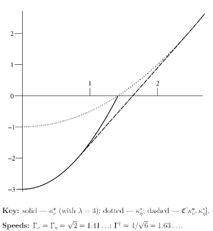
Figure 8.1: Illustration of how anomalous speed arises.

The point where each of them meets the horizontal axis gives the value of speed for that function. Thus, $\Gamma^{\dagger}$ exceeds the other two, which are both $\sqrt{2}$. Here $\Gamma^{\dagger}=4/\sqrt{6}$. In general, for $\lambda>1$, it is $(1+\lambda)/\sqrt{2\lambda}$, which can be made arbitrarily large by increasing $\lambda$ sufficiently.

9 Discussion of anomalous spreading

The critical function in Theorem 8.1 is $r={{\mathfrak{C}}[{\kappa}^{\ast\!\!\!\circ}_{\nu},{\kappa}^{\ast}_{\eta}]}^{{\circ}}$. Here is how it arises. The function ${\kappa}^{\ast\!\!\!\circ}_{\nu}$ describes the growth in numbers and spread of the type $\nu$. Conditional on these, ${\mathfrak{C}}[{\kappa}^{\ast\!\!\!\circ}_{\nu},{\kappa}^{\ast}_{\eta}]$ describes the growth and spread in expectation of those of type $\eta$. To see why this might be so, take a $b$ with ${\kappa}^{\ast\!\!\!\circ}_{\nu}(b)<0$ so that (3.5) describes the exponential growth of $Z^{(m)}_{\nu}[mb,\infty)$: there are roughly $\exp(-m{\kappa}^{\ast\!\!\!\circ}_{\nu}(b))$ such particles in generation $m$. Suppose now, for simplicity, that each of these produces a single particle of type $\eta$ at the parent’s position. As noted just before Theorem 3.2, the expected numbers of type $\eta$ particles in generation $r$ and in $[rc,\infty)$ descended from a single type $\eta$ at the origin is roughly $\exp(-r{\kappa}^{\ast}_{\eta}(c))$. Take $\lambda\in(0,1)$ with $m=\lambda n$ and $r=(1-\lambda)n$. Then, conditional on the development of the first $m$ generations, the expectation of the numbers of type $\eta$ in generation $n$ and to the right of $mb+rc=n(\lambda b+(1-\lambda)c)$ will be (roughly) at least $\exp(-n(\lambda{\kappa}^{\ast\!\!\!\circ}_{\nu}(b)+(1-\lambda){\kappa}^{\ast}_{\eta}(c)))$. As $b$, $c$ and $\lambda$ vary with $\lambda b+(1-\lambda)c=a$, the least value for $\lambda{\kappa}^{\ast\!\!\!\circ}_{\nu}(b)+(1-\lambda){\kappa}^{\ast}_{\eta}(c)$ is given by ${\mathfrak{C}}[{\kappa}^{\ast\!\!\!\circ}_{\nu},{\kappa}^{\ast}_{\eta}](a)$. There is some more work to do to show that this lower bound on the conditional expected numbers is also an upper bound—it is here that (8.1) comes into play. Finally, as indicated just before Theorem 3.2, this corresponds to actual numbers only when negative, so the positive values of this convex minorant are swept to infinity.

When the speed is anomalous, this indicative description of how $r={{\mathfrak{C}}[{\kappa}^{\ast\!\!\!\circ}_{\nu},{\kappa}^{\ast}_{\eta}]}^{{\circ}}$ arises makes plausible the following description of lines of descent with speed near $\Gamma^{\dagger}$. They will arise as a ‘dog-leg’, with the first portion of the trajectory, which is a fixed proportion of the whole, being a line of descent of type $\eta$ with a speed less than $\Gamma_{\eta}$. The remainder is a line of descent of type $\nu$, with a speed faster than $\Gamma_{\mu}$ (and also than $\Gamma^{\dagger}$).

Without the truncation, the linear operator approximating (near $u\equiv 1$) a $Q$ associated with a BRW describes the development of its expected numbers, and so it is tempting to define the speed using this, by looking at when expected numbers start to decay. In the irreducible case, Theorem 7.2 has an analogue for expected numbers, that

$$\frac{1}{n}\log\left(\mathbf{E}_{\nu}Z^{(n)}_{\sigma}[na,\infty)\right)\rightarrow-{\kappa}^{\ast}(a),$$

and so here the speed can indeed be found by looking at when expected numbers start to decay. In contrast, in the set up in Theorem 8.1

$$\frac{1}{n}\log\left(\mathbf{E}_{\nu}Z^{(n)}_{\eta}[na,\infty)\right)\rightarrow-{\mathfrak{C}}[{\kappa}^{\ast}_{\nu},{\kappa}^{\ast}_{\eta}](a),$$

and the limit here can be lower than ${\mathfrak{C}}[{\kappa}^{\ast\!\!\!\circ}_{\nu},{\kappa}^{\ast}_{\eta}]$—the distinction between the functions is whether or not positive values are swept to infinity in the first argument. Hence the speed computed by simply asking when expectations start to decay can be too large. In Figure 8.1, ${\mathfrak{C}}[{\kappa}^{\ast\!\!\!\circ}_{\nu},{\kappa}^{\ast}_{\eta}]$ is the same as ${\mathfrak{C}}[{\kappa}^{\ast}_{\nu},{\kappa}^{\ast}_{\eta}]$, but it is easy to see, reversing the roles of ${{\kappa}^{\ast}_{\nu}}$ and ${{\kappa}^{\ast}_{\eta}}$, that ${\mathfrak{C}}[{\kappa}^{\ast\!\!\!\circ}_{\eta},{\kappa}^{\ast}_{\nu}]$ is the same as ${\kappa}^{\ast}_{\nu}$. Thus if $\eta$ could produce $\nu$, rather than the other way round, expectations would still give the speed $\Gamma^{\dagger}$ but the true speed would be $\Gamma_{\nu}(=\Gamma_{\eta})$.

The general case, with many classes, introduces a number of additional challenges (mathematical as well as notational). It is discussed in Biggins, (2009). The matrix of transforms now has irreducible blocks on its diagonal, corresponding to the classes, and their Perron–Frobenius eigenvalues supply the $\kappa$ for each class, as would be anticipated from §7. Here a flavour of some of the other complications. The rather strong condition (8.1) means that the spatial distribution of type $\eta$ daughters to a type $\nu$ mother is irrelevant to the form of the result. If convergence is assumed only for some $\theta>0$ rather than all this need not remain true. One part of the challenge is to describe when these ‘off-diagonal’ terms remain irrelevant; another is to say what happens when they are not. If there are various routes through the classes from the initial type to the one of interest these possibilities must be combined: in these circumstances, the function $r$ in (8.2) need not be convex (though it will be increasing). It turns out that the formula for $\Gamma^{\dagger}$, which seems as if it might be particular to the case of two classes, extends fully—not only in the sense that there is a version that involves more classes, but also in the sense that the speed can usually be obtained as the maximum of that obtained using (8.4) for all pairs of classes where the first can have descendants in the second (though the line of descent may have to go through other classes on the way).

References

- Abért and Virág, (2005) Abért, M., and Virág, B. 2005. Dimension and randomness in groups acting on rooted trees. J. Amer. Math. Soc., 18(1), 157–192.
- Addario-Berry and Reed, (2009) Addario-Berry, L., and Reed, B. 2009. Minima in branching random walks. Ann. Probab., 37(3), 1044–1079.
- Alsmeyer and Iksanov, (2009) Alsmeyer, G., and Iksanov, A. 2009. A log-type moment result for perpetuities and its application to martingales in supercritical branching random walks. Electron. J. Probab., 14(10), 289–312.
- Alsmeyer and Rösler, (2006) Alsmeyer, G., and Rösler, U. 2006. A stochastic fixed point equation related to weighted branching with deterministic weights. Electron. J. Probab., 11(2), 27–56.
- Bachmann, (2000) Bachmann, M. 2000. Limit theorems for the minimal position in a branching random walk with independent logconcave displacements. Adv. in Appl. Probab., 32(1), 159–176.
- Biggins, (1976a) Biggins, J. D. 1976a. The first- and last-birth problems for a multitype age-dependent branching process. Adv. in Appl. Probab., 8(3), 446–459.
- Biggins, (1976b) Biggins, J. D. 1976b. Asymptotic Properties of the Branching Random Walk. D.Phil thesis, University of Oxford.
- Biggins, (1977a) Biggins, J. D. 1977a. Chernoff’s theorem in the branching random walk. J. Appl. Probab., 14(3), 630–636.
- Biggins, (1977b) Biggins, J. D. 1977b. Martingale convergence in the branching random walk. J. Appl. Probab., 14(1), 25–37.
- Biggins, (1995) Biggins, J. D. 1995. The growth and spread of the general branching random walk. Ann. Appl. Probab., 5(4), 1008–1024.
- Biggins, (1997) Biggins, J. D. 1997. How fast does a general branching random walk spread? Pages 19–39 of: Athreya, K. B., and Jagers, P. (eds), Classical and Modern Branching Processes (Minneapolis, MN, 1994). IMA Vol. Math. Appl., vol. 84. New York: Springer-Verlag.
- Biggins, (1998) Biggins, J. D. 1998. Lindley-type equations in the branching random walk. Stochastic Process. Appl., 75(1), 105–133.
- Biggins, (2009) Biggins, J. D. 2009. Spreading Speeds in Reducible Multitype Branching Random Walk. Submitted.
- Bramson, (1978a) Bramson, M. D. 1978a. Maximal displacement of branching Brownian motion. Comm. Pure Appl. Math., 31(5), 531–581.
- Bramson, (1978b) Bramson, M. D. 1978b. Minimal displacement of branching random walk. Z. Wahrscheinlichkeitstheorie verw. Gebiete, 45(2), 89–108.
- Bramson, (1983) Bramson, M. D. 1983. Convergence of solutions of the Kolmogorov equation to travelling waves. Mem. Amer. Math. Soc., 44(285), iv+190.
- Bramson and Zeitouni, (2009) Bramson, M. D., and Zeitouni, O. 2009. Tightness for a family of recursion equations. Ann. Probab., 37(2), 615–653.
- Dekking and Host, (1991) Dekking, F. M., and Host, B. 1991. Limit distributions for minimal displacement of branching random walks. Probab. Theory Related Fields, 90(3), 403–426.
- Grey, (1974) Grey, D. R. 1974. Explosiveness of age-dependent branching processes. Z. Wahrscheinlichkeitstheorie verw. Gebiete, 28, 129–137.
- Hammersley, (1974) Hammersley, J. M. 1974. Postulates for subadditive processes. Ann. Probab., 2, 652–680.
- Hu and Shi, (2009) Hu, Y., and Shi, Z. 2009. Minimal position and critical martingale convergence in branching random walk and directed polymers on disordered trees. Ann. Probab., 37(2), 742–789.
- Kingman, (1973) Kingman, J. F. C. 1973. Subadditive ergodic theory. Ann. Probab., 1, 883–909. With discussion and response.
- Kingman, (1975) Kingman, J. F. C. 1975. The first birth problem for an age-dependent branching process. Ann. Probab., 3(5), 790–801.
- Koukiou, (1997) Koukiou, F. 1997. Directed polymers in random media and spin glass models on trees. Pages 171–179 of: Athreya, K. B., and Jagers, P. (eds), Classical and Modern Branching Processes (Minneapolis, MN, 1994). IMA Vol. Math. Appl., vol. 84. New York: Springer-Verlag.
- Lagarias and Weiss, (1992) Lagarias, J. C., and Weiss, A. 1992. The problem: two stochastic models. Ann. Appl. Probab., 2(1), 229–261.
- Lewis et al., (2002) Lewis, M. A., Li, B., and Weinberger, H. F. 2002. Spreading speed and linear determinacy for two-species competition models. J. Math. Biol., 45(3), 219–233.
- Li et al., (2005) Li, B., Weinberger, H. F., and Lewis, M. A. 2005. Spreading speeds as slowest wave speeds for cooperative systems. Math. Biosci., 196(1), 82–98.
- Liggett, (1985) Liggett, T. M. 1985. An improved subadditive ergodic theorem. Ann. Probab., 13(4), 1279–1285.
- Liu, (1998) Liu, Q. 1998. Fixed points of a generalized smoothing transformation and applications to the branching random walk. Adv. in Appl. Probab., 30(1), 85–112.
- Liu, (2000) Liu, Q. 2000. On generalized multiplicative cascades. Stochastic Process. Appl., 86(2), 263–286.
- Lui, (1989a) Lui, R. 1989a. Biological growth and spread modeled by systems of recursions, I: mathematical theory. Math. Biosci., 93(2), 269–295.
- Lui, (1989b) Lui, R. 1989b. Biological growth and spread modeled by systems of recursions, II: biological theory. Math. Biosci., 93(2), 297–311.
- Mahmoud, (1992) Mahmoud, H. M. 1992. Evolution of Random Search Trees. Wiley-Intersci. Ser. Discrete Math. Optim. New York: John Wiley & Sons.
- McDiarmid, (1995) McDiarmid, C. 1995. Minimal positions in a branching random walk. Ann. Appl. Probab., 5(1), 128–139.
- Mollison and Daniels, (1993) Mollison, D., and Daniels, H. 1993. The “deterministic simple epidemic” unmasked. Math. Biosci., 117(1-2), 147–153.
- Peyrière, (2000) Peyrière, J. 2000. Recent results on Mandelbrot multiplicative cascades. Pages 147–159 of: Bandt, C., Graf, S., and Zähle, M. (eds), Fractal Geometry and Stochastics, II (Greifswald/Koserow, 1998). Progr. Probab., vol. 46. Basel: Birkhäuser.
- Weinberger, (1982) Weinberger, H. F. 1982. Long-time behavior of a class of biological models. SIAM J. Math. Anal., 13(3), 353–396.
- Weinberger, (2002) Weinberger, H. F. 2002. On spreading speeds and traveling waves for growth and migration models in a periodic habitat. J. Math. Biol., 45(6), 511–548.
- Weinberger et al., (2002) Weinberger, H. F., Lewis, M. A., and Li, B. 2002. Analysis of linear determinacy for spread in cooperative models. J. Math. Biol., 45(3), 183–218.
- Weinberger et al., (2007) Weinberger, H. F., Lewis, M. A., and Li, B. 2007. Anomalous spreading speeds of cooperative recursion systems. J. Math. Biol., 55(2), 207–222.