The Eastern Filament of W50

Abstract

We present new spectral (FPI and long-slit) data on the Eastern optical filament of the well known radionebula W50 associated with SS433. We find that on sub-parsec scales different emission lines are emitted by different regions with evidently different physical conditions. Kinematical properties of the ionized gas show evidence for moderately high ($V\sim 100\,~{}\rm km~{}s^{-1}\/$) supersonic motions. [O III]$\lambda$5007 emission is found to be multi-component and differs from lower-excitation [S II]$\lambda$6717 line both in spatial and kinematical properties. Indirect evidence for very low characteristic densities of the gas ($n\sim 0.1~{}\rm cm^{-3}\/$) is found. We propose radiative (possibly incomplete) shock waves in low-density, moderately high metallicity gas as the most probable candidate for the power source of the optical filament. Apparent nitrogen over-abundance is better understood if the location of W50 in the Galaxy is taken into account.

1 Introduction

W50 radionebula was first catalogued in the work by Westerhout (1958) and classified as a radiative-stage supernova remnant by Holden & Caswell (1969). However, the nebula is strongly affected by the activity of the central source SS433 (see Dubner et al. (1998) for review). It is not evident whether the contribution from the initial supernova explosion, that probably precursed formation of the compact accretor in SS433 system, may be distinguished from the impact of the jet and wind activity of the central system. Most of the peculiarities of W50 may be attributed to the jet activity of SS433. The total power of the jets is of the order $10^{39}\,~{}\rm erg~{}s^{-1}\/$. The jets are an immense source of energy capable to provide the energy of $\sim 10^{51}\,\rm erg$ characteristic for a usual supernova remnant (SNR) in about $3\times 10^{4}\,~{}\rm yr\/$, that is at least several times lower than the observed dynamical age of W50 (Yamamoto et al. 2008).

The morphology and radio properties of the nebula are fairly reproduced in numerical simulations with the preceeding SNR (Zavala et al. 2008; Velázquez & Raga 2000). However, it is not clear whether the central, quasi-spherical part of the radionebula requires a preceeding SNR cavity or not. The simulations also do not consider the possible emission of the warm gas that may appear in some parts of the nebula where the density is high enough for the shocked material to cool.

Warm gas in W50 was detected by Kirshner & Chevalier (1980) as the Eastern and the Western filaments. Recent investigation by (Boumis et al. 2007) proved that warm gas emission is present in different parts of the nebula but peaks in several bright optical filaments offset from the areas bright in X-ray and radio ranges.

The W50 optical filaments are distinguished among the known shell-like and SNR-like nebulae by the strong [N II] lines that were attributed by Zealey et al. (1980) to low velocity shocks and by Shuder et al. (1980) to nitrogen over-abundance. In this article, we analyse the reasons for the apparent nitrogen over-abundance, involving Galactic abundance gradients (see §4.1 for details).

In the next section we describe the observational material and the methods used for data reduction. In § 3 main results are presented. The results are discussed in § 4.

2 Observations and data reduction

All the observations were carried out in the prime focus of the Russian Special Astrophysical Observatory 6m telescope with the SCORPIO multi-mode focal reducer (Afanasiev & Moiseev 2005) and EEV 42-40 $2048\times 2048$ CCD.

The observational data summary is given in Table 1. Exposure times in the table are presented as the duration of a single exposure multiplied by the number of exposures or (for FPI data) the number of exposures in a single datacube multiplied by the number of datacubes.

Table 1: Observational logs for the long-slit and FPI data. Free spectral range is given for FPI data in the “spectral range” column.

	Long Slit		FPI
	Object	Background	[S II]$\lambda$6717	[O III]$\lambda$5007
Date	2006 Jul 31		2008 Jul 23
Disperser	VPHG550G		FPI501
Spectral Resolution $\delta v$,  $\rm km~{}s^{-1}\/$	500$\div$1000		31	36
Spectral Range, $\mathrm{\AA}$	3600$\div$7300		6717$\pm$7	5007$\pm$4
Seeing,	1.7		1.5$\div$2.2
Exposure Time, s	900$\times$4	600	120$\times$36$\times$2	200$\times$36
Position Angle, $\deg$	37		128 and -20	-20

2.1 Long-slit data

We use archival long-slit spectra of the brightest part of the Eastern filament. The slit was centered on the coordinates $\alpha=19^{h}14^{m}18^{s}$, $\delta=+5^{\circ}03^{\prime}20\arcsec{\,}$ (J2000). This position corresponds roughly to the center of the brightest part of the Eastern optical filament of W50 (Zealey et al. 1980) and is offset from the X-ray bright lens-shaped region (Brinkmann et al. 2007) by about 5^′ to the North. The length of the slit is about 5 arcminutes that is comparable to the length of the filament itself. This makes it difficult to subtract the background spectrum, therefore we use night sky exposures obtained the same night near the spectral standard star LDS 749B.

The position angle allows to trace the brightest regions of the filament, better visible in low excitation lines like [S II]$\lambda$6717.

2.2 Long-slit data reduction

Long slit data were reduced using IDL-based software. The reduction process includes all the standard reduction steps. Additionally, error frames are calculated in the assumption that the statistics is Poissonian for the quanta detected by the CCD. Spectral standard star LDS749B observed the same night in a 1^′ annular aperture is a standard from the list given by Turnshek et al. (1990). $4\times 4$ binning was used to reduce the readout noise. The reduction process for the night sky exposure was identical to that used for the object exposures. We also used an auxiliary image in the V band with the same coordinates and position angle to determine the coordinates of the field stars (see appendix A for details).

A significant complication for obtaining high a quality nebular spectrum is in the large number of field stars. We extract the spectra of 20 stars roughly brighter than 21${}^{\rm m}\!\!\,\,$ in V. Stellar spectra subtraction procedure is described in appendix A. After subtracting the contribution from the field stars, the two-dimensional nebular spectrum still contains some contribution from non-resolved stellar background. In addition to that, the stellar spectra were catalogued together with the approximate (accuracy about 1$\arcsec{\,}$) coordinates. We briefly discuss the field star spectra in appendix A.

Emission line profiles were fitted by gaussian and multi-gaussian models. The flux ratios of [N II]$\lambda\lambda$6548,6583 and [O III]$\lambda\lambda$4959,5007 doublets were fixed. We also assume the line-of-sight velocities and the widths of doublet components are equal. Kinematical information is difficult to study using long-slit spectra having low spectral resolution. However, it is possible to exclude emission line broadening by hundreds of  $\rm km~{}s^{-1}\/$ or more.

2.3 Scanning FPI data

We used a scanning Fabry-Pérot Interferometer (FPI) providing spectral resolution $30\div 35$ $\rm km~{}s^{-1}\/$ to study the kinematics of the same region. FPI field has a field of view close to 5^′ in diameter and was centered at $\alpha=19^{h}14^{m}25^{s}$, $\delta=+5^{\circ}03^{\prime}12\arcsec{\,}$ (J2000). The object was observed in two emission lines: $[{S\textsc{II}}]\lambda$6717 (total exposure $120\rm\,s\times 36$ spectral channels for each of the two datacubes) and $[{O\textsc{III}}]\lambda$5007 (total exposure $200{\rm\,s}\times 36$ spectral channels). The two datacubes obtained for the [S II] line differ in position angle that allows to eliminate ghosts from both the bright stars and the nebula itself (Moiseev & Egorov 2008). In the case of the [O III] datacube we also use lower quality data obtained during the next night, July 24, to remove the ghosts. The free spectral range was $13.7$ and $7.7$Å for $[{S\textsc{II}}]\lambda$6717 and $[{O\textsc{III}}]\lambda$5007, correspondingly.

Data reduction was performed in IDL environment. FPI data were reduced using ifpwid software designed by Alexei Moiseev. Data reduction algorithms are described by Moiseev (2002) and Moiseev & Egorov (2008). Line profile parameters were determined by fitting with Voigt functions of fixed Lorentzian widths ($31$ $\rm km~{}s^{-1}\/$ for [O III]$\lambda$5007 and $36$ $\rm km~{}s^{-1}\/$ for [S II]$\lambda$6717). Instrumental profile was measured using the spectra of a He-Ne-Ar calibration lamp. Voigt fitting procedure allows to measure line widths even when they are less than the instrumental profile width (Moiseev & Egorov 2008). Profiles were fitted only in the pixels where flux exceeded 20 ADU (corresponding to $S/N\sim 3$ for a given spatial sampling element). All the line-of-sight velocities presented here are heliocentric.

Several relatively bright stars were used for relative astrometry between the datacubes. Accuracy is at least better than the actual seeing (about $2\arcsec{\,}$).

3 Results

3.1 Integral spectrum

The integral spectrum obtained by simple integration along the $\sim 5^{\prime}$ slit is shown in Fig. 1. Night sky background was subtracted using a free multiplication factor (to account approximately for possible night sky lines variability) adjusted to accurately zero the [O I]$\lambda$5577 night sky emission in the residual spectrum.

However, the SS433+W50 system is located at a very low Galactic latitude ($b\simeq-2^{\circ}$). Even after removing 20 field stars and night sky emission line spectrum there is still a contribution from the Galactic unresolved background. For comparison, in Fig. 1 we show a stellar population model from Bruzual & Charlot (2003) with $T=12\,~{}\rm Gyr\/$ and 1.6$Z_{\odot}$ metallicity, reddened by $A_{\mathrm{V}}=2^{\rm m}\!\!\,\,$ (reddening curve by Cardelli et al. (1989) with $R_{\mathrm{V}}=3.1$). This interstellar absorption value was estimated by $\chi^{2}$-minimization technique for a fixed population age and metallicity, the latter chosen in consistence with the nebula position in the Galaxy (see § 4.1). The low interstellar absorption value (compared to the $\sim 4^{\rm m}\!\!\,\,$ value given below) may be due to the large number of unresolved stars in front of the filament (see appendix A).

Figure 1: The integral spectrum of W50 extracted from the long-slit data. Stellar population model spectrum shifted by 10${}^{-14}~{}\rm erg~{}cm^{-2}~{}s^{-1}\/$ down is shown for comparison (see text for details) by a dotted line.

Table 2: Optical emission line spectrum integrated over the long slit.

Line	F, 10${}^{-14}~{}\rm erg~{}cm^{-2}~{}s^{-1}\/$	F/F(H$\beta$)	F, 10${}^{-13}~{}\rm erg~{}cm^{-2}~{}s^{-1}\/$	F/F(H$\beta$)
			( Unreddened by $4^{\rm m}\!\!\,\,$ )
[O II]$\lambda$3727	15$\pm$1	3.16$\pm$0.26	360$\pm$30	10.83$\pm$0.91
[Ne III]$\lambda$3869	6.2$\pm$0.6	1.35$\pm$0.12	130$\pm$10	3.96$\pm$0.42
He II$\lambda$4686	0.8$\pm$0.11	0.18$\pm$0.02	7.2$\pm$1.0	0.21$\pm$0.03
H$\beta$	4.6$\pm$0.3	1.00$\pm$0.06	34$\pm$2	1.00$\pm$0.06
[O III]$\lambda$4959	9.6$\pm$0.1	2.09$\pm$0.02	59.3$\pm$0.7	1.77$\pm$0.02
[O III]$\lambda$5007	28.8$\pm$0.3	6.26$\pm$0.07	178$\pm$2	5.30$\pm$0.06
[N I]$\lambda$5200	3.9$\pm$0.2	0.84$\pm$0.04	19.3$\pm$0.9	0.58$\pm$0.03
[N II]$\lambda$5755	1.7$\pm$0.2	0.38$\pm$0.05	5.1$\pm$0.6	0.15$\pm$0.02
[O I]$\lambda$6300	107.6$\pm$1.0	23.42$\pm$0.21	210$\pm$2	6.27$\pm$0.05
[O I]$\lambda$6363	35.9$\pm$0.3	7.81$\pm$0.07	70.1$\pm$0.6	2.09$\pm$0.02
[N II]$\lambda$6548	45$\pm$5	9.81$\pm$1.16	73$\pm$9	2.18$\pm$0.26
H$\alpha$	58$\pm$5	12.63$\pm$1.19	96$\pm$9	2.86$\pm$0.27
[N II]$\lambda$6583	135$\pm$6	29.42$\pm$1.33	219$\pm$10	6.53$\pm$0.29
[S II]$\lambda$6717	55$\pm$3	11.87$\pm$0.61	81$\pm$4	2.41$\pm$0.13
[S II]$\lambda$6731	36$\pm$3	7.76$\pm$0.60	53$\pm$4	1.58$\pm$0.13
[Ar III]$\lambda$7135	7.4$\pm$0.2	1.60$\pm$0.05	8.5$\pm$0.3	0.25$\pm$0.01

Integral line fluxes are given in Table 2. Several emissions are detected for the first time. The most interesing among these is the He II$\lambda$4686 line. Though its profile may be affected by the stellar population spectrum, the line is clearly identified. The measured He II$\lambda$4686 / H$\beta$ intensity ratio is as high as 0.2 that is likely to be the consequence of high electronic temperature. Line profile may be however affected by the stellar background, therefore the uncertainty of its flux may be larger than the proposed 15% statistical uncertainty given in Table 2.

Assuming that the temperature of the warm gas is $T_{e}\simeq 15\,000\,\rm K$, and the density is lower than $\sim$10  $\rm cm^{-3}\/$, one may estimate the intrinsic H$\alpha$ / H$\beta$ intensity ratio as 2.85 (Osterbrock & Ferland 2006). Interstellar absorption may be therefore estimated (applying reddening curve by Cardelli et al. (1989)) by the following formula:

$$A_{\mathrm{V}}\simeq 0.15\lg\left(\frac{F(H\alpha)/F(H\beta)}{2.85}\right)$$ (1)

Interstellar absorption is affected by the still poorly known contribution from the stellar background. If no H$\beta$ absorpion is present, $A_{\mathrm{V}}=4^{\rm m}\!\!.\,0\pm 0.2$. If the best-fit stellar population model (see above) is subtracted, $A_{\mathrm{V}}\simeq 3^{\rm m}\!\!.\,5$. Equivalent widths of higher-order absorption lines H$\gamma$ and H$\delta$ are definitely over-estimated by the stellar population model (see figure 1), maybe because brighter stars of intermediate spectral classes were cleaned from the spectrum. The systematic absorption shift produced by the unresolved fore- and background stars is therefore no more than $\sim 0^{\rm m}\!\!.\,5$ that is comparable to the absorption variation along the slit (see section 4.3). For the lines at the blue end of the spectrum (namely, for [O II]$\lambda$3727) it introduces an $\sim 2$ uncertainty.

We estimate the characteristic intensity ratios of [S II] and [N II] lines as I([S II]$\lambda$6717) / I([S II]$\lambda$6731) = 1.52$\pm$0.22 and (I([N II]$\lambda$6583) + I([N II]$\lambda$6548) / I([S II]$\lambda$5755) = 58$\pm$15, correspondingly. Applying TEMDEN internet service (http://stsdas.stsci.edu/nebular/temden.html, see Shaw & Dufour (1994) for calculation algorythm description) allows to estimate the electron temperature as $T_{e}=13\,000\pm 2\,000\,\rm K$. Electron density is too low to measure it via [S II] lines. Sulfur lines give only an upper limit, $n_{\mathrm{e}}\lesssim 100\,~{}\rm cm^{-3}\/$. Note that these diagnostic lines are emitted in rather dense regions of the nebula. Probably, the real electron density is by two-three orders of magnitude lower than this, see § 4.2.

3.2 Kinematics

Kinematical properties, as well as the morphology of the filament, differ for the [S II] and [O III] emissions. The fine subparsec-scale structure of the filament (that is still much coarser than the actual seeing) is present for the low-ionisation sulfur line but not for [O III]$\lambda$5007. Most probably, the [S II]$\lambda$6717 line is emitted by denser inner parts of the filamentary structure while the outer, hotter and more rarefied layers are better visible in higher-ionization lines. The picture is similar to the shocked cloud structure in radiative-stage SNRs. We show the two intensity maps and several selected line profiles in Fig. 3. The 56  $\rm km~{}s^{-1}\/$ mark corresponds to the line-of-sight velocity reported by Boumis et al. (2007) as the systemic velocity.

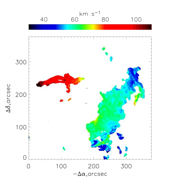
Figure 2: Velocity map for [S II]$\lambda$6717.

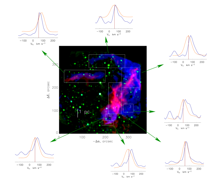
Figure 3: The two intensity maps overlapped. [S II]$\lambda$6717 intensity is shown by red, [O III]$\lambda$5007 by blue (grayscale and dotted contours in the black&white version, dotted lines are logarythmically spaced by a factor of 10). For seven regions of interest line profiles are also given (red/dotted for [S II] and blue/solid for [O III]). The vertical line everywhere has the velocity of 56 $\rm km~{}s^{-1}\/$.

The velocity map for [S II]$\lambda$6717 is given in Fig. 2. The brighter part of the filament shows practically constant line-of-sight velocity of 50$\div$70  $\rm km~{}s^{-1}\/$ with about 20  $\rm km~{}s^{-1}\/$ variations near the bubble structure covered by regions 0 and 1 in Fig. 3. The line is broader than the components of [O III] and is generally broadened by 15$\div$20  $\rm km~{}s^{-1}\/$. In the regions 1 and 6 the line has larger velocity dispersion of about 40  $\rm km~{}s^{-1}\/$. The most outstanding feature is the longitudally oriented smaller filament (region 2 in Fig. 3). It is evidently kinematically shifted from the main body of the filament. Its line-of-sight velocity is in the range of 80$\div$100  $\rm km~{}s^{-1}\/$.

The profiles of [O III]$\lambda$5007, on the other hand, show more complicated structure. In most of the regions of interest two to four components with velocity dispersion about 10  $\rm km~{}s^{-1}\/$ are present: the brighter one at 70$\div$80  $\rm km~{}s^{-1}\/$, slightly shifted with respect to the sulfur line, one at 120$\div$130  $\rm km~{}s^{-1}\/$ and blueward-shifted components at -10$\div$0 and -80$\div$-100  $\rm km~{}s^{-1}\/$.

4 Discussion

4.1 Abundances

The crucial point in understanding the emission line spectrum of the nebula is in the distance towards the Galactic center. Let us assume the distance from the Sun is $5\div 6\,~{}\rm kpc\/$ (Lockman et al. 2007). The Galactic latitude and longitude are equal to $b=-2^{\circ}.3$ and $l=39^{\circ}.8$, correspondingly, and the distance from the Sun towards the Galactic center $7.5\div 8.5\,~{}\rm kpc\/$ (see for example Eisenhauer et al. (2003) and references therein). We come to the conclusion that SS433 and W50 are situated at a Galactocentric distance of about $4\div 5\,~{}\rm kpc\/$, i. e., at least $3\,~{}\rm kpc\/$ closer to the center than the Sun. That suggests the metallicity of the gas should be somewhat higher than solar. Using the Galactic abundance gradient values given by Alibés et al. (2001), one may estimate the oxygen abundance as ${\rm[O/H]}\simeq 0.1\div 0.2$ (relative to the Solar value). For nitrogen the enrichment may be as high as ${\rm[N/H]}\simeq 0.2\div 0.3$ because its abundance scales non-linearly with metallicity and its gradients are generally steeper at higher metallicities (van Zee 1998). Here we consider “solar” abundances $12+\lg{\rm O/H}=8.7$ and $12+\lg{\rm N/H}=7.9$ according to Grevesse & Sauval (1998).

High ambient metallicity makes the unordinary spectrum of W50 more reasonable. In a solar metallicity environment, [N II]$\lambda$6583 over H$\alpha$ intensity ratio for a W50 analogue is likely to be $\sim 1$. Together with the oxygen line intensity ratios $[{O\textsc{I}}]\lambda 6300/[{O\textsc{III}}]\lambda 5007\sim 1$ and $[{O\textsc{II}}]\lambda 3727/[{O\textsc{III}}]\lambda 5007\sim 2$ it makes the filament a bona fide shock-powered nebula (Baldwin et al. 1981). The observed $[{O\textsc{III}}]\lambda 5007/{\rm H}\beta\sim 5$ ratio is also quite reasonable, if high ambient metallicity is taken into account.

Some high ionization features like the He II$\lambda$4686 emission (and still high [N II], [O III] and [Ne III] line intensities) may be attributed to incompleteness of the shock waves. Though cooling time is short enough for the observed shock waves to radiate most of their energy, they may still remain incomplete (i. e., lack lower-temperature gas) if additional energy sources such as X-ray and EUV radiation from SS433 or X-ray bright regions of the nebula are present. Shock multiplicity also restricts the sizes of cooling regions. It should be also noted that the spatial cooling region scale is much larger than the projected width of the long slit, therefore the nebular regions traced by the slit may represent gas temperatures in unequal proportions. Due to all these reasons, shocks in W50 may bear incompleteness signatures even though their cooling times are considerably shorter than the age of the nebula.

4.2 Kinematical structure

Different kinematical behaviour of the two forbidden emissions may be explained qualitatively by a system of moderately fast (from tens to $\sim 100\,~{}\rm km~{}s^{-1}\/$) shock waves. Large-scale turbulent motions in recently shocked gas are transformed into microturbulent motions in cooler gas emitting the [S II]$\lambda$6717 line that has significantly lower ionisation potential. Due to this reason, several velocity components transform into general line broadening (lower-velocity motions at smaller spatial scales) for lower ionisation lines.

Spatial displacement between the regions emitting in the two lines is mostly of the order arcseconds, up to $10\div 20\arcsec{\,}$. That gives (if we assume that the spatial structure reflects gas cooling behind shock fronts) approximate cooling region width $\sim 0.1\div 1\,~{}\rm pc\/$. This range may be used to estimate the density of the shocked gas. If the matter moves with velocity $u$ (presumably the same order with the shock front velocity), it cools from $T_{2}$ temperature to $T_{1}$ at the lengthscale:

$$l\simeq\frac{u(T_{2}-T_{1})}{n_{\mathrm{e}}\Lambda}$$

Here $n_{\mathrm{e}}$ is electron density, and $\Lambda$ is cooling function. $n_{\mathrm{e}}$ may be estimated from the observational data, if $l$ and $u$ are known. Cooling function $\Lambda\sim 10^{-21}\div 10^{-22}\,\rm erg\,cm^{-3}\,s^{-1}$ for $T\sim(1\div 1.5)\times 10^{4}\,\rm K$, hence:

$$\begin{array}[]{l}n_{\mathrm{e}}\sim 0.1\left(\frac{u}{100\,~{}\rm km~{}s^{-1}\/}\right)\left(\frac{T}{10^{4}\,\rm K}\right)\left(\frac{l}{0.5\,~{}\rm pc\/}\right)^{-1}\times\\ \qquad{}\times\left(\frac{\Lambda}{10^{-22}\,\rm erg\,cm^{-3}\,s^{-1}}\right)^{-1}~{}\rm cm^{-3}\/\\ \end{array}$$

Gas density is therefore likely to be well below the lower limits set by the [S II] doublet estimates (see §3.1). The corresponding cooling timescale is $\sim l/u\sim 500\,~{}\rm yr\/$ that is significantly lower than the proposed age of the nebula.

The Eastern optical filament is powered by shock waves with $V\sim 100~{}\rm km~{}s^{-1}\/$. This characteristic velocity is in good agreement with the value given by Boumis et al. (2007) for the expansion velocity of the nebula. The motions seem to be chaotic and may be the result of the post-shock turbulence of stronger shock waves that produce the X-ray emission in X-ray bright regions of W50 (Brinkmann et al. 2007). Brinkmann et al. (2007) do not provide any shock velocity estimates, but they estimate the thermal component temperature as $T\sim 0.2\,~{}\rm keV\/$, that yields $T_{S}\sim 400\,~{}\rm km~{}s^{-1}\/$ for Sedov solution (see Hamilton et al. (1983)). Strong radiative shock waves are predicted to produce supersonic turbulence with average Mach number $\sim 0.2\mathcal{M}$, where $\mathcal{M}$ is the upstream Mach number of the primary shock (Folini & Walder 2006). For an isothermal primary shock, that means also a factor of 5 decrease of the characteristic velocity. That approximately accounts for the observed velocity scales present in W50 (except for the jet velocity itself) as well as for the fine structure formation itself.

Otherwise, the moderate power shocks may trace the expansion of the gas heated in the bow-shock of the Eastern jet. Thermal velocity in the gas that emits the observed X-ray radiation ($T\sim 0.2\,~{}\rm keV\/$, see above) is of the order $\sim 100\div 200~{}\rm km~{}s^{-1}\/$, that directly yields the required velocity scale. A pressure-driven shell solution (Castor et al. 1975) produced by a power source $L\sim 10^{39}~{}\rm erg~{}s^{-1}\/$ and expanding into ISM with $n\sim 1\,~{}\rm cm^{-3}\/$ will have expansion velocity:

$$\begin{array}[]{l}V\simeq 0.6K^{5/3}\left(\frac{L}{\rho}\right)^{3/5}R^{-2/3}\simeq\\ \simeq 100\left(\frac{L}{10^{39}~{}\rm erg~{}s^{-1}\/}\right)^{1/3}\left(\frac{n}{1~{}\rm cm^{-3}\/}\right)^{-1/3}\times\\ \qquad{}\qquad{}\times\left(\frac{R}{50~{}\rm pc\/}\right)^{-2/3}~{}\rm km~{}s^{-1}\/\\ \end{array}$$

Here, $K\simeq 0.76$ is a dimensionless constant. If the expansion of W50 is fed by the power of the relativistic jets, it is likely to have characteristic velocities similar to the observed $V\sim 100\,~{}\rm km~{}s^{-1}\/$. However, it is difficult to interpret the observed velocity components as the two walls of a single shell. Expansion should proceed in a more complicated way than spherically-symmetric bubble expansion.

4.3 Absorption gradients

SS433 and W50 are not only heavily absorbed, but the absorption itself is patchy, from about 8^m for the central object towards $\lesssim 4^{m}$ for some parts of the Eastern filament. Variable absorption is important for the observed morphology of the filaments on the scales larger than minutes (Boumis et al. 2007).

In figure 4 we show the V-band absorption calculated using the long-slit data devided into 10 bins. For each, we performed the procedure identical to this made for the integral spectrum in section 3.1. Error bars are 1$\sigma$ approximation uncertainties. $A_{V}$ changes by about $0^{\rm m}\!\!.\,5$, and therefore may be responsible for about 50% flux variations for lines near $5000\mathrm{\AA}$. In contrast, emission line intensities along the slit vary by about an order of magnitude.

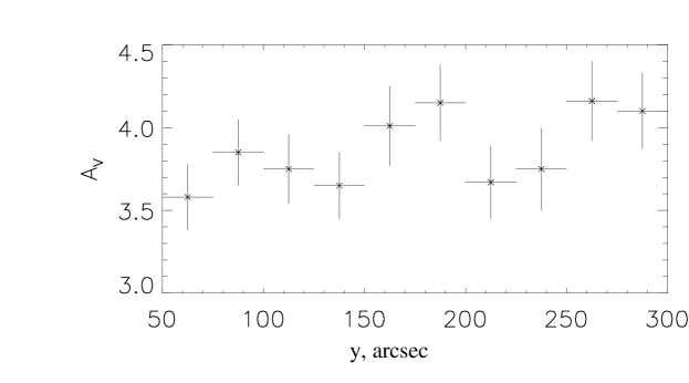
Figure 4: Spatially-resolved V-band interstellar absorption as function of coordinate along the slit

Variations induced by variable absorption hardly affect the morphology in emission lines. Firstly because the observed fluxes are definitely linked with kinematics (see § 3.2). Besides this, in regions of very low [S II] fluxes we observe bright emission in the [O III] line, that is possible only due to physical reasons. Last but not least, the bright regions covered by the long slit do not have absorption much lower than the fainter parts of the filament.

5 Conclusions

We come to the conclusion that the optical filaments of W50 are mainly powered by shocks with velocities of the order 100$\div$200 $\rm km~{}s^{-1}\/$ and less. Flows with line-of-sight velocities differing by $\pm$100 $\rm km~{}s^{-1}\/$ are detected in the [O III]$\lambda$5007 emission line produced in the recently shocked, relatively hot gas. For lower-ionisation lines kinematics is different: we detect only general broadening of the [S II] line. Probably, cooler gas shows both lower turbulent velocities and larger number of velocity components. We also find at least two spatially resolved shock fronts in the FPI field of view propagating in different directions. Their line-of-sight velocities differ by about 50 $\rm km~{}s^{-1}\/$. Our results are compolementary to the results reported by Boumis et al. (2007) and provide more detailed picture of a smaller part of the nebula.

The optical emission-line spectrum of W50 Eastern filament bears the main signatures of a radiative (possibly, incomplete) shock such as enhanced collisionly excited lines of different ionization potentials. The observed gas shows a broad range of physical properties. In general, the gas is rarefied ($n\sim 10^{-2}\div 1\,~{}\rm cm^{-3}\/$) and moderately over-abundant in oxygen and nitrogen. This apparent over-abundance is likely to be attributed to the high metallicity of the Galactic gas at the comparatively low ($\sim 4\div 5\,~{}\rm kpc\/$) distance from the Galactic center. Nitrogen lines are primarily affected because of stronger nitrogen gradient in the Galactic disc.

Appendix A Field Stars Spectroscopy

In order to obtain better integral long-slit spectrum, field stars were cleaned from the 2D-specta of the object and night sky background. Stars were identified automatically on spectrally-integrated one-dimensional images. Stellar profiles were approximated by Gaussian function (using Moffat function does not increase $\chi^{2}$ significantly but decreases stability of the algorythm) with parameters polynomially dependent on the wavelength.

20 field stars (roughly brighter than 21${}^{\rm m}\!\!\,\,$) were finally extracted from the object frame. To our knowledge, none of the stars are present in existing stellar catalogues. We suggest that the data may be of some use for future astrophysical applications. We identify the spectra automatically by $\chi^{2}$-fitting with spectral standards from STELIB (http://webast.ast.obs-mip.fr/stelib, see Le Borgne et al. (2003)) simultaneously estimating interstellar absorption (Cardelli et al. (1989) extinction curves with $R_{\mathrm{V}}=3.1$ were used). We summarize our results in Table 3. Spectral classes are given with accuracy about 1$\div$2 spectral subclasses. Spectral resolution does not allow to determine the luminosity class self-consistently, but we still give the best-fit luminosity classes. Coordinates are measured with accuracy $\sim 1\arcsec{\,}$ and given in J2000. Coordinates were measured by comparison of the auxiliary SCORPIO image (see § 2.2) to the Palomar Digitized Sky Survey image with correct astrometry. starast procedure written by W. Landsman was used to set the coordinate grid on the SCORPIO image and, subsequently, along the slit.

It is easy to check that most of the stars in the observed sector of the Galaxy and the relevant range of magnitudes should be foreground main sequence stars of the spectral classes from A to K. This is confirmed by the relatively low interstellar absorption for most of the stars. A $1\arcsec{\,}\times 300\arcsec{\,}$ slit covers about $3\times 10^{-8}$ of the Galactic volume, that should contain about 1000 main sequence stars, several white dwarfs and probably no giant and supergiant stars. If one considers only the nearest parsec of the volume and only the brightest stars (say, $M_{\mathrm{V}}\lesssim 5^{\rm m}\!\!\,\,$), their number should be of the order 10$\div$50. Most of the stars have visual magnitudes in the range $18\div 21^{\rm m}\!\!\,\,$. We do not however give the best-fit magnitude values because of the unkown slit losses.

Table 3: Field stars: spectral classes, best-fit interstellar absorption and coordinates.

	Spectral Class	$A_{v},\,^{\rm m}\!\!\,\,$	$\alpha$	$\delta$
1	G7 V	0.5	19h14m12${}^{s}\!\!$.0	+05∘05′08$\arcsec{\,}$
2	K0 V	1.5	19 14 18.0	+05 03 05
3	G9 III	2.2	19 14 17.2	+05 03 22
4	F2 V	2.8	19 14 22.1	+05 01 33
5	G9 III	3.2	19 14 13.2	+05 04 39
6	G0 V	0.9	19 14 18.5	+05 02 54
7	G8 V	3.8	19 14 22.4	+05 01 31
8	K0 V	0(?)	19 14 23.7	+05 01 07
9	K1 V	0.7	19 14 22.0	+05 01 41
10	K1 III	5.6	19 14 23.6	+05 01 09
11	K1 V	4.3	19 14 24.0	+05 01 03
12	G8 V	3.3	19 14 23.0	+05 01 23
13	G0 V	2.7	19 14 24.4	+05 00 49
14	G0 V	3.6	19 14 19.2	+05 02 35
15	K2 V	2.0	19 14 17.2	+05 03 13
16	K4 III	3.4	19 14 21.6	+05 01 41
17	K4 III	1.7	19 14 15.9	+05 03 45
18	G9 III	1.2	19 14 15.2	+05 04 00
19	G8 V	6.0	19 14 24.2	+05 00 56
20	A9 III	3.9	19 14 19.1	+05 02 43