Asymptotic zero distribution of multiple orthogonal polynomials associated with Macdonald functions

Lun Zhang111Department of Mathematics, Katholieke Universiteit Leuven, Celestijnenlaan 200B, B-3001 Leuven, Belgium. E-mail: lun.zhang@wis.kuleuven.be. , Pablo RomΓ‘n222Department of Mathematics, Katholieke Universiteit Leuven, Celestijnenlaan 200B, B-3001 Leuven, Belgium. E-mail: pablo.roman@wis.kuleuven.be.
Abstract

We study the asymptotic zero distribution of type II multiple orthogonal polynomials associated with two Macdonald functions (modified Bessel functions of the second kind). Based on the four-term recurrence relation, it is shown that, after proper scaling, the sequence of normalized zero counting measures converges weakly to the first component of a vector of two measures which satisfies a vector equilibrium problem with two external fields. We also give the explicit formula for the equilibrium vector in terms of solutions of an algebraic equation.

1 Introduction

Given a positive measure $\mu$ on the real line for which the support is not finite and all moments exist, there exists a sequence of monic orthogonal polynomials $\{p_{k}\}$ of degree $k$. Such polynomials satisfy a three-term recurrence relation of the form

$$xp_{k}(x)=p_{k+1}(x)+b_{k}p_{k}(x)+a_{k}^{2}p_{k-1}(x),\quad k\geq 0,$$ (1.1)

with $a_{k}\geq 0$, $b_{k}\in\mathbb{R}$ and $p_{0}\equiv 1$, $p_{-1}\equiv 0$.

It is well-known that the zeros of $p_{k}$ are real and simple. We can associate with $p_{k}(x)$ the normalized zero counting measure

$$\nu(p_{k})=\frac{1}{k}\sum_{j=1}^{k}\delta_{x_{j,k}},$$ (1.2)

where $x_{j,k}$, $j=1,\ldots,k$, are the zeros of $p_{k}$ and $\delta_{x}$ denotes the Dirac point mass at $x$. A measure $\nu$ is called the asymptotic zero distribution of $\{p_{k}\}$ if

$$\lim_{k\to\infty}\int f\,d\nu(p_{k})=\int f\,d\nu$$

for every bounded continuous function $f$ on $\mathbb{R}$, i.e., it is the weak limit of the measures $\nu(p_{k})$.

Suppose $\lim_{k\to\infty}a_{k}=a$ and $\lim_{k\to\infty}b_{k}=b$ with $a>0$ and $b\in\mathbb{R}$, then the polynomials generated by (1.1) have the asymptotic zero distribution $w_{[\alpha,\beta]}$ with density

$$\frac{dw_{[\alpha,\beta]}(x)}{dx}=\begin{cases}\frac{1}{\pi\sqrt{(\beta-x)(x-\alpha)}},&x\in[\alpha,\beta],\\ 0,&\text{elsewhere},\end{cases}$$ (1.3)

where $\alpha=b-2a$, $\beta=b+2a$; cf. [16].

This result has been extended in [15] to the case of orthogonal polynomials generated by the recurrence relation

$$xp_{k,n}(x)=p_{k+1,n}(x)+b_{k,n}p_{k,n}(x)+a_{k,n}^{2}p_{k-1,n}(x),\quad k,n\in\mathbb{N},$$

with varying recurrence coefficients $a_{k,n}>0$ and $b_{k,n}\in\mathbb{R}$ depending on a parameter $n$. Assume that the recurrence coefficients have continuous limits

limk/nβ†’sak,n=a​(s),limk/nβ†’sbk,n=b​(s),formulae-sequencesubscriptβ†’π‘˜π‘›π‘ subscriptπ‘Žπ‘˜π‘›π‘Žπ‘ subscriptβ†’π‘˜π‘›π‘ subscriptπ‘π‘˜π‘›π‘π‘ \lim_{k/n\to s}a_{k,n}=a(s),\quad\lim_{k/n\to s}b_{k,n}=b(s),

where $a:(0,\infty)\to[0,\infty)$, $b:(0,\infty)\to\mathbb{R}$ and the notation limk/nβ†’ssubscriptβ†’π‘˜π‘›π‘ \lim_{k/n\to s} means that both $k,n\to\infty$ with k/nβ†’s>0β†’π‘˜π‘›π‘ 0k/n\to s>0, it is proved that the asymptotic zero distribution is given by the average

limk/nβ†’sν​(pk,n)=1sβ€‹βˆ«0sw[α​(s),β​(s)]​𝑑s,subscriptβ†’π‘˜π‘›π‘ πœˆsubscriptπ‘π‘˜π‘›1𝑠superscriptsubscript0𝑠subscript𝑀𝛼𝑠𝛽𝑠differential-d𝑠\lim_{k/n\to s}\nu(p_{k,n})=\frac{1}{s}\int_{0}^{s}w_{[\alpha(s),\beta(s)]}ds, (1.4)

where α​(s):=b​(s)βˆ’2​a​(s)assign𝛼𝑠𝑏𝑠2π‘Žπ‘ \alpha(s):=b(s)-2a(s), β​(s):=b​(s)+2​a​(s)assign𝛽𝑠𝑏𝑠2π‘Žπ‘ \beta(s):=b(s)+2a(s) and $w_{[\alpha,\beta]}$ is defined by (1.3) if $\alpha<\beta$ and by $\delta_{\alpha}$ if $\alpha=\beta$; see Theorem 1.10 of [15].

A natural generalization of this case consists in considering, for each $n\in\mathbb{N}$, polynomials $P_{k,n}$ satisfying an $m$-term recurrence relation with varying coefficients:

$$xP_{k,n}(x)=P_{k+1,n}(x)+b_{k,n}^{(0)}P_{k,n}(x)+b_{k,n}^{(1)}P_{k-1,n}(x)+\cdots+b_{k,n}^{(m-2)}P_{k+2-m,n}(x),$$ (1.5)

where $P_{0}\equiv 1$, $P_{-1}\equiv 0,\ldots,P_{-m+2}\equiv 0$ and the recurrence coefficients have scaling limits

limk/nβ†’sbk,n(j)=b(j)​(s),j=0,…,mβˆ’2,formulae-sequencesubscriptβ†’π‘˜π‘›π‘ superscriptsubscriptπ‘π‘˜π‘›π‘—superscript𝑏𝑗𝑠𝑗0β€¦π‘š2\lim_{k/n\to s}b_{k,n}^{(j)}=b^{(j)}(s),\qquad j=0,\ldots,m-2,

for certain functions $b^{(0)},\ldots,b^{(m-2)}$.

For the simplest case $b_{k,n}^{(j)}=b^{(j)}(s)$, i.e., we remove the dependence on the parameter $n$ and the recurrence coefficients in (1.5) are actually constant, the zeros of $P_{k}=P_{k,n}$ are closely related to the spectrum of certain banded Toeplitz matrix. Indeed, if we associate with the functions $b^{(j)}$ a family of functions

$$A_{s}(z)=z+b^{(0)}(s)+b^{(1)}(s)z^{-1}+\cdots+b^{(m-2)}(s)z^{-m+2},$$ (1.6)

and the sequence of $k\times k$ Toeplitz matrices (Tk​(As))ksubscriptsubscriptπ‘‡π‘˜subscriptπ΄π‘ π‘˜(T_{k}(A_{s}))_{k} with symbol $A_{s}$, defined by

$$(T_{k}(A_{s}))_{jl}=\begin{cases}1,&\text{if }l=j+1,\\ b^{(i)}(s),&\text{if }l=j-i,\qquad i=0,\ldots,m-2,\\ 0,&\text{otherwise},\end{cases}$$ (1.7)

it is readily seen that $P_{k}(\lambda)=0$ if and only if $\lambda$ is an eigenvalue of $T_{k}(A_{s})$. Hence, the investigation of limiting zero distribution of $P_{k}$ is equivalent to the study of the limiting behavior of the spectrum of $T_{k}(A_{s})$ as $k\to\infty$.

The limiting behavior of the spectrum of $T_{k}(A_{s})$ as $k\to\infty$ is characterized by the solutions of the algebraic equation $A_{s}(z)=x$; see [3]. For every $x\in\mathbb{C}$, there exist exactly $m-1$ solutions of the equation $A_{s}(z)=x$ (assume that b(mβˆ’2)​(s)β‰ 0superscriptπ‘π‘š2𝑠0b^{(m-2)}(s)\neq 0), which we denote by $z_{j}(x,s)$, $j=1,\ldots,m-1$ and label these solutions by their absolute value so that

$$|z_{1}(x,s)|\geq|z_{2}(x,s)|\geq\cdots\geq|z_{m-1}(x,s)|>0.$$ (1.8)

We put

$$\Gamma_{1}(s)=\{x\in\mathbb{C}\mid|z_{1}(x,s)|=|z_{2}(x,s)|\},$$ (1.9)

which is a finite union of analytic arcs.

It was shown by Schmidt and Spitzer [20] that the eigenvalues of $T_{k}(A_{s})$ accumulate on the contour $\Gamma_{1}(s)$ as $k$ tends to $\infty$. Moreover, Hirschman [12] proved that the sequence of normalized counting measures of the eigenvalues of $T_{k}(A_{s})$ converges weakly to a Borel probability measure ΞΌ1ssubscriptsuperscriptπœ‡π‘ 1\mu^{s}_{1} supported on $\Gamma_{1}(s)$ as $k\to\infty$; see also [3, ChapterΒ 11]. The precise form of ΞΌ1ssubscriptsuperscriptπœ‡π‘ 1\mu^{s}_{1} is given by

d​μ1s​(x)=12​π​i​(z1βˆ’β€²β€‹(x,s)z1βˆ’β€‹(x,s)βˆ’z1+′​(x,s)z1+​(x,s))​d​x,𝑑subscriptsuperscriptπœ‡π‘ 1π‘₯12πœ‹π‘–subscriptsuperscript𝑧′limit-from1π‘₯𝑠subscript𝑧limit-from1π‘₯𝑠subscriptsuperscript𝑧′limit-from1π‘₯𝑠subscript𝑧limit-from1π‘₯𝑠𝑑π‘₯d\mu^{s}_{1}(x)=\frac{1}{2\pi i}\left(\frac{z^{\prime}_{1-}(x,s)}{z_{1-}(x,s)}-\frac{z^{\prime}_{1+}(x,s)}{z_{1+}(x,s)}\right)dx, (1.10)

which is due to the result in [10]. Here, we have that β€² denotes the derivative with respect to $x$, $dx$ is the complex line element on $\Gamma_{1}(s)$ and $z_{1\pm}(x,s)$ is the limiting value of $z_{1}(\tilde{x},s)$ as $\tilde{x}\to x$ from the $\pm$ side of $\Gamma_{1}(s)$. Moreover, the measure $\mu_{1}^{s}$ is also characterized by an equilibrium problem; see Theorem 2.2 below for a statement in the context of the specific example considered in this paper.

Under certain conditions, the polynomials $P_{k,n}$ satisfying the recurrence (1.5) have a limiting zero distribution as well, which is an average, with respect to the parameter $s$, of the measures (1.10). More precisely, we have (see Theorem 1.2 in [14]):

Theorem 1.1.

Let for each $n\in\mathbb{N}$, $m-1$ sequences $\{b_{k,n}^{(j)}\}_{k=0}^{\infty}$, $j=0,\ldots,m-2$, of real coefficients be given and assume that there exist continuous functions $b^{(j)}:[0,\infty)\to\mathbb{R}$, $j=0,\ldots,m-2$, such that for each $s\geq 0$,

limk/nβ†’sbk,n(j)=b(j)​(s),j=0,…,mβˆ’2.formulae-sequencesubscriptβ†’π‘˜π‘›π‘ subscriptsuperscriptπ‘π‘—π‘˜π‘›superscript𝑏𝑗𝑠𝑗0β€¦π‘š2\lim_{k/n\to s}b^{(j)}_{k,n}=b^{(j)}(s),\quad j=0,\ldots,m-2. (1.11)

Let $P_{k,n}$ be the monic polynomials generated by the recurrence (1.5) and suppose that

  • (a)

    The polynomials $P_{k,n}$ have real and simple zeros $x_{1}^{k,n}<\cdots<x_{k}^{k,n}$ satisfying for each $k$ and $n$ the interlacing property

    $$x_{j}^{k+1,n}<x_{j}^{k,n}<x_{j+1}^{k+1,n},\qquad\text{for }j=1,\ldots,k,$$
  • (b)

    $\Gamma_{1}(s)\subset\mathbb{R}$ for every $s>0$, where $\Gamma_{1}(s)$ is given by (1.9).

Then the normalized zero counting measures $\nu(P_{k,n})=\frac{1}{k}\sum_{j=1}^{k}\delta_{x_{j}^{k,n}}$ have a weak limit as $k,n\to\infty$ with $k/n\to\xi>0$ given by

limk/n→ξν​(Pk,n)=1ΞΎβ€‹βˆ«0ΞΎΞΌ1s​𝑑s,subscriptβ†’π‘˜π‘›πœ‰πœˆsubscriptπ‘ƒπ‘˜π‘›1πœ‰superscriptsubscript0πœ‰subscriptsuperscriptπœ‡π‘ 1differential-d𝑠\lim_{k/n\to\xi}\nu(P_{k,n})=\frac{1}{\xi}\int_{0}^{\xi}\mu^{s}_{1}\,ds, (1.12)

where $\mu_{1}^{s}$ is the measure (1.10).

It is worth noting that in [4], the authors present a conditional theorem giving the asymptotic zero distribution for polynomials satisfying a specific four-term recurrence relation.

The aim of this paper is to give more insight on the nature of the asymptotic zero distribution in the particular case of type II multiple orthogonal polynomials associated with two Macdonald functions (modified Bessel functions of the second kind) $K_{\nu}(x)$ ($\nu\geq 0$). A feature of the present case is the appearance of a vector equilibrium problem with two external fields, for which the first component of the unique minimizer is the weak limit of the normalized counting zero measures.

We mainly follow the idea in [14], where the authors consider a model of non-intersecting squared Bessel paths and derive a vector equilibrium problem for the limiting zero distribution of type II multiple orthogonal polynomials associated with the modified Bessel functions of the first kind [6, 7]. In that case, the vector equilibrium problem involves two measures supported on the positive real line and the negative real line, respectively, with an external field acting on the first measure and a constraint acting on the second measure [14, Theorem 1.7].

2 Statement of results

2.1 Multiple orthogonal polynomials associated with Macdonald functions

Assuming $x>0$, we define the scaled Macdonald function $\rho_{\nu}$ by

$$\rho_{\nu}(x)=2x^{\nu/2}K_{\nu}(2\sqrt{x}),$$ (2.1)

and consider two weights

$$d\mu_{1}(x)=x^{\alpha}\rho_{\nu}(x)dx,\quad d\mu_{2}(x)=x^{\alpha}\rho_{\nu+1}(x)dx,\quad\alpha>-1,\quad\nu\geq 0,$$ (2.2)

on the positive real line. For any $k,m\in\mathbb{N}$, the type II multiple orthogonal polynomials $p_{k,m}^{\alpha}$ for the system of weights $(\mu_{1},\mu_{2})$ are such that $p_{k,m}^{\alpha}$ is a monic polynomial of degree $k+m$ and satisfies the following multiple orthogonality conditions:

$\displaystyle\int_{0}^{\infty}p_{k,m}^{\alpha}(x)x^{j}d\mu_{1}(x)$ $\displaystyle=0,\quad j=0,1,...,k-1,$ (2.3)
$\displaystyle\int_{0}^{\infty}p_{k,m}^{\alpha}(x)x^{j}d\mu_{2}(x)$ $\displaystyle=0,\quad j=0,1,...,m-1.$ (2.4)

By taking $m=k$, we set

$\displaystyle P_{2k}(x)=p_{k,k}^{\alpha}(x),\qquad P_{2k+1}(x)=p_{k+1,k}^{\alpha}(x).$

An explicit formula for $P_{k}$ is given by

$$P_{k}(x)=\sum_{j=0}^{k}a_{k}(j)x^{k-j},$$ (2.5)

where

$$a_{k}(j)=(-1)^{j}\binom{k}{j}\frac{(\alpha+1)_{k}(\alpha+\nu+1)_{k}}{(\alpha+1)_{k-j}(\alpha+\nu+1)_{k-j}},\quad 0\leq j\leq k;$$

see [5, Theorem 2]. It is shown in [23] that $P_{k}$ satisfies the following four-term recurrence relation

$$xP_{k}(x)=P_{k+1}(x)+b_{k}P_{k}(x)+c_{k}P_{k-1}(x)+d_{k}P_{k-2}(x)$$ (2.6)

with recurrence coefficients

$\displaystyle b_{k}$ $\displaystyle=(k+\alpha+1)(3k+\alpha+2\nu)-(\alpha+1)(\nu-1),$ (2.7)
$\displaystyle c_{k}$ $\displaystyle=k(k+\alpha)(k+\alpha+\nu)(3k+2\alpha+\nu),$
$\displaystyle d_{k}$ $\displaystyle=k(k-1)(k+\alpha-1)(k+\alpha)(k+\alpha+\nu-1)(k+\alpha+\nu).$

These polynomials constitute one of few examples of multiple orthogonal polynomials that are not related to the classical orthogonal polynomials. They are first introduced by Van Assche and Yakubovich in [23], which solve an open problem posed by Prunikov [18]; see also [2, 4] for recent study.

Our goal is to investigate the limiting zero distribution of scaled polynomials $P_{k}$. Namely, we introduce a new parameter $n\in\mathbb{N}$ and put

$$P_{k,n}(x):=\frac{P_{k}(n^{2}x)}{n^{2k}}.$$ (2.8)

Clearly, $P_{k,n}(x)$ is a polynomial of degree $k$ for each $n$. In view of (2.6)–(2.8), it is readily seen that $P_{k,n}(x)$ satisfies the following recurrence relation

$$xP_{k,n}(x)=P_{k+1,n}(x)+b_{k,n}P_{k,n}(x)+c_{k,n}P_{k-1,n}(x)+d_{k,n}P_{k-2,n}(x),$$ (2.9)

with recurrence coefficients given by

$\displaystyle b_{k,n}$ $\displaystyle=\frac{(k+\alpha+1)(3k+\alpha+2\nu)-(\alpha+1)(\nu-1)}{n^{2}},$ (2.10)
$\displaystyle c_{k,n}$ $\displaystyle=\frac{k(k+\alpha)(k+\alpha+\nu)(3k+2\alpha+\nu)}{n^{4}},$
$\displaystyle d_{k,n}$ $\displaystyle=\frac{k(k-1)(k+\alpha-1)(k+\alpha)(k+\alpha+\nu-1)(k+\alpha+\nu)}{n^{6}}.$

As in (1.2), the normalized counting zero measure of $P_{k,n}$ is defined by

$$\nu(P_{k,n})=\frac{1}{k}\sum_{P_{k,n}(x)=0}\delta_{x}.$$ (2.11)

We will derive a vector equilibrium problem with two external fields and show that the first component of the equilibrium vector is the weak limit of $\nu(P_{k,n})$ as $k,n\to\infty$ with $k/n\to\xi>0$. The equilibrium vector itself can be explicitly given in terms of the solutions of an algebraic equation. Our results are actually rather general in the sense that we also allow the parameters $\alpha$ and $\nu$ to increase proportionally to $n$ as $n$ increases.

2.2 Statement of results

We scale the parameters $\alpha$ and $\nu$ in the following way:

$$\alpha\mapsto pn,\qquad\nu\mapsto qn,$$ (2.12)

with $p,q>0$. The results corresponding to $\alpha$ and $\nu$ fixed can be obtained by taking the limits as $p,q\to 0$, respectively.

Let $k,n\to\infty$ in such a way that k/nβ†’sβ†’π‘˜π‘›π‘ k/n\to s, for some $s\geq 0$, we then observe that the recurrence coefficients (2.10) have scaling limits $b(s)$, $c(s)$ and $d(s)$ given by

limk/nβ†’sbk,n=b​(s)=3​s2+4​s​p+2​s​q+p2+p​q,limk/nβ†’sck,n=c​(s)=s​(s+p)​(s+p+q)​(3​s+2​p+q),limk/nβ†’sdk,n=d​(s)=s2​(s+p)2​(s+p+q)2.formulae-sequencesubscriptβ†’π‘˜π‘›π‘ subscriptπ‘π‘˜π‘›π‘π‘ 3superscript𝑠24𝑠𝑝2π‘ π‘žsuperscript𝑝2π‘π‘žsubscriptβ†’π‘˜π‘›π‘ subscriptπ‘π‘˜π‘›π‘π‘ π‘ π‘ π‘π‘ π‘π‘ž3𝑠2π‘π‘žsubscriptβ†’π‘˜π‘›π‘ subscriptπ‘‘π‘˜π‘›π‘‘π‘ superscript𝑠2superscript𝑠𝑝2superscriptπ‘ π‘π‘ž2\begin{split}\lim_{k/n\to s}b_{k,n}&=b(s)=3s^{2}+4sp+2sq+p^{2}+pq,\\ \lim_{k/n\to s}c_{k,n}&=c(s)=s(s+p)(s+p+q)(3s+2p+q),\\ \lim_{k/n\to s}d_{k,n}&=d(s)=s^{2}(s+p)^{2}(s+p+q)^{2}.\end{split} (2.13)

Clearly, these limits depend on $p$ and $q$. As in (1.6), we have the associated family of symbols

$\displaystyle A_{s}(z)$ $\displaystyle=z+b(s)+c(s)z^{-1}+d(s)z^{-2},$ (2.14)

and the solutions $z_{1}(x,s)$, $z_{2}(x,s)$ and $z_{3}(x,s)$ of the algebraic equation $A_{s}(z)=x$. We define $\Gamma_{1}(s)$ as in (1.9) and similarly

$$\Gamma_{2}(s)=\{x\in\mathbb{C}\mid|z_{2}(x,s)|=|z_{3}(x,s)|\}.$$ (2.15)

The following proposition ensures that the polynomials $P_{k,n}$ satisfy the hypothesis (a) of Theorem 1.1.

Proposition 2.1.

Let $p,q>0$. Then the polynomials $P_{k,n}$ generated by (2.9) with recurrence coefficients (2.10) have real and simple zeros in $(0,\infty)$ with the interlacing property.

Proof.

The proof of the proposition follows from the fact that the measures $(d\mu_{1},d\mu_{2})$ from (2.2) form an AT system (cf. [17, 22, 4]), which implies all the zeros of $P_{k}$ are simple, lie in $(0,+\infty)$ [17, 22], and satisfy the interlacing property [1]. ∎

By Proposition 2.3 stated below, it is easily seen that the hypothesis (b) is also satisfied. Therefore, we see from Theorem 1.1 that, with the scaling given in (2.12), the probability measure

Ξ½1ΞΎ=1ΞΎβ€‹βˆ«0ΞΎΞΌ1s​𝑑s,ΞΎ>0,formulae-sequencesuperscriptsubscript𝜈1πœ‰1πœ‰superscriptsubscript0πœ‰superscriptsubscriptπœ‡1𝑠differential-dπ‘ πœ‰0\displaystyle\nu_{1}^{\xi}=\frac{1}{\xi}\int_{0}^{\xi}\mu_{1}^{s}\,ds,\qquad\xi>0, (2.16)

is the weak limit of the normalized zero counting measures. The main result of this paper is that $\nu_{1}^{\xi}$ can also be obtained as the first component of a vector of measures $(\nu_{1}^{\xi},\nu_{2}^{\xi})$ that satisfies a vector equilibrium problem with two external fields.

To define $\nu_{2}^{\xi}$, we need to introduce the second measure $\mu_{2}^{s}$, which is supported on $\Gamma_{2}(s)$ (see (2.15)) and given by

d​μ2s​(x)=12​π​i​(z2βˆ’β€²β€‹(x,s)z2βˆ’β€‹(x,s)βˆ’z2+′​(x,s)z2+​(x,s))​d​x,xβˆˆΞ“2​(s).formulae-sequence𝑑subscriptsuperscriptπœ‡π‘ 2π‘₯12πœ‹π‘–subscriptsuperscript𝑧′limit-from2π‘₯𝑠subscript𝑧limit-from2π‘₯𝑠subscriptsuperscript𝑧′limit-from2π‘₯𝑠subscript𝑧limit-from2π‘₯𝑠𝑑π‘₯π‘₯subscriptΞ“2𝑠d\mu^{s}_{2}(x)=\frac{1}{2\pi i}\left(\frac{z^{\prime}_{2-}(x,s)}{z_{2-}(x,s)}-\frac{z^{\prime}_{2+}(x,s)}{z_{2+}(x,s)}\right)dx,\qquad x\in\Gamma_{2}(s). (2.17)

It is a positive measure on $\Gamma_{2}(s)$ with total mass $1/2$. For each $\xi>0$, we define $\nu_{2}^{\xi}$ in a manner similar to the definition of $\nu_{1}^{\xi}$ in (2.16), i.e.,

$\displaystyle\nu_{2}^{\xi}=\frac{1}{\xi}\int_{0}^{\xi}\mu_{2}^{s}\,ds.$ (2.18)

Then $\nu_{2}^{\xi}$ is a measure on ⋃s<ΞΎΞ“2​(s)=Ξ“2​(ΞΎ)subscriptπ‘ πœ‰subscriptΞ“2𝑠subscriptΞ“2πœ‰\bigcup_{s<\xi}\Gamma_{2}(s)=\Gamma_{2}(\xi) with total mass $1/2$.

An essential point for the rest of the paper is the main result of [10], which asserts that the vector of measures $(\mu_{1}^{s},\mu_{2}^{s})$ is characterized by a vector equilibrium problem. In the present context, this is stated in the following theorem.

Theorem 2.2.

For each $s>0$, the vector $(\mu_{1}^{s},\mu_{2}^{s})$ is the unique minimizer for the energy functional

$$\iint\log\frac{1}{|x-y|}d\mu_{1}(x)d\mu_{1}(y)+\iint\log\frac{1}{|x-y|}d\mu_{2}(x)d\mu_{2}(y)\\ -\iint\log\frac{1}{|x-y|}d\mu_{1}(x)d\mu_{2}(y)$$ (2.19)

among all vectors $(\mu_{1},\mu_{2})$ satisfying $\mathrm{supp}(\mu_{j})\subset\Gamma_{j}(s)$ for $j=1,2$, and

$$\int d\mu_{1}=1,\qquad\int d\mu_{2}=\frac{1}{2}.$$

The measures $\mu_{1}^{s}$ and $\mu_{2}^{s}$ satisfy the following Euler-Lagrange variational conditions:

2β€‹βˆ«log⁑|xβˆ’y|​d​μ1s​(y)βˆ’βˆ«log⁑|xβˆ’y|​d​μ2s​(y)2π‘₯𝑦𝑑subscriptsuperscriptπœ‡π‘ 1𝑦π‘₯𝑦𝑑subscriptsuperscriptπœ‡π‘ 2𝑦\displaystyle 2\int\log|x-y|d\mu^{s}_{1}(y)-\int\log|x-y|d\mu^{s}_{2}(y) $\displaystyle=\ell^{s},\qquad x\in\Gamma_{1}(s),$ (2.20)

for some constant $\ell^{s}$, and

2β€‹βˆ«log⁑|xβˆ’y|​d​μ2s​(y)βˆ’βˆ«log⁑|xβˆ’y|​d​μ1s​(y)2π‘₯𝑦𝑑subscriptsuperscriptπœ‡π‘ 2𝑦π‘₯𝑦𝑑subscriptsuperscriptπœ‡π‘ 1𝑦\displaystyle 2\int\log|x-y|d\mu^{s}_{2}(y)-\int\log|x-y|d\mu^{s}_{1}(y) $\displaystyle=0,\qquad\,x\in\Gamma_{2}(s).$ (2.21)

We shall obtain the equilibrium problem for the vector of measures $(\nu_{1}^{\xi},\nu_{2}^{\xi})$ by integrating the variational conditions (2.20) and (2.21) with respect to the variable $s$. The main difficulty lies in the fact that $\Gamma_{1}(s)$ and $\Gamma_{2}(s)$ are varying with $s$. Hence, it is necessary to study how these contours depend on $s$. The next proposition reveals that $\Gamma_{1}(s)$ and $\Gamma_{2}(s)$ are indeed real intervals and actually are increasing as $s$ increases. The monotonicity of $\Gamma_{1}(s)$ and $\Gamma_{2}(s)$, as we will see later, plays a important role in the derivation of the equilibrium problem.

Proposition 2.3.

For each $s>0$, we have that $\Gamma_{1}(s)\subset(0,\infty)$ and $\Gamma_{2}(s)\subset(-\infty,0)$. More precisely, there exist η​(s)<0<β​(s)<γ​(s)πœ‚π‘ 0𝛽𝑠𝛾𝑠\eta(s)<0<\beta(s)<\gamma(s) so that

Ξ“1​(s)=[β​(s),γ​(s)],Ξ“2​(s)=(βˆ’βˆž,η​(s)].formulae-sequencesubscriptΞ“1𝑠𝛽𝑠𝛾𝑠subscriptΞ“2π‘ πœ‚π‘ \displaystyle\Gamma_{1}(s)=[\beta(s),\gamma(s)],\qquad\Gamma_{2}(s)=(-\infty,\eta(s)]. (2.22)

In addition, we have

  1. (a)

    $\gamma(s)$ is positive and strictly increasing for $s>0$, with limsβ†’0+γ​(s)=p​(p+q)subscript→𝑠limit-from0π›Ύπ‘ π‘π‘π‘ž\lim_{s\to 0+}\gamma(s)=p(p+q) and $\lim_{s\to\infty}\gamma(s)=\infty$,

  2. (b)

    $\beta(s)$ is positive and strictly decreasing for $s>0$ with limsβ†’0+β​(s)=p​(p+q)subscript→𝑠limit-from0π›½π‘ π‘π‘π‘ž\lim_{s\to 0+}\beta(s)=p(p+q) and $\lim_{s\to\infty}\beta(s)=0$,

  3. (c)

    η​(s)πœ‚π‘ \eta(s) is negative and strictly increasing for $s>0$ with limsβ†’0+η​(s)=βˆ’q2/4subscript→𝑠limit-from0πœ‚π‘ superscriptπ‘ž24\lim_{s\to 0+}\eta(s)=-q^{2}/4 and limsβ†’βˆžΞ·β€‹(s)=0subscriptβ†’π‘ πœ‚π‘ 0\lim_{s\to\infty}\eta(s)=0.

Figure 1 gives an illustrative plot of the functions $\beta(s)$, $\gamma(s)$ and η​(s)πœ‚π‘ \eta(s).

\begin{overpic}[width=142.26378pt,height=142.26378pt]{graph_G_B_E_1.eps} \put(103.0,17.0){$s$} \put(30.0,3.0){$\eta(s)$} \put(30.0,32.0){$\beta(s)$} \put(30.0,65.0){$\gamma(s)$} \end{overpic}
Figure 1: Graph of the curves $\beta(s)$, $\gamma(s)$ and η​(s)πœ‚π‘ \eta(s) with $p=3$ and $q=10$.

Now we come to the main result of this paper, i.e., the equilibrium problem for the vector of measures $(\nu_{1}^{\xi},\nu_{2}^{\xi})$. The fact that $\Gamma_{1}(s)$ and $\Gamma_{2}(s)$ are increasing as $s$ increases, induces two external fields $V_{1}(x)$ and $V_{2}(x)$ acting on $\nu_{1}^{\xi}$ and $\nu_{2}^{\xi}$, respectively.

Theorem 2.4.

For every $\xi>0$, the vector of measures $(\nu^{\xi}_{1},\nu^{\xi}_{2})$ is the unique minimizer for the energy functional

$\displaystyle\iint$ $\displaystyle\log\frac{1}{|x-y|}d\nu_{1}(x)d\nu_{1}(y)+\iint\log\frac{1}{|x-y|}d\nu_{2}(x)d\nu_{2}(y)$
$\displaystyle-\iint\log\frac{1}{|x-y|}d\nu_{1}(x)d\nu_{2}(y)+\frac{1}{\xi}\int V_{1}(x)d\nu_{1}(x)+\frac{1}{\xi}\int V_{2}(x)d\nu_{2}(x),$ (2.23)

over all vectors of measures $(\nu_{1},\nu_{2})$ such that $\mathrm{supp}(\nu_{1})\subset[0,\infty)$, $\int d\nu_{1}=1$ and $\mathrm{supp}(\nu_{2})\subset(-\infty,0]$, $\int d\nu_{2}=1/2$, where

$\displaystyle V_{1}(x)=\int_{0}^{\infty}\log\left|\frac{z_{1}(x,s)}{z_{2}(x,s)}\right|\,ds\quad\textrm{and}\quad V_{2}(x)=\int_{0}^{\infty}\log\left|\frac{z_{2}(x,s)}{z_{3}(x,s)}\right|\,ds.$ (2.24)

The measures $\nu_{1}^{\xi}$ and $\nu_{2}^{\xi}$ are characterized by the following variational conditions:

$\displaystyle 2\int\log|x-y|d\nu^{\xi}_{1}(y)-\int\log|x-y|d\nu^{\xi}_{2}(y)-\frac{1}{\xi}V_{1}(x)$ $\displaystyle\begin{cases}=\ell,\quad\text{for }x\in\mathrm{supp}(\nu^{\xi}_{1}),\\ \leq\ell,\quad\text{for }x\in[0,\infty),\end{cases}$ (2.25)

for some $\ell$, and

$\displaystyle 2\int\log|x-y|d\nu^{\xi}_{2}(y)-\int\log|x-y|d\nu^{\xi}_{1}(y)-\frac{1}{\xi}V_{2}(x)$ $\displaystyle\begin{cases}=0,\quad\text{for }x\in\operatorname{supp}(\nu^{\xi}_{2}),\\ \leq 0,\quad\text{for }x\in(-\infty,0].\end{cases}$ (2.26)

Since the usual equilibrium problems provide a powerful tool in the asymptotic study of orthogonal polynomials (cf. [8, 9, 19]), we hope the vector equilibrium problem stated above will be helpful in further investigation of the asymptotics of $P_{k}$ in (2.5); see also [11, 13] for a recent applications of vector equilibrium problems in some random models.

Finally, we give the explicit formulas of the external fields $V_{1}$ and $V_{2}$ defined in (2.24), and the densities of the measures $\nu_{1}^{\xi}$, $\nu_{2}^{\xi}$ given in (2.16) and (2.18), respectively.

Theorem 2.5.

For every $p,q>0$, we have

$$V_{1}(x)=\sqrt{q^{2}+4x}-p\log(4x)-q\log(\sqrt{q^{2}+4x}+q)\\ -2p-q+p\log(4p^{2}+4pq)+q\log(2p+2q),$$ (2.27)

and

$$V_{2}(x)=\left\{\begin{array}[]{ll}0,&\hbox{for $x<-q^{2}/4$,}\\ -2\sqrt{q^{2}+4x}+q\log\Big{(}\frac{q+\sqrt{q^{2}+4x}}{q-\sqrt{q^{2}+4x}}\Big{)},&\hbox{for $-q^{2}/4\leq x<0$.}\end{array}\right.$$ (2.28)

The densities of the measures $\nu_{1}^{\xi}$, $\nu_{2}^{\xi}$ are given by

$\displaystyle\frac{d\nu_{1}^{\xi}}{dx}(x)$ =c​(z1+​(x,s)βˆ’z1βˆ’β€‹(x,s))z1+​(x,s)​z1βˆ’β€‹(x,s),f​o​r​x∈supp​(Ξ½1ΞΎ),formulae-sequenceabsent𝑐subscript𝑧limit-from1π‘₯𝑠subscript𝑧limit-from1π‘₯𝑠subscript𝑧limit-from1π‘₯𝑠subscript𝑧limit-from1π‘₯π‘ π‘“π‘œπ‘Ÿπ‘₯suppsuperscriptsubscript𝜈1πœ‰\displaystyle=c\frac{(z_{1+}(x,s)-z_{1-}(x,s))}{z_{1+}(x,s)z_{1-}(x,s)},\quad for\,x\in\mathrm{supp}(\nu_{1}^{\xi}), (2.29)
$\displaystyle\frac{d\nu_{2}^{\xi}}{dx}(x)$ $\displaystyle=\begin{cases}c\frac{(z_{2+}(x,s)-z_{2-}(x,s))}{z_{2+}(x,s)z_{2-}(x,s)x},\quad&for\,x\in\mathrm{supp}(\nu_{2}^{\xi})~{}and~{}-q^{2}/4<x<0,\\ c\frac{(z_{2+}(x,s)-z_{2-}(x,s))}{z_{2+}(x,s)z_{2-}(x,s)x}+\frac{\sqrt{|q^{2}+4x|}}{2\pi x},\quad&for\,x\in\mathrm{supp}(\nu_{2}^{\xi})~{}and~{}x\leq-q^{2}/4,\end{cases}$ (2.30)

where

$$c=\frac{\xi(\xi+p)(\xi+p+q)}{2\pi i}.$$

Figure 2 shows the graph of the densities of $\nu_{1}^{\xi}$ and $\nu_{2}^{\xi}$.

\begin{overpic}[width=341.43306pt,height=170.71652pt]{density.eps} \put(30.0,13.0){$\frac{d\nu_{2}^{\xi}(x)}{dx}$} \put(70.0,20.0){$\frac{d\nu_{1}^{\xi}(x)}{dx}$} \end{overpic}
Figure 2: The densities of the measures $\nu_{1}^{\xi}$ and $\nu_{2}^{\xi}$. ($\xi$=1, $p$=1.7, $q$=8)
Remark 1.

If we take $p,q\to 0$, which corresponds to fixed parameters $\alpha$ and $\nu$, the symbol (2.14) becomes

$$A_{s}(z)=z+3s^{2}+\frac{3s^{4}}{z}+\frac{s^{6}}{z^{2}}.$$

An straightforward calculation using (2.29) gives

d​ν1ΞΎd​x​(x)={427​ξ2​h​(4​x27​ξ2),x∈(0,27​ξ24),0,e​l​s​e​w​h​e​r​e,𝑑superscriptsubscript𝜈1πœ‰π‘‘π‘₯π‘₯cases427superscriptπœ‰2β„Ž4π‘₯27superscriptπœ‰2π‘₯027superscriptπœ‰240π‘’π‘™π‘ π‘’π‘€β„Žπ‘’π‘Ÿπ‘’\frac{d\nu_{1}^{\xi}}{dx}(x)=\begin{cases}\tfrac{4}{27\xi^{2}}h(\tfrac{4x}{27\xi^{2}}),&x\in(0,\tfrac{27\xi^{2}}{4}),\\ 0,&elsewhere,\end{cases}

with

$$h(y)=\frac{3\sqrt{3}}{4\pi}\frac{(1+\sqrt{1-y})^{1/3}-(1-\sqrt{1-y})^{1/3}}{y^{2/3}},$$

which agrees with Theorem 2.7 in [4]. This case is illustrated in Figure 3.

\begin{overpic}[width=341.43306pt,height=170.71652pt]{densidad_pq0.eps} \put(30.0,16.0){$\frac{d\nu_{2}^{1}(x)}{dx}$} \put(75.0,25.0){$\frac{d\nu_{1}^{1}(x)}{dx}$} \end{overpic}
Figure 3: The densities of the measures $\nu_{1}^{1}$ and $\nu_{2}^{1}$ in the case $p=q=0$.

The rest of this paper is organized as follows. We first prove Proposition 2.3 in Section 3. The proof of Theorem 2.4 is given in Section 4. We conclude this paper with the proof of Theorem 2.5, where we use a nonlinear transformation to evaluate the integrals used to define the external fields and the equilibrium vector.

3 Proof of Proposition 2.3
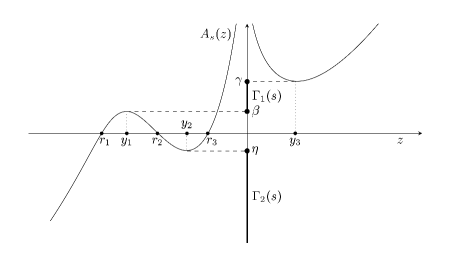
The symbol (2.14) with the functions $b(s)$, $c(s)$ and $d(s)$ from (2.13) allows for a factorization

As​(z)=(z+s​(s+p))​(z+s​(s+p+q))​(z+(s+p)​(s+p+q))z2.subscriptπ΄π‘ π‘§π‘§π‘ π‘ π‘π‘§π‘ π‘ π‘π‘žπ‘§π‘ π‘π‘ π‘π‘žsuperscript𝑧2\displaystyle A_{s}(z)=\frac{(z+s(s+p))(z+s(s+p+q))(z+(s+p)(s+p+q))}{z^{2}}. (3.1)

By (3.1), it follows that $A_{s}$ has three negative simple zeros $r_{1},r_{2},r_{3}$. We order them so that

$$r_{1}<r_{2}<r_{3}<0;$$

see Figure 4 for the graph of $A_{s}(z)$.

The derivative of $A_{s}(z)$,

$$A^{\prime}_{s}(z)=1-c(s)z^{-2}-2d(s)z^{-3},$$

has three roots in the complex plane. From FigureΒ 4, we see that all zeros of $A_{s}^{\prime}$ are real. We denote the zeros of $A^{\prime}(z)$ by $y_{1}$, $y_{2}$ and $y_{3}$ so that

$$y_{1}<y_{2}<0<y_{3},$$ (3.2)

as indicated in Figure 4. To emphasize the dependence on $s$, we also write $y_{1}(s)$, $y_{2}(s)$ and $y_{3}(s)$.

Refer to caption
Figure 4: The graph of $A_{s}(z)$ (1.6), $z\in\mathbb{R}$.

Before proving Proposition 2.3 we first need two lemmas. The fact that all the zeros $r_{j}$ of the symbol $A_{s}$ are strictly negative plays a key role in these proofs.

Lemma 3.1.

Assume that $z_{1},z_{2}\in\mathbb{C}$ are such that z1β‰ z2subscript𝑧1subscript𝑧2z_{1}\neq z_{2}, $|z_{1}|=|z_{2}|$ and $A_{s}(z_{1})=A_{s}(z_{2})=x$. Then $z_{1}=\bar{z}_{2}$ and $x\in\mathbb{R}$.

Proof.

This lemma is essentially Lemma 4.1 in [14]. For the convenience of the readers, we repeat the proof here.

Since z1β‰ z2subscript𝑧1subscript𝑧2z_{1}\neq z_{2} and $|z_{1}|=|z_{2}|$, we may assume $z_{1}=\rho e^{i\theta_{1}}$, $z_{2}=\rho e^{i\theta_{2}}$ with $\rho>0$ and ΞΈ1β‰ ΞΈ2subscriptπœƒ1subscriptπœƒ2\theta_{1}\neq\theta_{2}, $\theta_{1,2}\in[-\pi,\pi]$. Since the zeros $r_{j}$ of $A_{s}$ are strictly negative, it is easily seen that f​(ΞΈ):=|As​(ρ​ei​θ)|assignπ‘“πœƒsubscriptπ΄π‘ πœŒsuperscriptπ‘’π‘–πœƒf(\theta):=|A_{s}(\rho e^{i\theta})| is an even function on $[-\pi,\pi]$, which is strictly decreasing as $\theta$ increases from 00 to $\pi$. Hence, the equality

|As​(ρ​ei​θ1)|=|As​(ρ​ei​θ2)|subscriptπ΄π‘ πœŒsuperscript𝑒𝑖subscriptπœƒ1subscriptπ΄π‘ πœŒsuperscript𝑒𝑖subscriptπœƒ2|A_{s}(\rho e^{i\theta_{1}})|=|A_{s}(\rho e^{i\theta_{2}})|

holds if and only if $\theta_{2}=-\theta_{1}$. It then follows that $z_{1}=\bar{z}_{2}$, and

$$x=A_{s}(z_{1})=\overline{A_{s}(\bar{z}_{1})}=\overline{A_{s}(z_{2})}=\overline{x},$$

so that $x\in\mathbb{R}$. ∎

Lemma 3.2.

For each $s>0$, we have $\Gamma_{1}(s)\cup\Gamma_{2}(s)\subset\mathbb{R}$ and $\Gamma_{1}(s)\cap\Gamma_{2}(s)=\emptyset$.

Proof.

To show $\Gamma_{1}(s)\cup\Gamma_{2}(s)\subset\mathbb{R}$, we consider two cases, based on whether the equation $A_{s}(z)-x=0$ has a double root or not. If $x\in\Gamma_{1}(s)\cup\Gamma_{2}(s)$ and $A_{s}(z)-x=0$ has a double root, then there exists $z_{1}\in\mathbb{C}$ such that $A_{s}(z_{1})=x$ and $A^{\prime}_{s}(z_{1})=0$. Since all zeros of $A^{\prime}_{s}(z)$ are real, it follows that $x\in\mathbb{R}$. On the other hand, suppose $x\in\Gamma_{1}(s)\cup\Gamma_{2}(s)$ and $A_{s}(z)-x=0$ does not have a double root, then there exist $z_{1},z_{2}\in\mathbb{C}$ such that z1β‰ z2subscript𝑧1subscript𝑧2z_{1}\neq z_{2}, $|z_{1}|=|z_{2}|$ and $x=A_{s}(z_{1})=A_{s}(z_{2})$. We then conclude form LemmaΒ 3.1 that $x\in\mathbb{R}$. This proves that $\Gamma_{1}(s)\cup\Gamma_{2}(s)\subset\mathbb{R}$.

To show $\Gamma_{1}(s)\cap\Gamma_{2}(s)=\emptyset$, we observe that, if $x\in\Gamma_{1}(s)\cap\Gamma_{2}(s)$, there exist three solutions of $A_{s}(z)=x$, one negative solution $z_{1}<0$ and two complex conjugated solutions $z_{2}$ and $\bar{z}_{2}$ . Moreover z1β‰ z2subscript𝑧1subscript𝑧2z_{1}\neq z_{2} and z1β‰ zΒ―2subscript𝑧1subscript¯𝑧2z_{1}\neq\bar{z}_{2}. Now $|z_{1}|=|z_{2}|$ ($x\in\Gamma_{1}(s)$) and $A_{s}(z_{1})=A_{s}(z_{2})$. Again, by Lemma 3.1, we obtain $z_{1}=\bar{z}_{2}$, which is a contradiction. Therefore, $\Gamma_{1}(s)\cap\Gamma_{2}(s)=\emptyset$. ∎

Proof of Proposition 2.3.

Since $p$ and $q$ are positive, there are three local extrema of $A_{s}(z)$, namely β​(s),γ​(s),η​(s)π›½π‘ π›Ύπ‘ πœ‚π‘ \beta(s),\gamma(s),\eta(s), such that

η​(s)<0<β​(s)<γ​(s).πœ‚π‘ 0𝛽𝑠𝛾𝑠\eta(s)<0<\beta(s)<\gamma(s).

If x∈(η​(s),β​(s))βˆͺ(γ​(s),∞)π‘₯πœ‚π‘ π›½π‘ π›Ύπ‘ x\in(\eta(s),\beta(s))\cup(\gamma(s),\infty), there exist three different real solutions of $A_{s}(z)=x$. These solutions differ in absolute value, which is obvious if x∈(η​(s),β​(s))π‘₯πœ‚π‘ π›½π‘ x\in(\eta(s),\beta(s)) (cf. Figure 4) and a consequence of Lemma 3.1 if $x\in(\gamma(s),\infty)$. On the other hand, there is one real and two complex conjugated solutions whenever x∈(βˆ’βˆž,η​(s)]βˆͺ[β​(s),γ​(s)]π‘₯πœ‚π‘ π›½π‘ π›Ύπ‘ x\in(-\infty,\eta(s)]\cup[\beta(s),\gamma(s)]. Therefore

Ξ“1​(s)βˆͺΞ“2​(s)βŠ‚(βˆ’βˆž,η​(s)]βˆͺ[β​(s),γ​(s)].subscriptΞ“1𝑠subscriptΞ“2π‘ πœ‚π‘ π›½π‘ π›Ύπ‘ \Gamma_{1}(s)\cup\Gamma_{2}(s)\subset(-\infty,\eta(s)]\cup[\beta(s),\gamma(s)].

Note that $A_{s}(z)=\gamma(s)$ has a double root at $y_{3}=y_{3}(s)>0$ and one negative root whose absolute value is less than $y_{3}(s)$. Thus $\gamma(s)\in\Gamma_{1}(s)$. By the same argument, we see $\beta(s)\in\Gamma_{1}(s)$. In view of the fact that $\Gamma_{1}(s)$ is connected (see [21],[3, Theorem 11.19]), it then follows that $\Gamma_{1}(s)=[\beta(s),\gamma(s)]$. Similarly, we notice that As​(z)=η​(s)subscriptπ΄π‘ π‘§πœ‚π‘ A_{s}(z)=\eta(s) has a double root at $y_{2}(s)<0$ and a negative root whose absolute value is larger than $|y_{2}(s)|$. Therefore $\eta_{2}(s)\in\Gamma_{2}(s)$ and Ξ“2​(s)=(βˆ’βˆž,η​(s)]subscriptΞ“2π‘ πœ‚π‘ \Gamma_{2}(s)=(-\infty,\eta(s)].

To show that $\gamma(s)$ is an increasing function, we introduce

B​(z,s)=As​(s​(s+p)​(s+p+q)zβˆ’s)=z​(z+p)​(z+p+q)zβˆ’s.𝐡𝑧𝑠subscriptπ΄π‘ π‘ π‘ π‘π‘ π‘π‘žπ‘§π‘ π‘§π‘§π‘π‘§π‘π‘žπ‘§π‘ B(z,s)=A_{s}\Big{(}\frac{s(s+p)(s+p+q)}{z-s}\Big{)}=\frac{z(z+p)(z+p+q)}{z-s}. (3.3)

Taking the partial derivative of $B(z,s)$ with respect to $s$, we obtain

βˆ‚B​(z,s)βˆ‚s=z​(z+p)​(z+p+q)(zβˆ’s)2.π΅π‘§π‘ π‘ π‘§π‘§π‘π‘§π‘π‘žsuperscript𝑧𝑠2\frac{\partial B(z,s)}{\partial s}=\frac{z(z+p)(z+p+q)}{(z-s)^{2}}. (3.4)

As a function of $z$, it is easily seen that $B(z,s)$ has a local minimum at s+s​(s+p)​(s+p+q)/y3​(s)π‘ π‘ π‘ π‘π‘ π‘π‘žsubscript𝑦3𝑠s+s(s+p)(s+p+q)/y_{3}(s) and

γ​(s)=As​(y3​(s))=B​(s+s​(s+p)​(s+p+q)/y3​(s),s).𝛾𝑠subscript𝐴𝑠subscript𝑦3π‘ π΅π‘ π‘ π‘ π‘π‘ π‘π‘žsubscript𝑦3𝑠𝑠\gamma(s)=A_{s}(y_{3}(s))=B(s+s(s+p)(s+p+q)/y_{3}(s),s).

This, together with (3.4), implies that

$\displaystyle\gamma^{\prime}(s)$ =βˆ‚B​(s+s​(s+p)​(s+p+q)/y3​(s),s)βˆ‚zβ€‹βˆ‚(s+s​(s+p)​(s+p+q)/y3​(s))βˆ‚sabsentπ΅π‘ π‘ π‘ π‘π‘ π‘π‘žsubscript𝑦3π‘ π‘ π‘§π‘ π‘ π‘ π‘π‘ π‘π‘žsubscript𝑦3𝑠𝑠\displaystyle=\frac{\partial B(s+s(s+p)(s+p+q)/y_{3}(s),s)}{\partial z}\frac{\partial(s+s(s+p)(s+p+q)/y_{3}(s))}{\partial s}
+βˆ‚B​(s+s​(s+p)​(s+p+q)/y3​(s),s)βˆ‚sπ΅π‘ π‘ π‘ π‘π‘ π‘π‘žsubscript𝑦3𝑠𝑠𝑠\displaystyle~{}~{}~{}~{}~{}+\frac{\partial B(s+s(s+p)(s+p+q)/y_{3}(s),s)}{\partial s}
=βˆ‚B​(s+s​(s+p)​(s+p+q)/y3​(s),s)βˆ‚sabsentπ΅π‘ π‘ π‘ π‘π‘ π‘π‘žsubscript𝑦3𝑠𝑠𝑠\displaystyle=\frac{\partial B(s+s(s+p)(s+p+q)/y_{3}(s),s)}{\partial s}
=z^3​(s)​(z^3​(s)+p)​(z^3​(s)+p+q)(z^3​(s)βˆ’s)2,absentsubscript^𝑧3𝑠subscript^𝑧3𝑠𝑝subscript^𝑧3π‘ π‘π‘žsuperscriptsubscript^𝑧3𝑠𝑠2\displaystyle=\frac{\hat{z}_{3}(s)(\hat{z}_{3}(s)+p)(\hat{z}_{3}(s)+p+q)}{(\hat{z}_{3}(s)-s)^{2}}, (3.5)

where z^3​(s)=s+s​(s+p)​(s+p+q)/y3​(s)subscript^𝑧3π‘ π‘ π‘ π‘ π‘π‘ π‘π‘žsubscript𝑦3𝑠\hat{z}_{3}(s)=s+s(s+p)(s+p+q)/y_{3}(s). As $y_{3}(s)>0$ and $p,q>0$, we have $\hat{z}_{3}(s)>0$ for all $s>0$. Therefore $\gamma(s)$ is increasing on $(0,\infty)$ by (3). The monotonicity of $\beta(s)$ and η​(s)πœ‚π‘ \eta(s) can be proved in similar manners. Indeed, by the same argument, we have

η′​(s)superscriptπœ‚β€²π‘ \displaystyle\eta^{\prime}(s) =z^2​(s)​(z^2​(s)+p)​(z^2​(s)+p+q)(z^2​(s)βˆ’s)2,absentsubscript^𝑧2𝑠subscript^𝑧2𝑠𝑝subscript^𝑧2π‘ π‘π‘žsuperscriptsubscript^𝑧2𝑠𝑠2\displaystyle=\frac{\hat{z}_{2}(s)(\hat{z}_{2}(s)+p)(\hat{z}_{2}(s)+p+q)}{(\hat{z}_{2}(s)-s)^{2}}, (3.6)
$\displaystyle\beta^{\prime}(s)$ =z^1​(s)​(z^1​(s)+p)​(z^1​(s)+p+q)(z^1​(s)βˆ’s)2,absentsubscript^𝑧1𝑠subscript^𝑧1𝑠𝑝subscript^𝑧1π‘ π‘π‘žsuperscriptsubscript^𝑧1𝑠𝑠2\displaystyle=\frac{\hat{z}_{1}(s)(\hat{z}_{1}(s)+p)(\hat{z}_{1}(s)+p+q)}{(\hat{z}_{1}(s)-s)^{2}}, (3.7)

where z^j​(s)=s+s​(s+p)​(s+p+q)/yj​(s)subscript^π‘§π‘—π‘ π‘ π‘ π‘ π‘π‘ π‘π‘žsubscript𝑦𝑗𝑠\hat{z}_{j}(s)=s+s(s+p)(s+p+q)/y_{j}(s), $j=1,2$. Note that $y_{2}(s)$ and $y_{1}(s)$ are local extreme points of $A_{s}(z)$, whose zeros are $-s(s+p)$, βˆ’s​(s+p+q)π‘ π‘ π‘π‘ž-s(s+p+q) and βˆ’(s+p)​(s+p+q)π‘ π‘π‘ π‘π‘ž-(s+p)(s+p+q). Therefore, in view of (3.2) (see also Figure 4), we have

βˆ’s​(s+p+q)<y2​(s)<βˆ’s​(s+p)​andβˆ’(s+p)​(s+p+q)<y1​(s)<βˆ’s​(s+p+q),π‘ π‘ π‘π‘žsubscript𝑦2𝑠𝑠𝑠𝑝andπ‘ π‘π‘ π‘π‘žsubscript𝑦1π‘ π‘ π‘ π‘π‘ž-s(s+p+q)<y_{2}(s)<-s(s+p)~{}~{}\textrm{and}~{}~{}-(s+p)(s+p+q)<y_{1}(s)<-s(s+p+q),

which implies

$$-(p+q)<\hat{z}_{2}(s)<-p~{}~{}\textrm{and}~{}~{}-p<\hat{z}_{1}(s)<0.$$ (3.8)

Combining (3.6)–(3.8), it follows that η′​(s)>0superscriptπœ‚β€²π‘ 0\eta^{\prime}(s)>0 and $\beta^{\prime}(s)<0$ for all $s>0$, which gives the desired monotonicity of $\beta(s)$ and η​(s)πœ‚π‘ \eta(s).

Finally, we come to the boundary values of $\gamma(s)$, $\beta(s)$ and η​(s)πœ‚π‘ \eta(s). A straightforward calculation yields that $y_{1}(s)$, $y_{2}(s)$ and $y_{3}(s)$ have the following behavior as $s\rightarrow 0$

$\displaystyle y_{1}(s)$ =βˆ’p​(p+q)​(2​p+q)​s+π’ͺ​(s),absentπ‘π‘π‘ž2π‘π‘žπ‘ π’ͺ𝑠\displaystyle=-\sqrt{p(p+q)(2p+q)s}+\mathcal{O}(s),
$\displaystyle y_{2}(s)$ =βˆ’2​p​(p+q)2​p+q​s+π’ͺ​(s2),absent2π‘π‘π‘ž2π‘π‘žπ‘ π’ͺsuperscript𝑠2\displaystyle=-\frac{2p(p+q)}{2p+q}s+\mathcal{O}(s^{2}),
$\displaystyle y_{3}(s)$ =p​(p+q)​(2​p+q)​s+π’ͺ​(s).absentπ‘π‘π‘ž2π‘π‘žπ‘ π’ͺ𝑠\displaystyle=\sqrt{p(p+q)(2p+q)s}+\mathcal{O}(s).

Hence,

$\displaystyle\gamma(s)=A_{s}(y_{3}(s))$ $\displaystyle=p(p+q)+\mathcal{O}(s),$
η​(s)=As​(y2​(s))πœ‚π‘ subscript𝐴𝑠subscript𝑦2𝑠\displaystyle\eta(s)=A_{s}(y_{2}(s)) $\displaystyle=-\frac{1}{4}q^{2}+\mathcal{O}(s),$
$\displaystyle\beta(s)=A_{s}(y_{1}(s))$ $\displaystyle=p(p+q)+\mathcal{O}(s),$

as $s\to 0+$. This proves the limits

limsβ†’0+β​(s)=limsβ†’0+γ​(s)=p​(p+q)​and​limsβ†’0+η​(s)=βˆ’14​q2.subscript→𝑠limit-from0𝛽𝑠subscript→𝑠limit-from0π›Ύπ‘ π‘π‘π‘žandsubscript→𝑠limit-from0πœ‚π‘ 14superscriptπ‘ž2\lim_{s\rightarrow 0+}\beta(s)=\lim_{s\rightarrow 0+}\gamma(s)=p(p+q)~{}~{}\textrm{and}~{}~{}\lim_{s\rightarrow 0+}\eta(s)=-\frac{1}{4}q^{2}.

On the other hand, note that $y_{1}(s)$, $y_{2}(s)$ and $y_{3}(s)$ have the following behavior as sβ†’βˆžβ†’π‘ s\rightarrow\infty,

$\displaystyle y_{1}(s)$ $\displaystyle=-s^{2}+c_{1}s+\mathcal{O}(1),$
$\displaystyle y_{2}(s)$ $\displaystyle=-s^{2}+c_{2}s+\mathcal{O}(1),$
$\displaystyle y_{3}(s)$ $\displaystyle=2s^{2}+\frac{8p-4q}{3}s+\mathcal{O}(1),$

where $c_{1}=(-4p-2q-\sqrt{p^{2}+pq+q^{2}})/3$ and $c_{2}=(-4p-2q+\sqrt{p^{2}+pq+q^{2}})/3$, the limits of $\gamma(s)$, $\beta(s)$ and η​(s)πœ‚π‘ \eta(s) as sβ†’βˆžβ†’π‘ s\to\infty can be obtained in a manner similar to the situation $s\to 0+$, we omit the details and this completes the proof of the Proposition 2.3. ∎

4 Proof of TheoremΒ 2.4

From the definitions of $\nu_{1}^{\xi}$ and $\nu_{2}^{\xi}$ in (2.16) and (2.18), it is clear that $\mathrm{supp}(\nu_{1}^{\xi})\subset[0,\infty)$, $\int d\nu_{1}^{\xi}=1$ and $\mathrm{supp}(\nu_{2}^{\xi})\subset(-\infty,0]$, $\int d\nu_{2}^{\xi}=1/2$. Indeed, on account of the fact that the sets $\Gamma_{1}(s)=\mathrm{supp}(\mu_{1}^{s})$ and $\Gamma_{2}(s)=\mathrm{supp}(\mu_{2}^{s})$ are increasing as $s$ increases (see Proposition 2.3), it follows that

supp​(Ξ½1ΞΎ)=⋃s≀ξΓ1​(s)=Ξ“1​(ΞΎ)suppsuperscriptsubscript𝜈1πœ‰subscriptπ‘ πœ‰subscriptΞ“1𝑠subscriptΞ“1πœ‰\mathrm{supp}(\nu_{1}^{\xi})=\bigcup_{s\leq\xi}\Gamma_{1}(s)=\Gamma_{1}(\xi) (4.1)

and

supp​(Ξ½2ΞΎ)=⋃s≀ξΓ2​(s)=Ξ“2​(ΞΎ).suppsuperscriptsubscript𝜈2πœ‰subscriptπ‘ πœ‰subscriptΞ“2𝑠subscriptΞ“2πœ‰\mathrm{supp}(\nu_{2}^{\xi})=\bigcup_{s\leq\xi}\Gamma_{2}(s)=\Gamma_{2}(\xi). (4.2)

Thus, in order to show that $(\nu_{1}^{\xi},\nu_{2}^{\xi})$ is the minimizer of the energy functional (2.4) under the conditions stated in TheoremΒ 2.4, it suffices to prove that the vector $(\nu_{1}^{\xi},\nu_{2}^{\xi})$ satisfies the variational conditions (2.25) and (2.26).

The basic idea is, as mentioned in Subsection 2.2, to integrate the variational conditions (2.20) and (2.21) with respect to $s$ from 00 to $\xi$. Here, we need a more general expression for the variational conditions (2.20) and (2.21), namely

2β€‹βˆ«log⁑|xβˆ’y|​d​μ1s​(y)βˆ’βˆ«log⁑|xβˆ’y|​d​μ2s​(y)βˆ’β„“s2π‘₯𝑦𝑑subscriptsuperscriptπœ‡π‘ 1𝑦π‘₯𝑦𝑑subscriptsuperscriptπœ‡π‘ 2𝑦superscriptℓ𝑠\displaystyle 2\int\log|x-y|d\mu^{s}_{1}(y)-\int\log|x-y|d\mu^{s}_{2}(y)-\ell^{s} $\displaystyle=\log\left|\frac{z_{1}(x,s)}{z_{2}(x,s)}\right|,$ (4.3)
2β€‹βˆ«log⁑|xβˆ’y|​d​μ2s​(y)βˆ’βˆ«log⁑|xβˆ’y|​d​μ1s​(y)2π‘₯𝑦𝑑subscriptsuperscriptπœ‡π‘ 2𝑦π‘₯𝑦𝑑subscriptsuperscriptπœ‡π‘ 1𝑦\displaystyle 2\int\log|x-y|d\mu^{s}_{2}(y)-\int\log|x-y|d\mu^{s}_{1}(y) $\displaystyle=\log\left|\frac{z_{2}(x,s)}{z_{3}(x,s)}\right|,$ (4.4)

for all $x\in\mathbb{C}$, which are contained in the proof of Theorem 2.3 of [10]. These conditions reduce to (2.20) and (2.21) whenever $x\in\Gamma_{1}(s)$ and $x\in\Gamma_{2}(s)$, respectively.

Proofs of (2.25) and (2.26).

Multiplying both sides of (4.3) by $1/\xi$ and integrating with respect to $s$ from 00 to $\xi$, we obtain from interchanging the order of integration that

$$2\int\log|x-y|d\nu^{\xi}_{1}(y)-\int\log|x-y|d\nu^{\xi}_{2}(y)-\ell=\frac{1}{\xi}\int_{0}^{\xi}\log\left|\frac{z_{1}(x,s)}{z_{2}(x,s)}\right|ds,$$ (4.5)

for all $x\in\mathbb{C}$ and some constant $\ell\in\mathbb{R}$. The measures $\nu_{1}^{\xi}$ and $\nu_{2}^{\xi}$ in (4.5) are defined in (2.16) and (2.18), respectively.

Let $x\geq 0$. Since $|z_{1}(x,s)|\geq|z_{2}(x,s)|$ for every $s$, it follows from (4.5) and (2.24) that

$$2\int\log|x-y|d\nu^{\xi}_{1}(y)-\int\log|x-y|d\nu^{\xi}_{2}(y)-\ell\leq\frac{1}{\xi}\int_{0}^{\infty}\log\left|\frac{z_{1}(x,s)}{z_{2}(x,s)}\right|ds=\frac{1}{\xi}V_{1}(x).$$ (4.6)

Suppose now $x\in\mathrm{supp}(\nu_{1}^{\xi})$, then $x\in\Gamma_{1}(\xi)$ by (4.1), and therefore $x\in\Gamma_{1}(s)$ for every sβ‰₯ΞΎπ‘ πœ‰s\geq\xi, since the sets are increasing. Thus $|z_{1}(x,s)|=|z_{2}(x,s)|$ for every sβ‰₯ΞΎπ‘ πœ‰s\geq\xi, and equality holds in (4.6) for $x\in\mathrm{supp}(\nu_{1}^{\xi})$. This completes the proof of (2.25).

The variational condition (2.26) for $\nu_{2}^{\xi}$ can be proved in a manner similar to (2.25) by using (4.4) and (4.2), we omit the details. ∎

5 Proof of TheoremΒ 2.5

We conclude this paper with the proof of TheoremΒ 2.5. We start with the following lemma that embodies the behavior of three solutions of $A_{s}(z)$ as $s\to 0+$.

Lemma 5.1.

Let $A_{s}(z)$ be given by (3.1), and let $z_{1}(x,s)$, $z_{2}(x,s)$ and $z_{3}(x,s)$ be the solutions of $A_{s}(z)=x$, ordered as in (1.8). Then

$\displaystyle\lim_{s\to 0+}z_{1}(x,s)$ $\displaystyle=x-p(p+q),$ (5.1)
$\displaystyle\lim_{s\to 0+}s^{-1}z_{2}(x,s)$ $\displaystyle=-\frac{p(p+q)(2p+q+\sqrt{q^{2}+4x})}{2(p^{2}+pq-x)},$
$\displaystyle\lim_{s\to 0+}s^{-1}z_{3}(x,s)$ $\displaystyle=-\frac{p(p+q)(2p+q-\sqrt{q^{2}+4x})}{2(p^{2}+pq-x)}.$
Proof.

The lemma follows by a straightforward computation. ∎

To prove TheoremΒ 2.5, we need to establish the identities (2.27)–(2.30).

Proof of (2.27).

Let $x>0$. From Proposition 2.3, it follows that there exists a unique $s^{*}(x)\geq 0$ so that for all $s>0$,

xβˆˆΞ“1​(s)⟺sβ‰₯sβˆ—β€‹(x).formulae-sequenceπ‘₯subscriptΞ“1π‘ βŸΊπ‘ superscript𝑠π‘₯x\in\Gamma_{1}(s)\quad\Longleftrightarrow\quad s\geq s^{*}(x). (5.2)

Then $\log|z_{1}(x,s)/z_{2}(x,s)|=0$ for all $s\geq s^{*}(x)$, and so by (2.24)

$$V_{1}(x)=\int_{0}^{s^{*}(x)}\log\left|\frac{z_{1}(x,s)}{z_{2}(x,s)}\right|ds.$$ (5.3)

There is a special value

$$x_{0}=p(p+q)=\lim_{s\to 0+}\beta(s)=\lim_{s\to 0+}\gamma(s)$$

that belongs to every $\Gamma_{1}(s)$ for any $s>0$. Then $s^{*}(x_{0})=0$ and

$$V_{1}(x_{0})=0.$$ (5.4)

The derivative of (5.3) is

$$V_{1}^{\prime}(x)=\int_{0}^{s^{*}(x)}\left(\frac{1}{z_{1}(x,s)}\frac{\partial z_{1}(x,s)}{\partial x}-\frac{1}{z_{2}(x,s)}\frac{\partial z_{2}(x,s)}{\partial x}\right)ds.$$ (5.5)

In order to evaluate this integral, we introduce new variables

z~j​(x,s)=s​(s+p)​(s+p+q)zj​(x,s)+s,j=1,2,3.formulae-sequencesubscript~𝑧𝑗π‘₯π‘ π‘ π‘ π‘π‘ π‘π‘žsubscript𝑧𝑗π‘₯𝑠𝑠𝑗123\widetilde{z}_{j}(x,s)=\frac{s(s+p)(s+p+q)}{z_{j}(x,s)}+s,\qquad j=1,2,3. (5.6)

Since each $z_{j}(x,s)$ is a solution of $A_{s}(z)=x$, it follows that $\widetilde{z}_{j}(x,s)$ for $j=1,2,3$ is a solution of the equation $B(z,s)=x$, where

B​(z,s)=z​(z+p)​(z+p+q)zβˆ’s;π΅π‘§π‘ π‘§π‘§π‘π‘§π‘π‘žπ‘§π‘ B(z,s)=\frac{z(z+p)(z+p+q)}{z-s}; (5.7)

see (3.3).

Taking partial derivatives with respect to $s$ and $x$ on both sides of $B(\widetilde{z}_{j}(x,s),s)=x$, and applying the chain rule, we obtain

$\displaystyle\left(\frac{\partial B}{\partial z}(\widetilde{z}_{j}(x,s),s)\right)\,\frac{\partial\widetilde{z}_{j}(x,s)}{\partial s}+\frac{\partial B}{\partial s}(\widetilde{z}_{j}(x,s),s)$ $\displaystyle=0,$ (5.8)
$\displaystyle\left(\frac{\partial B}{\partial z}(\widetilde{z}_{j}(x,s),s)\right)\frac{\partial\widetilde{z}_{j}(x,s)}{\partial x}$ $\displaystyle=1$

for $j=1,2,3$. From (5.7), it is elementary to deduce that

βˆ‚Bβˆ‚s​(z~j​(x,s),s)=z~j​(x,s)​(z~j​(x,s)+p)​(z~j​(x,s)+p+q)(z~j​(x,s)βˆ’s)2=xz~j​(x,s)βˆ’s.𝐡𝑠subscript~𝑧𝑗π‘₯𝑠𝑠subscript~𝑧𝑗π‘₯𝑠subscript~𝑧𝑗π‘₯𝑠𝑝subscript~𝑧𝑗π‘₯π‘ π‘π‘žsuperscriptsubscript~𝑧𝑗π‘₯𝑠𝑠2π‘₯subscript~𝑧𝑗π‘₯𝑠𝑠\frac{\partial B}{\partial s}(\widetilde{z}_{j}(x,s),s)=\frac{\widetilde{z}_{j}(x,s)(\widetilde{z}_{j}(x,s)+p)(\widetilde{z}_{j}(x,s)+p+q)}{(\widetilde{z}_{j}(x,s)-s)^{2}}=\frac{x}{\widetilde{z}_{j}(x,s)-s}.

Combining this with (5.8), we obtain

$$\frac{x}{\widetilde{z}_{j}(x,s)-s}\frac{\partial\widetilde{z}_{j}(x,s)}{\partial x}=-\frac{\partial\widetilde{z}_{j}(x,s)}{\partial s},\qquad j=1,2,3.$$ (5.9)

By (5.6), we also note that

βˆ‚z~j​(x,s)βˆ‚x=βˆ’s​(s+p)​(s+p+q)zj2​(x,s)β€‹βˆ‚zj​(x,s)βˆ‚x=βˆ’z~j​(x,s)βˆ’szj​(x,s)β€‹βˆ‚zj​(x,s)βˆ‚s.subscript~𝑧𝑗π‘₯𝑠π‘₯π‘ π‘ π‘π‘ π‘π‘žsuperscriptsubscript𝑧𝑗2π‘₯𝑠subscript𝑧𝑗π‘₯𝑠π‘₯subscript~𝑧𝑗π‘₯𝑠𝑠subscript𝑧𝑗π‘₯𝑠subscript𝑧𝑗π‘₯𝑠𝑠\frac{\partial\widetilde{z}_{j}(x,s)}{\partial x}=-\frac{s(s+p)(s+p+q)}{z_{j}^{2}(x,s)}\frac{\partial z_{j}(x,s)}{\partial x}=-\frac{\widetilde{z}_{j}(x,s)-s}{z_{j}(x,s)}\frac{\partial z_{j}(x,s)}{\partial s}. (5.10)

Substituting (5.10) into (5.9) gives

$$\frac{1}{z_{j}(x,s)}\frac{\partial z_{j}(x,s)}{\partial s}=\frac{1}{x}\frac{\partial\widetilde{z}_{j}(x,s)}{\partial s},\qquad j=1,2,3.$$ (5.11)

Hence, using (5.11) in (5.5) we get

$$V_{1}^{\prime}(x)=\frac{1}{x}\int_{0}^{s^{*}(x)}\left(\frac{\partial\widetilde{z}_{1}(x,s)}{\partial s}-\frac{\partial\widetilde{z}_{2}(x,s)}{\partial s}\right)ds.$$

It then follows from the fundamental theorem of calculus that

$$V_{1}^{\prime}(x)=\frac{1}{x}[\widetilde{z}_{1}(x,s^{*}(x))-\widetilde{z}_{2}(x,s^{*}(x))-\lim_{s\to 0+}(\widetilde{z}_{1}(x,s)-\widetilde{z}_{2}(x,s))].$$ (5.12)

By definition, $s^{*}(x)$ is the smallest value of $s\geq 0$ for which $x\in\Gamma_{1}(s)$. Then $x=\gamma(s^{*}(x))$ if $x_{0}<x$ and $x=\beta(s^{*}(x))$ if $0<x<x_{0}$. We can observe from Figure 4 that $z_{1}(\gamma(s),s)=z_{2}(\gamma(s),s)$ and $z_{1}(\beta(s),s)=z_{2}(\beta(s),s)$. Therefore,

$$\widetilde{z}_{1}(x,s^{*}(x))=\widetilde{z}_{2}(x,s^{*}(x))$$

and (5.12) reduces to

$$V_{1}^{\prime}(x)=-\frac{1}{x}\lim_{s\to 0+}(\widetilde{z}_{1}(x,s)-\widetilde{z}_{2}(x,s)).$$ (5.13)

From (5.6) and LemmaΒ 5.1, we find that

$\displaystyle\lim_{s\rightarrow 0+}\widetilde{z}_{1}(x,s)=0\qquad\text{and}\qquad\lim_{s\rightarrow 0+}\widetilde{z}_{2}(x,s)=-\frac{2(p^{2}+pq-x)}{2p+q+\sqrt{q^{2}+4x}}.$

Then (5.13) leads to

$$V_{1}^{\prime}(x)=-\frac{1}{x}\frac{2(p^{2}+pq-x)}{2p+q+\sqrt{q^{2}+4x}}.$$ (5.14)

We obtain $V_{1}(x)$ by integrating (5.14) with respect to $x$, which gives

$$V_{1}(x)=\sqrt{q^{2}+4x}-p\log(4x)-q\log(\sqrt{q^{2}+4x}+q)+C.$$

The constant of integration $C$ can be determined by requiring $V_{1}(x_{0})=0$; see (5.4). This gives

$$C=-2p-q+p\log(4p^{2}+4pq)+q\log(2p+2q),$$

and (2.27) is proved. ∎

Proof of (2.28).

Let $x<0$. Again, it follows from Proposition 2.3 that there exists a unique $s^{*}(x)\geq 0$ so that for all $s>0$,

xβˆˆΞ“2​(s)⟺sβ‰₯sβˆ—β€‹(x).formulae-sequenceπ‘₯subscriptΞ“2π‘ βŸΊπ‘ superscript𝑠π‘₯x\in\Gamma_{2}(s)\quad\Longleftrightarrow\quad s\geq s^{*}(x). (5.15)

Then $\log|z_{2}(x,s)/z_{3}(x,s)|=0$ for all $s\geq s^{*}(x)$, and so by (2.24)

$$V_{2}(x)=\int_{0}^{s^{*}(x)}\log\left|\frac{z_{2}(x,s)}{z_{3}(x,s)}\right|ds.$$ (5.16)

There also exists a special value

x~0=βˆ’q2/4=limsβ†’0+η​(s)subscript~π‘₯0superscriptπ‘ž24subscript→𝑠limit-from0πœ‚π‘ \widetilde{x}_{0}=-q^{2}/4=\lim_{s\to 0+}\eta(s)

so that $x\in\Gamma_{2}(s)$ for any $s>0$ if $x\leq\widetilde{x}_{0}$. Then, for any $x\leq\widetilde{x}_{0}$, we have $s^{*}(x)=0$ and

$$V_{2}(x)=0.$$ (5.17)

If $-q^{2}/4=\widetilde{x}_{0}\leq x<0$, by the same argument in the proof of (2.27), we have

$$V_{2}^{\prime}(x)=-\frac{1}{x}\lim_{s\to 0+}(\widetilde{z}_{2}(x,s)-\widetilde{z}_{3}(x,s)),$$ (5.18)

where $\widetilde{z}_{j}(x,s)$, $j=2,3$ are given in (5.6). From LemmaΒ 5.1, we see

$\displaystyle\lim_{s\rightarrow 0+}\widetilde{z}_{2}(x,s)=-\frac{2(p^{2}+pq-x)}{2p+q+\sqrt{q^{2}+4x}}\qquad\text{and}\qquad\lim_{s\rightarrow 0+}\widetilde{z}_{3}(x,s)=-\frac{2(p^{2}+pq-x)}{2p+q-\sqrt{q^{2}+4x}}.$

Hence, (5.18) leads to

$$V_{2}^{\prime}(x)=-\frac{\sqrt{q^{2}+4x}}{x}.$$ (5.19)

By integrating (5.19) with respect to $x$, we obtain

$$V_{2}(x)=-2\sqrt{q^{2}+4x}+q\log\Big{(}\frac{q+\sqrt{q^{2}+4x}}{q-\sqrt{q^{2}+4x}}\Big{)}+\widetilde{C},$$

for $-q^{2}/4\leq x<0$. The constant of integration $\widetilde{C}$ can be determined by requiring $V_{2}(\widetilde{x}_{0})=0$; see (5.17). This leads to $\widetilde{C}=0$ and (2.28) is proved. ∎

Proofs of (2.29) and (2.30).

By the definitions of $\nu_{1}^{\xi}$ and $\nu_{2}^{\xi}$ in (2.16) and (2.18), we obtain from (1.10) and (2.17) that

$\displaystyle\frac{d\nu_{1}^{\xi}}{dx}(x)=\frac{1}{2\pi i\xi}\int_{0}^{\xi}\left(\frac{1}{z_{1-}(x,s)}\frac{\partial z_{1-}(x,s)}{\partial x}-\frac{1}{z_{1+}(x,s)}\frac{\partial z_{1+}(x,s)}{\partial x}\right)ds,$
$\displaystyle\frac{d\nu_{2}^{\xi}}{dx}(x)=\frac{1}{2\pi i\xi}\int_{0}^{\xi}\left(\frac{1}{z_{2+}(x,s)}\frac{\partial z_{2+}(x,s)}{\partial x}-\frac{1}{z_{2-}(x,s)}\frac{\partial z_{2-}(x,s)}{\partial x}\right)ds.$

With $s^{*}(x)$ given in (5.2) and (5.15), it is readily seen that

$\displaystyle\frac{d\nu_{1}^{\xi}}{dx}(x)=\frac{1}{2\pi i\xi}\int_{s^{*}(x)}^{\xi}\left(\frac{1}{z_{1-}(x,s)}\frac{\partial z_{1-}(x,s)}{\partial x}-\frac{1}{z_{1+}(x,s)}\frac{\partial z_{1+}(x,s)}{\partial x}\right)ds,$
$\displaystyle\frac{d\nu_{2}^{\xi}}{dx}(x)=\frac{1}{2\pi i\xi}\int_{s^{*}(x)}^{\xi}\left(\frac{1}{z_{2+}(x,s)}\frac{\partial z_{2+}(x,s)}{\partial x}-\frac{1}{z_{2-}(x,s)}\frac{\partial z_{2-}(x,s)}{\partial x}\right)ds.$

Now, by introducing the change of variable (5.6), one can evaluate the above integrals using similar methods as given in the proofs of (2.27) and (2.28). We omit the details and this completes the proof of Theorem 2.5. ∎

Acknowledgements

The authors are supported by the Belgian Interuniversity Attraction Pole P06/02. The first author is supported by FWO-Flanders project G.0427.09. The second author is supported by K. U. Leuven research grant OT/08/33.

References

  • [1] A.I. Aptekarev, V. Kalyagin, G. LΓ³pez Lagomasino, and I.A. Rocha: On the limit behavior of recurrence coefficients for multiple orthogonal polynomials, J. Approx. Theory 139 (2006), 346–370.
  • [2] Y. Ben Cheikh and K. Douak: On two-orthogonal polynomials realted to the Bateman’s $J_{n}^{u,v}-$fuction, Meth. Appl. Anal. 7 (2000), 641–662.
  • [3] A. BΓΆttcher and S.M. Grudsky: Spectral properties of banded Toeplitz matrices, SIAM, Philadelphia, PA, 2005.
  • [4] E. Coussement, J. Coussement, and W. Van Assche: Asymptotic zero distribution for a class of multiple orthogonal polynomials, Trans. Amer. Math. Soc. 360 (2008), 5571–5588.
  • [5] E. Coussement and W. Van Assche: Some properties of multiple orthogonal polynomials associated with Macdonald functions, J. Comput. Appl. Math. 133 (2001), 253–261.
  • [6] E. Coussement and W. Van Assche: Multiple orthogonal polynomials associated with the modified Bessel functions of the first kind, Constr. Approx. 19 (2003), 237–263.
  • [7] E. Coussement and W. Van Assche: Asymptotics of multiple orthogonal polynomials associated with the modified Bessel functions of the first kind, J. Comput. Appl. Math. 153 (2003), 141–149.
  • [8] P. Deift, T. Kriecherbauer, K.T.-R. McLaughlin, S. Venakides, and X. Zhou: Strong asymptotics of orthogonal polynomials with respect to exponential weights, Comm. Pure Appl. Math. 52 (1999), 1491–1552.
  • [9] P. Deift, T. Kriecherbauer, K.T.-R. McLaughlin, S. Venakides, and X. Zhou: Uniform asymptotics for polynomials orthogonal with respect to varying exponential weights and applications to universality questions in random matrix theory, Comm. Pure Appl. Math. 52 (1999), 1335–1425.
  • [10] M. Duits and A.B.J. Kuijlaars: An equilibrium problem for the limiting eigenvalue distribution of banded Toeplitz matrices, SIAM J. Matrix Anal. Appl. 30 (2008), 173–196.
  • [11] M. Duits and A.B.J. Kuijlaars: Universality in the two matrix model: a Riemann-Hilbert steepest descent analysis, Comm. Pure Appl. Math. 62 (2009), 1076–1153.
  • [12] I. I. Hirschman, Jr.: The spectra of certain Toeplitz matrices, Illinois J. Math. 11 (1967), 145–159.
  • [13] A.B.J. Kuijlaars, A. MartΓ­nez Finkelstein and F. Wielonsky: Non-intersecting squared Bessel paths and multiple orthogonal polynomials for modified Bessel weights, Commun. Math. Phys. 286 (2009), 217–275.
  • [14] A.B.J. Kuijlaars and P. RomΓ‘n: Recurrence relations and vector equilibrium problems arising from a model of non-intersecting squared Bessel paths, preprint arXiv:0911.3831.
  • [15] A.B.J. Kuijlaars and W. Van Assche: The asymptotic zero distribution of orthogonal polynomials with varying recurrence coefficients, J. Approx. Theory 99 (1999), 167–197.
  • [16] P. Nevai: Orthogonal polynomials, Mem. Amer. Math. Soc. 213 (1979).
  • [17] E.M. Nikishin and V.N. Sorokin: Rational Approximants and Orthogonality, volume 92 in Translations of Mathematical Monographs. Amer. Math. Soc., Providence, RI, 1991.
  • [18] A.P. Prudnikov: Orthogonal polynomials with ultra-exponetial weight functions, in: W. Van Assche (Ed.), Open Problems, J. Comput. Appl. Math. 48 (1993), 239–241.
  • [19] E.B. Saff and V. Totik: Logarithmic Potentials with External Fields, Springer-Verlag, Berlin, 1997.
  • [20] P. Schmidt and F. Spitzer: The Toeplitz matrices of an arbitrary Laurent polynomial, Math. Scand. 8 (1960), 15–38.
  • [21] J.L. Ullman: A problem of Schmidt and Spitzer, Bull. Amer. Math. Soc. 73 (1967), 883–885.
  • [22] W. Van Assche and E. Coussement: Some classical multiple orthogonal polynomials, J. Comput. Appl. Math. 127 (2001), 317–347.
  • [23] W. Van Assche and S.B. Yakubovich: Multiple orthogonal polynomials associated with Macdonald functions, Integral Transform. Spec. Funct. 9 (2000), 229–244.