Understanding the effects of geometry and rotation on pulsar intensity profiles.

Abstract

We have developed a method to compute the possible distribution of radio emission regions in a typical pulsar magnetosphere, taking into account the viewing geometry and rotational effects of the neutron star. Our method can estimate the emission altitude and the radius of curvature of particle trajectory as a function of rotation phase for a given inclination angle, impact angle, spin-period, Lorentz factor, field line constant and the observation frequency. Further, using curvature radiation as the basic emission mechanism, we simulate the radio intensity profiles that would be observed from a given distribution of emission regions, for different values of radio frequency and Lorentz factor. We show clearly that rotation effects can introduce significant asymmetries into the observed radio profiles. We investigate the dependency of profile features on various pulsar parameters. We find that the radiation from a given ring of field lines can be seen over a large range of pulse longitudes, originating at different altitudes, with varying spectral intensity. Preferred heights of emission along discrete sets of field lines are required to reproduce realistic pulsar profiles, and we illustrate this for a known pulsar. Finally, we show how our model provides feasible explanations for the origin of core emission, and also for one-sided cones which have been observed in some pulsars.

1 Introduction

Of the various aspects relevant for solving the unresolved problem of radio emission from pulsars, two are probably the most significant : the actual mechanism of the emission itself, which is still not fully understood (e.g. Zhang 2006, Melrose 2006); and the effects of viewing geometry and pulsar rotation, which can significantly alter the properties of the pulsar profiles that the observer finally samples. The latter aspect has received significant attention in the recent years, but much still remains to be investigated. Blaskeiwicz et al. (1991, hereafter BCW91) were the first to work out the basic effects of rotation, and showed that the observed asymmetry between the leading and trailing parts of pulsar radio profiles can be due to rotation effects. Further improvements were carried out by Hibschman & Arons (2001), who analyzed the first order effects of rotation on the polarization angle sweep. Later, Peyman & Gangadhara (2002), adapting the method of BCW91, refined the formulation and showed that the asymmetries due to rotation can be ascribed to the differences in the radius of curvature of the particle trajectories on the leading and trailing sides of the magnetic axis. By analysing the pulse profiles of some selected pulsars, which clearly show the core-cone structure in the emission beam, Gangadhara & Gupta (2001, hereafter GG01) and Gupta & Gangadhara (2003, hereafter GG03) showed that the asymmetry in the locations of the conal components around the central core component can be interpreted in terms of aberration and retardation (A/R) effects (combined effects of rotation and geometry), leading to useful estimates of emission heights of the conal components. Further refinements of these concepts have been carried out by Dyks et al. (2004), and Gangadhara (2004 & 2005, hereafter G04 & G05), Dyks (2008) and Dyks et al. (2009).

All of the above said works have established that rotation effects are of significant importance in understanding the observed emission profiles of radio pulsars. What has been found wanting is a detailed, quantitative treatment that couples the rotation effects in the pulsar magnetosphere to the possible emission physics and to the emission and viewing geometries, to produce observable radio profiles. Some impediments to this have been recently overcome by Thomas and Gangadhara (2007, hereafter TG07), who have considered in detail the dynamics of relativistic charged particles in the radio emission region, and obtained analytical expressions for the particle trajectory and it’s radius of curvature.

In this paper, we describe a scheme for simulation of pulsar profiles that encompasses a detailed treatment of all the effects mentioned above. We start with describing the background and motivation for the work (§2), then go on to the profile simulation method (§3). We describe the main results from our study and their dependence on pulsar parameters in §4, and discuss how realistic pulsar profiles may be obtained from our model. We also address the issues of core emission, one-sided or partial cones, and extension of our method to other models of emission physics. Our final conclusions are summarized in §5.

2 Significance of geometry and rotation effects

The charged particles produced in the pulsar magnetosphere are initially accelerated in a region very close to the polar cap, due to the electric fields generated by the rotating magnetic field (Sturrock 1971; Ruderman & Sutherland 1975; Harding & Muslimov 1998). After crossing the initial acceleration region they enter the radio-emission domain where the parallel component of the electric field is screened by the pair plasma, and henceforth they move ‘force-free’. In the rotating frame, the charged particles are constrained to move along the field lines of the super-strong magnetic field, the geometry of which is believed to be predominantly dipolar in the radio emission region (e.g., Xilouris et al. 1996; Kijack & Gil 1997) – the multi-polar components of the pulsar magnetic field are expected to be limited to much lower altitudes close to the stellar surface. The accelerated charges are believed to produce coherent radio emission at specific altitudes in the magnetosphere, by a mechanism that is as yet not fully understood (e.g. Ginzburg et al. 1969; Ginzburg & Zheleznyakov 1975; Melrose 1992a, 1992b; Melrose 2006).

Though the trajectory of the particles in the co-rotating frame is identical to that of the field line they are associated with, the trajectory will be significantly different in the observer’s frame, due to the effect of rotation (TG07). The velocity vector of the particles will be offset from the tangent vector of the field line on which they are constrained to move. The value of the azimuthal angle of this offset is termed as the aberration phase shift $\delta\phi_{\rm aber}$ which depends on the emission altitude and also on inclination angle $\alpha$ and impact angle $\beta$ (G05). One consequence of this rotation effect is that the radius of curvature $\rho$ of the particle trajectory becomes significantly different from that of the field line, as shown clearly by TG07. This can be intuitively understood as follows : on the leading side, the induced curvature due to rotation has the same sense as the curvature of the field lines and hence the net curvature of the particle trajectory in the observer’s frame gets enhanced, resulting in a reduced value of $\rho$, as compared to that for the corresponding field line. On the trailing side, the curvature of the field lines and the induced curvature due to rotation are in opposite directions, and hence they counter-act to result in a reduced effective curvature (or a larger value of $\rho$) for the particle trajectory. It was shown in TG07 that the disparity between the values of radii of curvature of field lines and that of the corresponding particle trajectory could be substantial. For example, for a pulsar with $\alpha=90^{\circ}$ and spin period $P=1$ sec, at an emission altitude of 0.04 of the light cylinder radius ($r_{\rm L}$), along a field line with field line constant $r_{\rm e}=50,$ the ratio of the $\rho$ estimated with and without rotation effects is more than $4$. At an altitude 0.08 $r_{\rm L},$ the ratio is more than $5$ (see Fig. 6 in TG07). These ratios steeply increase for inner field lines. and indicate that the rotation induces substantial and unavoidable differences on curvature radii and intensity of emission between leading and trailing sides. Further, it was shown in TG07 that the maximum value of the $\rho$ for the particle trajectory, corresponding to field lines either very close to magnetic axis or the ones falling in the meridional plane, including the effects of rotation can be $\rho_{\rm max}=r_{\rm L}/(2\sin\alpha).$ While the maximum of $\rho$ for these field lines in the non-rotating case can attain any value up to infinity. Thus, a proper estimation of $\rho$ for the particle trajectory needs to take into account the effects of rotation. Unfortunately, this consideration has been missing in several works where $\rho$ has been presumed to be identical to that of the dipolar field lines (e.g. Cheng & Zhang 1996; Lyutikov et al 1999; Gil et al. 2004).

The effects of rotation and pulsar geometry can combine to produce interesting results in observed pulsar profiles, the details of which can depend somewhat on the specific models for the emission process, including that for the distribution of regions producing accelerated charged particles on the polar cap. For our immediate purposes, we use the basic model of nested cones of emission, along with a possible central core, as postulated and demonstrated by several authors (e.g., Rankin 1983, 1993a, 1993b; Mitra & Deshpande 1999; GG01; GG03). In such models, the source of emission could be in the from concentric rings of sparks produced in the polar vacuum gap, and circulating around the magnetic axis (e.g., Gil & Krawczyk 1997, Deshpande & Rankin 1999, Gil & Sendyk 2003). Each ring or cone is represented by a narrow annulus of field lines characterised by a definite value of the field line constant $r_{\rm e}$ appearing in the field line equation $r=r_{\rm e}\sin^{2}\theta$, where $r$ is the radial distance to an arbitrary point on the field line and $\theta$ is the magnetic co-latitude. The set of field lines can also be identified by $S_{\rm L}$, the distance from the magnetic axis, of the point where the field line pierces the neutron star surface, normalized to that for the last open field line (GG01).

In the above model, if we assume that the charged particles along a given conal set of field lines emit radiation at a given height in the co-rotating magnetosphere, then the simplest effect of rotation and pulsar geometry is to shift this radiation by $\delta\phi_{\rm aber}$ in pulse longitude on the leading and trailing sides of the profile (with respect to the magnetic meridian). This is because rotation causes the emission beam to be offset from the local field line tangent in the observer’s frame, hence causing the corresponding emission component to be advanced in azimuthal phase by the same amount. This is the well understood aberration effect which, in combination with the retardation effect, leads to phase asymmetry between the leading and trailing side components associated with a given cone of emission, and has been explored in detail by several authors (e.g., GG01; GG03; Dyks & Harding 2004; Dyks et al. 2004; G05).

Furthermore, if we assume that the emission mechanism is such that the curvature of the particle trajectory plays an important role in the generation of the radio waves, as would be the case for models related to the curvature radiation mechanism, then rotation effects can produce significant changes in the strength of the intensity profiles on the leading and trailing sides. This has been indicated by several authors (e.g., BCW91; Peyman & Gangadhara 2002; TG07; Dyks 2009). For example, TG07 have shown quantitatively that the ratio of the total intensity estimated for the same field line with and without rotation effects at an emission altitude of 0.04 $r_{\rm L}$ is more than a factor of $13,$ and at 0.08 $r_{\rm L}$ it is more than a factor of $30$ (see Fig. 8 in TG07). In extreme cases, this effect could lead to almost one-sided intensity profiles. That such effects are seen in profiles of known pulsars (e.g., Lyne & Manchester 1988, hereafter LM88) is a strong indicator of the importance of rotation effects.

All this motivates the importance for a method that can estimate the properties of the received emission, after including the effects described above. The necessity of such a 3D method is pointed out by Wang et al. (2006). A good way to proceed is to simulate the emission properties for a given choice of pulsar parameters and predict the observed profiles that would be seen for a range of the parameter space. These can then be compared with realistic pulsar profiles to gain a better understanding of the physical processes involved. We have developed such a scheme, which is described in detail in the following sections.

3 Profile simulation studies

3.1 Basic concepts

The ultra-relativistic particles that are constrained to move along the co-rotating magnetic field lines suffer acceleration and hence emit beamed radiation within a narrow angular width of $2/\gamma$, centered on the direction of the instantaneous velocity vector, $\bf v$. This emission is aligned with the local tangent vector $\bf b$ to the field line in the co-rotating reference frame. However, as mentioned earlier, in the observer’s reference frame, the velocity vector is offset from the field line tangent vector (GG01, G05). Furthermore, the radius of curvature of the particle trajectory will be different from that of the associated field lines (TG07). To begin with, for a given pulsar geometry we choose a ring of field lines specified by a single value of field line constant $r_{\rm e}$ (or by the equivalent value of $S_{\rm L}$) and look for all possible emission spots along the field line that can contribute in the observer’s line-of-sight direction. For the observer to receive significant radiation, we impose the condition that the unit velocity vector, $\hat{\textbf{v}}$, should align with the unit vector along the line-of-sight, $\hat{\textbf{n}}$, such that

$${\hat{\textbf{n}}}\cdot{\hat{\textbf{v}}}=1~{}~{}.$$ (1)

For any given pulse phase of observation, we find the possible emission spots on the specified ring of field lines that meet this criterion. For each emission spot, we compute the emission altitude, $r$, the emission angles $\theta$ and $\phi$ (defined in sec.  §3.2), and the radius of curvature of the particle trajectory, $\rho$.

We then couple the basic curvature radiation model to the above picture, using the value of $\rho$ in order to obtain estimates of the specific intensity that would be seen by the observer at a given pulse longitude. Of the several emission mechanisms proposed for pulsar emission, the curvature emission model is perhaps the most natural and favoured one (Gil et al. 2004). However, as we argue later, our method is flexible enough to incorporate other viable variants of pulsar emission models. Using the curvature radiation formulation, we compute the intensity that would be seen at $\it any$ observing frequency, $\omega$, and not just for the characteristic frequency, $\omega_{\rm c}.$ We sweep the line of sight through discrete rotation phases and, for any given field line, search for the points that contribute at a given $\omega$, and calculate the emission parameters like emission height, radius of curvature and, finally, the intensity of the radio emission received. This method allows us to generate a super-set of all possible emission profiles that would be observed at a given frequency.

3.2 Details of the method

Any emission point in the pulsar magnetosphere can be located by the coordinates $r,$ $\theta$ and $\phi$ in a coordinate system where the $Z$–axis is parallel to the magnetic axis $\hat{\textbf{m}}$, and the $XZ$–plane is the plane containing the magnetic and rotation axes (see Fig. 1). This coordinate system can be called as the magnetic coordinates, where $\theta$ and $\,\phi$ are the magnetic co-latitude and the magnetic azimuth, respectively. This coordinate system co-rotates with the pulsar. Another coordinate system, identified by $X^{\prime}Y^{\prime}Z^{\prime}$ (the observer’s frame), can be defined such that the line-of-sight vector is parallel to the $X^{\prime}Z^{\prime}$–plane containing the magnetic axis and the rotation axis at rotation phase $\phi^{\prime}=0,$ and designated as the meridional plane $M.$ The $Z^{\prime}$–axis is parallel to the rotation axis $\hat{\Omega}$. The $X^{\prime}Z^{\prime}$–plane makes an azimuthal angle $\phi^{\prime}$ with $M$ during rotation.

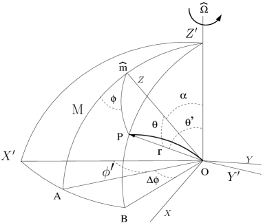
Figure 1: A schematic picture that depicts the geometry associated with the emission region. The $XYZ$ frame is co-rotating with the magnetic axis ${\hat{m}}$ around spin axis ${\hat{\Omega}},$ and the $X^{\prime}Y^{\prime}Z^{\prime}$ frame is the non-rotating frame of the observer.

In the $X^{\prime}Y^{\prime}Z^{\prime}$ coordinate system, the location of the emission spot can be specified by the values of $r,$ $\theta^{\prime}$ and $\phi^{\prime}_{\rm p}$ (see §A). The expressions for $\theta$ and $\phi$ are given in G04, and the expression for $\theta^{\prime}$ as a function of the pulsar rotation phase $\phi^{\prime}$ is given in G05. A point of emission on a dipolar field line can be expressed as $r=r_{\rm e}\sin^{2}\theta$. When rotation effects are not included, it turns out to be a trivial exercise to trace emission spots based on the expressions for $r(t),$ $\theta$ and $\phi$. For a given $\alpha$, $\beta$ and $S_{\rm L}$ combination, the value of $r(\phi^{\prime})=r_{\rm e}\sin^{2}[\theta(\phi^{\prime})]$, the radius of curvature $\rho$ can be readily found (Eq. 4 in G04). However, the estimation of $r$ and $\rho$ corresponding to the emission spot becomes difficult when the effects of rotation are included.

As mentioned before, when rotation is invoked, the observer will receive peak radiation when the particle velocity vector ${\hat{\textbf{v}}}$ (rather than the tangent to the field line) becomes parallel to the line-of-sight $\hat{n}$, where ${\hat{\textbf{n}}}=[\sin\zeta,0,\cos\zeta]$, and $\zeta=\alpha+\beta$. The total velocity of the charged particle will be the vector sum of the component parallel to the magnetic field, and the component in the azimuthal direction due to the co-rotation of the field (TG07). The component in the azimuthal direction will make the total velocity offset from the direction of the local field tangent. The analytical solution for the radial position of the trajectory of the charged particle, including the rotation effects, is derived in TG07. We employ the zeroth order solution that gives :

$$r(t)=\frac{c}{\Omega_{\rm m0}}\rm{cn}(\lambda-\Omega_{\rm m0}\,t)$$ (2)

where $\Omega_{\rm m0}=\Omega\sin\alpha,$ and $\rm cn(z)$ is the Jacobi Cosine function (Abramowitz & Stegun 1972), $\lambda$ is a constant, $t$ is the affine time and $c$ is the speed of light.

For a given $\alpha,$ $\beta$ and a rotation phase $\phi^{\prime}$, the radial distance for an emission spot can, in principle, be found by solving Eq. (1). The rotation phase $\phi^{\prime}$ is defined as the projected angle on the azimuthal plane between ${\hat{\textbf{n}}}$ and $\hat{\textbf{m}}$ (see Eq. (17) in §A). The above-said analytical expressions for the coordinates of the accelerated charged particle are to be as invoked as functions of affine time. The aberration phase shift $\delta\phi_{\rm aber}$ needs to be known in advance for solving Eq. (1) and finding the emission altitude, since the angles $\theta$ and $\phi$ are aberrated due to the rotation (see G05 for details, including the analytical expression for $\delta\phi_{\rm aber}$). Nonetheless, the emission altitude is apriori required for estimating the $\delta\phi_{\rm aber}$, thus making the problem non-linear. An analytical solution for Eq. (1) is nearly impossible owing to the bulky trigonometric terms. Approximations like $\delta\phi_{\rm aber}\approx r/r_{\rm L}$, will severely limit the expected precision of the solution. A straight forward numerical solution for Eq. (1) also encounters more or less similar difficulties owing to the aforesaid reasons. Hence we have developed special algorithms which are applicable for solving Eq. (1) under such conditions. We have devised an ‘exact’ method and also an ‘approximate’ method to compute the location of possible emission spots, which are suited for specific parameter regimes. These are described below.

3.2.1 The ‘exact’ method

For a ring of field lines specified by a field line constant $r_{\rm e}$ and for a given rotation phase $\phi^{\prime}$, we consider a point $P_{0}$ on a field line such that the unit-vector of the local field line tangent $\hat{\textbf{b}}_{0}$ is parallel to $\hat{\textbf{n}}$ in the non-rotating case. In the absence of rotation, the emission beam from the accelerated particles moving along the field line should be aligned with $\hat{\textbf{b}}_{0}$. But when the effects of rotation are invoked, the emission beam at $P_{0}$ gets mis-aligned with $\hat{\textbf{b}}_{0}$ and goes out of the line-of-sight. Hence the radiation from $P_{0}$ will not be received by the observer. However, another emission spot $P_{1}$ on the same ring of field lines can have the $\hat{\textbf{v}}$ parallel to $\hat{\textbf{n}}$ and contribute emission in the direction of the observer. Hence the observer will receive radiation from $P_{1}$ provided Eq. (1) is satisfied for $P_{1}.$ Let the aberration phase shift at $P_{1}$ be $\delta\phi_{\rm aber}$; then the updated values $\theta=\theta(\phi^{\prime}+\delta\phi_{\rm aber})$ and $\phi=\phi(\phi^{\prime}+\delta\phi_{\rm aber})$ at the point $P_{1}$ so that the emission is aligned with the line of sight to the observer (G05).

Hence the basic idea that is invoked in the computation of the exact method can be briefed as: for a given $\phi^{\prime},$ begin with the value of the emission height, which is estimated in the non-rotating case, and find the trial value of $\delta\phi_{\rm aber}$. Then solve Eq. (1) numerically to find an improved value of emission height. Continue the iteration till the solution for Eq. (1) satisfactorily converges. The main steps of algorithm are briefly described below :

1. Choose a specific combination of $\alpha,$ $\beta,$ $\gamma,$ $r_{\rm e}$ and $\omega,$ and a fixed rotation phase $\phi^{\prime}.$

2. Make the first estimate for the aberration angle $\delta\phi_{\rm aber}$ using the trial input values of $\theta(\phi^{\prime}),$ $\phi(\phi^{\prime})$ and $r,$ which follows from $r=r_{\rm e}\sin^{2}\theta(\phi^{\prime})$.

3. Using the $\delta\phi_{\rm aber}$ estimated above, the angles $\phi$ and $\theta$ are re-calculated with the rotation phase incremented by $\delta\phi_{\rm aber}.$ Henceforth update: $\phi(\phi^{\prime})\rightarrow\phi(\phi^{\prime}+\delta\phi_{\rm aber})$ and $\theta(\phi^{\prime})\rightarrow\theta(\phi^{\prime}+\delta\phi_{\rm aber})$.

4. Estimate $\bf v$ and hence the unit vector ${\hat{\textbf{v}}}={\bf v}/|{\bf v}|$ with the angles $\phi$ and $\theta,$ found in step 3.

5. Estimate the affine time ‘t’ that satisfies the matching condition ${\hat{\textbf{n}}}\cdot{\hat{\bf v}}=1$. Hence find the improved value of $r(t).$

6. Recalculate $\delta\phi_{\rm aber}$ with $r=r(t)$ and repeat the calculation from step 3 till convergence is achieved for ‘t’.

7. Using the improved value of $r(t)$ find $\bf v$, $\bf a,$ and $\rho.$

8. Using the $\rho$ estimate the spectral intensity.

9. Find the angle $\eta_{\rm mis}=\cos^{-1}({\hat{\textbf{n}}}\cdot{\hat{\textbf{v}}}).$

We choose to call this method as ‘exact method’ since the computation employs the exact expressions for the relevant quantities. The explicit expressions for magnetic co-latitude $\theta$ and magnetic azimuth $\phi$ are given by Eq. (25) and Eq. (26), respectively, in §A. The expressions for velocity v and acceleration a are given by Eq. (7) and Eq. (8) respectively, and the expression for radius of curvature $\rho$ is given in Eq. (28). Sample results from this method are shown in the figures in §C. The angle $\eta_{\rm mis}$ gives the residual difference between the line-of-sight and the estimated v at the end of the iterations. It’s ideal value is zero and hence, the final residual value obtained is a measure of the precision of the solution : a smaller value of $\eta_{\rm mis}$ indicates a more precise determination of the emission spot.

3.2.2 Alternative or ‘approximate’ method

We have devised an alternative or approximate method, for the estimation of $r$, $\rho$ and the related quantities, in cases where we encounter ‘extreme’ values of parameters. Such regimes are often combination of large values of $\alpha$, very low values of $\beta,$ and field lines close to magnetic axis ($S_{L}<0.5)$. The exact method encounters difficulties for such regimes in that the numerical solutions of Eq. (1) for affine time ‘t’ often do not give satisfactory convergence. So we resort to an approximate method that is suitable for this regime. By this method, we expect to determine the emission height and the radius of curvature with comparable precision to the exact one, for leading and the trailing parts of the pulsar profile. The estimates of this method have been optimised by comparison with the estimates of the aforesaid exact method in a common parameter regime where both the methods give reliable results. The scheme of the approximate method is: for a given rotation phase $\phi^{\prime},$ first calculate $r,$ $\theta$ and $\phi$ in the non-rotating case, and then use it to find approximate values of $r,$ $\theta$ and $\phi$ in the rotating case. The details are provided in §B.

3.3 Computing the intensity profiles

As explained earlier, we sweep the line of sight through discrete rotation phases, and using the afore-said steps given in §3.2.1 and §3.2.2, we find the parameters like emission altitude $r$, and the radius of curvature of the particle trajectory, $\rho$. Then we estimate the spectral intensity for a given frequency, $\omega$, for particles for a given Lorentz factor, $\gamma$, by using the standard curvature radiation formula (e.g. Jackson 1972) :

$$d\,I/d\omega~{}=~{}\sqrt{3}\frac{e^{2}}{c}\gamma\,\,u\int^{\infty}_{u}K_{5/3}(u^{\prime})du^{\prime}~{},$$ (3)

where $u={\omega}/{\omega_{\rm c}}$ and the characteristic frequency $\omega_{\rm c}=1.5\,\gamma^{3}\,c/\rho$. According to Eq. (3), the spectral-intensity curve should peak at $u=0.286$, which corresponds to $\rho/\rho_{\rm p}=1$, where the parameter $\rho_{\rm p}$ can be defined as

$$\rho_{\rm p}=0.286\times 1.5\gamma^{3}\frac{c}{\omega}~{}.$$ (4)

Invoking this parameter helps in easy identification of the peak points in the spectral-intensity plots.

An important feature of this method is that it computes the contribution to the observed intensity for any frequency $\omega,$ different from $\omega_{\rm c}.$ Often in literature, significant contribution of intensity to the observer is presumed to be concentrated near the characteristic frequency $\omega_{\rm c}=1.5\gamma^{3}c/\rho$, thus providing an in-built frequency selection criteria (e.g., Melrose 2006). However, the spectral intensity curve for curvature radiation has non-negligible amount of power emitted at a significant range of frequencies different from $\omega_{\rm c}.$ Our formulation thus allows for a more complete treatment of the amount of emitted intensity and its reception by the observer.

Since our present analysis necessitates only the computation of relative intensities of the simulated profiles, invoking a single particle emission model for the curvature emission do not alter the results in a significant manner. The high luminosity of the pulsars demands imposing coherence on the emission, perhaps in the form of bunched emitting sources, and the process behind the formation of such bunches is still being investigated. In a simple manner, coherent emission from a bunch with charge Q can be alternatively expressed as the emission from a single particle with the same charge Q. So, the relative intensities are not affected by this simplification and hence considering single particle emission do not tamper with the physics behind the emission. Further discussions regarding this factor will be followed in later sections.

3.4 Typical outputs

We have computed the parameters of emission in the magnetosphere by implementing the method described above. The free parameters are the following : $\alpha$, $\beta$ (pulsar geometry), $\Omega$ (pulsar rotation frequency), $\gamma$ (Lorentz factor of the particles), $S_{\rm L}$ (field line location) and $\omega$ (radio frequency of observations). For the sake of brevity of presentation, we give results for a single fixed value of $\Omega=2\pi$ (i.e. a spin period of 1 sec), and for a relatively narrow range of rotation phases of about $-10^{\circ}$ to $+10^{\circ}$ around zero (fiducial) phase. As is discussed later, frequency turns out to be a relatively weak parameter in comparison to other strong ones that influence profile evolution. Hence, for the simplicity of analysis, we have restricted the frequency to a single value of 610 MHz. For a chosen pulsar geometry, the emission locations are estimated for each discrete rotation phase and for a set of discrete choices of $S_{\rm L}.$ Further, the specific intensity values are estimated for a set of discrete values of $\gamma$, for a fixed value of $\omega.$

The typical outputs are shown in the figures in §C. Fig. 4 shows the basic outputs from a typical simulation run for estimating the location of emission regions, for a fixed pulsar geometry, for a set of $S_{\rm L}$ values (0.1, 0.3, 0.5 and 0.7). The following quantities are shown, as function of rotation phase, in separate panels for each $S_{\rm L}$ value : the estimated emission altitude, $r$; the computed radius of curvature of the particle trajectory, $\rho$; the $\phi$ and $\theta$ for the emission spots in the magnetosphere; and the mis-alignment angle, $\eta_{mis}$, which is a measure of the accuracy of the results. Fig. 5 shows the computed intensity profiles for each choice of $S_{\rm L}$ values (in separate panels) for a set of $\gamma$ values (200, 300, 400, 600, 1000, 1500), for a fixed observation frequency of 610 MHz. These two figures illustrate the basic results. The effect of varying pulsar geometry can now be explored to understand the variety of intensity profiles that are possible. Most important outputs are $r/r_{\rm L}$, $\rho/r_{\rm L}$ and specific intensity plots, and the successive figures show only these quantities.

Figures 6 to 10 then investigate the effects as a function of pulsar geometry (i.e. different combinations of $\alpha$ and $\beta$ values), with the range of $S_{\rm L}$ values and $\gamma$ values confined to those illustrated in Figs. 4 and 5.

4 Results and discussion

4.1 General results

We first discuss the general results and trends that are deduced from our simulation studies, as illustrated in the results displayed in the plots given in §C.

4.1.1 Emission heights

The heights for the allowed emission spots have a minimum value near the magnetic meridian ($\phi^{\prime}=0$), with smoothly increasing values on the leading and trailing sides. However, the variation of height with rotation phase is asymmetric such that the increment with rotation phase is always faster for the trailing side than for the leading side. Whereas this increase with rotation phase is purely geometric, the asymmetry in this is due to the modification of particle trajectories produced by rotation. On the leading side, the emission beam bends in the direction favourable to rotation and hence advances in azimuthal phase by $\delta\phi^{\prime}_{\rm aber}$ from that of the corresponding field line tangent. Hence at a fixed $\phi^{\prime},$ an emission spot located at a lower emission height than in the non-rotating case will satisfy Eq.1. In contrast, on the trailing side, the bending of the emission beam causes a lag in azimuthal phase by $\delta\phi^{\prime}_{\rm aber}$ from the corresponding field line tangent. This lag can be compensated by an emission spot located at a different altitude than the non-rotating case. Hence an emission spot located at a different emission height will satisfy Eq.1 and contribute radiation to the observer.

Both the value of the minimum height (at $\phi^{\prime}=0$), as well as the asymmetry, are larger for the inner field lines as compared to the outer field lines. This supports the intuitive expectation that outer field lines would be visible out to much larger pulse longitude ranges than inner field lines. Further, it is seen that the minimum height and asymmetry of the variation increase with geometry, being more for larger values of $\alpha$ and $\beta$. Also, pulsars with larger values of $\alpha$ will have a larger range of variation of allowed emission heights, for the same field line. It is reasonable to surmise that a similar value of emission height can be seen recursively for several combinations of larger and smaller values of $\alpha$ and $S_{\rm L},$ for a certain $\phi^{\prime}$. Thus we find that the values of $\alpha$ and $S_{\rm L}$ dominantly decide the range of emission heights. Even otherwise, the $\alpha$ dependence of the emission height can be directly understood from Eq.(2), since the expression $r(t)$ is explicitly dependent on the value of $\alpha.$

4.1.2 Radius of curvature

The radius of curvature inferred for the possible emission spots also varies signficantly with rotation phase, and it is significantly asymmetric between leading and trailing sides. If rotation effects were not considered, this radius of curvature would be same as that of the corresponding field line and be symmetric around zero pulse phase. Given that the observed radius of curvature of the particle trajectory is a combination of the curvature of the field line and curvature introduced due to rotation, the observed asymmetry is a rotation effect and can be understood as a combination of two effects: first, as the allowed heights are different on the leading and trailing sides (for the same phase $\pm\phi^{\prime}$ on either side of the zero phase), the radius of curvature of the field line itself would be different; second, on the leading side, the curvature of the field line gets combined with that induced by rotation (TG07), resulting in a lower value of the $\rho$ for the particle trajectory. Whereas on the trailing side, the two curvatures are opposed and hence the net curvature is reduced, leading to larger values of $\rho.$ In fact, for some field lines, rotation induced curvature can cancel the curvature due to the field lines, at some points on the trailing side, resulting in sharply peaked curves for $\rho$ for certain values of $S_{\rm L},$ as seen in the plots in Figs. 7, 8 & 9. The variation of $\rho$ on the leading side is more or less steady, while on the trailing side it often varies very rapidly due to the aforesaid reasons.

The trend is that the asymmetry seen in $\rho$ will be higher for larger values of $\alpha$ and smaller values of $S_{\rm L}$ and hence it is a combined effect of both. As mentioned earlier, the rotation effects are more at higher $\alpha$ and hence the larger asymmetry. Since the range of emission altitudes covered by the emission spots for inner field lines are higher than that of the outer field lines, the corresponding values of $\rho$ also will have a higher range and a higher asymmetry than the ones for the outer field lines. However, there are variations in the amount of asymmetry with in the field lines when the $\alpha$ varies, and hence a steady variation of asymmetry with $\alpha$ will not be observed as for the emission heights.

Comparing the $\rho/\rho_{\rm L}$ plots for figs. 8 & 9, we can find on the leading side that the radius of curvature gets reduced when $\alpha$ increases from $60^{\circ}$ to $90^{\circ}$ for all field lines. But on the trailing side the behaviour is slightly different. The inner field lines ($S_{\rm L}=0.1~{}\&~{}0.3$) have the radius of curvature slightly reduced on the trailing side, while an increment in radius of curvature is seen for outer field lines ($S_{\rm L}=0.1~{}\&~{}0.3$), when $\alpha$ increases from $60^{\circ}$ to $90^{\circ}.$ Another comparison of the $\rho/\rho_{\rm L}$ plots for the figs.  4  &  8 obviously shows the same trend for the leading side. However, the variation of $\rho/\rho_{\rm L}$ on trailing side shows a slightly different behaviour, varying among field lines. The variation of $\rho$ on the trailing side is not in a steady pattern as on the leading side. The competing curvatures due to rotation induced curvature and the intrinsic field line curvature gives a highly varying pattern for $\rho$ on the trailing side.

4.1.3 Spectral Intensity, $I_{\omega}$

The derived spectral intensity curves reflect the asymmetry inherited from the variation of $\rho$ with pulse phase, combined with the effects of the value of $\gamma$. In particular, it is readily seen that the intensity dramatically evolves with $\gamma.$ For lower values of $\gamma$, the $I_{\omega}$ has a stronger leading part while for higher values of $\gamma$ the $I_{\omega}$ has a stronger trailing part. This effect can be better understood by considering the parameter $\rho_{\rm p}$ (defined in Eq. (4)), which gives the value of $\rho$ at which the spectral intensity peaks, for given values of frequency and $\gamma$. For values of $\rho$ greater than or less than $\rho_{\rm p}$, the spectral intensity falls monotonically. Further, the peak value of the spectral intensity also depends on the specific value of gamma, as per Eq. (3). Hence, the variation of spectral intensity with pulse longitude can be inferred from that of $\rho$ with longitude, for different values of gamma. This is illustrated in fig.  5 where $\rho/\rho_{\rm p}$ and the corresponding $I_{\omega}(\phi^{\prime})$ are plotted side by side as a function of the rotation phase, for specific combinations of parameters.

Three different cases are useful to consider. For situations where $\rho/\rho_{\rm p}$ is greater than 1.0 for the entire pulse window, the spectral intensity curve shows a maximum at $\phi^{\prime}=0$ and falls asymmetrically on either side, with the reduction in intensity being larger for the trailing side, due to the faster increase of $\rho$. This effect, which is seen for relatively small values of $\gamma$ (less than 400-600), naturally leads to asymmetric pulse profiles, with possibilities for sharply one-sided profiles. It is interesting to note that in some cases, the intensity on the trailing side can drop to negligible values, compared to its value at the corresponding longitude on the leading side. This could be a natural explanation for the one-sided cones reported in literature, and is discussed in more detail in §4.6.

For situations where $\rho/\rho_{\rm p}$ is less than 1.0 for the entire pulse window, the spectral intensity curve shows a minimum at $\phi^{\prime}=0$ and rises asymmetrically on either side, with the increase being larger on the trailing side. However, the contrast in the intensity levels between leading and trailing sides is typically not as high as for the first kind. This behaviour is seen for relatively large values of $\gamma$.

For intermediate cases, where values of $\rho/\rho_{\rm p}$ less and greater than 1.0 can occur at different points in the pulse longitude window, we see more complicated shapes for the spectral intensity curves, including multiple maxima at different pulse longitudes.

For a given geometry and $s_{\rm L}$ value, the transition through these 3 different cases can take place as $\gamma$ is varied over a range of values. Thus, lower values of $\gamma$ tend to produce profiles with strong leading and weak trailing intensities which get converted to weak leading and strong trailing kind as the $\gamma$ increases to very high values (e.g. 2nd and 3rd panels from the top in fig. 5). Though the contrast in intensity is less for the latter, the absolute value of the spectral intensity is higher, due to the $\gamma$ dependence in Eq. (3).

Most of the asymmetric intensity profile effects become more dramatic for inner field lines and for more orthogonal rotators (larger $\alpha$) and smaller values of $\beta.$

4.1.4 $\theta$ and $\phi$

The values of $\theta$ and $\phi$ are asymmetric on the leading and the trailing sides of the profiles, while they are symmetric in the non-rotating case (G04). This asymmetry is also an effect of rotation. Since $\theta$ and $\phi$ are functions of $\phi^{\prime}$ their values are affected by the aberration phase shift which is different on leading and the trailing sides. Their values are dominantly decided by $\alpha$ and $\beta$. As expected, the shape of the $\phi$ curve closely resembles the S-shape of the polarization angle curve (see fig. 4).

4.1.5 Mis-alignment angle, $\eta_{\rm mis}$

The Mis-alignment angle $\eta_{\rm mis},$ defined as $\eta_{\rm mis}=\cos^{-1}({\hat{\textbf{n}}}\cdot{\hat{\textbf{v}}}),$ gives an estimate of the offset between $\hat{\textbf{n}}$ and the estimated $\hat{\textbf{v}}.$ In principle, for a perfect estimation of the emission point, the line of sight should exactly coincide with the velocity vector, and hence $\eta_{\rm mis}$ should be zero. However, in actual computations, $\eta_{\rm mis}$ always has a small, finite value. A quick check of the accuracy of the computation is provided by the value of $\eta_{\rm mis}$ : a lower value implies a higher precision of estimation of the emission spot, and vice versa for a higher value. A rough classification that can be taken for the precision of the estimation is: a value of $\eta_{\rm mis}\ll 1$ indicates a highly precise estimation of the emission spot, and vice versa for $\eta_{\rm mis}\gg 1.$ By this scheme, we find that there is satisfactory precision for all estimations for $r$ within 20 % of $r_{\rm L}$ (see fig. 11). In some cases the $\eta_{\rm mis}$ exceeds 1, but only when $r/r_{\rm L}>0.2.$ However, according to established observational results radio emission heights are restricted within 10 % of $r_{\rm L}$ for normal pulsars (e.g. Kijak 2001), and hence our method is quite satisfactory in this regime of interest.

4.2 Effects of Parameters

The above described behaviour of the height of emission spots, radius of curvature and spectral intensity are strongly dependent on the parameters like geometry, field line location, radio frequency and Lorentz factor of the particles. In some cases, there is a complex interplay between the dependencies on these different parameters. Here, we explore some of these effects in detail.

The generic effects of $\gamma,$ $\alpha$ and $\beta,$ $\omega$ and $S_{\rm L}$ are listed briefly below in an order that may characterize the hierarchy of their effects on total intensity profiles.

4.2.1 Inclination angle, $\alpha$

The parameter $\alpha$ is a major driver of the effects of rotation, and has the strongest influence on our results and conclusions. The rotation effects (leading-trailing asymmetry of $r,$ $\rho$ and $I_{\rm\omega}$) are more prominent for large values of $\alpha$ and less for small values of $\alpha.$ The range of emission altitudes is found to be relatively high for lower values of $\alpha$, and relatively low for higher values of $\alpha,$ being the lowest for $\alpha=90^{\circ}.$ Like wise, $\rho$ appears to reach higher values for higher $\alpha$ and vice versa for lower $\alpha.$

4.2.2 Normalized foot value of the field lines, $S_{\rm L}$

The effect of moving from inner to outer regions of the magnetosphere (increasing $S_{\rm L}$ values) also has a very dramatic effect on the results. Rotation effects are strongest for the innermost field lines, and decrease significantly for larger $S_{\rm L}$ values. For relatively small values of $S_{\rm L}$ (usually $\leq$ 0.3), the leading part has emission heights that vary relatively gently with $\phi^{\prime}$, whereas the trailing part shows steeply rising emission height. The emission heights become less asymmetrical for increasing values of $S_{\rm L}.$ The values of $\rho$ steadily increase with decreasing $S_{\rm L}$ (i.e. inner field lines) on the trailing side. Dramatic effects such as very large, peaked values of $\rho$ on the trailing side, owing to the mutual cancellation of intrinsic and rotation induced curvatures, are seen only on inner field lines. This peak shifts closer towards zero pulse phase as the value of $S_{\rm L}$ becomes smaller. For outer field lines, the profiles are much more symmetric, and since $\rho/\rho_{\rm p}<1$ for a significant range of pulse phase on either side of $\phi^{\prime}=0$, the profiles more often exhibit minima at $\phi^{\prime}=0$, even for moderate values of $\gamma$.

4.2.3 The lorentz factor, $\gamma$

The effect of $\gamma$ has a very clear signature on the asymmetry of the spectral intensity profiles. For lower values of $\gamma$, there can be strong asymmetries with leading side stronger than the trailing side, and maxima at $\phi^{\prime}=0$. For larger values of $\gamma$, the sense of this asymmetry can reverse, with trailing side becoming stronger than the leading, and a minima at $\phi^{\prime}=0$ ; however, the degree of the asymmetry, as measured by the ratio of the intensities at corresponding longitudes, is generally less than that for the case for the low $\gamma$ values.

4.2.4 Emission frequency, $\omega$

The frequency of emission, $\omega$, acts as a counter to the effect of $\gamma$, though in a relatively weak manner, as can be understood from Eqs.  (3) and  (4). Thus, an increase in $\omega$ produces changes which can be compensated by a corresponding change in $\gamma$ by a factor proportional to $\omega^{1/3}$. In certain cases, this could result in profiles where the sense of asymmetry between leading and trailing sides could reverse over a large enough range of radio frequencies. Such effects are seen sometimes in some real profiles.

4.3 Realistic profiles

One of the significant results from our simulation studies is that the possible regions of emission associated with a given annular ring of field lines (characterised by a constant value of $S_{\rm L}$) are visible over a wide range of pulse phase, albeit with different intensity levels. This aspect, combined with the results for field lines with different values of $S_{\rm L}$, leads to the conclusion that a very large fraction of the pulsar magnetosphere is potentially visible to us. This results in simulated pulsar profiles that are very different from the observed profiles of real pulsars which appear to have well defined emission components, restricted in pulse phase extent to occupy only some fraction of the on-pulse window. This disparity with the observed profiles persists even after we incorporate into our simulations the models of discrete, annular conal rings of emission.

Hence, in order to reproduce realistic profiles matching with observations, we need some additional constraints for the emission regions. In the most general case, such non-uniformities in the distribution of emission regions can exist in any of the three coordinate directions, viz. $r$, $\theta$ and $\phi$. Non-uniformity of emission in the $\theta$ direction is achieved in some sense at the basic level, by considering only discrete sets of $S_{\rm L}$ values for active emission regions. As discussed, this is not enough to constrain the intensity variations to reproduce realistic pulsar profiles.

The possibility of non-uniform emission along the $\phi$ coordinate could help produce discrete emission components in the observed profiles. As seen in fig.  4, for a given value of $S_{\rm L},$ the emission at different pulse longitudes originates at widely different $\phi$ locations. If the sources of charged particles were located only at fixed $\phi$ points along the ring of constant $S_{\rm L},$ then these could be arranged to modulate the simulated intensity pattern with a suitable “window” function, to obtain discrete emission components in the observed profile. However, the well known phenomenon of sub-pulse drift argues against this being a viable option. Sub-pulse drift, which is now believed to be fairly common in known pulsars (e.g. Velterwede et al. 2006), wipes out any azimuthal discretization of sources of emission in the pulsar magnetosphere – it would lead to “filling up” of the intensity average profile over a given range of pulse longitude, as is observed in drifting sub-pulses that occur under any discrete emission component in known pulsars.

The third option is to have non-uniform emission in the radial direction, i.e. preferred heights of emission for a given set of field lines. Since the contributions at different pulse phases are from different heights, this would naturally lead to non-uniform distribution of intensity in pulse phase, resulting in realistic looking pulse profiles. The idea of preferred heights of emission in the pulsar magnetosphere is not entirely new – the “radius to frequency mapping” model for pulsar emission postulates different heights for different frequencies, with the height of emission increasing for decreasing frequency values (Kijak & Gil 1997,1998; GG01, GG03).

Figure 2: PSR B2111+46 at 333 MHz : The emission height for each $S_{\rm L}$ value associated with a particular component is plotted in panel (a). The simulated and un-modulated spectral intensity curve corresponding to each $S_{\rm L}$ value is plotted in panel (b). The simulated sub-components, after applying Eq.(6) for the best fit values given in Table.1 are shown in panel (c). The sum-total of the simulated sub-components giving the final profile (solid curve) is shown superposed with the observed profile (dotted curve) in panel (d).

Preferred emission heights of emission with a spread in the $r$ direction, can be modeled as a multiplication of the spectral intensity ${I}_{\omega}(\phi^{\prime})$ with a modulating function, $F^{\rm i}_{\omega}(\phi^{\prime})$. For modelling a profile as a sum total of emissions from a core and several discrete conal regions, the modulated spectral intensity can be expressed as

$${I}_{\omega}(\phi^{\prime}) = \sum_{i}^{N}{I}^{\rm i}_{\omega}(\phi^{\prime})\,\,F^{\rm i}_{\omega}(\phi^{\prime})~{},$$ (5)

$$F^{\rm i}_{\omega}(\phi^{\prime}) = A^{\rm i}_{\omega}\exp\left[-\left(\frac{r^{\rm i}_{0}(\phi^{\prime})-H^{\rm i}_{\omega}}{2\,\Delta H^{\rm i}_{\omega}}\right)^{2}\right]~{},$$ (6)

where the index $i$ represents, a corresponding pair of leading-trailing components presumed to be arising from a particular ring of field lines; while $i=1$ exclusively represents the central core component. Here $N$ is the total number of such discrete emission components (for example, $N=3$ would correspond to a 5 component profile forming a central core and two pairs of conal components), ${I}_{\omega}(\phi^{\prime})$ is the total spectral intensity from all field lines combined, while ${I}^{\rm i}_{\omega}(\phi^{\prime})$ is the spectral intensity from the $i$th ring of field lines. For a given emission region, $H^{\rm i}_{\omega}$ represents the mean height, and $\Delta H^{\rm i}_{\omega}$ represents the spread of the region. The variable $r^{\rm i}_{0}(\phi^{\prime})$ represents the values of emission altitude for each value of $\phi^{\prime}$ estimated by the simulation method as described earlier, for the $i$th ring of field lines.

To map this intensity as a function of rotation phase as seen in the observer’s frame, the effects of retardation and aberration need to be included explicitly. The effect of aberration is estimated by default and the $\phi^{\prime}$ is inclusive of the aberration phase shift. The retardation phase shift is to be estimated from the value of $r$ corresponding to the emission spot. The rotation phase corresponding to ${I}_{\omega}$ is updated after adding the retardation phase shift $d\phi^{\prime}_{\rm ret}$ with $\phi^{\prime},$ and this is represented by the mapping of the ordered pair $(\phi^{\prime},{I}_{\omega})\rightarrow(\phi^{\prime}+d\phi^{\prime}_{\rm ret},{I}_{\omega}).$ The $d\phi^{\prime}_{\rm ret}$ can be estimated as (G05) :

$$d\phi^{\prime}_{\rm ret}=\frac{1}{r_{\rm L}}({\vec{r}}\cdot{\hat{n}}),$$

where ${\vec{r}}=r{\hat{e}}_{\rm r}$ and the expression for ${\hat{e}}_{\rm r}$ is given in §B. The height of emission ($H^{\rm i}_{\omega}$) and the normalized foot value ($S^{\rm i}_{\rm L}$) corresponds to the peak of the $i$th component of the profile. The $\Delta H^{\rm i}_{\omega}$ and $A^{\rm i}_{\omega}$ are model parameters.

Table 1: The parameters for simulating the profiles of PSR B2111+46

Frequency	${\rm i}^{a}$	$H^{i}_{\omega}$	$\Delta H^{i}_{\omega}$	$A^{i}_{\omega}$	$S_{\rm L}$	Lorentz factor
MHz		Km	Km			$\gamma$
333	1	1500	600	1.8	0.08	750
	2	1834	500	0.14	0.18	750
	3	3800	500	0.7	0.3	500
408	1	300	850	2.2	0.09	750
	2	1200	750	0.1	0.22	750
	3	3000	400	0.9	0.35	500
610	1	200	700	1.7	0.13	750
	2	500	450	0.3	0.31	700
	3	2600	500	1.5	0.35	550

^a $i=1$ represents the core component,
$i=2$ represents the inner conal component,
$i=3$ represents the outer conal component.

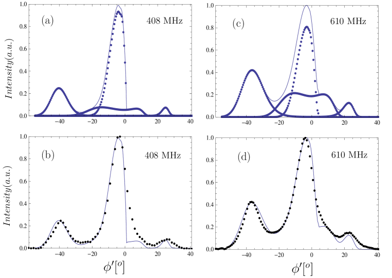
Figure 3: PSR B2111+46 at 408 & 610 MHz: In panels (a) and (c) , the dotted curves shows the simulated sub-components and the continuous curve shows their sum-total. In panels (b) and (d), this final simulated profile (solid curve) is superposed with the observed profile (dotted curve).

4.4 Profiles for PSR B2111+46 : a test case

Using the afore said methods for simulation of pulse profiles, we have attempted to reproduce the intensity profiles of PSR B2111+46 obtained from EPN data base and GMRT data, at multiple radio frequencies. This pulsar has a multi-component profile, with a well identified core component and 2 cones of emission (e.g. Zhang et al. 2007). It has a rotation period of 1.014 sec and $\alpha=14$ and $\beta=-1.4$ (Mitra & Li 2004). The other parameters used in the simulation are listed in Table 1. The values of emission heights $H^{\rm i}_{\omega}$ and field line locations $S^{\rm i}_{\rm L}$ for the discrete emission components are the values from estimates employing the method given in Thomas and Gangadhara (2009). The zero phase of the profile is fixed on the basis of the analysis of core emission of this pulsar, using the method developed in the the same work.

The simulation method is illustrated in fig. 2. Values of $S_{\rm L}$ corresponding to the core and conal components are employed in generating the emission height plots in panel (a) of fig. 2. The corresponding spectral intensity plot for each of these $S_{\rm L}$ values, for the final best fit choice of $\gamma$ (in Table 1) is shown in panel (b) of this figure. The individual components generated after applying the best fit height function are shown in panel (c) and the sum total intensity profile is shown in panel (d), along with the observed profile. Best fits of these profiles to the observed data were obtained by varying $A^{\rm i}_{\omega}$ and $\Delta H^{\rm i}_{\omega}$ in the function $F^{\rm i}_{\omega}(\phi^{\prime})$, and by varying the value of $\gamma$ in the range 100 to 1000. The same procedure is repeated for 408 MHz and 610 MHz profiles and the results are shown in fig. 3. All the final parameters and best-fit results are summarised in Table.1.

An encouraging first order match between the simulated and observed profiles has been achieved (see panel (d) of fig. 2 & panels (b) and (d) of fig. 3). The core component is quite well fit for most of the cases, and so are the leading conal components. There is some mismatch in the widths of the conal components, especially for the trailing side, where the real data shows a smoother blending of the components, compared to the simulated profile where the components appear more narrow and relatively well separated. It is remarkable that with a single value of $A^{\rm i}_{\omega}$ for a leading-trailing pair of cones of emission, the ratios of the peak values of the intensity of the leading and trailing components of the cones match so well with the real data. It is also interesting to note that the best fit values for $\gamma$ are very similar for a given emission component, at different frequencies, supporting a model of a common bunch of accelerated charged particles being responsible for the emission at different frequencies. Further, that the spread of $\gamma$ values across the different emission components is also quite small, indicates very similar operating conditions over most of the magnetosphere. The best fit values for $\Delta H^{\rm i}_{\omega}$, though reasonable, are somewhat large in amplitude, indicating somewhat extended emission regions in the magnetosphere.

We note that these relatively large values of $\Delta H^{\rm i}_{\omega}$ and some of the limitations of the fits may be due to the lack of some generalizations in our model. These include factors like coherency of emission, a realistic spread of $\gamma$ values around the mean values obtained here, as well as a realistic spread in the values of $S_{\rm L}$ due to finite thickness of the rings of emission on the polar cap. Whereas a detailed treatment of all of these is beyond the scope of this work and will be taken up later, some basic inferences can still be drawn. For example, if a small range of $S_{\rm L}$ values around the mean is considered, it is easy to argue that much of the width of a profile component can be filled up by radiation from such a bunch of field lines. This can be understood from panel (a) of fig.  2, where a line of constant height intersects the curve for a given field line at two points, one each on the leading and trailing side. The phase of this point of intersection will move systematically as we go to neighbouring field lines. Hence, wider profile components can be achieved with smaller values of $\Delta H^{\rm i}_{\omega}$. Furthermore, due to the asymmetry in the emission height curves, the shift in phase with change of $S_{\rm{}_{L}}$ is more on the trailing side, which would naturally lead to broader component widths and better ‘blending’ of the components in the profile, something that is not as easily achievable by having a large range of emission heights (as the shift of phase for a given separation of heights on a given field line is lesser on the trailing side). One indicator of the significance of the spread of $S_{\rm{}_{L}}$ values is the amount by which $S_{\rm{}_{L}}$ needs to be changed to move the peak of one conal component to the point half-way to the peak of the next conal component. Not very surprisingly, our rough estimates show that the required change in $S_{\rm{}_{L}}$ is close to the half-way point to the $S_{\rm{}_{L}}$ value of the next cone, which would indicate a closely packed structure of concentric rings.

The component profiles could be further influenced by considering a distribution of $\gamma$ values associated with the emitting particles. We have found that significant shifts in the peaks of the leading and trailing pair of components for simulated profiles are obtained for lower $\gamma$ values ($\gamma<500$), while the peak positions appear almost frozen for increasing $\gamma$ values. Thus it is realistic to assume that a spread of $\gamma$ values can broaden the emission components. This factor also may reduce the $\Delta H^{\rm i}_{\omega}$ required to effect a good fit.

Nevertheless, we would like to point out that there is only one unique combination of the parameters that can produce a profile which is similar to the observed one. We have not found any degenerate combination of values for the parameters that are shown in Table.1. Thus, the similarity of the simulated profiles with the observed ones gives an assurance that, we should be able to simulate the observed profiles with greater similitude with a model overcoming the above-said limitations.

4.5 Core emission

The generation of the profile components for PSR B2111+46 described above naturally leads to a discussion on the core emission. In fact, the study of the phenomena of core emission has spawned enormous amount of literature. Perhaps the most notable ones are the landmark work by Rankin (1983) that systematized the pulsar emission profile into ‘core’ and ‘cone’, and the succeeding works by Rankin (1993a & 1993b) that further developed the core-cone classification scheme. The hollow cone model was invoked to explain the geometry (e.g. Taylor & Stinebring 1986) and the origin of core emission. Radhakrisnan and Rankin (1990) have conjectured that the emission mechanism for cores might be different from that of cones, owing to the behaviour of polarization position angle curve near the core being different from the rotating vector model. However, there are no satisfactory theoretical grounds for postulating diverse mechanisms for cores and cones. A major difficulty that curvature radiation encounters in explaining the core emission is the insufficient curvature of the almost straight field lines in a region relatively close to the pulsar polar cap. Since the intensity of emission is proportional to $1/\rho^{2}$, the values of $\rho$ provided by the intrinsic curvature of the field lines is too large and hence insufficient to generate enough intensity of emission typically observed for core component. This factor even prompted invoking other emission mechanisms for explaining core emission (e.g. Wang et al. 1989).

In our simulation studies, the presence of the core component comes about quite naturally. It can be seen from all the plots of spectral intensity in §C that the emission from regions near the profile centre is comparable (for higher $\gamma$ values) or even somewhat higher (for lower $\gamma$ values) than that from regions in the wings of the profile. This happens because we get low values of $\rho$ for inner field lines near $\phi^{\prime}\approx 0$, which are comparable to that of outer field lines, and this occurs consistently for all the combinations of $\alpha$ and $\beta$ (see the panels for $\rho/r_{\rm L}$ in §C). The reason is that rotation induces significant curvature into the trajectory of particles, even though they are confined to move along the nearly straight inner field lines.

The forces of constraint act in such a way that the particle is hardly allowed to deviate away from the field line on which it is moving, and the resulting scenario is discussed in detail in TG07. Due to the co-rotation of the field lines and the action of the aforesaid forces of constraint the charged particles are added with a velocity component in the direction of rotation, which is nearly perpendicular to the velocity component parallel to the field line, in the observer’s frame. This induces an additional curvature in the trajectory of the particle and makes it significantly different from that of the field line curvature in the observer’s frame of reference (TG07). Hence the trajectory of charge particles moving on almost straight field lines near the magntic axis can have a highly curved trajectory and hence a relatively low value of radius of curvature that is significantly different from that of the field lines. This scenario allows for significant emission near the central region of the profiles. By applying Eq. (5) and Eq. (6) appropriately, as described earlier, profile shapes resembling strong core components can be easily generated. Hence by applying our method, we provide a natural explanation for core emission, that circumvents the issue of too high $\rho$ that precludes a strong core component with curvature emission.

In the simulation of the profiles for PSR B2111+46, we find that the core originates from have relatively inner field lines and lower emission heights than the cones. Assuming the same mechanism of emission, viz. curvature radiation, for the core and conal component, we are able to produce a simulated core component that matches quite well with the observed profile. We notice that the best-fit values for the amplification factor $A^{i}_{\omega}$ found in the simulation for the core component (Table  1) are comparable to those of the cones. These values are not unduly high, considering the situation that the density of plasma should be relatively higher for the lower altitude and hence an additional factor for relatively stronger emission at lower altitudes. Our profile-matching of PSR B2111+46 thus shows that strong core emission can originate from inner field lines due to curvature emission.

4.6 Partial cones

According to LM88, partial cone profiles are the ones in which one side of a double component conal profile is either missing or significantly suppressed. These are recognised by the characteristic that the steepest gradient of the polarization position angle is observed towards one edge of the total intensity profile, instead of being located more centrally in the profile as the rotating vector model postulates. LM88 speculated that this happens when the polar cap is only partially (and asymmetrically) active. It is significant that, out of the 32 pulsars listed in LM88 that display the partial cone phenomena, as many as 22 have the steepest gradient point occurring in the trailing part of the profile. In other words, most of the partial cone profiles show a strong leading component and an almost absent trailing component.

Table 2: The parameter values employed in fig.10

Panel	$\alpha$	$\beta$	$S_{\rm L}$	$H^{i}_{\omega}$	$\Delta H^{i}_{\omega}$
No.	$[^{o}]$	$[^{o}]$		$Km$	$Km$
1	90	1	0.3	1000	200
2	90	1	0.5	1200	150
3	60	1	0.3	1000	200
4	60	1	0.5	1400	150
5	30	1	0.1	2500	500
6	30	1	0.3	1000	150

There are two possible scenarios that have been postulated to explain partial cones : (1) only a part of the polar cap is active (this works for both kinds of partial cones) or (2) the A/R effects are so large as to shift the entire active region of the intensity profile towards the leading side (this works for the strong leading type partial cones, which are the majority). However, Mitra et al (2007) studied several pulsars with partial cones with very high sensitivity observations and found that the almost-absent parts of the cones do flare up occasionally and show emission for about a few percentage of the total time. This tends to rule out both the scenarios above, and requires an explanation where the intensity is naturally suppressed in one side of the cone.

In our simulation studies, one sided cones appear as a natural by-product. We notice that for smaller values of $\alpha,$ inner field lines and lower $\gamma$ values, the intensity profile is almost always significantly suppressed on the trailing side, as compared to the leading side. The reason for this is quite obvious. As explained earlier, the $\rho$ for inner field lines is highly asymmetrical between the leading and trailing sides – it remains more or less steady on the leading side, while on the trailing side it shoots up to a high value and then falls. Whenever the $\rho$ shoots up such that $\rho/\rho_{\rm p}\gg 1$, the spectral intensity is significantly reduced. On the other hand, on the leading side we mostly have $\rho/\rho_{\rm p}\approx 1$ and hence the spectral intensity is significant there. For relatively lower values of $\gamma,$ $\rho_{\rm p}$ reduces and hence there is a greater chance of having $\rho/\rho_{\rm p}\gg 1$, while for higher values of $\gamma$, $\rho/\rho_{\rm p}$ drops down and eventually becomes closer to 1. Hence the intensity plots shown in §C are stronger on the leading side at low $\gamma$, and stronger on the trailing side at high $\gamma$. However, it is to be noted that (i) the values of $\gamma$ required to achieve stronger trailing side profiles are very high – usually significantly more than 1000; whereas, for more typical values of $\gamma$, we get the stronger leading side profiles and (ii) the intensity contrast obtained for the stronger leading side profiles is much larger and striking, compared to that for the stronger trailing side profiles. Both these facts argue naturally for a strong preponderance of one sided cones with stronger leading side profiles, as is statistically seen in the results of LM88.

To further illustrate the idea, we have generated profiles as shown in fig.  10 that resemble partial cone profiles by using our simulation technique for specific combinations of parameters, which are listed in Table  2. The thin line curve represents the un-modulated profile, which is simulated by assuming that the emission is uniform all along the field line, while the thick line shows the final modulated profile. The active region of the final profile is clearly shifted to the leading side, due to the afore said behaviour of $\rho.$ The suppression of the intensity on the trailing part in comparison to the leading side is seen in all the plots and is most dramatic for the inner field lines, for low values of $\gamma$, and for large values of $\alpha$.

4.7 Studying the mechanisms of emission : future prospects

In this section, discuss some of the future possibilities from the present work. Though we have developed a model under certain specific conditions and demonstrated some useful results from the same, it has significant potential for applicability under diverse circumstances and conditions. The $r$ and $\rho$ of the emission spot are two of the fundamental ingredients for computing the intensity of emission within any model of radio emission for pulsars. These values, along with other parameters that we have calculated in our method after explicitly taking into account of effects of rotation and geometry, are applicable for any model of radiation that precepts the condition embodied in Eq.(1), i.e. having the radiation beam aligned with the velocity vector and line-of-sight. Thus the present method of computing $r$ and $\rho$ is well suited for studying curvature radiation models in vacuum approximation. The profiles simulated by these models can be compared with the observed ones to check their veracity.

Though we have employed single particle curvature radiation formulation, it is well known that this cannot explain the extremely high luminosities seen in typical pulsar radio emission. Coherent emission from bunches of charged particles have been argued to be necessary for explaining the high luminosities (eg. Ginzburg et al. 1969, Melrose 92, Melrose 2006). The model of coherent emission constructed by Buschauer and Benford (1976) considered relativistic charge and current perturbations propagating through the bunches with N number of charges, which boosted the emission much above typical $N^{2}$ factor. Further, they have shown that the characteristic frequency will be significantly shifted to higher values than the typical $\approx 1.5\gamma^{3}c/\rho.$ However, the extremely short lifetime of these moving sheets of plasma (bunches) made it implausible to radiate, and due to this reason these emission models were almost forgotten. In later years, the possibility of formation of Langmuir micro-structures (solitons) due to the collective behavior of the plasma brought back the possibility of bunched radiation (Asseo 1993). It was shown that the radiation from such a bunch could be expressed by just using the classical formula for curvature radiation (Asseo 1993). Melikidze et al. (2000) considered the three component structure of charge distribution for solitons in the pulsar magnetosphere and obtained a different spectral intensity distribution from that of the classical formula for curvature radiation. However, Gil et al. (2004) used single charged bunches of charge Q as equivalent to a single particle with the same charge Q, to explore the effects of the surrounding plasma on the curvature emission, and showed that sufficient luminosity could be produced from curvature emission that matches with the observed luminosity of pulsars.

As mentioned in the earlier §3.3 our estimates and results corresponding to altitude, radius of curvature, magnetic azimuth and magnetic colatitude are equally valid for the case of coherent and incoherent emission, as long as the vacuum approximation is invoked. This is because the peak of the emitted beam will be aligned with the direction of velocity for emission from a source moving at ultra-relativistic speeds, de-facto in vacuum approximation. Hence the premise contained in Eq.(1) for the computation of these quantities will remain valid for both of the cases. For the case of a simple model of coherence for a bunch of net charge Q, the spectral intensity profile estimated will be similar to that of the emission from a single particle with charge Q, and likewise the relative intensity will also be the same. Hence the results that we have drawn upon spectral intensity are valid for the simple case of coherent emission too. However, invoking models of coherent radiation with additional features apart from a simple coherent model, may push the intensity estimates to significantly different values and the resulting shape of the intensity profile will be considerably altered. Two such examples are mentioned in the following.

Buschauer and Benford (1976) has shown that both intensity profile and characteristic frequency will be altered if the allowance is made for the propagation of a charge and current density wave through the coherent bunch.Considering this model we find that it can alter the shape of the computed spectral intensity curve corresponding to a given field line, from that of the present results. This is mainly because of the reason that characteristic frequency $\omega_{\rm c}$ will be shifted to a higher value than in the case of single particle curvature radiation. Another case is the spectral intensity formula for emission from solitons having a three component charge structure (Eq.(12) in Melikhidze et al. 2000) which also will yield significantly different estiamtes for spectral intensity, from that of the spectral intensity estimated for the single particle emission. Both of these models are treated in the vacuum approximation and hence they satisfy the condition embodied in Eq.(1), i.e. having the radiation beam aligned with the velocity vector and line-of-sight. This ensures that the method of estimation and hence the results corresponding to altitude, radius of curvature, magnetic azimuth, magnetic colatitude etc. will be applicable for these two cases also. The only quantity that is altered by the inclusion of these models, from a single particle case, is the spectral intensity estimate. Nevertheless, these models can be quite easily incorporated into our simulation studies, simply by modifying the form of the spectral intensity expression that is used.

In the emission models where the effects of the surrounding plasma are considered, the peak of the radiation beam may be offset from the velocity vector by a finite angle (Gil et al. 2004). This requires a modification to the condition in Eq.(1) such that ${\hat{\textbf{n}}}\cdot{\hat{\textbf{v}}}=\eta_{\rm max}$ where $\eta_{\rm max}$ is the value of the angle of offset by which the peak of the emission beam is offset from the velocity vector. Coupling this with some modifications to our method can deliver the values of $r$ and $\rho$ appropriate for this case too. The analysis and results that ensue from all of the above said considerations will be discussed in our forthcoming works.

5 Summary

We have developed a method to compute the probable locations of emission regions in a pulsar magnetosphere that will be visible at different pulse longitudes of the observed profile. The effects of geometry and rotation of the pulsar are accounted in a detailed manner in this method, which is a very useful new development. Our method includes ‘exact ’ and ‘approximate’ techniques for carrying out the estimation of the relevant emission parameters. The ‘approximate’ method is useful for certain extreme regimes of parameter space, and for faster computation of the results. The misalignment angle, which provides a good check of the accuracy of the computations, shows that our method achieves satisfactory precision. Besides the exact location of possible emission regions, we are able to compute several other useful parameters like the height of emission, and the radius of the particle trajectory at the emission spot, the azimuthal location of the associated field line etc., for different combinations of pulsar parameters like $\alpha$ and $\beta.$ Further, using the classical curvature radiation as the basic emission mechanism (which is apt for a debut level analysis), we are able to compute the spectral intensity from any emission spot. By assuming a uniform emission all along the field lines, we have estimated the spectral intensity for a range of pulse phase that the line of sight sweeps through. We have discussed how realistic looking pulsar profiles can be generated from these generalized intensity curves, by assuming specific range of emission heights along specific rings of field lines. We have illustrated the capabilities of these methods by generating simulated profiles for the test case of the pulsar PSR B2111+46, and have shown that fairly good match with observed profiles can be achieved. We have also shown how further detailed (and practical) considerations can help improve this match. We have shown how our results offer a direct and natural explanation for the puzzling phenomena of partial cones that are seen in some pulsar profiles. Our simulations also provide a direct insight into the generation of the core component of pulsar beams. Finally, we have indicated how our method can be extended to incorporate more sophisticated models for the emission mechanism and produce intensity profiles for the same. These, as well as extension to polarized intensity profiles, will be taken up as future extensions of the work reported here.

Appendix A Velocity,Acceleration and Radius of curvature of Particle trajectory

A.1 Expression for velocity and acceleration

The expressions for velocity $\bf v$, acceleration $\bf a$, radius of curvature $\rho,$ etc. that are used in the computation described in §3.2.1 and §3.2.2 are provided here (see §C in TG07 for details). The velocity and acceleration (in spherical polar coordinates) of the charged particle in the laboratory frame can be defined as .

$${\bf v}=\frac{d\,r}{dt}\,{\hat{\textbf{ e}}}_{r}+r\,\frac{d\,\theta^{\prime}}{dt}\,{\hat{\textbf{ e}}}_{\theta}+\,\,r\sin\theta^{\prime}\frac{d\,\phi_{p}}{dt}\,{\hat{\textbf{ e}}}_{\phi}~{},$$ (7)

and

$${\textbf{ a}}=\frac{d\textbf{ v}}{dt}~{}.$$ (8)

The corresponding unit-vectors and their derivatives are given by

$$\hat{\textbf{e}}_{r} = \sin{\theta^{\prime}}(\cos\phi^{\prime}_{p}\,\hat{\textbf{x}}+\sin{\phi^{\prime}_{p}}\,\hat{\textbf{y}})+\cos{\theta^{\prime}}\,\hat{\textbf{z}}~{},$$ (9)

$$\hat{\textbf{e}}_{\theta} = \cos{\theta^{\prime}}(\cos\phi^{\prime}_{p}\,\hat{\textbf{x}}+\sin{\phi^{\prime}_{p}}\,\hat{\textbf{y}})\,-\sin{\theta^{\prime}}\hat{\textbf{z}}~{},$$ (10)

$$\hat{\textbf{e}}_{\phi} = -\sin\phi^{\prime}_{p}\,\hat{\textbf{ x}}+\cos{\phi^{\prime}_{p}}\,\hat{\textbf{y}}~{},$$ (11)

$$\frac{d\hat{\textbf{e}}_{r}}{dt} = \frac{d\theta^{\prime}}{dt}\hat{\textbf{e}}_{\theta}+\frac{d\phi^{\prime}_{p}}{dt}\sin{\theta^{\prime}}\hat{\textbf{e}}_{\phi}~{},$$ (12)

$$\frac{d\hat{\textbf{e}}_{\theta}}{dt} = -\frac{d\theta^{\prime}}{dt}\,\hat{\textbf{e}}_{r}+\frac{d\phi^{\prime}_{p}}{dt}\cos{\theta^{\prime}}\hat{\textbf{e}}_{\phi}~{},$$ (13)

$$\frac{d\hat{\textbf{e}}_{\phi}}{dt} = -\frac{d\phi^{\prime}_{p}}{dt}(\sin\theta^{\prime}\,{\hat{\textbf{e}}}_{r}+\cos\theta^{\prime}\,\hat{\textbf{e}}_{\theta})~{}.$$ (14)

Here $\hat{\textbf{x}},$ $\hat{\textbf{y}}$ and $\hat{\textbf{z}}$ denotes the unit vectors along the $X^{\prime},Y^{\prime}$ and $Z^{\prime}$ axes as described in §3.2. Using the relation $r=r_{\rm e}\sin^{2}\theta$ valid for a point on a static dipolar field line, the following derivatives are found out:

$$\frac{d\theta}{dt} = \frac{d\theta}{dr}\frac{d\,r}{dt}=\frac{\tan\theta}{2r}\frac{d\,r}{dt}\quad{\rm and}$$ (15)

$$\frac{d\theta^{\prime}}{dt} = \frac{d\theta^{\prime}}{d\theta}\frac{d\theta}{dt}~{}.$$ (16)

The angle $\phi_{\rm p}^{\prime}$ is the azimuthal phase between the radial vector to the position of the charged particle, and the fiducial plane containing the line-of-sight and the rotation axis. Hence $\phi_{\rm p}^{\prime}=\phi^{\prime}\pm\Delta\phi.$ The angle $\phi^{\prime}$ is the azimuthal phase difference between the line-of-sight and the magnetic axis and it can be defined as

$$\phi^{\prime} = \cos^{-1}(\hat{\textbf{n}}_{\perp}\cdot\hat{\textbf{ m}}_{\perp}),$$ (17)

$$\textbf{ n}_{\perp} = \hat{\textbf{ n}}-{\hat{\textbf{z}}}(\hat{\textbf{n}}\cdot{\hat{\textbf{z}}}),$$ (18)

$$\textbf{m}_{\perp} = \hat{\textbf{m}}-{\hat{\textbf{z}}}(\hat{\textbf{m}}\cdot{\hat{\textbf{z}}}),$$ (19)

$$\hat{\textbf{ m}} = \{\sin\alpha\cos\phi^{\prime},\sin\alpha\sin\phi^{\prime},\cos\alpha\},$$ (20)

$$\hat{\textbf{n}} = \{\sin\zeta,0,\cos\zeta\}$$ (21)

$\Delta\phi$ is the azimuthal phase difference between the the radial vector to the position of the charged particle, and the magnetic axis and it is given as

$$\Delta\phi=\cos^{-1}\Big{(}\frac{\cos\theta\,\sin\alpha+\cos\alpha\,\cos\phi\,\sin\theta}{\sin\theta^{\prime}}\Big{)}~{}.$$ (22)

A.2 Expressions for $\theta,$ $\phi$ and $\delta\phi_{\rm aber}$

The following expressions which are used in the computation are given in G04 and G05.

$$\Gamma = \cos^{-1}\left[\cos\alpha\cos\zeta+\sin\alpha\sin\zeta\cos\phi^{\prime}\right]~{},$$ (23)

$$\theta = \frac{1}{2}\cos^{-1}\left[\frac{1}{3}\left(\cos\Gamma\sqrt{8+\cos^{2}\Gamma}-\sin^{2}\Gamma\right)\right]~{},$$ (24)

$$\phi = \tan^{-1}\left[\frac{\sin\zeta\sin\phi^{\prime}}{\cos\zeta\sin\alpha-\cos\alpha\sin\zeta\cos\phi^{\prime}}\right]~{},$$ (25)

$$\theta^{\prime} = \cos^{-1}\left[\cos\alpha\cos\theta-\sin\alpha\sin\theta\cos\phi\right]~{}.$$ (26)

The aberration phase shift $\delta\phi_{\rm aber}$ is given as (G05)

$$\delta\phi_{\rm aber}=\cos^{-1}\left[\tan\zeta\cot\psi+\frac{r}{r_{\rm L}}\ \frac{\sin\theta^{\prime}\cos\Theta}{\sin\zeta\sin\psi}\right]~{},$$ (27)

where the angles $\zeta,$ $\Theta$ and $\psi$ defined in G05.

A.3 Expressions for $\rho$ and ${\hat{b}}$

The radius of curvature is found out using the expression (see TG07 for details)

$$\rho=\frac{|\bf v|^{3}}{|{\bf v}\times{\bf a}|}.$$ (28)

The expressions for $\bf v$ and $\bf a$ are given in Eq. (7) and Eq.(8). The position vector of an arbitrary point on a field line in the coordinate system–$XYZ,$ with the $Z$–axis pointing in the direction of $\hat{\textbf{m}}$ is given by

$${\bf r} = r_{\rm e}\{\sin^{3}\theta\cos\phi,\sin^{3}\theta\sin\phi,\sin^{2}\theta\cos\theta\},$$ (29)

$${\bf r_{\rm t}} = \Lambda\cdot{\bf r}~{},$$ (30)

and $\Lambda=R\cdot I$ is the product of $I$ (Inclination) and $R$ (rotation) matrices (G04). Then the field line tangent in the coordinate system–$X^{\prime}Y^{\prime}Z^{\prime}$ is given by $\textbf{ b}=\partial{\bf r}_{\rm t}/\partial\theta$ and ${\hat{\textbf{b}}}={\bf b}/{|{\bf b}|}.$

Appendix B Details of the approximate method

In the ‘approximate method’, we utilize the parameters correspoding to emission spot $P_{0}$ in the non-rotating case as input values for estimating the emission spot $P_{1}$ corresponding to the rotating-case. To facilitate this, we employ a few approximations to estimate the $\theta$ and $\phi$ corresponding to $P_{1}$. For a ring of field lines specified by a field line constant $r_{\rm e}$ and for a given rotation phase $\phi^{\prime}$, we take a point $P_{0}$ on a field line such that the unit-vector of the local field line tangent $\hat{\textbf{b}}_{0}$ is parallel to $\hat{\textbf{n}}$ in the non-rotating case. If the effects of rotation are negliglected then the emission beam from the accelerated particle moving along the field line should be aligned with $\hat{\textbf{b}}_{0}$. When the effects of rotation are invoked the emission beam at $P_{0}$ will be aligned with $\hat{\textbf{ v}}$ instead of $\hat{\textbf{b}}_{0}$ which makes the $\hat{\textbf{b}}_{0}$ to be offset by an azimuthal angle $\delta\phi^{(0)}_{\rm aber}$ (aberration phase shift at $P_{0}$) with $\hat{\textbf{n}}.$ Hence the radiation from $P_{0}$ will not be recieved by the observer. However, another emission spot $P_{1}$ on the same ring of field lines at a different rotation phase $\phi^{\prime}_{1}$ can have the $\hat{\textbf{v}}$ parallel to $\hat{\textbf{n}}$ and contribute emission in the direction of the observer. Let the unit-vector of the local tangent be $\hat{\textbf{b}}_{1}$ at $P_{1}.$ The observer will recieve radiation from $P_{1}$ provided the azimuth angle between $\hat{\textbf{b}}_{1}$ and $\hat{\textbf{b}}_{0}$ will be equal to the aberration phase shift $\delta\phi^{(1)}_{\rm aber}$ at $P_{1}.$ This inevitably leads to the condition for the reception of radiation from $P_{1}$ as

$$\cos^{-1}({\hat{\textbf{ b}}}_{\perp 0}\cdot{\hat{\textbf{ b}}}_{\perp 1})=\delta\phi^{(1)}_{\rm aber}~{},$$ (31)

where

$${\textbf{ b}}_{\perp} = {\textbf{ b}}-{\hat{\Omega}}({\hat{\Omega}}\cdot{\textbf{ b}}),$$ (32)

$${\hat{\textbf{b}}}_{\perp} = \frac{{\textbf{b}}_{\perp}}{|{\textbf{b}}_{\perp}|},$$ (33)

$${\hat{\textbf{ b}}}_{\perp 0} = {\hat{\textbf{ b}}}_{\perp}(\theta(\phi^{\prime}),\,\phi(\phi^{\prime}),\,\phi^{\prime}),$$ (34)

$${\hat{\textbf{ b}}}_{\perp 1} = {\hat{\textbf{ b}}}_{\perp}(\theta_{1}(\phi^{\prime}_{1}),\,\phi_{1}(\phi_{1}^{\prime}),\,\phi_{1}^{\prime}),$$ (35)

$$\theta_{1}(\phi^{\prime}_{1}) = \theta(\phi^{\prime}_{1}+\delta\phi^{\prime}_{\theta}),$$ (36)

$$\phi_{1}(\phi^{\prime}_{1}) = \phi(\phi^{\prime}_{1}+\delta\phi^{\prime}_{\phi})$$ (37)

and ${\hat{\textbf{ b}}}_{\perp 0}$ and ${\hat{\textbf{b}}}_{\perp 1}$ are the unit vectors of projections of the ${\bf b_{0}}$ and ${\bf b_{1}}$ on the equatorial plane, respectively. The $\phi^{\prime}_{1}$ is the azimuthal phase between $\hat{\bf m}$ and $\hat{\bf n}$ corresponding to $P_{1}.$ The phase shifts $\delta\phi^{\prime}_{\theta}$ and $\delta\phi^{\prime}_{\phi}$ are neccessarily introduced for shifting the emission spot from $P_{0}$ to $P_{1}.$ The exact values of $\delta\phi^{\prime}_{\theta}$ and $\delta\phi^{\prime}_{\phi}$ can be found out by concomitantly solving Eq. (31) and Eq. (1) for the point $P_{1}$. Since the calculations that ensue can become very cumbersome we evade it and instead resort to seperate approximations appropriate for the leading and trailing sides.

B.1 Leading side

For the leading side we assign $\phi_{1}^{\prime}=\phi^{\prime}-\delta\phi^{(1)}_{\rm aber}$ and make the approximation that

$$\delta\phi^{\prime}_{\theta}=\delta\phi^{\prime}_{\phi}=\delta\phi^{(1)}_{\rm aber}~{}.$$

Thus we find that $\theta_{1}(\phi^{\prime}_{1})=\theta(\phi^{\prime})$ and $\phi_{1}(\phi^{\prime}_{1})=\phi(\phi^{\prime}).$ This implies that the values of radial distance $r_{0}=r_{\rm e}\sin^{2}[\theta(\phi^{\prime})]$ at $P_{0}$ and $r_{1}=r_{\rm e}\sin^{2}[\theta_{1}(\phi_{1}^{\prime})]$ at $P_{1}$ are equal. Hence the emission spot at $P_{1}$ on the leading side can be readily obtained by re-assigning the rotation phase for the ordered pair at $P_{0}\rightarrow P_{1}$ as $(\phi^{\prime},\,r_{0})\rightarrow(\phi_{1}^{\prime},\,r_{0})=(\phi^{\prime}-\delta\phi^{(1)}_{\rm aber},r_{1}).$

B.2 Trailing side

For the trailing side, the phase is assigned as $\phi_{1}^{\prime}=\phi^{\prime}$ followed by the approximation

$$\delta\phi^{\prime}_{\phi}=-\delta\phi^{\prime}_{\theta}=\delta\phi^{(0)}_{\rm aber}.$$

Here, the point $P_{1}$ is found out while keeping the azimuth angle between $\hat{\bf m}$ and $\hat{\bf n}$ unchanged, which is different from the method availed for the leading side. The emission altitude at $P_{1}$ is readily found out as $r_{1}=r_{\rm e}\sin^{2}[\theta_{1}(\phi^{\prime}-\delta\phi^{(0)}_{\rm aber})]$ at the rotation phase $\phi^{\prime}.$

Henceforth for the point $P_{1},$ the $\bf v$ and $\bf a$ are found from the values of $r,$ $\theta,$ $\phi$ that are estimated by the methods given above; further the radius of curvature and spectal intensity are computed. It needs to be verified that the few approximations invoked above are not at the cost of the accuracy of the estimation of emission spot. This can be verified by calculating the angle ($\eta_{\rm mis}$) at $P_{1}.$ As mentioned before, the value of $\eta_{\rm mis}$ should be ideally zero for a perfect estimation of the emission spot. A non-zero value of $\eta_{\rm mis}$ angle indicates a less than perfect estimation of the emission spot. The approximate method gives reasonably precise results ($\eta_{\rm mis}\ll 1^{\circ}$) with in $r/r_{\rm L}<0.2,$ but gives large errors ($\eta_{\rm mis}\gg 1^{\circ}$) if the estimated emission heights exceed this limit. Since the observational results confirm that radio emission heights for normal pulsars are limited with in 10 % of $r_{\rm L},$ and our region of interest is restricted with in this range of emission heights, the precision of this method is satisfactory for our needs.

Appendix C Sample Results

Sample results from the simulation studies are illustrated with a series of figures, which are explained in detail in the main text.

Figure 4: Simulation results for $\alpha=30^{\circ}$ and $\beta=1^{\circ}$, as a function of pulse longitude, $\phi^{\prime}$. The first row shows the estimated emission height, $r$, in $Km$, and as a fraction of $r_{\rm L}.$ The second row shows the estimated radius of curvature, $\rho$, as a fraction of $r_{\rm L}$, and the azimuthal angle, $\phi$. The last row shows $\theta$ and the mis-alignment angle $\eta_{\rm mis}$. The results are plotted for 4 values of $S_{\rm L}$ : $S_{\rm L}=0.1\,\,({\rm tiny\,\,dash}),0.3\,\,({\rm small\,\,dash}),0.5\,\,({\rm medium\,\,dash}),0.7\,\,({\rm large\,\,dash})$.

Figure 5: Simulation results for $\alpha=30^{\circ}$ and $\beta=1^{\circ}$. The ratio $\rho/\rho_{\rm p}$ is plotted in the panels in the first column, while the corresponding spectral intensity (in arbitrary units) is plotted in the panels in the second column, for the different choices of $S_{\rm L}$. Each panel has results for different choices of $\gamma$, ranging from 200 to 1500, in varying step sizes.

Figure 6: Simulation results for $\alpha=30^{\circ}$ and $\beta=2^{\circ}$. The emission altitude $r/r_{L}$ and the radius of curvature $\rho/r_{L},$ the spectral intensity (in arbitrary units) are plotted with respect to $\phi^{\prime}$, for the same range of $S_{\rm L}$ and $\gamma$ values, as in Fig.  5.

Figure 7: Simulation results for $\alpha=30{\circ}$ and $\beta=3^{\circ}$. See caption for Fig. 6 for details.

Figure 8: Simulation results for $\alpha=60^{\circ}and\beta=1^{\circ}.$ See caption for Fig. 6 for details.

Figure 9: Simulation results for $\alpha=90^{\circ}and\beta=1^{\circ}.$ See the caption for Fig. 6 for details.

Figure 10: Illustrating partial cones : The simulated intensity profiles (thin lines) for different $\gamma$ values and the corresponding modulated profiles (thick lines) are plotted. The peak of the modulated profile touches the corresponding simulated profile. The relavent parameters used for each panel are given in Table 2.

Figure 11: The angle $\eta_{\rm mis}$ for the approximate method is plotted with respect to $\phi^{\prime}$, for 3 different geometries in the 3 panesl, for different values of $S_{\rm L}=0.05$ (tiny dash), 0.075 (small dash), 0.1 (medium dash), 0.125 (large dash). Next, for column 2, $S_{\rm L}=0.2$ (tiny dash), 0.225 (small dash), 0.3 (medium dash), 0.325 (large dash).

References

- [] Abramowitz, M., Stegun, I. A. 1972, A Hand Book of Mathematical Functions, Dover Publications, Inc., NY
- [\citeauthoryearAsseo et al.1991] Asseo, E. MNRAS, 1993, 264, 940
- [\citeauthoryear Blaskiewicz et al.1991] Blaskiewicz, M., Coders, J. M., Wasserman, I., 1991, ApJ, 370, 643
- [\citeauthoryear Buschauer & Benford 1976] Buschauer, R., Benford, G., 1976, MNRAS, 177, 109
- [\citeauthoryearCheng, K. S. & Zhang 1996] Cheng, K. S., Zhang, J. L., 1996, ApJ, 463, 271
- [\citeauthoryearDeshpande & Rankin 1996] Deshpande, A. A., Rankin, J. M., 1999, ApJ, 524, 1008
- [\citeauthoryearDyks2008] Dyks, J., 2008, MNRAS, 391, 859
- [\citeauthoryearDyks & Harding 2004] Dyks, J., Harding, A. K., 2004, ApJ, 614, 869
- [\citeauthoryearDyks et al.2004] Dyks, J., Rudak, B., Harding, A. K., 2004, ApJ, 607, 939
- [\citeauthoryearDyks et al.2009] Dyks,J., Wright,G. A. E., P. Demorest,P., 2009, (arXiv:0911.3798v1)
- [\citeauthoryearGangadhara2004] Gangadhara, R. T., 2004, ApJ, 609, 335 (G04)
- [\citeauthoryearGangadhara2005] Gangadhara, R. T., 2005, ApJ, 628, 930 (G05)
- [\citeauthoryear Gangadhara & Gupta 2001] Gangadhara, R. T., Gupta, Y., 2001, ApJ, 555, 31(GG01)
- [\citeauthoryearGil et al.2004] Gil, J., Lyubarsky, Y., Melikidze, G.I., 2004, ApJ, 600, 872
- [\citeauthoryear Gil & Sendyk 2003] Gil, J. A., Sendyk, M., 2003, ApJ, 585, 453
- [\citeauthoryearGil & Krawczyk 1997] Gil, J., Krawczyk, A., 1997, MNRAS, 285, 561
- [\citeauthoryearGupta & Gangadhara 2003] Gupta, Y., Gangadhara, R. T., 2003, ApJ, 584, 41 (GG03)
- [\citeauthoryearGinzburg & Zheleznyakov1975] Ginzburg, V. L., Zheleznyakov, V. V., 1975, ARA&A, 13, 511
- [\citeauthoryearGinzburg et al.1969] Ginzburg, V. L., Zheleznyakov, V. V., Zaitzev, V. V., 1969, Ap&SS, 4, 464
- [\citeauthoryearHarding & Muslimov 1998] Harding, A. K., Muslimov, A. G., 1998, ApJ, 508, 328
- [\citeauthoryearHibschman & Arons2001] Hibschman, J. A., Arons, J., 2001, ApJ, 546, 382
- [\citeauthoryearKijak 2001] Kijak, J., 2001, MNRAS, 323, 537
- [\citeauthoryearKijak & Gil 1997] Kijak, J., Gil, J., 1997, MNRAS, 288, 631
- [\citeauthoryearKijak & Gil 1998] Kijak, J., Gil, J., 1998, MNRAS, 299, 855
- [\citeauthoryearKijak & Gil 2003] Kijak, J., Gil, J., 2003, A&A, 397, 969
- [\citeauthoryear Lyne & Manchester 2003] Lyne, A. G., Manchester, R. N., 1988, MNRAS, 234, 477 (LM88)
- [\citeauthoryearLyutikov et al 1999] Lyutikov, M., Blandford, R.D., Machabeli, G., MNRAS, 305, 338
- [\citeauthoryearMelrose 1992a] Melrose, D. B.. 1992a, in IAU Colloq. 128, The Magnetospheric Structure and Emis- sion Mechanisms of Radio Pulsars, ed. T. H. Hankins, J. M. Rankin, & J. A. Gil (Zielona Gora: Pedagogical Univ. Press), 306
- [\citeauthoryearMelrose 1992b] Melrose, D. B. 1992b,. Philos. Trans. R. Soc. London, 341, 105 (M92b)
- [\citeauthoryearMelrose 2006] Melrose, D. B., 2006, ChJAA, 6, 74
- [\citeauthoryearMelikidze et al 2000] Melikidze, G. I., Gil, J. A., Pataraya, A. D., 2000, ApJ, 544, 1081
- [\citeauthoryearMitra & Deshpande 1999] Mitra, D., Deshpande, A., 1999, A&A, 346, 906
- [\citeauthoryearMitra & Li 2004] Mitra, D., Li, X. H., 2004, A&A, 421, 215
- [\citeauthoryearPeyman & Gangadhara2002] Peyman, A., Gangadhara, R. T., 2002, ApJ, 566, 365
- [\citeauthoryearRadhakrishnan & Rankin1990] Radhakrishnan, V., Rankin, J. M., 1990, ApJ, 352, 258.
- [\citeauthoryearRankin1983] Rankin, J. M., 1983, ApJ, 274, 333.
- [\citeauthoryearRankin1993a] Rankin J.M., 1993a, ApJ, 405, 285
- [\citeauthoryearRankin1993b] Rankin J.M., 1993b, ApJS, 85, 145
- [\citeauthoryear Ruderman &Sutherland 1975] Ruderman, M. A., Sutherland, P. G. 1975, ApJ, 196, 51
- [\citeauthoryearSturrock 1971] Sturrock, P. A., 1971,ApJ, 164, 529
- [\citeauthoryearTaylor & Stinebring1986] Taylor, J.H., Stinebring, D. R., 1986, Ann. Rev. Astron. Astrophys., 24, 285.
- [\citeauthoryearThomas & Gangadhara2007] Thomas, R. M.C., Gangadhara, R. T., 2007, A&A, 467, 911 (TG07)
- [\citeauthoryearThomas & Gangadhara2009] Thomas, R. M.C., Gangadhara, R. T., 2009, A&A (in process)
- [\citeauthoryearWeltevrede et al. 2006] Weltevrede, P., Edwards, R. T., Stappers, B. W., 2006, A&A, 445,243
- [\citeauthoryearWang et al.2006] Wang, H.G., Qiao, G.J., Xu, R.X., Liu, Yi, 2006, ChJAS, 6, 133
- [\citeauthoryearWang et al.1989] Wang, D., Wu, X., Chen, H., ApSS, 116, 271
- [\citeauthoryearXilouris et al.1996] Xilouris, K. M., Kramer, M., Jessner, A., 1996, A&A, 309, 481
- [\citeauthoryearZhang2006] Zhang,B., 2006, ChJAA, 6, 90
- [\citeauthoryearZhang et al.2006] Zhang, H., Qiao, G. J., Han, J. L., Lee, K. J., Wang, H. G., 2007, A&A, 465, 525