Strong path convergence from Loewner driving function convergence

Abstract

We show that, under mild assumptions on the limiting curve, a sequence of simple chordal planar curves converges uniformly whenever certain Loewner driving functions converge. We extend this result to random curves. The random version applies in particular to random lattice paths that have chordal $\mathrm{SLE}_{\kappa}$ as a scaling limit, with $\kappa<8$ (nonspace-filling).

Existing $\mathrm{SLE}_{\kappa}$ convergence proofs often begin by showing that the Loewner driving functions of these paths (viewed from $\infty$) converge to Brownian motion. Unfortunately, this is not sufficient, and additional arguments are required to complete the proofs. We show that driving function convergence is sufficient if it can be established for both parametrization directions and a generic observation point.

and

t1Supported in part by NSF Grants DMS-06-45585 and OISE-0730136. t2Supported in part by NSF Grant DMS-08-06211 and a DMS–VIGRE grant to Stanford Statistics Department.

1 Introduction

The Loewner differential equation, first described by Loewner in 1923, relates a planar self-avoiding curve to a real-valued continuous function (the “Loewner driving function”) via conformal mappings. It was discovered by Schramm in schrammlerw that if one takes the driving function to be $\sqrt{\kappa}W_{t}$ for $W$ a standard Brownian motion, then the resulting random curves—called the Schramm–Loewner evolution with parameter $\kappa$ and denoted $\mathrm{SLE}_{\kappa}$—are conformally invariant in law and satisfy a certain Markovian property (the “domain Markov property”). They are furthermore the only curves with these properties, making them the “universal” candidate for the scaling limit of many discrete planar models in statistical physics. Indeed, since their introduction schrammlerw , a number of discrete random paths have been shown to converge to $\mathrm{SLE}_{\kappa}$ in the scaling limit: in particular, loop-erased random walks and uniform spanning tree boundaries ($\mathrm{SLE}_{2}$ and $\mathrm{SLE}_{8}$) lswlerw , Gaussian free field level lines and the harmonic explorer ($\mathrm{SLE}_{4}$) schrammsheffieldexplorer , schrammsheffieldgff , percolation cluster boundaries ($\mathrm{SLE}_{6}$) smirnovperc , smirnovperclong , camianewman and Ising spin interfaces and FK cluster boundaries ($\mathrm{SLE}_{3}$ and $\mathrm{SLE}_{16/3}$) smirnovtowards , smirnovrc , smirnovrcii , kemppainensmirnovrciii , chelkaksmirnovisinguniversality , chelkaksmirnovising .

In each of the cases where convergence has been proved, a strong form of convergence has been obtained: when the random lattice paths are conformally mapped to continuous random paths on a fixed domain, one obtains, as the mesh size tends to zero, convergence in law with respect to the uniform or supremum-norm metric (modulo reparametrization of the curves), which we denote by $d_{\mathcal{U}}$ (see Section 1.3). For random variables on a separable metric space, there are several equivalent ways to define convergence in law (also referred to as convergence in distribution or weak convergence): in our setting, a natural formulation is via the Skorohod–Dudley theorem dudleyskorohod , which states that random variables converge in law if and only if they can be defined on a joint probability space in which they converge almost surely. When speaking of random curves, we will sometimes use the phrase “uniform convergence” as a shorthand for “convergence in law with respect to the uniform metric.”

Most existing $\mathrm{SLE}$ convergence proofs have shown a weaker form of convergence first, that of convergence of the Loewner driving function, and have then used additional estimates from the discrete model to deduce uniform convergence lswlerw , schrammsheffieldexplorer , schrammsheffieldgff . (The arguments in smirnovperc , smirnovperclong , camianewman contend with these issues in a slightly different way (see also sun for a survey).) The goal of this article is to provide a more general criterion for deducing uniform convergence which is less dependent on specific features of the model at hand.

Specifically, we show that Loewner driving function convergence actually implies uniform convergence provided it can be established for both parametrization directions and with respect to a generic target:

Theorem 1.1

Let $D$ be a smooth bounded simply connected planar domain with marked boundary points $a$ and $b$ (distinct), and let $(\gamma^{j})$ be a sequence of random simple paths in $D$ traveling from $a$ to $b$. For each $x\in D$, let $\psi_{x}$ be a conformal map from $D$ to the unit disc with $\psi_{x}(x)=0$. Let $d_{x}^{R}$ be the metric on paths avoiding $x$ defined by

$$d_{x}^{R}(\gamma_{1},\gamma_{2}):=|T_{1}-T_{2}|+\|W_{x,t\wedge T_{1}}(\gamma_{1})-W_{x,t\wedge T_{2}}(\gamma_{2})\|_{\infty},$$

where $W_{x,\cdot}(\gamma_{i})$ is the radial Loewner driving function for $\psi_{x}\circ\gamma_{i}$, and $[0,T_{i}]$ is the (necessarily finite) interval on which this function is defined (see Section 1.3). Suppose that for all $x$ in a countable dense subset of $D$, the $\gamma^{j}$ and their time reversals $\gamma^{j-}$ converge in law with respect to $d_{x}^{R}$ to chordal $\mathrm{SLE}_{\kappa}$ from $a$ to $b$ and from $b$ to $a$, respectively. Then the $\gamma^{j}$ converge in law to chordal $\mathrm{SLE}_{\kappa}$ with respect to $d_{\mathcal{U}}$.

This theorem follows from a series of more general results for deterministic and random curves that we state formally in Section 1.4 (see Corollary 1.6; a stronger result applies when $\kappa\leq 4$; see Corollary 1.8). It tells us in particular that we do not need to know a priori that the laws of the random paths have subsequential weak limits with respect to the uniform metric. This kind of a priori pre-compactness has been obtained for some models: for example, Kemppainen and Kemppainen and Smirnov kemppainen , kemppainensmirnov give a sufficient pre-compactness criterion based on crossing probability estimates and the arguments in aizenmanburchard . However, these estimates require extra work and are nontrivial in general. The Loewner driving function convergence that we do require can be derived (e.g., via the recipe used in lswlerw , schrammsheffieldexplorer , schrammsheffieldgff ) as soon as one has sufficient control of an approximately conformally invariant “martingale observable.” Establishing and properly estimating these observables has been the most difficult step in the proofs obtained thus far, but at least we can now say that (for models with a built-in time-reversal symmetry) this step is sufficient.

As a somewhat less technical motivation for our work, we note that part of the appeal of $\mathrm{SLE}$ theory is its supposed “universality”—the idea that $\mathrm{SLE}$ is somehow the canonical scaling limit of the random self-avoiding paths that appear in critical two-dimensional statistical physics. Although existing $\mathrm{SLE}$ convergence proofs apply only in very specific contexts, one can argue that the more we replace the model-specific arguments in these proofs by general ones, the more evidence we have for (some sort of) universality.

In this section we will begin by reviewing the Loewner evolutions; we then define some useful metrics on curves and state both deterministic and random versions of our main result. In Section 2 we present a series of counterexamples, showing that the hypotheses in the deterministic version of our convergence theorem are in fact necessary. In Section 3 we state some known consequences of driving function convergence and prove some auxiliary lemmas. In Section 4 we prove our main result for deterministic curves, and in Section 5 we give the extension to random curves. Finally, in Section 6 we describe the application of our result to the $\mathrm{SLE}_{\kappa}$ processes for $\kappa<8$.

1.1 Loewner evolutions

Let $\mathbb{H}$ be the upper half plane. We have chosen to use $\mathbb{H}$ as our canonical domain (mapping all other paths into $\mathbb{H}$) because it is the most convenient domain in which to define chordal Loewner evolutions. However, we will also consider radial Loewner evolutions which are most conveniently defined on the unit disc $\mathbb{D}$, and we will use the Cayley transform $\varphi(z):=\frac{z-i}{z+i}$ to easily go back and forth between the two domains. To make the completion of $\mathbb{H}$ a compact metric space, we will endow $\mathbb{H}$ with the metric it inherits from $\mathbb{D}$ via the map $\varphi$: namely, we will let $d_{*}(\cdot,\cdot)$ denote the metric on $\mathbb{H}$ given by

$$d_{*}(z,w):=|\varphi(z)-\varphi(w)|$$

and write $\overline{\mathbb{H}}$ for the completion of $\mathbb{H}$ with respect to $d_{*}$ (equivalently, its closure in $\hat{\mathbb{C}}$). The map $\varphi$ gives an isometry of $\overline{\mathbb{H}}$ with $\overline{\mathbb{D}}$. If $z\in\mathbb{H}\cup\mathbb{R}$, then $d_{*}(z_{n},z)\to 0$ is equivalent to $|z_{n}-z|\to 0$, and $d_{*}(z_{n},\infty)\to 0$ is equivalent to $|z_{n}|\to\infty$.

We now briefly review the Loewner evolutions, beginning with the chordal version (for a more detailed account see ahlfors , marshallrohde , lawler ). Suppose $\gamma\dvtx[0,1]\to\overline{\mathbb{H}}$ is a continuous simple path starting at $\gamma(0)=0$ and traveling in $\overline{\mathbb{H}}$, with $\gamma(t)\in\mathbb{H}$ for all $t\in(0,1)$. For each $t\in[0,1)$, there is a unique conformal equivalence $g_{t}\dvtx\mathbb{H}\setminus\gamma[0,t]\to\mathbb{H}$ satisfying the so-called hydrodynamic normalization at $\infty$,

$$\lim_{z\to\infty}[g_{t}(z)-z]=0.$$

The quantity

$$\frac{1}{2}\lim_{z\to\infty}z[g_{t}(z)-z]$$

is called the half-plane capacity of $\gamma[0,t]$ (w.r.t. $\infty$), denoted $\operatorname{cap}_{\infty}\gamma[0,t]$. It is real and (strictly) monotone increasing in $t$. Schramm’s version of Loewner’s theorem states that if $\gamma$ is reparametrized so that $\operatorname{cap}_{\infty}\gamma[0,t]=t$, then the maps $g_{t}$ satisfy the chordal Loewner equation,

$$\dot{g}_{t}(z)=\frac{2}{g_{t}(z)-W_{t}},\qquad g_{0}(z)=z,$$ (1)

where $W_{t}=g_{t}(\gamma(t))$. Since $\gamma(t)$ is not in the domain of $g_{t}$ it needs to be checked that $W_{t}$ can be defined as a limit; this is done, for example, in lawler , Lemma 4.2. The function $W_{t}$ is continuous in $t$ and defined for all finite $t$ with $t<\operatorname{cap}_{\infty}\gamma$, and is referred to as the (chordal) driving function of $\gamma$. To avoid ambiguity we will write from now on $g_{\infty,t}:=g_{t}$, $W_{\infty,t}:=W_{t}$, and we continue to work with the parametrization of $\gamma$ defined on $[0,1]$ (rather than with the Loewner capacity parametrization). For clarity of exposition we will impose the technical condition that $\operatorname{cap}_{\infty}\gamma[0,1]\uparrow\infty$ as $t\uparrow 1$.

We now describe the radial Loewner evolution, which is more conveniently defined in the unit disc $\mathbb{D}$. Again, suppose $\gamma\dvtx[0,1]\to\overline{\mathbb{D}}$ is a continuous simple path starting at $\gamma(0)=1$ and traveling in $\overline{\mathbb{D}}$, with $\gamma(t)\in\mathbb{D}\setminus\{0\}$ for all $t\in(0,1)$. For each $t\in[0,1)$ we now choose $g_{t}$ to be the unique conformal map $\mathbb{D}\setminus\gamma[0,t]\to\mathbb{D}$ with $g_{t}(0)=0$ and $g_{t}^{\prime}(0)>0$. The quantity $\log g_{t}^{\prime}(0)$ is denoted $\operatorname{cap}\gamma[0,t]$; if $\gamma(1)=0$, then $\operatorname{cap}\gamma[0,t]\uparrow\infty$ as $t\uparrow 1$. Loewner’s theorem states in this case that under the parametrization $\operatorname{cap}\gamma[0,t]=t$, the maps $g_{t}$ satisfy the radial Loewner equation,

$$\dot{g}_{t}(z)=g_{t}(z)\frac{e^{iW_{t}}+g_{t}(z)}{e^{iW_{t}}-g_{t}(z)},\qquad g_{0}(z)=z,$$ (2)

where $e^{iW_{t}}=g_{t}(\gamma(t))$. Again this is continuous in $t$ and defined for all finite $t$ with $t<\operatorname{cap}\gamma$, and we will refer to it as the (radial) driving function of $\gamma$.

We note that it can be shown (using Schwarz reflection, see lawler , Section 4.1) that the Loewner differential equations (1) and (2) extend to points on the boundary of the domain minus the starting point of the curve.

We can also try to reverse the above procedure: given a continuous function $W_{\infty,t}$, we can solve (1) to obtain the chordal Loewner maps $g_{\infty,t}$. For each $z\in\overline{\mathbb{H}}$, $g_{\infty,t}(z)$ is well defined up to the time that it collides with $W_{\infty,t}$. Define the filling process by

$$K_{\infty,t}=\{z\in\overline{\mathbb{H}}\dvtx g_{\infty,t}(z)\mbox{ not defined at time }t\}$$

and set $\mathbb{H}_{\infty,t}=\mathbb{H}\setminus K_{\infty,t}$. The question then is whether there exists a curve $\gamma$ which generates this process, that is, such that for some parametrization of $\gamma$, $\mathbb{H}_{\infty,t}$ is the unique unbounded component of $\mathbb{H}\setminus\gamma[0,t]$ for all $t$. We can do the same in the radial case (in the unit disc), where we will denote the fillings by $C_{t}$ and set $\mathbb{D}_{t}=\mathbb{D}\setminus C_{t}$. It is well known (see, e.g., lawler ) that there exist continuous driving functions which give rise to filling processes that are not generated by any curve, and it is trivial to construct a curve which cannot arise from a continuous driving function (e.g., a curve that retraces itself).

The definitions of $\operatorname{cap}$, $C_{t}$, $\mathbb{D}_{t}$, $g_{t}$ and $W_{t}$ (and $\operatorname{cap}_{\infty}$, $K_{\infty,t}$, $\mathbb{H}_{\infty,t}$, $g_{\infty,t}$ and $W_{\infty,t}$) above can be easily transferred to other (simply connected) domains via conformal mapping. In particular, since we are interested in curves traveling in $\overline{\mathbb{H}}$, we will define a capacity in $\mathbb{H}$ with respect to $i$ by $\operatorname{cap}_{i}K=\operatorname{cap}\varphi K$. We define a filling process with respect to $i$ by $K_{i,t}(\gamma)=\varphi^{-1}C_{t}(\varphi\gamma)$, and we also write $\mathbb{H}_{i,t}=\mathbb{H}\setminus K_{i,t}$. We define a driving function with respect to $i$ by $W_{i,t}(\gamma)=W_{t}(\varphi\gamma)$, and we define a radial Loewner chain $(g_{i,t})_{t}$ for $\gamma$ with respect to $i$ by $g_{i,t}=\varphi^{-1}\circ g_{t}\circ\varphi$, where $(g_{t})$ is the standard radial Loewner chain corresponding to $\varphi\gamma$ [i.e., $(g_{t})$ solves (2) with the driving function $W_{i,t}$]. Similarly, for general $x\in\mathbb{H}$, we define $\operatorname{cap}_{x}$, $K_{x,t}$, $\mathbb{H}_{x,t}$, $g_{x,t}$ and $W_{x,t}$ for $\gamma$ via the unique automorphism $\psi_{x}$ of $\mathbb{H}$ with $\psi_{x}(x)=i$, $\psi_{x}^{\prime}(x)>0$. In particular, $\mathbb{H}_{x,t}$ is the unique component of $\mathbb{H}\setminus\gamma[0,t]$ (where $\operatorname{cap}_{x}\gamma[0,t]=t$) containing $x$, and $g_{x,t}$ is the unique conformal map $\mathbb{H}_{x,t}\to\mathbb{H}$ which fixes $x$ and has $g_{x,t}^{\prime}(x)>0$.

We can make similar definitions for the chordal case: in what follows, we will generally consider curves traveling in $\overline{\mathbb{H}}$ between $-1$ and $1$, so we will let

$$\psi_{1}\dvtx z\mapsto\frac{z+1}{z-1},\qquad\psi_{-1}\dvtx z\mapsto\frac{z-1}{z+1},$$

so $\psi_{1}$ is a conformal automorphism of $\mathbb{H}$ taking $1\mapsto\infty$ and $-1\mapsto 0$, and $\psi_{-1}$ is a conformal automorphism of $\mathbb{H}$ taking $-1\mapsto\infty$ and $1\mapsto 0$. (We will often use $-1$ and $1$ as endpoints—instead of $0$ and $\infty$—because it makes the symmetry between the two parametrization directions slightly more apparent.) For all other $x\in\mathbb{R}$ we let $\psi_{x}$ denote the unique conformal automorphism of $\mathbb{H}$ taking $x\mapsto\infty$ and fixing $\{\pm 1\}$. Through the maps $\psi_{x}$ and using the chordal Loewner evolution in the upper half-plane we can define $\operatorname{cap}_{x}$, $K_{x,t}$, $\mathbb{H}_{x,t}$, $g_{x,t}$ and $W_{x,t}$ for $\gamma$ traveling from $-1$ to $1$ exactly as in the radial case.

1.2 Families of curves

We regard curves as continuous, nonlocally constant functions $f\dvtx[0,1]\to\mathbb{C}$ (with respect to $d_{*}$), taken modulo time reparametrization: if $f_{1},f_{2}\dvtx[0,1]\to\mathbb{C}$, we will say that the $f_{i}$ are the same up to reparametrization, denoted $f_{1}\sim f_{2}$, if there exists a continuously increasing bijection $\phi\dvtx[0,1]\to[0,1]$ such that $f_{2}=f_{1}\circ\phi$. A (directed) curve $\gamma$ is then defined to be an equivalence class modulo $\sim$. We often abuse notation and write $\gamma$ when we mean a particular parametrization of $\gamma$; to indicate the latter meaning we write $\gamma\dvtx[0,1]\to\mathbb{C}$. We write $\gamma^{-}$ for the time reversal of $\gamma$. For any two curves $\eta_{1},\eta_{2}$ such that the terminal point of $\eta_{1}$ is the initial point of $\eta_{2}$, we will let $\eta_{1}\eta_{2}$ denote the concatenation of these two curves. We will also use the notation $\gamma[0,t]$ to denote both the set $\gamma([0,t])$ and the curve $\gamma$ run up to time $t$; the meaning should be clear from context.

Now let $\gamma\dvtx[0,1]\to\overline{\mathbb{H}}$ be a curve traveling between $-1$ and $1$ (in either direction), such that $\gamma$ does not reach its terminal point before time $t=1$. We will say that $\gamma$ is continuously driven with respect to $x$ if it arises from a continuous driving function with respect to $x$. (A curve $\gamma$ will be continuously driven with respect to $x$ if its filling process $K_{x,t}$ is continuously increasing; see lawler , Section 4.1.) We will say simply that $\gamma$ is continuously driven if it is continuously driven with respect to its terminal point: such a curve does not return into regions which are “cut off” from the terminal point by $\gamma$. If $\gamma$ is continuously driven, then for any $x\in\overline{\mathbb{H}}$ which does not lie on $\gamma$, $\gamma$ can be parametrized according to $\operatorname{cap}_{x}$ up to time $\operatorname{cap}_{x}\gamma$, that is, up to the infimum of times $t$ such that the point $x$ and the terminal point of $\gamma$ no longer lie in the closure of the same component of $\mathbb{H}\setminus\gamma[0,t]$. In this case the reparametrized filling process of $\gamma$ corresponds to the curve $\tilde{\gamma}$ which is the curve $\gamma$ stopped at time $\operatorname{cap}_{x}\gamma$, and $\tilde{\gamma}$ is continuously driven with respect to $x$. Moreover, $\tilde{\gamma}$ is precisely the entire portion of $\gamma$ which is “harmonically visible from $x$”: after $\tilde{\gamma}$ is traveled, a region containing $x$ is cut off and $\gamma$ does not re-enter this region. Thus every closed initial segment of $\gamma$ will be visible to some $x\in\mathbb{H}\setminus\gamma$, which does not necessarily hold if $\gamma$ is not continuously driven. Finally, we will say that a curve is bidirectionally continuously driven if both $\gamma$ and its time reversal $\gamma^{-}$ are continuously driven.

We restrict our consideration to continuously driven curves traveling between $-1$ to $1$ in $\overline{\mathbb{H}}$ (this includes curves with boundary intersections and self-intersections). It will be useful to fix a countable dense subset $\Psi$ of $\mathbb{H}$; we then let $\Gamma^{R}=\Gamma^{R}_{\Psi}$ (resp., $\Gamma^{L}=\Gamma^{L}_{\Psi}$) denote the space of all directed, continuously driven curves traveling from $-1$ to $1$ (resp., $1$ to $-1$) which avoid $\Psi$. We let $\Gamma=\{\gamma\in\Gamma^{R}\dvtx\gamma^{-}\in\Gamma^{L}\}$ denote the space of bidirectionally continuously driven curves traveling from $-1$ to $1$.

If $\gamma\in\Gamma^{R}$, we will let $\mathbb{H}_{t}(\gamma):=\mathbb{H}_{1,t}(\gamma)$, $K_{t}(\gamma):=K_{1,t}(\gamma)$ and so on. For $x\in\Psi$, we will let $\tau_{x}=\tau_{x}(\gamma)$ denote the infimum of times $t$ (under the $\operatorname{cap}_{1}$ parametrization) such that $x$ does not lie in the closure of $\mathbb{H}_{t}(\gamma)$; that is, $\tau_{x}$ is the first time that $x$ is cut off from $1$ by $\gamma$. If two curves $\gamma_{1},\gamma_{2}\in\Gamma^{R}$ agree for all times up to $\tau_{x}(\gamma_{1})$ [in which case $\tau_{x}(\gamma_{1})=\tau_{x}(\gamma_{2})$], we will say that they are equivalent viewed from $x$, and write $\gamma_{1}\sim_{x}\gamma_{2}$.

We let $\Gamma_{\mathrm{sim}}^{R}$ denote the subspace of curves $\gamma$ traveling from $-1$ to $1$ such that $\gamma$ is simple and boundary-avoiding. We likewise define $\Gamma_{\mathrm{sim}}^{L}$ and $\Gamma_{\mathrm{sim}}$; clearly these three spaces are equivalent. For $\gamma\in\Gamma^{R}$ parametrized by $\operatorname{cap}_{1}$ (or $\gamma\in\Gamma^{L}$ parametrized by $\operatorname{cap}_{-1}$), we will say that $t$ is a disconnecting time if $\gamma[0,t]\cap\gamma[t,\infty)$ is totally disconnected, that is, has no nontrivial connected components. We say that $\gamma$ is time-separated if every time is a disconnecting time, and we let $\Gamma_{\mathrm{t.s.}}^{R}$ denote the subspace of curves $\gamma\in\Gamma^{R}$ which are time-separated. (This definition will be motivated later: see Example 2.3 and Figure 5. We remark that it is easy to see that space-filling curves are not time-separated, although they may be continuously driven.) Note the trivial inclusions $\Gamma_{\mathrm{sim}}^{R}\hookrightarrow\Gamma_{\mathrm{t.s.}}^{R}\hookrightarrow\Gamma^{R}$. We make all these definitions symmetrically for $\gamma\in\Gamma^{L}$, and we let $\Gamma_{\mathrm{t.s.}}=\{\gamma\in\Gamma_{\mathrm{t.s.}}^{R}\dvtx\gamma^{-}\in\Gamma_{\mathrm{t.s.}}^{L}\}$ denote the space of time-separated curves which are bidirectionally continuously driven.

1.3 Metrics on the space of curves

In this section we introduce the distance functions which we will consider on the space of curves. For two compact sets $A,B\subset\mathbb{C}$, we have the $d_{*}$-induced Hausdorff distance

$$d_{*}^{\mathcal{H}}(A,B):=\inf\{\varepsilon>0\dvtx A\subset\mathcal{N}(B,\varepsilon)\mbox{ and }B\subset\mathcal{N}(A,\varepsilon)\},$$

where $\mathcal{N}(A,\varepsilon)$ denotes the open $\varepsilon$-neighborhood of $A$ with respect to the metric $d_{*}$, that is, $\mathcal{N}(A,\varepsilon)=\bigcup_{a\in A}B_{\varepsilon}(a)$, where $B_{\varepsilon}(a):=\{z\in\mathbb{C}\dvtx d_{*}(z,a)<\varepsilon\}$. For example, for two curves traveling in a metric space, we can measure their proximity by the Hausdorff distance between their image sets. If $\mathcal{H}(\overline{\mathbb{H}})$ denotes the set of all nonempty compact subsets of $\overline{\mathbb{H}}$ (with metric $d_{*}$), then $d_{*}^{\mathcal{H}}$ makes $\mathcal{H}(\overline{\mathbb{H}})$ into a compact metric space. However, most often we are interested in a finer notion of proximity for curves which takes into account the order in which points are visited. We therefore define a distance function on the space of curves by

$$d_{\mathcal{U}}(\gamma_{1},\gamma_{2}):=\inf_{\phi}\Bigl{[}\sup_{0\leq t\leq 1}d_{*}\bigl{(}f_{1}\circ\phi(t),f_{2}(t)\bigr{)}\Bigr{]},$$ (3)

where $f_{i}$ is any function in the equivalence class $\gamma_{i}$, and the infimum is taken over all reparametrizations $\phi$ which are continuously increasing bijections of $[0,1]$. It can be checked that $d_{\mathcal{U}}$ is well defined and gives a metric on the space of curves. We will refer to $d_{\mathcal{U}}$ as the uniform metric, and to the topology it generates as the uniform topology.

Our goal is to deduce convergence in this uniform topology from driving function convergence. For $x\in\overline{\mathbb{H}}$, denote by $d_{x}^{R}$ the distance function on $\Gamma^{R}$ which is defined by

$$d_{x}^{R}(\gamma_{1},\gamma_{2}):=|T_{1}-T_{2}|+\|W_{x,t\wedge T_{1}}(\gamma_{1})-W_{x,t\wedge T_{2}}(\gamma_{2})\|_{\infty},$$ (4)

where $T_{j}:=\operatorname{cap}_{x}\gamma_{j}$. (For $x\in\mathbb{H}$ we use the radial driving functions; for $x\in\mathbb{R}$ we use the chordal versions.) Observe that $d_{x}^{R}(\gamma_{1},\gamma_{2})=d_{i}^{R}(\psi_{x}\gamma_{1},\psi_{x}\gamma_{2})$, and that distinct paths $\gamma_{1},\gamma_{2}\in\Gamma^{R}$ have $d_{x}^{R}(\gamma_{1},\gamma_{2})=0$ if and only if $\gamma_{1}\sim_{x}\gamma_{2}$. It follows easily that $d_{x}^{R}$ is a metric on $\Gamma^{R}/\sim_{x}$; in a slight abuse of language we will say that $\gamma^{j}$ converges to $\gamma$ with respect to $d_{x}^{R}$ in $\Gamma^{R}$ if $d_{x}^{R}(\gamma^{j},\gamma)\to 0$, that is, if convergence holds in $\Gamma^{R}/\sim_{x}$. We define similarly, for each $x$, the distance function $d_{x}^{L}$ on $\Gamma^{L}$. Finally, if $\gamma^{j},\gamma\in\Gamma^{R}$, their driving functions $W_{t}^{j},W_{t}$ with respect to the terminal point $1$ are defined for all $t\geq 0$. We let $d^{R}$ be a metric on $\Gamma^{R}$ such that $d^{R}(\gamma^{j},\gamma)\to 0$ if and only if $W_{t}^{j}$ converges uniformly to $W_{t}$ on bounded intervals; we leave it to the reader to verify that such a metric can be constructed. We define likewise $d^{L}$ on $\Gamma^{L}$.

1.4 Main result

We now describe the main results of this paper. Throughout we will let $(\gamma^{j})$ denote a sequence in $\Gamma_{\mathrm{sim}}$, as is the case in applications of interest. Our main deterministic result is the following:

Theorem 1.2

Let $\Psi$ be any countable dense subset of $\mathbb{H}$, and let $(\gamma^{j})$ be a sequence in $\Gamma_{\mathrm{sim}}$ such that for every $x\in\Psi$, we have

$$\lim_{j\to\infty}d_{x}^{R}(\gamma^{j},\eta^{x})=\lim_{j\to\infty}d_{x}^{L}(\gamma^{j-},\xi^{x})=0$$

for some fixed $\eta^{x}\in\Gamma_{\mathrm{t.s.}}^{R}$, $\xi^{x}\in\Gamma_{\mathrm{t.s.}}^{L}$. Then there exists a curve $\gamma\in\Gamma_{\mathrm{t.s.}}$ such that $\gamma^{j}\to\gamma$ with respect to $d_{\mathcal{U}}$. Moreover each $\hat{\eta}^{x}:=\eta^{x}[0,\tau_{x}(\eta^{x})]$ is an initial segment of $\gamma$ while each $\hat{\xi}^{x}:=\xi^{x}[0,\tau_{x}(\xi^{x})]$ is a concluding segment (up to the inclusion of endpoints), and $\gamma=\bigcup_{x}\hat{\eta}^{x}=\bigcup_{x}\hat{\xi}^{x}$ (up to the inclusion of endpoints), where $\bigcup_{x}\hat{\eta}^{x}$ means the minimal curve of which each $\hat{\eta}^{x}$ is an initial segment.

Remark 1.3.

In the theorem above, no a priori compatibility of the $\eta^{x},\xi^{x}$ is assumed. Note that according to our definitions of $\Gamma_{\mathrm{t.s.}}^{R}$ and $\Gamma_{\mathrm{t.s.}}^{L}$, $\eta^{x}$ and $\xi^{x}$ travel between $-1$ and $1$, but are uniquely specified only up to $\sim_{x}$ (and thus are represented by their initial segments $\hat{\eta}^{x},\hat{\xi}^{x}$ stopped at the swallowing time of $x$).

A substantially simpler criterion can be applied in the case when the limiting curve is simple:

Proposition 1.4

Let $(\gamma^{j})$ be a sequence in $\Gamma_{\mathrm{sim}}$ such that $d^{R}(\gamma^{j},\eta)\to 0$ and $d^{L}(\gamma^{j},\xi)\to 0$ for $\eta\in\Gamma_{\mathrm{sim}}^{R}$, $\xi\in\Gamma_{\mathrm{sim}}^{L}$. Then $\eta=\xi^{-}=:\gamma$ and $\gamma^{j}\to\gamma$ with respect to $d_{\mathcal{U}}$.

For the general (nonsimple) case, Section 2 contains a list of examples which show that the hypotheses in Theorem 1.2 are necessary. We will exhibit the following: [Example 2.5]

$\gamma\in\Gamma_{\mathrm{sim}}$, $d_{x}^{R}(\gamma^{j},\gamma)\to 0$ for all $x\in\Psi$, but $(\gamma^{j})$ not $d_{\mathcal{U}}$-Cauchy.

$\gamma\in\Gamma_{\mathrm{t.s.}}$, $d^{R}(\gamma^{j},\gamma)\to 0$ and $d^{L}(\gamma^{j-},\gamma^{-})\to 0$, but $(\gamma^{j})$ not $d_{\mathcal{U}}$-Cauchy.

$\gamma\in\Gamma$, $d_{x}^{R}(\gamma^{j},\gamma)\to 0$ and $d_{x}^{L}(\gamma^{j-},\gamma^{-})\to 0$ for all $x\in\Psi$, but $(\gamma^{j})$ not $d_{\mathcal{U}}$-Cauchy.

$\gamma_{1}\in\Gamma^{R}$, $\gamma_{2}\in\Gamma^{L}$, $\gamma_{1}\neq\gamma_{2}$, but $d_{x}^{R}(\gamma^{j},\gamma_{1})\to 0$ and $d_{x}^{L}(\gamma^{j-}$, $\gamma^{-}_{2})\to 0$ for all $x\in\Psi$. Example 2.1 is a well-known example (essentially the same as lawler , Example 4.49) which shows that even in the case that $\gamma$ is simple without boundary intersections, one cannot replace the $d_{x}^{R}$ and $d_{x}^{L}$ convergence (for all $x\in\Psi$) required in Theorem 1.2 with $d_{x}^{R}$ convergence alone. The other examples are new to this paper. Example 2.2 shows that in the first half of Theorem 1.2, for $\gamma$ with boundary intersections and self-intersections permitted, one cannot replace $d_{x}^{R}$ and $d_{x}^{L}$ convergence (for all $x\in\Psi$) with $d^{R}$ and $d^{L}$ convergence. It is indeed necessary to consider points $x$ other than the two endpoints of the path. (We remark, however, that $d_{x}^{R}$ convergence to $\eta^{x}$ automatically implies $d_{x^{\prime}}^{R}$ convergence to $\eta^{x}$ whenever $x$ and $x^{\prime}$ lie in the same component of $\mathbb{H}\setminus\eta^{x}$; thus it is enough for $\Psi$ to include one $x$ in each component of $\mathbb{H}$ minus the Hausdorff limit of the $\gamma^{j}$, provided that the union of these components is dense.) Example 2.3 shows that, in the first half of Theorem 1.2, one cannot replace $\Gamma_{\mathrm{t.s.}}^{R}$ and $\Gamma_{\mathrm{t.s.}}^{L}$ with $\Gamma^{R}$ and $\Gamma^{L}$; that is, one cannot remove the time-separation condition. Finally, Example 2.5 shows that without the time-separation condition in Theorem 1.2, it is possible for the $d_{x}^{R}$ limits to be incompatible with the $d_{x}^{L}$ limits. This indicates that some care will be required to show that the $\eta^{x}$ and $\xi^{x}$ in Theorem 1.2 are compatible with one another, and that they uniquely determine $\gamma$ in the sense described.

Readers with a fondness for puzzles may attempt to construct these examples themselves before reading Section 2. Readers with limited time or patience for examples may proceed directly to Section 3; the remainder of the paper is logically independent of Section 2. Using standard topological arguments, we extend Theorem 1.2 to random curves in Section 5.

Theorem 1.5

Let $(\gamma^{j})$ be a sequence of random curves in $\Gamma_{\mathrm{sim}}$ such that for every $x\in\Psi$, the $\gamma^{j}$ (resp., $\gamma^{j-}$) converge in law with respect to $d_{x}^{R}$ (resp., $d_{x}^{L}$) to a random curve $\eta^{x}\in\Gamma_{\mathrm{t.s.}}^{R}$ (resp., $\xi^{x}\in\Gamma_{\mathrm{t.s.}}^{L}$). Then the $\gamma^{j}$ converge in law to a random curve $\gamma\in\Gamma_{\mathrm{t.s.}}$ with respect to $d_{\mathcal{U}}$. This $\gamma$ can be coupled with the curves $\hat{\eta}^{x}:=\eta^{x}[0,\tau_{x}(\eta^{x})]$ and $\hat{\xi}^{x}:=\xi^{x}[0,\tau_{x}(\xi^{x})]$ in such a way that each $\hat{\eta}^{x}$ is an initial segment of $\gamma$, each $\hat{\xi}^{x}$ is a concluding segment, and $\gamma=\bigcup_{x}\hat{\eta}^{x}=\bigcup_{x}\hat{\xi}^{x}$ up to the inclusion of endpoints.

In Section 6 we will see that this result applies in particular to the case that $\gamma$ is a (chordal) $\mathrm{SLE}_{\kappa}$ for some $\kappa<8$.

Corollary 1.6

Let $(\gamma^{j})$ be a sequence of random curves in $\Gamma_{\mathrm{sim}}$ such that for every $x\in\Psi$, the $\gamma^{j}$ (resp., $\gamma^{j-}$) converge in law with respect to $d_{x}^{R}$ (resp., $d_{x}^{L}$) to $\mathrm{SLE}_{\kappa}$ (for $\kappa<8$) traveling from $-1$ to $1$ (resp., from $1$ to $-1$) in $\overline{\mathbb{H}}$. Then the $\gamma^{j}$ converge in law to $\mathrm{SLE}_{\kappa}$ with respect to $d_{\mathcal{U}}$. Furthermore, this implies that $\mathrm{SLE}_{\kappa}$ is time reversible (for this particular value of $\kappa$), that is, that the law of the time-reversal of an $\mathrm{SLE}_{\kappa}$ from $-1$ to $1$ is an $\mathrm{SLE}_{\kappa}$ from $1$ to $-1$.

Our results indicate a general method for proving uniform convergence of discrete curves to $\mathrm{SLE}$: if one can establish $d_{x_{0}}^{R}$ convergence for a sequence of random paths with respect to an arbitrary fixed interior point $x_{0}$, this immediately implies $d_{x}^{R}$ convergence with respect to a countable dense collection of fixed interior points $x\in\Psi$; if one also proves $d_{x_{0}}^{L}$ convergence (again for $x_{0}$ generic), then Corollary 1.6 yields the desired convergence in law with respect to $d_{\mathcal{U}}$. It was proven in zhan that the time reversal of $\mathrm{SLE}_{\kappa}$ is again $\mathrm{SLE}_{\kappa}$ for $\kappa\leq 4$, and the same is believed true for $4<\kappa<8$ but is not known. Nevertheless, we expect Corollary 1.6 to apply in cases where the symmetry of the $\gamma^{j}$ and $\gamma^{j-}$ is intrinsic to the model. (Examples include the Ising model spin interfaces, the FK cluster boundaries, the percolation interfaces and the level lines of the Gaussian free field.) If a discrete model did not have such a time-reversal symmetry—and one only had direct access to the driving functions for one parametrization direction (as is the case, e.g., for the harmonic explorer schrammsheffieldexplorer )—one could in principle use Theorem 1.5 to prove convergence to $\mathrm{SLE}_{\kappa}$ without first proving (or in the process establishing) a reversibility result:

Corollary 1.7

Let $(\gamma^{j})$ be a sequence of random curves in $\Gamma_{\mathrm{sim}}$ such that for every $x\in\Psi$, the $\gamma^{j}$ converge in law with respect to $d_{x}^{R}$ to $\mathrm{SLE}_{\kappa}$ (for $\kappa<8$) traveling from $-1$ to $1$ in $\overline{\mathbb{H}}$, and the $\gamma^{j-}$ have subsequential limits in law with respect to $d_{x}^{L}$ which lie in $\Gamma_{\mathrm{t.s.}}^{L}$. Then the $\gamma^{j}$ converge in law to $\mathrm{SLE}_{\kappa}$ with respect to $d_{\mathcal{U}}$.

Finally, Proposition 1.4 gives the following simplified criterion for convergence to $\mathrm{SLE}_{\kappa}$ when $\kappa\leq 4$ (i.e., when the curve is a.s. in $\Gamma_{\mathrm{sim}}$):

Corollary 1.8

Let $(\gamma^{j})$ be a sequence of simple random curves in $\Gamma$. Let $\kappa\leq 4$, and suppose that the $\gamma^{j},\gamma^{j-}$ converge in law (with respect to the $d^{R}$ and $d^{L}$ metrics, resp.) to $\mathrm{SLE}_{\kappa}$. Then the $\gamma^{j}$ converge in law to $\mathrm{SLE}_{\kappa}$ with respect to $d_{\mathcal{U}}$.

1.5 Outline of argument

In this section we sketch the proof of Theorem 1.2. For convenience, in what follows we let all curves started from $-1$ (resp., 1) be parametrized by $\operatorname{cap}_{1}$ (resp., $\operatorname{cap}_{-1}$).

Step 1: Construction of forward and reverse limiting curves $\eta,\xi$. Since no a priori compatibility among the $\eta^{x}$ or $\xi^{x}$ was assumed, the first step is to show that if we consider, say, the forward direction, all the $\eta^{x}$ are consistent with one another and with a single limiting curve which is their union in some sense. In Section 3, we will review the notion of Carathéodory convergence, a known consequence of Loewner driving convergence. Roughly speaking this will tell us that whenever $d_{x}^{R}(\gamma^{j},\gamma)\to 0$, the filling processes of the $\gamma^{j}$ with respect to $x$ converge to the filling process of $\gamma$ with respect to $x$. It follows from this that for any $x,x^{\prime}$, $\eta^{x}$ and $\eta^{x^{\prime}}$ must agree at least up to the first time $t$ that one of them is cut off from the terminal point. Thus there is a unique half-open curve $\eta\dvtx[0,1)\to\overline{\mathbb{H}}$ with $\eta\sim_{x}\eta^{x}$ for all $x$, and furthermore one can show that initial segments of the $\gamma^{j}$ converge in the Hausdorff sense to initial segments of $\eta$ (see Section 4.1). Symmetrically we construct $\xi\dvtx[0,1)\to\overline{\mathbb{H}}$ from the $\xi^{x}$.

For simplicity we now restrict to the case where $\eta$ and $\xi$ can be extended by continuity to closed curves which are simple and boundary-avoiding.

Step 2: Compatibility: $\xi$ is the time reversal of $\eta$. Let $z_{1}=\eta(t_{1})$ and $z_{2}=\eta(t_{2})$ for $t_{1}<t_{2}$; we must show that $\xi$ visits $z_{2}$ before $z_{1}$. The key is that the driving function not only gives information about the shape of the filling, but also about the location of the “tip” $\gamma(t)$: for $\gamma$ a continuously driven curve and $z\in\mathbb{H}$, we can use the driving function up to time $t$ to deduce the probability that a Brownian motion started at $z$ and stopping upon hitting $\gamma\cup\mathbb{R}$ will be stopped to the left or right of $\gamma(t)$. We will show (Section 3.2) that driving function convergence implies convergence of these Brownian hitting probabilities.

Let $t_{1}<t_{*}<t_{2}$, and write $\eta_{*}=\eta[0,t_{*}]$, $\eta_{*}^{j}=\gamma^{j}[0,t_{*}]$, $\bar{\eta}_{*}=\eta[t_{*},\infty)$ and $\bar{\eta}_{*}^{j}=\eta^{j}[t_{*},\infty)$. Let $\varepsilon>0$ be such that $\eta$ does not re-enter $\overline{B_{\varepsilon}(z_{1})}$ after time $t_{*}$. Then there exists $0<\varepsilon^{\prime}<\varepsilon$ sufficiently small so that for any $z\in B_{\varepsilon^{\prime}}(z_{1})\setminus\eta$, a Brownian motion started at $z$ and stopped upon hitting $\mathbb{R}\cup\eta$ has probability less than $\delta$ (for $\delta>0$ small) of being stopped on $\bar{\eta}_{*}$. It then follows from the results of Section 3.2 that for large enough $j$ a Brownian motion started at $z$ and stopped upon hitting $\mathbb{R}\cup\gamma^{j}$ has probability less than $2\delta$ of being stopped on $\bar{\eta}_{*}^{j}$.

On the other hand, the $\bar{\eta}_{*}^{j}$ are initial segments of the $\gamma^{j-}$, and so must converge in the Hausdorff sense (at least along a subsequence) to an initial segment of $\xi$ containing $z_{2}$. Thus if $\xi$ visits $z_{1}$ before $z_{2}$, the $\bar{\eta}_{*}^{j}$ must get arbitrarily close to $z_{1}$. This contradicts the observation above that a Brownian motion started anywhere in $B_{\varepsilon}(z_{1})$ and stopped upon hitting $\mathbb{R}\cup\gamma^{j}$ has a very low probability of being stopped on $\bar{\eta}_{*}^{j}$. It follows that $\eta=\xi^{-}=:\gamma$.

Step 3: Uniform convergence. It remains to show that the $\gamma^{j}$ converge uniformly to $\gamma$. With $z_{1},z_{2}$ as above, let $\gamma^{j}[z_{1},z_{2}]$ denote the portion of $\gamma^{j}$ between its nearest approach to $z_{1}$ and its nearest approach to $z_{2}$, with ties broken, for example, by choosing the earlier time. It follows from the above that for large enough $j$, the nearest approach to $z_{1}$ occurs before the nearest approach to $z_{2}$. Thus, if we break up the curve $\gamma$ into (finitely many) segments $\gamma[t_{i},t_{i+1}]$ of small diameter, for large enough $j$ we obtain a corresponding partition of $\gamma^{j}$ into segments $\gamma^{j}[\gamma(t_{i}),\gamma(t_{i+1})]$. It then suffices to show that any subsequential $d_{*}^{\mathcal{H}}$ limit $B$ of $\gamma^{j}[z_{1},z_{2}]$ is contained in $\gamma[t_{1},t_{2}]$. By symmetry it suffices to show that $B$ contains no point of $\gamma[t_{2},\infty)$, and this follows from the arguments of Step 2, proving the result.

2 Counterexamples

In the examples of this section, we consider families of curves traveling in a domain $D$ between distinct boundary points $a,b$, where $(D;a,b)$ is not necessarily $(\mathbb{H};-1,1)$. Clearly, all definitions (of spaces, metrics, etc.) in Section 1 can be made analogously for these families via a conformal mapping $D\to\mathbb{H}$ taking $a\mapsto-1$ and $b\mapsto 1$. We continue to use the notation introduced above to refer to these newly defined objects.

Example 2.1.

We consider curves traveling between $0$ and $\infty$ in $\mathbb{H}$. For $n\in\mathbb{N}$, let $z_{n}=(-1)^{n}+in$, and let $w_{n}=in/2$. We will let $\gamma$ denote the curve which is a linear interpolation of the points

$$0,z_{1},w_{1},z_{2},w_{2},\ldots.$$

See Figure 1. Since $z_{n}\to\infty$ and $w_{n}\to\infty$, we see that $\gamma$ is indeed a continuous simple curve from

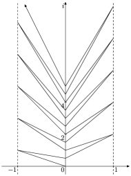
Figure 1: Example 2.1: beginning of curve $\gamma$.

$0$ to $\infty$. We then let $\gamma^{j}=2^{-j}\gamma$: it is easy to see that as $\varepsilon\to 0$, the rescaled curves $\gamma^{j}$ converge, both with respect to $d_{*}^{\mathcal{H}}$ and with respect to $d_{x}^{R}$ for any $x\in\mathbb{H}$ off the imaginary axis, to the simple path that traces the imaginary axis. However, it is clear that the $\gamma^{j}$ have no $d_{\mathcal{U}}$ limit.

Example 2.2.

We consider curves traveling chordally in $\overline{\mathbb{D}}$ between $-1$ and $1$. Let $\eta_{i}\dvtx[0,1]\to\mathbb{C}$ ($1\leq i\leq 3$) be defined by

$$\eta_{1}(t) := -1+(1+i)t,$$

$$\eta_{2}(t) := i-2it,$$

$$\eta_{3}(t) := -i+(1+i)t$$

and let $\gamma=\eta_{1}\eta_{2}\eta_{3}$ [Figure 2(c)]; note that $\gamma\in\Gamma_{\mathrm{t.s.}}$. We can easily find a sequence $(\gamma_{1}^{j})$ in $\Gamma_{\mathrm{sim}}$ converging uniformly to $\gamma$ [Figure 2(a)]. We can likewise find a sequence $(\gamma_{2}^{j})$ in $\Gamma_{\mathrm{sim}}$ converging uniformly to $\tilde{\gamma}:=\eta_{1}\eta_{2}\eta_{2}^{-}\eta_{2}\eta_{3}$ [Figure 2(b)]. But both the $\gamma_{1}^{j}$ and the $\gamma_{2}^{j}$ converge with respect to $d^{R}$ to $\gamma$, and with respect to $d^{L}$ to $\gamma^{-}$. Letting $(\gamma^{j})$ be the sequence obtained by interweaving $(\gamma_{1}^{j})$ and $(\gamma_{2}^{j})$, we have

$$\lim_{j\to\infty}d^{R}(\gamma^{j},\gamma)=\lim_{j\to\infty}d^{L}(\gamma^{j-},\gamma^{-})=0,$$

but clearly $(\gamma^{j})$ is not $d_{\mathcal{U}}$-Cauchy. Figure 3 illustrates essentially the same example

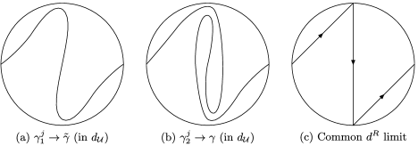
Figure 2: Example 2.2: $d^{R}$ limit with boundary intersections.

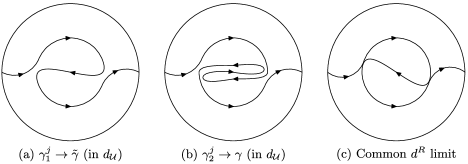
Figure 3: Example 2.2: $d^{R}$ limit with self-intersections.

when the $d^{R}$ and $d^{L}$ limiting curves are allowed to have self-intersections but not boundary intersections.

Example 2.3.

A useful construction for us is the curve $P$ which is formed by taking the straight path from $0$ to $1$ and adding increasingly small, mutually disjoint loops at the dyadic points; these loops are traveled in the clockwise direction. To be more precise, begin with the straight path $P_{0}$ from $0$ to $1$. For each $k\in\mathbb{N}$, let $t_{k,j}=2^{-k+1}j+2^{-k}$ for $0\leq j\leq 2^{k-1}$. Given $P_{k-1}$, for each $j$ define a small clockwise loop $\ell_{k,j}$ which begins and ends at $t_{k,j}$ and otherwise is contained in $\mathbb{H}$; the size of the $\ell_{k,j}$ should tend to zero in $k$. Set $P_{k}$ to be $P_{k-1}$ with the $\ell_{k,j}$ added, so that the time $P_{k-1}$ spends on each $(t_{k,j}-2^{-k},t_{k,j}+2^{-k})$ is divided in thirds between $(t_{k,j}-2^{-k},t_{k,j})$, the loop $\ell_{k,j}$, and $(t_{k,j},t_{k,j}+2^{-k})$. Figure 4 shows the first few iterations of this construction. We will refer to the limiting curve $P$ as the “dyadic loops curve based on $[0,1]$”; it is clear that we can construct a dyadic loops curve based on any simple curve. If a curve first traces $[0,1]$ and then traces backwards the path of diadic loops, then all of the points on $[0,1]$ will be double points, but there will be a dense collection of times mapping to nondouble points.

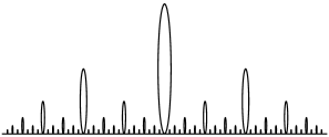
Figure 4: Construction of dyadic loops curve.

Consider the simple curve shown in Figure 5: first it travels the left part of the curve from $-1$ to $-1+3i$, with loops to the left and $U$-shaped “hooks” to the right; each “hook” is a path

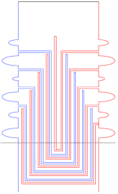
Figure 5: Example 2.3.

that passes below the dotted line, then returns upward to approximately the place it started, then approximately retraces itself. The curve then goes right to $1+3i$ and travels the right part of the curve from $1+3i$ to $1$, with loops to the right and hooks to the left; again, all hooks are bent to pass below the dotted line. The hooks on the two sides are interlocking: thus, for the curve traveled in either direction, each successive hook is mostly “harmonically enclosed” within previous hooks.

We define a sequence of curves $\gamma^{j}\in\Gamma_{\mathrm{sim}}$ which are versions of this curve, so the hooks and loops become more numerous, and the distance between the two vertical sides decreases to zero, as $j\to\infty$. One then sees that for all $x$ in a countable dense set, $\gamma^{j}$ converges with respect to both $d_{x}^{R}$ and $d_{x}^{L}$ to the dyadic loops curve $\gamma$ which travels clockwise around the boundary of the line segment between $0$ and $3i$. But it is clear that the $\gamma^{j}$ do not converge uniformly to $\gamma$.

Before giving Example 2.5, we present here a simplified version:

Example 2.4.

Let $(\gamma_{1}^{j})$ be a sequence of simple curves such as the one shown in Figure 6(a), converging uniformly to the curve $\gamma$ shown in Figure 6(b). Write $\gamma:=\eta_{1}\eta_{2}\eta_{3}\eta_{4}\eta_{5}\eta_{6}$ where the numbering is as in the figure. Now define $\tilde{\gamma}:=\eta_{1}\eta_{2}\eta_{4}\eta_{3}\eta_{5}\eta_{6}$, and let $(\gamma_{2}^{j})$ be a sequence of simple curves converging uniformly to $\tilde{\gamma}$. Let $(\gamma^{j})$ be the sequence obtained by interweaving the $\gamma_{1}^{j}$ and $\gamma_{2}^{j}$. It can be checked that the $\gamma^{j}$ are Cauchy with respect to $d_{x}^{R}$ and $d_{x}^{L}$ for every $x\in\Psi$, but they clearly are

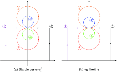
Figure 6: Example 2.4: incompatible forward and reverse limits.

not $d_{\mathcal{U}}$-Cauchy. In this example the $\gamma^{j}$ do not converge with respect to every $x\in\Psi$ to continuously driven curves (i.e., to limits in $\Gamma^{R}$ or $\Gamma^{L}$). For example, if $x$ lies inside the uppermost inner loop $\eta_{4}$, then the $\gamma^{j}$ converge in driving function to the curve $\eta_{1}\eta_{2}\eta_{4}$, which does not lie in $\Gamma^{R}$. (Nevertheless, this curve can be generated by a continuous driving function with respect to $x$.)

Example 2.5.

We now present a modification of Example 2.4 in which all $d_{x}^{R}$ and $d_{x}^{L}$ limits lie in $\Gamma^{R}$ and $\Gamma^{L}$, respectively.

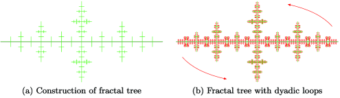
Figure 7: Example 2.4: incompatible forward and reverse limits.

The main construction we will use is the “fractal tree,” the beginning iterations of which are shown in Figure 7(a). We leave it to the reader to verify that this tree can be constructed so that the curve which traces its boundary clockwise (i.e., traces the conformal boundary of the complement of the tree) has a dense set of times mapping to double points and avoids a countable dense subset of $\mathbb{H}$. Moreover, if we then traverse the boundary counterclockwise and add small loops beginning and ending at the same prime end of the conformal boundary [Figure 7(b)], in the limit we will obtain a curve which is continuously driven in the forward but not the reverse direction. We will refer to the counterclockwise portion of the curve as the “dyadic loops curve based on the fractal tree.” From now on, we will use the diagram in Figure 7(b) to indicate this limiting curve.

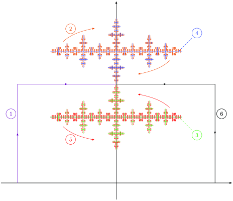
Figure 8: Example 2.5: $d_{\mathcal{U}}$ limit $\gamma$.

Consider now the curve $\gamma$ which is shown in Figure 8. It is the concatenation of $\eta_{i}$ ($1\leq i\leq 6$), where:

1. $\eta_{1}$ is the linear interpolation of the points $-1$, $-1+3i$, $3i$;

2. $\eta_{2}$ is the clockwise dyadic loops curve based on the upper fractal tree;

3. $\eta_{3}$ travels the lower fractal tree clockwise beginning and ending at $3i$;

4. $\eta_{4}$ travels the upper fractal tree counterclockwise beginning and ending at $3i$;

5. $\eta_{5}$ is the counterclockwise dyadic loops curve based on the lower fractal tree;

6. $\eta_{6}$ is the interpolation of the points $3i$, $1+3i$, $1$.

Let $\Psi$ be a countable dense subset of $\mathbb{H}$ avoiding $\gamma$; we leave it to the reader to verify that one exists. We then define $\tilde{\gamma}:=\eta_{1}\eta_{2}\eta_{4}\eta_{3}\eta_{5}\eta_{6}$.

We can find simple curves $\gamma_{1}^{j},\gamma_{2}^{j}$ converging uniformly to $\gamma,\tilde{\gamma}$, respectively; by interweaving the sequences we obtain a sequence $(\gamma^{j})$ which fails to converge uniformly. But we can check that for all $x\in\Psi$, we have $d_{x}^{R}(\gamma^{j},\gamma_{1})\to 0$ where $\gamma_{1}:=\eta_{1}\eta_{2}\eta_{3}\eta_{5}\eta_{6}$, and $d_{x}^{L}(\gamma^{j-},\gamma_{2}^{-})\to 0$ where $\gamma_{2}:=\eta_{1}\eta_{2}\eta_{4}\eta_{5}\eta_{6}$. We have $\gamma_{1}\in\Gamma^{R}$ and $\gamma_{2}\in\Gamma^{L}$, but $\gamma_{2}\neq\gamma_{1}^{-}$ so the forward and reverse limits are incompatible.

3 Driving function convergence

In this section we present (along with a few related facts) a known implication of $d_{x}^{R}$ convergence, namely Carathéodory convergence.

Remark 3.1.

All of the results in this section continue to hold if $\Psi$ is replaced with some $\Psi^{\prime}$ which is the union of $\Psi$ with a countable dense subset of $\overline{\mathbb{R}}\setminus\{-1,1\}$, and the path spaces $\Gamma^{R}$, $\Gamma^{L}$, etc. are redefined accordingly. When $x\in\mathbb{R}$, the metrics $d_{x}^{L}$ and $d_{x}^{R}$ correspond to chordal rather than radial Loewner driving functions.

We let $\Gamma_{\mathrm{init}}^{R}$ denote the space of all curves which can arise as closed initial segments of curves in $\Gamma^{R}$; we define $\Gamma_{\mathrm{init}}^{L}$ similarly. All the definitions of Section 1 (filling processes, distance functions, etc.) can be made for these spaces in exactly the same way. In particular, if $\gamma^{j},\gamma\in\Gamma^{R}$ with $d_{x}^{R}(\gamma^{j},\gamma)\to 0$, then, under the $\operatorname{cap}_{x}$ parametrization, we have $d_{x}^{R}(\gamma^{j}[0,t],\gamma[0,t])\to 0$ as well for any $t$. The distance $d_{x}^{R}$ is a metric on $\Gamma_{\mathrm{init}}^{R}/\sim_{x}$.

Proposition 3.2

For each $x\in\Psi$, the spaces $\Gamma^{R}/\sim_{x}$ and $\Gamma^{L}/\sim_{x}$ are separable with respect to the topology generated by $d_{x}^{R}$ and $d_{x}^{L}$, respectively; likewise $\Gamma^{R}/\sim_{1}$ and $\Gamma^{L}/\sim_{-1}$ are separable with respect to the topology generated by $d^{R}$ and $d^{L}$, respectively. Also, $\Gamma$ is separable with respect to the topology generated by $d_{\mathcal{U}}$.

For the separability of $\Gamma^{R}/\sim_{x}$ it suffices to prove separability of a larger metric space: for metric spaces separability is equivalent to second-countability, and second-countability is inherited in the subspace topology (see, e.g., munkres ).

It is easy to see that the space of all pairs $(W,T)$ where $T>0$ and $W\dvtx\allowbreak[0,T]\to\mathbb{R}$ is continuous, is separable under the metric (4): a countable dense set can be constructed by taking $W$ continuous and linear (with rational derivative) on each of a finite set of rational-length intervals which partition $[0,T]$, for $T$ rational. Separability immediately follows for $\Gamma^{R}/\sim_{x}$ and $\Gamma^{L}/\sim_{x}$, and it follows for $\Gamma^{R}/\sim_{1}$, and $\Gamma^{R}/\sim_{-1}$ by a similar argument. For the metric $d_{\mathcal{U}}$ a countable dense subset of $\Gamma$ can similarly be given using functions which are piecewise linear as maps into $\mathbb{H}$.

3.1 Carathéodory convergence

We begin by recording some preliminary consequences of $d_{x}^{R}$ convergence for a fixed $x\in\Psi$. Extending our previous notation, if $x\in\Psi$ and $\gamma$ in $\Gamma_{\mathrm{init}}^{R}$ or $\Gamma_{\mathrm{init}}^{L}$ is parametrized according to $\operatorname{cap}_{x}$, then $\mathbb{H}_{x,t}=\mathbb{H}_{x,t}(\gamma)$ denotes the unique component of $\mathbb{H}\setminus\gamma[0,t]$ containing $x$, and $K_{x,t}=K_{x,t}(\gamma)=\mathbb{H}\setminus\mathbb{H}_{x,t}$ denotes the filling with respect to $x$ at time $t$. If $T=\operatorname{cap}_{x}\gamma$ then we will generally drop the time subscript and simply write $\mathbb{H}_{x}=\mathbb{H}_{x}(\gamma),K_{x}=K_{x}(\gamma)$. We let $\overline{\mathbb{H}}_{x,t}$ denote the closure of $\mathbb{H}_{x,t}$ in $\overline{\mathbb{H}}$ under the $d_{*}$ metric.

Definition 3.3.

Let $g^{j}=(g_{t}^{j})_{0\leq t\leq T},g=(g_{t})_{0\leq t\leq T}$ be (radial or chordal) Loewner chains with respect to $x$, defined on $\mathbb{H}$. We say that $g^{j}$ converges to $g$ in the Carathéodory sense with respect to $x$, denoted $g^{j}\stackrel{{\scriptstyle\mathit{Cara}}}{{\longrightarrow}}_{x}g$, if for all $\varepsilon>0$ and $t\leq T$, $g^{j}\to g$ uniformly on

$$[0,t]\times\overline{\mathbb{H}}{}^{(\varepsilon)}_{x,t}\qquad\mbox{where }\overline{\mathbb{H}}{}^{(\varepsilon)}_{x,t}:=\{z\in\overline{\mathbb{H}}\dvtx d_{*}(z,\overline{K}_{x,t})\geq\varepsilon\}.$$

In particular, this implies that $g_{t}^{j}\to g_{t}$ pointwise on $\mathbb{H}_{x,t}$ for each $t$. Also, $\operatorname{Im}g_{t}^{j}(z)$ has a nonzero limit as $j\to\infty$ if and only if $z\in\mathbb{H}_{x,t}$.

The following proposition relates driving function convergence to Carathéodory convergence. The result for chordal Loewner chains is proved in lawler ; the proof for radial Loewner chains is entirely similar and we omit it here.

Proposition 3.4

Let $g^{j}=(g_{t}^{j})_{0\leq t\leq T},g=(g_{t})_{0\leq t\leq T}$ be Loewner chains corresponding to the driving functions $W_{t}^{j},W_{t}$, all with respect to $x$. If $W_{t}^{j}\to W_{t}$ uniformly on $[0,T]$, then $g^{j}\stackrel{{\scriptstyle\mathit{Cara}}}{{\longrightarrow}}_{x}g$.

Corollary 3.5

Let $\gamma^{j},\gamma\in\Gamma_{\mathrm{init}}^{R}$ with $T^{j}=\operatorname{cap}_{x}\gamma^{j}$, $T=\operatorname{cap}_{x}\gamma$ and let $g^{j},g$ denote the Loewner chains with respect to $x$ corresponding to $\gamma^{j},\gamma$, respectively. Suppose $d_{x}^{R}(\gamma^{j},\gamma)\to 0$. Then $(g_{s}^{j})_{0\leq s\leq t}\stackrel{{\scriptstyle\mathit{Cara}}}{{\longrightarrow}}_{x}(g_{s})_{0\leq s\leq t}$ for all $t<T$. We also have $g_{T_{j}}^{j}\to g_{T}$ uniformly on $\overline{\mathbb{H}}{}^{(\varepsilon)}_{x}:=\overline{\mathbb{H}}{}^{(\varepsilon)}_{x,T}$.

The first statement follows directly from Proposition 3.4. For the second statement, fix $\delta>0$, and note that if we replace $g^{j},g$ by the Loewner chains $h^{j},h$ corresponding to the driving functions $W_{x,t\wedge T^{j}},W_{x,t\wedge T}$, respectively, then $h_{t}^{j},h_{t}$ are defined for all $t\geq 0$ (with $h_{t}=g_{t}$ for $t\leq T$ and $h_{t}^{j}=g_{t}^{j}$ for $t\leq T^{j}$). By Proposition 3.4, for all $\varepsilon>0$ and for all $t<\infty$, we will have $\|h^{j}-h\|_{\infty}<\delta$ on $[0,t]\times\overline{\mathbb{H}}{}^{(\varepsilon)}_{x,t}$ for $j$ sufficiently large. Also, by uniform continuity of $h$ on $[0,t]\times\overline{\mathbb{H}}{}^{(\varepsilon)}_{x,t}$, we will have $|h_{T^{j}}(z)-h_{T}(z)|<\delta$ for all $z\in\overline{\mathbb{H}}{}^{(\varepsilon)}_{x,T\vee T^{j}}$ for $j$ sufficiently large. Therefore

$$|g_{T^{j}}^{j}(z)-g_{T}(z)|=|h_{T^{j}}^{j}(z)-h_{T}(z)|\leq|h_{T^{j}}^{j}(z)-h_{T^{j}}(z)|+|h_{T^{j}}(z)-h_{T}(z)|<2\delta$$

for all $z\in\overline{\mathbb{H}}{}^{(\varepsilon)}_{x,T\vee T^{j}}$ and $j$ sufficiently large. The result follows by noting that for any $\varepsilon>0$, we can find $\varepsilon^{\prime}>0$ small enough so that $\overline{\mathbb{H}}{}^{(\varepsilon)}_{x,T}\subseteq\overline{\mathbb{H}}{}^{(\varepsilon^{\prime})}_{x,s}$ for $s$ sufficiently close to $T$.

Remark 3.6.

Given a Loewner chain $g\!=\!(g_{t})_{0\leq t\leq T}$ corresponding to $\gamma\!\in\!\allowbreak\Gamma_{\mathrm{init}}^{R}$, for any $s<T$ we can also consider the maps $g^{(s)}=(g_{t}^{(s)})_{0\leq t\leq T-s}$ which satisfy $g_{s+t}=g_{t}^{(s)}\circ g_{s}$. These correspond to the curve $\gamma^{(s)}(t):=g_{s}(\gamma(s+t))$ defined for $0\leq t\leq T-s$, and it is easily seen that $g^{(s)}$ is simply a Loewner chain with driving function $W_{t}^{(s)}:=W_{s+t}$. Thus, if we have $d_{x}^{R}(\gamma^{j},\gamma)\to 0$ as in the corollary above, then also $d_{x}^{R}(\gamma^{j,(s)},\gamma^{(s)})\to 0$ for any $s<T$.

The following corollary will be useful for determining the uniform limit of a sequence of curves from their Carathéodory convergence.

Corollary 3.7

Let $x\in\Psi$, and let $\gamma^{j},\gamma\in\Gamma_{\mathrm{init}}^{R}$ with $d_{x}^{R}(\gamma^{j},\gamma)\to 0$. Then: [(a)]

For any $\varepsilon>0$, $\overline{\mathbb{H}}{}^{(\varepsilon)}_{x}(\gamma)$ is a subset of $\mathbb{H}_{x}(\gamma^{j})$ for sufficiently large $j$.

If $U$ is a connected open subset of $\mathbb{H}$ with $x\in\overline{U}$, and $U\subseteq\mathbb{H}_{x}(\gamma^{j})$ for large $j$, then $U\subseteq\mathbb{H}_{x}(\gamma)$.

If $K_{\dagger}$ is any $d_{*}^{\mathcal{H}}$ subsequential limit of the $K_{x}(\gamma^{j})$, and $\mathbb{H}_{\dagger}$ is the unique component of $\mathbb{H}\setminus K_{\dagger}$ whose closure contains $x$, then $\mathbb{H}_{\dagger}=\mathbb{H}_{x}(\gamma)$.

Let $(g_{x,t})$ and $(g_{x,t}^{j})$ denote the Loewner chains corresponding to $\gamma^{j}$ and $\gamma$, respectively. Throughout this proof we will use the notation $g=g_{x,T}$ and $g^{j}=g_{x,T}^{j}$, where $T=\operatorname{cap}_{x}\gamma$ and $T^{j}=\operatorname{cap}_{x}\gamma^{j}$.

(a) By Corollary 3.5, $g^{j}$ must be defined on $\overline{\mathbb{H}}{}^{(\varepsilon)}_{x}(\gamma)$ for sufficiently large $j$.

(b) Suppose for sake of contradiction that $U\cap K_{x}(\gamma)\neq\varnothing$. By the conditions on $U$, for any $k>0$ we can find $z\in\mathbb{H}_{x}(\gamma)$ such that for some $\delta>0$, $d_{*}(z,K_{x}(\gamma))<\delta$ and $B_{k\delta}(z)\subseteq U$. Then $z\in\mathbb{H}_{x}(\gamma^{j})$ for large $j$, and by Carathéodory convergence, the conformal radius of $\mathbb{H}_{x}(\gamma^{j})$ with respect to $z$ converges to the conformal radius of $\mathbb{H}_{x}(\gamma)$ with respect to $z$. But by the Koebe distortion theorem, the inradius of a domain with respect to an interior point is within a constant factor of its conformal radius: by choosing $k$ large enough we can guarantee that $K_{x}(\gamma^{j})$ will intersect $B_{k\delta}(z)$ for large $j$, which gives the desired contradiction.

(c) By (a) it is clear that $\mathbb{H}_{\dagger}\supseteq\mathbb{H}_{x}(\gamma)$. Conversely, if $U$ is a connected open subset of $\mathbb{H}_{\dagger}$ with $x\in\overline{U}$ and $\overline{U}\subset\mathbb{H}_{\dagger}$, then $\overline{U}\subset\mathbb{H}\setminus K_{x}(\gamma^{j})=\mathbb{H}_{x}(\gamma^{j})$ for large $j$, and so by (b) we have $U\subseteq\mathbb{H}_{x}(\gamma)$. Since $\mathbb{H}_{\dagger}$ is a union of such $\overline{U}$ we find $\mathbb{H}_{\dagger}\subseteq\mathbb{H}_{x}(\gamma)$, hence they are equal.

3.2 Hitting probabilities of Brownian motion

Informally, the above corollary says that $d_{x}^{R}$ convergence gives convergence of the “shape” of the fillings $K_{x}(\gamma^{j})$. To identify the location of the “tip” $\gamma(T)$ on $K_{x}(\gamma)$, we next consider hitting probabilities of Brownian motion (i.e., harmonic measure) for segments of the (conformal) boundary of $\mathbb{H}_{x}(\gamma)$.

For $\gamma\in\Gamma_{\mathrm{init}}^{R}$ with $T=\operatorname{cap}_{x}\gamma$, if $x$ is not swallowed by $\gamma$ then we define the left boundary (with respect to $x$) of $\gamma$ to be the maximal (closed) clockwise segment of the conformal boundary of $\mathbb{H}_{x}(\gamma)$ which begins at $\gamma(T)$ and whose intersection with $\mathbb{R}$ has empty interior; we define the right boundary symmetrically. If $x$ is swallowed by $\gamma$ at some time $\tau_{x}\leq T$, the left boundary is defined to be the set of points (more precisely, prime ends) on the conformal boundary of $\mathbb{H}_{x}(\gamma)$ which lie on the left boundary of $\gamma[0,t]$ for any $t<\tau_{x}$. We let $\alpha_{x}^{z}(\gamma)$ denote the probability that a Brownian motion, started at $z\in\mathbb{H}_{x}(\gamma)$ and stopped upon hitting $\gamma\cup\mathbb{R}$, will hit the left boundary of $\gamma$.

Proposition 3.8

Fix $x\in\Psi$, and let $\gamma^{j},\gamma\in\Gamma_{\mathrm{init}}^{R}$ with $d_{x}^{R}(\gamma^{j},\gamma)\to 0$. Then $\alpha_{x}^{z}(\gamma^{j})\to\alpha_{x}^{z}(\gamma)$.

We begin by proving an easier result. First suppose $x$ is not swallowed by $\gamma$. Fix a “reference point” $P\in\mathbb{R}$ with $P<\inf(\gamma\cap\mathbb{R})$, and consider the event that the Brownian motion started at $z\in\mathbb{H}_{x}(\gamma)$ will hit either the left boundary of $\gamma$ or the segment $[P,\inf(\gamma\cap\mathbb{R})]$. If this occurs we say that the Brownian motion hits to the left of the tip with respect to $P$, and we denote the probability of this event by $\alpha_{x}^{z}(\gamma,P)$.

Lemma 3.9

Fix $x\in\Psi$, and let $\gamma^{j},\gamma\in\Gamma_{\mathrm{init}}^{R}$ with $d_{x}^{R}(\gamma^{j},\gamma)\to 0$ such that $x$ is not swallowed by $\gamma$. Then, for any reference point $P$ as above,

$$\alpha_{x}^{z}(\gamma^{j},P)\to\alpha_{x}^{z}(\gamma,P).$$

By the conformal invariance of Brownian motion we consider the problem in $\mathbb{D}$, with $x=0$, $z\in\mathbb{D}$ and $P\in\partial\mathbb{D}$. Let $g_{t},W_{t}$ denote the (radial) Loewner chain and driving function corresponding to $\gamma$, and similarly $g^{j}_{t},W^{j}_{t}$. We write $g=g_{T}$ and $g^{j}=g^{j}_{T_{j}}$ for the terminal Loewner maps. By the conformal invariance of Brownian motion, $\alpha_{x}^{z}(\gamma,P)$ is exactly the probability that a Brownian motion started at $g(z)$ and stopped upon hitting $\partial\mathbb{D}$ will land on the arc going counterclockwise from $g(P)$ to $W_{T}$. Likewise $\alpha_{x}^{z}(\gamma^{j},P)$ is the probability that a Brownian motion started at $g^{j}(z)$ and stopped upon hitting $\partial\mathbb{D}$ will land on the arc going counterclockwise from $g^{j}(P)$ to $W_{T^{j}}^{j}$. But $W^{j}_{T^{j}}\to W_{T}$ by assumption, and $g^{j}\to g$ pointwise on $\overline{\mathbb{D}}\setminus D_{T}(\gamma)$ by Carathéodory convergence, so the result follows.

Proof of Proposition 3.8 First suppose $x$ is not swallowed by $\gamma$. Write $z_{0}=\inf(\gamma\cap\mathbb{R})$ and $z^{j}_{0}=\inf(\gamma^{j}\cap\mathbb{R})$. We can choose $P<z_{0}$ to make the difference $\alpha^{z}_{x}(\gamma,P)-\alpha^{z}_{x}(\gamma)$ arbitrarily small. On the other hand $\alpha^{z}_{x}(\gamma^{j},P)-\alpha^{z}_{x}(\gamma^{j})$ is the probability that a Brownian motion started at $z$ and stopping upon hitting $\gamma^{j}\cup\mathbb{R}$ will land on the segment $[P,z_{0}^{j}]$. By Corollary 3.7 we must have $\liminf z_{0}^{j}\geq P$. If $\limsup z_{0}^{j}\leq P$ then clearly $\alpha^{z}_{x}(\gamma^{j},P)-\alpha^{z}_{x}(\gamma^{j})\to 0$, so the result follows from Lemma 3.9. Therefore suppose $\limsup z_{0}^{j}>P$, so that the curves $\gamma^{j}$ must come close to $z_{0}$ without touching. Then the hitting probability of $[z_{0},z_{0}^{j}]$ must tend to zero (e.g., using the Beurling estimate), so Lemma 3.9 again gives the result.

It remains to check the case of when $x$ is swallowed by $\gamma$, that is, $\tau_{x}(\gamma)\leq T$. We again work in the unit disc, with $x=0$ and $z\in\mathbb{D}$. Suppose $c=\alpha_{0}(\gamma)$ and $\tilde{c}=\lim_{j}\alpha_{0}(\gamma^{j})$ with $|c-\tilde{c}|>\varepsilon$. We have $\lim_{t\uparrow\tau_{0}}\alpha_{0}(\gamma[0,t])=c$, so for any $\delta>0$ we can choose $t<\tau_{0}$ such that $\tau_{0}-t<\delta$ and $|\alpha_{0}(\gamma[0,t^{\prime}])-c|<\delta$ for all $t^{\prime}\geq t$; by the above result we also have for large $j$ that $\alpha_{0}(\gamma^{j}[0,t])$ is within $\delta$ of $c$ but $\alpha_{0}(\gamma^{j}[0,\tau_{0}])$ is within $\delta$ of $\tilde{c}$. Recalling Remark 3.6, we now consider the systems under the maps $g^{j}_{t}$: the curves $\gamma^{j,(t)}(s):=g^{j}_{t}(\gamma(t+s))$ must travel in such a way that $\alpha_{0}(\gamma^{j,(t)}[0,s])$ changes by more than $\varepsilon-2\delta$ within (capacity) time $\tau_{0}-t<\delta$. Taking $\delta\to 0$ we see that this must contradict the hypothesis that $\gamma$ is the initial segment of a continuously driven curve.

Given $\gamma\in\Gamma_{\mathrm{init}}^{R}$, for any closed subset $S$ of $\gamma\cup\mathbb{R}$ we will let $p^{z}_{x}(S;\gamma)$ denote the probability that Brownian motion started at $z$ and stopped upon hitting $\gamma\cup\mathbb{R}$ will be stopped on $S$ (regardless of whether it stops on the left or right boundary of $\gamma$).

Corollary 3.10

Fix $x\in\Psi$, and let $\gamma^{j},\gamma\in\Gamma_{\mathrm{init}}^{R}$ with $d_{x}^{R}(\gamma^{j},\gamma)\to 0$. Let $T=\operatorname{cap}_{x}\gamma$ and $T^{j}=\operatorname{cap}_{x}\gamma^{j}$. Then, for any $t<T$,

$$\lim_{j\to\infty}p_{x}^{z}(\gamma^{j}[t,T^{j}];\gamma^{j})=p_{x}^{z}(\gamma[t,T];\gamma).$$

It follows that for $s<t<T$, $p_{x}^{z}(\gamma^{j}[s,t];\gamma^{j})\to p_{x}^{z}(\gamma[s,t];\gamma)$.

The first claim follows from Remark 3.6 by applying Proposition 3.8 to the curves $\gamma^{j,(t)}[0,T^{j}-t]$ and $\gamma^{(t)}[0,T-t]$. The second claim is an immediate consequence, since $p^{z}_{x}(\gamma[s,t];\gamma)=p^{z}_{x}(\gamma[s,T];\gamma)-p^{z}_{x}(\gamma[t,T];\gamma)$.

For our purposes it will suffice to consider only $p_{x}^{x}(\cdot;\cdot)$, which we will denote from now on by $p_{x}(\cdot;\cdot)$. [Note, however, that when $\Psi$ is replaced by $\mathbb{Q}$ or $\{\pm 1\}$ it will still be useful to consider $p_{x}^{z}(\cdot;\cdot)$ for general $z\in\mathbb{H}_{x}(\gamma)$.]

4 Convergence of deterministic curves

In this section we will prove Theorem 1.2.

4.1 Hausdorff convergence and compatibility

Lemma 4.1

Let $\gamma^{j},\gamma\in\Gamma_{\mathrm{init}}^{R}$ with $d_{x}^{R}(\gamma^{j},\gamma)\to 0$ for all $x\in\Psi$. Then $d_{*}^{\mathcal{H}}(\gamma^{j},\gamma)\to 0$.

For any $\varepsilon>0$ it is possible to choose finitely many points $x_{1},\ldots,x_{n}\in\Psi$ such that $Q:=\bigcup_{i=1}^{n}\overline{\mathbb{H}}{}^{(\varepsilon)}_{x}(\gamma)$ contains every point $z\in\overline{\mathbb{H}}$ with $d_{*}(z,\gamma)\geq\varepsilon$. Applying Corollary 3.7(a) to each component separately shows that $\gamma^{j}\cap Q=\varnothing$ for sufficiently large $j$, hence $\gamma^{j}$ is contained in an $\varepsilon$-neighborhood of $\gamma$ for sufficiently large $j$.

For the other direction, let $y\in\gamma$, and let $U=B_{\varepsilon}(y)$. Then $d_{x}^{R}(\gamma^{j},\gamma)\to 0$ for some $x\in U\cap\Psi$, and so by Corollary 3.7(b) it must be that $U$ intersects $\gamma^{j}$ for large $j$. Since $\gamma$ is compact, it follows that it will be contained in an $\varepsilon$-neighborhood of $\gamma^{j}$ for large $j$, which concludes the proof.

The next lemma tells us that even if we are not given a single curve to which the $\gamma^{j}$ converge in all the $d_{x}^{R}$ metrics, we can almost construct it from knowing the $d_{x}^{R}$ limits for each $x\in\Psi$:

Lemma 4.2

Let $(\gamma^{j})$ be a sequence in $\Gamma_{\mathrm{init}}^{R}$, and suppose that for each $x\in\Psi$ there exists $\gamma^{x}\in\Gamma^{R}$ with $d_{x}^{R}(\gamma^{j},\gamma^{x})\to 0$. Then there exists a unique half-open path $\eta\dvtx[0,1)\to\overline{\mathbb{H}}$ such that each $\hat{\gamma}^{x}:=\gamma^{x}[0,\tau_{x}(\gamma^{x})]$ is an initial segment of $\eta$ and $\eta=\bigcup_{x}\hat{\gamma}^{x}$ (up to the inclusion of endpoints).

Let $x_{1},x_{2}$ be two distinct points in $\Psi$. For $i=1,2$ we let $\gamma^{x_{i}}$ be parametrized by $\operatorname{cap}_{1}$, and set

$$\tau^{i}_{j}=\inf\{t\geq 0\dvtx x_{j}\notin\mathbb{H}_{t}(\gamma^{x_{i}})\}.$$

Set $\sigma^{i}=\tau^{i}_{1}\wedge\tau^{i}_{2}$; this is the first time $t$ such that either the $x_{i}$ lie in different components of $\mathbb{H}\setminus\gamma^{x_{i}}[0,t]$, or that they both no longer lie in $\mathbb{H}_{t}(\gamma^{x_{i}})$, the unique component of $\mathbb{H}\setminus\gamma^{x_{i}}[0,t]$ whose closure contains $1$. Then set $\sigma=\sigma^{1}\wedge\sigma^{2}$; we claim that the $\gamma^{x_{i}}$ must agree up to time $\sigma$. To see this, let $t<\sigma$: by definition of $\sigma$ we must have $\mathbb{H}_{t}(\gamma^{x_{i}})=\mathbb{H}_{x_{1},t}(\gamma^{x_{i}})=\mathbb{H}_{x_{2},t}(\gamma^{x_{i}})$ for $i=1,2$. Let $U$ be a connected open subset of $\mathbb{H}$ with $\overline{U}\subset\mathbb{H}_{x_{1},t}(\gamma^{x_{1}})$ and $x_{1},x_{2}\in U$. Then by Corollary 3.7(a) we have for large $j$ that $U\subset\mathbb{H}_{x_{1},t}(\gamma^{j})$ and $U\subset\mathbb{H}_{x_{2},t}(\gamma^{j})$, hence $\mathbb{H}_{x_{1},t}(\gamma^{j})=\mathbb{H}_{x_{2},t}(\gamma^{j})$. By Corollary 3.7(b) we have $U\subseteq\mathbb{H}_{x_{2},t}(\gamma^{x_{2}})$, and $\mathbb{H}_{x_{1},t}(\gamma^{x_{1}})$ is a union of sets of the form $U$ which proves $\mathbb{H}_{x_{1},t}(\gamma^{x_{1}})\subseteq\mathbb{H}_{x_{2},t}(\gamma^{x_{2}})$, and so by symmetry they are equal. Since the curves are uniquely determined by their filling processes, the $\gamma^{x_{i}}$ must agree up to time $\sigma=\sigma^{1}=\sigma^{2}$.

It follows that one of the $\hat{\gamma}^{x_{i}}$ is an initial segment of the other: $\sigma=\tau^{1}_{j}=\tau^{2}_{j}$ for some $j$, and then the curve $\hat{\gamma}^{x_{j}}$ must end at time $\sigma$. Therefore we can let $\eta$ be the union of all $\hat{\gamma}^{x}$ for $x\in\Psi$; if there is one $\hat{\gamma}^{x}$ of which all other $\hat{\gamma}^{x^{\prime}}$ are initial segments, then $\eta=\hat{\gamma}^{x}$ is a curve going from $-1$ to $1$. If not, we view $\eta$ as a half-open path that does not contain its terminal endpoint.

If $\eta$ is a half-open curve as constructed in Lemma 4.2, we will write $d_{x}^{R}(\gamma^{j},\eta)\to 0$ if $d_{x}^{R}(\gamma^{j},\eta^{\prime})\to 0$ for some (all) $\eta^{\prime}\in\Gamma^{R}$ with $\eta^{\prime}[0,\tau_{x}(\eta^{\prime})]=\hat{\eta}^{x}$. The following is an example showing that this $\eta$ need not extend to a closed continuous curve which contains its terminal endpoint:

Example 4.3.

We consider curves traveling between $0$ and $\infty$ within the closure of the infinite half-strip $D=\{|{\operatorname{Re}z}|<1\}\cap\mathbb{H}$, with the countable dense subset $\Psi=(\mathbb{Q}\cap D)\setminus(i\mathbb{R})$. We will adapt the curve of Example 2.1 as follows: for $n\in\mathbb{N}$, let $z_{n}=(-1)^{n}+in$ as before, but now let $w_{n}=i(1-2^{-n})$. We will let $\eta_{k}$ denote the closed curve which is a linear interpolation of the points

$$0,z_{1},w_{1},\ldots,z_{k-1},w_{k-1},z_{k}.$$

See Figure 9(a) and (b). If we let $\eta$ denote the union over all

Figure 9: Example 4.3: $\eta$ does not extend continuously to closed curve.

$\eta_{k}$, then $\eta$ travels below the line $\{\operatorname{Im}z=1\}$ infinitely many times, and so it does not extend to a continuous closed curve from $0$ to $\infty$. Nevertheless it is easy to find a sequence $(\gamma^{j})$ in $\Gamma_{\mathrm{sim}}$ such that $d_{x}^{R}(\gamma^{j},\eta)\to 0$ for all $x\in\Psi$.

In the next section we will describe how to use bidirectional driving convergence to obtain the desired continuous extension.

4.2 Uniform convergence from bidirectional driving convergence

We begin by proving some useful consequences of the time-separated assumption. From now on we assume that $(\gamma^{j})$ is a sequence in $\Gamma_{\mathrm{sim}}^{R}$. Since these curves extend continuously to their endpoint, if we use the $\operatorname{cap}_{1}$ parametrization we will write $\gamma^{j}[t,\infty]$ for the closure of $\gamma^{j}[t,\infty)$.

Definition 4.4.

Let $\eta$ be a half-open curve such as constructed by Lemma 4.2, parametrized by $\operatorname{cap}_{1}$. We say that a time $t_{0}$ is nondouble if $y_{0}:=\eta(t_{0})$ is a nondouble point of $\eta$. We say that $t_{0}$ is strongly nondouble if in addition $y_{0}$ does not lie in the closure of $\eta[t,\infty)$ for any $t>t_{0}$. We make the symmetric definitions for $\xi$ parametrized by $\operatorname{cap}_{-1}$.

Lemma 4.5

Let $(\gamma^{j})$ be a sequence in $\Gamma_{\mathrm{sim}}$, and suppose that for each $x\in\Psi$ there exists $\gamma^{x}\in\Gamma_{\mathrm{t.s.}}^{R}$ with $d_{x}^{R}(\gamma^{j},\gamma^{x})\to 0$. Then the half-open curve $\eta$ constructed by Lemma 4.2 has a dense collection of nondouble times (under the $\operatorname{cap}_{1}$ parametrization).

For $0<t_{1}<t_{2}<t_{3}$, we say that $z$ is a $(t_{1},t_{2},t_{3})$-double point if $\eta(s)=\eta(s^{\prime})=z$ for some $s\in[0,t_{1}]$, $s^{\prime}\in[t_{2},t_{3}]$. Let $\mathcal{D}_{t_{1},t_{2},t_{3}}$ denote the set of times mapping to $(t_{1},t_{2},t_{3})$-double points. Then $\mathcal{D}_{t_{1},t_{2},t_{3}}$ is a closed subset of $\mathbb{R}_{\geq 0}$, and since $\eta[0,t_{3}]$ is time-separated, it must be that $\mathcal{D}_{t_{1},t_{2},t_{3}}$ has dense complement in $\mathbb{R}_{\geq 0}$: if $\mathcal{D}_{t_{1},t_{2},t_{3}}$ contained a nontrivial time interval, the interval would map to a nontrivial connected component of $\eta[0,t_{1}]\cap\eta[t_{2},t_{3}]$ since $\eta$ is assumed to be continuously driven (hence not locally constant).

The set $\mathcal{D}$ of all times mapping to double points can be expressed as the union of $\mathcal{D}_{t_{1},t_{2},t_{3}}$ over all rational triples $0<t_{1}<t_{2}<t_{3}$. The countable intersection of open dense sets is dense by the Baire category theorem, so $\mathcal{D}$ has dense complement as desired.

We now assume the notation and hypotheses of Theorem 1.2, and let $\eta:=\bigcup_{x}\hat{\eta}^{x}$ and $\xi:=\bigcup_{x}\hat{\xi}^{x}$ be the half-open curves given by Lemma 4.2. At this point we have not yet shown that either curve extends continuously to its terminal endpoint or that one curve is the time reversal of the other. However, we know that if there exists an $x\in\Psi$ that is not swallowed by $\eta$ before its terminal time, then $\eta=\hat{\eta}^{x}$ and hence $\eta$ extends continuously to its endpoint. We also know that $\mathbb{H}_{x}(\eta)=\mathbb{H}_{x}(\eta^{x})=\mathbb{H}_{x}(\xi^{x})=\mathbb{H}_{x}(\xi)$ for every $x\in\Psi$, since these sets are components of the complement of the Hausdorff limit of the $\gamma^{j}$ (see Lemma 4.1). Thus, as sets, both $\eta$ and $\xi$ contain

$$\bigcup_{x\in\Psi}\overline{\partial\mathbb{H}_{x,\infty}(\eta)\setminus\mathbb{R}},$$

and both are contained in the closure of this union.

Lemma 4.6

Let $\eta$ and $\xi$ be defined as above, parametrized by $\operatorname{cap}_{1}$ and $\operatorname{cap}_{-1}$, respectively. Under this parametrization, each curve has a dense collection of strongly nondouble times.

Suppose for the sake of contradiction that there is a time interval $[t_{1},t_{2}]$ (with $t_{1}<t_{2}$) in which every time fails to be a strongly nondouble time for $\eta$. By Lemma 4.5, this time interval does contain a dense set of nondouble times $t_{0}$, so it must be that each corresponding $y_{0}:=\eta(t_{0})$ arises as the subsequential limit of $\eta(t)$ for large $t$. Therefore $S:=\eta[t_{1},t_{2}]$ must lie in the closure of $\eta[t,\infty)$ for any $t>t_{2}$. We claim that for such $t$, any subsequential $d_{*}^{\mathcal{H}}$ limit of the sets $\gamma^{j}[t,\infty]$ must contain $S$. Indeed, by Lemma 4.1 the limit must contain $\eta[t,\infty)\setminus\eta[0,t]$. Since $\eta$ is continuously driven, $\eta[t,\infty)\setminus\eta[0,t]$ is dense in $\eta[t,\infty)$. Since any $d_{*}^{\mathcal{H}}$ limit is closed, this proves the claim.

It is clear that we can assume that $t_{2}$ is a nondouble time. We therefore consider the following two cases:

Case 1. Suppose that after time $t_{2}$, $\eta$ first hits $(\eta[0,t_{2}]\cup\mathbb{R})\setminus\{\eta(t_{2})\}$ at some time $t_{3}>t_{2}$. Let $x\in\Psi$ be such that $x$ is swallowed at this time, and such that some nontrivial connected subset $S^{\prime}$ of $\partial S$ is contained in the boundary of $U_{x}:=\mathbb{H}_{x}(\eta)$. (That such $x$ exists is easy to see from the definition of $t_{3}$, for example, by a simple compactness argument.) By re-labeling we now suppose that the times $t_{i}$ ($1\leq i\leq 3$) are all with respect to the $\operatorname{cap}_{x}$ parametrization.

Now, in the reverse direction, let $\acute{t}_{i}^{j}$ ($1\leq i\leq 3$) be defined by $\gamma^{j}(t_{i})=\gamma^{j-}(\acute{t}_{i}^{j})$ (again, with respect to $\operatorname{cap}_{x}$). By passing to a subsequence we may suppose that $\acute{t}_{i}^{j}$ converges to some $\acute{t}_{i}$ for each $i$. By hypothesis, $\gamma^{j-}[0,\acute{t}_{3}^{j}]$ converges to $\xi[0,\acute{t}_{3}]$ with respect to $d_{x}^{L}$ for all $x\in\Psi$, and by Lemma 4.1 it converges in $d_{*}^{\mathcal{H}}$ as well, so by the first claim above $\xi[0,\acute{t}_{3}]\supseteq S$. Since $\xi$ is time-separated, during the time interval $[\acute{t}_{3},\acute{t}_{1}]$ it can only hit a (closed) totally disconnected subset of $S$. Therefore, we can find a point $y$ in the interior of $S^{\prime}$ (in the subspace topology on $S^{\prime}$) such that a small neighborhood $V$ of $y$ is not hit by $\xi[\acute{t}_{3},\acute{t}_{1}]$. We can then choose $z\in U_{x}$ close enough to $y$ such that with probability at least $1-\varepsilon$ (for small $\varepsilon>0$), a Brownian motion started at $z$ and stopped upon hitting $\partial U_{x}$ will stop on $V\cap S^{\prime}$, so that $p^{z}_{x}(\xi[\acute{t}_{2},\acute{t}_{1}];\xi)\leq\varepsilon$. But on the other hand $S^{\prime}\subseteq\eta[t_{1},t_{2}]$, so $p^{z}_{x}(\eta[t_{1},t_{2}];\eta)\geq 1-\varepsilon$. The contradiction follows from noting that by Corollary 3.10,

$$p^{z}_{x}(\eta[t_{1},t_{2}];\eta) = \lim_{j\to\infty}p^{z}_{x}(\gamma^{j}[t_{1},t_{2}];\gamma^{j})=\lim_{j\to\infty}p^{z}_{x}(\gamma^{j-}[\acute{t}_{2}^{j},\acute{t}_{1}^{j}];\gamma^{j-})$$

$$= p^{z}_{x}(\xi[\acute{t}_{2},\acute{t}_{1}];\xi).$$

Case 2. Now suppose $\eta$ never hits $(\eta[0,t_{2}]\cup\mathbb{R})\setminus\{\eta(t_{2})\}$ after time $t_{2}$, and let $z$ be any point of $\Psi$ that is swallowed by $\eta$ after time $t_{2}$, say at time $t_{3}$. Note that $\eta(t_{2})$ forms a cut point of $\eta[0,t_{3}]$. Now, $\eta$ must swallow every point of $\Psi$ eventually: if some $x\in\Psi$ does not get swallowed then we would have $\eta^{x}=\eta$, but by hypothesis the $\eta^{x}$ lie in $\Gamma_{\mathrm{t.s.}}$, and hence extend continuously to their endpoints, while $\eta$ does not. Consider those points $x\in\Psi$ which lie in a neighborhood of the cut point $\eta(t_{2})$ and which have not been swallowed by time $t_{2}$: since all of these points must eventually be swallowed (but they cannot all be swallowed at once since $\eta$ never hits $(\eta[0,t_{2}]\cup\mathbb{R})\setminus\{\eta(t_{2})\}$), we see that the closure of $\eta[t_{3},\infty)$ must surround $z$, and thus the $d_{*}^{\mathcal{H}}$ limits of both $\gamma^{j}[t_{2},t_{3}]$ and $\gamma^{j}[t_{3},\infty]$, which we denote $B$ and $B^{\prime}$, must surround $z$. $B$ and $B^{\prime}$ are connected sets, and neither is contained in the other since $\eta$ and $\xi$ are continuously driven, but by construction $B$ will be “nested” inside $B^{\prime}$. This contradicts the assumption that the $\gamma^{j-}$ converge with respect to $d_{z}^{R}$ to a continuously driven curve.

Note that it follows immediately that there is a dense collection of strongly nondouble times mapping to points not in $\mathbb{R}$, since for continuously driven curves the set of times mapping into $\mathbb{R}$ is closed and totally disconnected.

Lemma 4.7

Assume the notation and hypotheses of Theorem 1.2, and let $\eta:=\bigcup_{x}\hat{\eta}^{x}$ and $\xi:=\bigcup_{x}\hat{\xi}^{x}$ be the half-open curves given by Lemma 4.2, parametrized by $\operatorname{cap}_{1}$ and $\operatorname{cap}_{-1}$, respectively. Let $z_{0}=\eta(t_{0})$ be a strongly nondouble point of $\eta$ with $z_{0}\notin\mathbb{R}$. Fix $t_{*}>t_{0}$, and let $\eta^{j}_{*}$ denote the curve $\gamma^{j}$ stopped at time $t_{*}$. Let $\bar{\eta}^{j}_{*}$ denote the remaining curve $\gamma^{j}\setminus\eta^{j}_{*}$. Then, if $X$ is any (subsequential) $d_{*}^{\mathcal{H}}$ limit of the $\bar{\eta}^{j}_{*}$, we will have $z_{0}\notin X$.

Since $z_{0}$ is a strongly nondouble point, we can find $\varepsilon>0$ small enough so that $\eta$ does not enter $\overline{B_{\varepsilon}(z_{0})}$ after time $t_{*}$. We further require $B_{\varepsilon}(z_{0})\subset\mathbb{H}$. By the Beurling estimate, for any $\delta>0$ we may choose $0<\varepsilon^{\prime}<\varepsilon$ small enough so that for any curve $P$ crossing the annulus $\{\varepsilon^{\prime}<|z-z_{0}|<\varepsilon\}$, a Brownian motion started inside $B_{\varepsilon^{\prime}}(z_{0})$ has probability less than $\delta$ of exiting $B_{\varepsilon}(z_{0})$ without hitting $P$. Thus for $x\in B_{\varepsilon^{\prime}}(z_{0})\cap\Psi$ we will have $p_{x}(\eta[t_{*},\infty);\eta)<\delta$ and $p_{x}(\mathbb{R};\eta)<\delta$, and so by Corollary 3.10

$$\lim_{j\to\infty}p_{x}(\bar{\eta}^{j}_{*};\gamma^{j})<\delta\quad\mbox{and}\quad\lim_{j\to\infty}p_{x}(\mathbb{R};\gamma^{j})<\delta.$$ (5)

We now consider the reverse direction. Let $0<\varepsilon^{\prime\prime}<\varepsilon^{\prime}$ and

$$s_{1}:=\inf\{t\geq 0\dvtx\xi(t)\in B_{\varepsilon^{\prime\prime}}(z_{0})\},$$

and note that since $\gamma^{j-}[0,s_{1}]$ has $d_{*}^{\mathcal{H}}$ limit $\xi[0,s_{1}]$ not containing $z_{0}$, a fortiori we have $\gamma^{j-}[0,s_{1}]\subset\bar{\eta}^{j}_{*}$ for large $j$. Now, making use of Lemma 4.6, let $s_{0}<s_{1}$ be a strongly nondouble time of $\xi$ such that $\acute{z}_{0}=\xi(s_{0})$ lies in $\{\varepsilon^{\prime\prime}<|z-z_{0}|<\varepsilon^{\prime}\}$, and let $\tilde{\varepsilon}>0$ be small enough so that $\xi$ does not enter $B_{\tilde{\varepsilon}}(\acute{z}_{0})$ after time $s_{1}$. Applying the Beurling estimate again we choose $0<\tilde{\varepsilon}^{\prime}<\tilde{\varepsilon}$ small enough so that for any curve $P$ crossing $\{\tilde{\varepsilon}^{\prime}<|z-\acute{z}_{0}|<\tilde{\varepsilon}\}$, a Brownian motion started inside $B_{\tilde{\varepsilon}^{\prime}}(\acute{z}_{0})$ has probability less than $\delta$ of exiting $B_{\tilde{\varepsilon}}(\acute{z}_{0})$ without hitting $P$. Then for $x\in B_{\tilde{\varepsilon}}(\acute{z}_{0})\cap\Psi$ we have $p_{x}(\xi[s_{1},\infty);\xi)<\delta$, and so by our observation above

$$\lim_{j\to\infty}p_{x}(\eta^{j}_{*};\gamma^{j})\leq\lim_{j\to\infty}p_{x}(\gamma^{j-}[s_{1},\infty];\gamma^{j-})<\delta.$$ (6)

Combining (5) and (6) gives

$$\lim_{j\to\infty}[p_{x}(\eta^{j}_{*};\gamma^{j})+p_{x}(\bar{\eta}^{j}_{*};\gamma^{j})+p_{x}(\mathbb{R};\gamma^{j})]<3\delta$$

and setting $\delta\leq 1/3$ we obtain a contradiction, since a Brownian motion started at $x$ and stopped upon hitting $\eta\cup\mathbb{R}$ must clearly be stopped at one of $\eta^{j}_{*}$, $\bar{\eta}^{j}_{*}$ or $\mathbb{R}$.

Corollary 4.8

Assume the notation and hypotheses of Theorem 1.2 and Lemma 4.7. The paths $\eta,\xi$ extend continuously to their endpoints and $\eta=\xi^{-}=:\gamma$.

First, notice that if $z_{1},z_{2}$ are strongly nondouble points of $\eta$ not in $\mathbb{R}$ such that $\eta$ hits $z_{1}$ before $z_{2}$, then $\xi$ hits both these points, and will hit $z_{2}$ before $z_{1}$. Indeed, writing $t_{i}=\eta^{-1}(z_{i})$, let $t_{*}\in(t_{1},t_{2})$: by Lemma 4.7, any subsequential $d_{*}^{\mathcal{H}}$ limit $X$ of the curves $\bar{\eta}_{*}^{j}=\gamma^{j}[t_{*},\infty]$ will be a closed initial segment of $\xi$ containing $\eta\setminus\eta[0,t_{*}]$ (hence the point $z_{2}$) but not $z_{1}$.

Suppose now that $\eta(t)$ has multiple limit points as $t\to\infty$, that is, that there exist sequences $t_{i,k}$ (for $i=1,2$) such that $z_{i}=\lim_{k}\eta(t_{i,k})$ with $z_{1}\neq z_{2}$. We may assume that all the $t_{i,k}$ map to strongly nondouble points of $\eta$ not in $\mathbb{R}$, by the continuity of $\eta$ and the density of such times. But then we claim that for any $\varepsilon>0$ the curve $\xi$ must travel between $B_{\varepsilon}(z_{1})$ and $B_{\varepsilon}(z_{2})$ infinitely many times before time $s$ for some $s>0$, which contradicts the continuity of $\xi$. Therefore $\eta$ extends continuously to its endpoint, and it follows from the above that $\eta=\xi$ as sets.

It remains to show that $\xi=\eta^{-}$. We know that there is a dense set of times $t_{k}$ which map to strongly nondouble points of $\eta$ not in $\mathbb{R}$, and that $\xi$ hits these points in reverse order. Under the $\operatorname{cap}_{-1}$ parametrization of $\xi$, let $\mathcal{T}=\{t\dvtx\xi(t)=\eta(t_{k})\mbox{ for some }k\}$. If $\mathcal{T}$ is a dense set of times for $\xi$ then we are done, so suppose that there is an interval of time $I$ not contained in $\overline{\mathcal{T}}$. But $\xi(\overline{\mathcal{T}})=\eta[0,\infty)=\xi[0,\infty)$, and so $I$ is an interval of times mapping to double points, which gives the contradiction. Proof of Theorem 1.2 Let $\eta:=\bigcup_{x}\hat{\eta}^{x}$ and $\xi:=\bigcup_{x}\hat{\xi}^{x}$ be the half-open curves given by Lemma 4.2. Thanks to Corollary 4.8 we finally know that the (strongly) nondouble points of $\eta$ and $\xi$ are the same, as $\gamma=\eta=\xi^{-}$. Let $z_{1}=\gamma(t_{1}),z_{2}=\gamma(t_{2})$ be nondouble points of $\gamma$ with $t_{1}<t_{2}$, and let $\gamma[z_{1},z_{2}]$ denote the portion of $\gamma$ between these two hitting points, viewed as a closed set. We then let $\gamma^{j}[z_{1},z_{2}]$ denote the portion of $\gamma^{j}$ between its nearest approach to $z_{1}$ and its nearest approach to $z_{2}$. (If there is a tie, we choose the earliest one, say.) To show uniform convergence, it suffices to prove that for any such $z_{1}$ and $z_{2}$, we have $\gamma^{j}[z_{1},z_{2}]$ converging along subsequences in the $d_{*}^{\mathcal{H}}$ metric to subsets of $\gamma[z_{1},z_{2}]$.

Let $X$ denote any subsequential $d_{*}^{\mathcal{H}}$ limit of the $\gamma^{j}[z_{1},z_{2}]$, and let $z_{0}=\gamma(t_{0})\notin\mathbb{R}$ be a nondouble point of $\gamma$ with $t_{0}\notin[t_{1},t_{2}]$. We claim that $z_{0}\notin X$: without loss of generality we assume $t_{0}>t_{2}$; then, by Lemma 4.7 applied to the reverse path $\gamma^{-}$, it suffices to show that for some $t\in(t_{2},t_{0})$, the $\gamma^{j}[z_{1},z_{2}]$ are stopped before time $t$ for sufficiently large $j$. But if such a $t$ does not exist, it means that for any $t\in(t_{2},t_{0})$, as $j\to\infty$, we can find subsequences along which the nearest approach of $\gamma^{j}$ to $z_{2}$ occurs after time $t$. But since $z_{2}$ is in the $d_{*}^{\mathcal{H}}$ limit of $\gamma^{j}[0,t_{2}]$, this shows that it will be in the $d_{*}^{\mathcal{H}}$ limit of $\gamma^{j}[t,\infty]$ as well, which is a violation of Lemma 4.7 applied to the forward path $\gamma$.

It follows that $X$ is a connected subset of $\gamma$ contained in

$$C=\gamma[0,t_{2}]\cap\gamma[t_{1},\infty)=\gamma[t_{1},t_{2}]\cup\bigl{(}\gamma[0,t_{1}]\cap\gamma[t_{2},\infty)\bigr{)}\cup(\gamma\cap\mathbb{R}).$$

Since $\gamma$ is continuously driven and time-separated, $\gamma[0,t_{1}]\cap\gamma[t_{2},\infty)$ and $\gamma\cap\mathbb{R}$ are both totally disconnected closed sets, hence their union is as well. Any point of $C$ not contained in $\gamma[t_{1},t_{2}]$ therefore forms a trivial connected component of $C$, so we must have $X\subseteq\gamma[t_{1},t_{2}]$, and the statement of the theorem follows. Proof of Proposition 1.4 This result is essentially a restatement of the remarks following the list of examples in Section 1.4: if $\gamma$ is a simple curve, then $d^{R}(\gamma^{j},\gamma)\to 0$ and $d^{L}(\gamma^{j-},\gamma^{-})\to 0$ together suffice to guarantee $d_{x}^{R}$ and $d_{x}^{L}$ convergence with respect to all $x$ in a dense subset of $\overline{\mathbb{H}}$.

4.3 Alternate proof of uniform convergence

In this section we sketch an alternative proof of Theorem 1.2 that does not use the lemmas of the previous section. Instead of showing the existence of nondouble and strongly nondouble times—and considering segments of the path between these times—we begin by constructing a parametrization of $\eta$ and $\xi$ that behaves well under time-reversal.

Suppose first that $\eta$ is parametrized by capacity time $t$. For any $x\in\Psi$, observe that $f_{x}:=g_{x,\infty}^{-1}\circ\varphi^{-1}$ is a conformal map from the unit disc $\mathbb{D}$ to $\mathbb{H}_{x}(\eta)$ that extends continuously to $\overline{\mathbb{D}}$. Thus, for any $t$,

$$A_{x}(t)\equiv A^{\eta}_{x}(t)=\{\theta\in[0,1]\dvtx f_{x}(e^{2\pi i\theta})\in\eta[0,t]\cap\mathbb{H}\}$$

is a closed subset of $[0,1]$. Let $s_{x}(t)\equiv s^{\eta}_{x}(t)$ be the (Lebesgue) measure of the interior of $A_{x}(t)$, divided by the measure of $A_{x}(\infty)$. Using topological arguments, it is not hard to see that this interior contains at most one interval of $[0,1]$ (viewed topologically as a circle, by identifying endpoints). Thus $s_{x}(t)$ is proportional to the length of this interval. Informally, $s_{x}(t)$ represents the portion (in terms of harmonic measure from $x$) of $\partial\mathbb{H}_{x}(\eta)\setminus\mathbb{R}$ that has been traced by time $t$. Because $\eta$ is continuous, $s_{x}(t)$ is a continuously increasing function of $t$.

Now fix a map $a\dvtx\Psi\to(0,\infty)$ with $\sum_{x\in\Psi}a(x)=1$ and write $s(t)=\break\sum_{x\in\Psi}a(x)s_{x}(t)$. We claim that $s$ is strictly increasing function of $t$. This follows from the time-separation assumption and arguments in the proof of Lemma 4.6, which show that an open dense subset of $\partial(\mathbb{H}\setminus\eta[0,t])\setminus\mathbb{R}$ will remain on the boundary of $\partial(\mathbb{H}\setminus\eta[0,\infty))\setminus\mathbb{R}$.

We therefore take $s\in[0,1)$ to be our new parametrization of $\eta$, and we can assume that $\xi$ is analogously parametrized by $[0,1)$. The proof now proceeds with the following observations:

1. If $t^{j}$ is any sequence of times then the sets $\gamma^{j}[0,t^{j}]$ and $\gamma^{j}[t^{j},\infty]$ must converge (subsequentially) in $d_{*}^{\mathcal{H}}$ to $\eta[0,s]$ and $\xi[0,1-s]$ for some $s$. Indeed, using Lemma 4.1 we already have Hausdorff convergence to some $\eta[0,s]$ and $\xi[0,s^{\prime}]$, and need only check that $s^{\prime}=1-s$. This involves checking for each $x$ that the Hausdorff limits of $\gamma^{j}[0,t^{j}]$ and $\gamma^{j}[t^{j},\infty]$ cannot contain overlapping intervals of $\partial\mathbb{H}_{x}(\eta)$, even though the union of these two limits and $\mathbb{R}$ includes all of $\partial\mathbb{H}_{x}(\eta)$. This is done with the same arguments as those used in the previous section: if the intervals overlapped, then either $\gamma^{j}$ or its time reversal would fail to converge with respect to $x$ to a continuously driven limit.

2. The curve $\eta$ extends continuously to $[0,1]\dvtx\lim_{s\to 1}d_{*}^{\mathcal{H}}(\xi[0,1-s],\{1\})=0$, but $\xi[0,1-s]$ is the Hausdorff limit of $\gamma^{j}[t_{j},1]$ (for some sequence $t_{j}$), and by the above this must contain $\eta\setminus\eta[0,s)$, a dense subset of $\eta[s,1]$. Since $\xi[0,1-s]$ is closed it must contain $\eta[s,1]$ which gives the claim.

3. The above imply that $\eta(s)=\xi(1-s)$ for all $s\in[0,1]$.

4. For any pair of sequences of times $t^{j}_{1}$ and $t^{j}_{2}$ such that $\gamma^{j}[0,t^{j}_{1}]$ tends to $\eta[0,a]$ and $\gamma^{j}[t^{j}_{2},1]$ tends to $\eta[b,1]$, we have Hausdorff convergence of $\gamma^{j}[t^{j}_{1},t^{j}_{2}]$ to a closed subset of $\eta[0,a]\cap\eta[b,1]$, which by time-separation must be simply $\eta[a,b]$.

The latter item implies convergence in $d_{\mathcal{U}}$.

5 Extension to random curves

Now we use Proposition 3.2 and Theorem 1.2 to prove Theorem 1.5: Proof of Theorem 1.5 Each $\gamma^{j}$ can be viewed as a random variable taking values in

$$\Omega_{\Psi}=\prod_{x\in\Psi}\Gamma_{x}^{R}\times\Gamma_{x}^{L},$$

where $\Gamma_{x}^{R}$ is the Polish (complete separable metric) space defined by the completion of $\Gamma^{R}/\sim_{x}$ with respect to $d_{x}^{R}$, and similarly $\Gamma_{x}^{L}$.

Prohorov’s criterion (see, e.g., billingsleyconv ) states that a family $\Pi$ of probability measures on a complete separable metric space is relatively compact (in the topology of weak convergence) if and only if for every $\varepsilon$ there is a compact set $K$ such that $\mu(K)\geq 1-\varepsilon$ for all $\mu\in\Pi$. By hypothesis the marginal laws of the $\gamma^{j}$ on each $\Gamma_{x}^{R}$ (or $\Gamma_{x}^{L}$) form a relatively compact family, so for each $\varepsilon$ we can find compact sets $K_{x}^{R}\subset\Gamma_{x}^{R}$, $K_{x}^{L}\subset\Gamma_{x}^{L}$ such that

$$\sum_{x\in\Psi}[\mathbb{P}(\gamma^{j}\notin K_{x}^{R})+\mathbb{P}(\gamma^{j}\notin K_{x}^{L})]\leq\varepsilon.$$

By Tychonoff’s theorem, the product $K=\prod_{x\in\Psi}(K_{x}^{R}\times K_{x}^{L})$ is also compact and has probability at least $1-\varepsilon$. Applying Prohorov’s criterion again, we see that the laws of the $\gamma^{j}$ form a relatively compact family of measures on $\Omega_{\Psi}$.

Take a subsequence of the $\gamma^{j}$ which converges in law (as $\Omega_{\Psi}$-valued random variables) to a random element $\gamma\in\Omega_{\Psi}$. Recall the Skorohod–Dudley theorem dudleyskorohod , which states that random variables on a complete separable metric space converge in law to a limit if and only if there is a coupling in which they converge almost surely. Thus we can define the $\gamma^{j}$ of this subsequence on the same probability space so that $\gamma^{j}\to\tilde{\gamma}$ a.s. in $\Omega_{\Psi}$. By the hypothesis of the theorem, $\tilde{\gamma}$ has the marginal law of $\eta^{x}$ in each $\Gamma_{x}^{R}$, and of $\xi^{x}$ in each $\Gamma_{x}^{L}$, and so we can further couple the sequence with $\eta^{x}$ and $\xi^{x}$ so that $d_{x}^{R}(\gamma^{j},\eta^{x})\to 0$ and $d_{x}^{L}(\gamma^{j},\xi^{x})\to 0$ a.s. for each $x\in\Psi$. Thus, applying Theorem 1.2 we have $d_{\mathcal{U}}(\gamma^{j},\gamma)\to 0$ for some random curve $\gamma\in\Gamma$, which depends a priori on the particular subsequence. However, we have a.s. that for each $x\in\Psi$, $\eta^{x}$ is an initial segment of $\gamma$ while $\xi^{x}$ is a concluding segment. The marginal laws of the $\eta^{x},\xi^{x}$ are uniquely specified by the hypothesis of the theorem, and by taking $x$ arbitrarily close to the endpoints of $\gamma$ we conclude that the law of $\gamma$ as a $\Gamma$-valued random variable is uniquely specified also.

The above shows that every subsequence of the $\gamma^{j}$ has a further subsequence that converges in law to $\gamma$ with respect to $d_{\mathcal{U}}$; this of course implies that the entire sequence $\gamma^{j}$ converges in law to $\gamma$ with respect to $d_{\mathcal{U}}$.

6 Application to $\mathrm{SLE}$ curves

$\mathrm{SLE}_{\kappa}$ ($\kappa<8$) misses $\Psi$ a.s. Thus, to apply our result to $\mathrm{SLE}$ curves, we need only show that the curves are a.s. time-separated:

Lemma 6.1

Let $\gamma$ be a (random) $\mathrm{SLE}_{\kappa}$ curve traveling from $-1$ to $1$. For $\kappa<8$, $\gamma\in\Gamma_{\mathrm{t.s.}}^{R}$ a.s.

For $\kappa\leq 4$ this holds trivially since $\mathrm{SLE}_{\kappa}$ is a.s. simple. It is also not hard to show that when $\kappa\in(4,8)$, the path $\mathrm{SLE}_{\kappa}$ is almost surely time-separated. A much stronger set of results is proved for the so-called $\mathrm{SLE}_{\kappa;\kappa-4,\kappa-4}$ process in dubedat , Section 3. The set $X$ of cut point times of an $\mathrm{SLE}_{\kappa;\kappa-4,\kappa-4}$ curve $\gamma_{0}$ is shown to have the same law as the range of a stable subordinator with index $2-\kappa/4$ (and in particular is totally disconnected) (dubedat , Corollary 13), and the path $\gamma_{0}$ a.s. never revisits a cut point, so that $\gamma$ is injective on $X$. Given the cut point times, the driving function restricted to each interval of $[0,\infty)\setminus X$ (modulo additive constant) is independent of the driving function (modulo additive constant) restricted to the other intervals (see dubedat , Section 3, Lemma 12 and Corollary 13). In other words, the increments corresponding to the various intervals are independent of one another. Each increment describes the “bead” traced by $\gamma_{0}$ in between the two cut points, and it is easy to see that each bead has at least a positive probability of having its left and right boundaries both be nontrivial; thus there will almost certainly be countably many such beads between each pair of cut points, and this implies that $\gamma_{0}(X)$ is a.s. totally disconnected, or equivalently, that the intersection of the left and right boundaries of $\gamma_{0}$ is totally disconnected. In between visits to $\mathbb{R}$, the trace of an $\mathrm{SLE}_{\kappa}$ has a law which is absolutely continuous with that of $\mathrm{SLE}_{\kappa;\kappa-4,\kappa-4}$ schrammwilson . From this one may deduce that if $\gamma$ is an $\mathrm{SLE}_{\kappa}$ and $t$ is any fixed time, then the intersection of the left and right boundaries $L_{t}$ and $R_{t}$ of $K_{t}$ is also a.s. totally disconnected.

Now, $\gamma[0,t]\cap\gamma[t,\infty)$ must lie in $L_{t}\cup R_{t}$. Also, $L_{t}\setminus R_{t}$ and $R_{t}\setminus L_{t}$ are mapped injectively into $\mathbb{R}$ by $g_{1,t}$. Since the intersection of $\mathrm{SLE}_{\kappa}$ ($\kappa<8$) with $\mathbb{R}$ is totally disconnected a.s. (see, e.g., rohdeschramm , Theorem 6.4), any connected component of $\gamma[0,t]\cap\gamma[t,\infty)$ must lie in $L_{t}\cap R_{t}$. But as we saw above this set is totally disconnected, and so we have a contradiction. Proof of Corollary 1.6 Lemma 6.1 implies that the $d_{x}^{R}$ and $d_{x}^{L}$ limits of the $\gamma^{j}$ are a.s. in $\Gamma_{\mathrm{t.s.}}^{R}$ and $\Gamma_{\mathrm{t.s.}}^{L}$, respectively, so the result follows from Theorem 1.5. Proof of Corollary 1.7 Lemma 6.1 implies that the $d_{x}^{R}$ limits of the $\gamma^{j}$ are a.s. in $\Gamma_{\mathrm{t.s.}}^{R}$, and by hypothesis the $d_{x}^{L}$ subsequential limits are in $\Gamma_{\mathrm{t.s.}}^{L}$, so the result follows from Theorem 1.5.

Now that we have proved Corollary 1.7, it is worth remarking that Schramm and Wilson schrammwilson have given a complete characterization of driving functions for the forward direction of $\mathrm{SLE}$ viewed from different points, which we briefly describe in our current context: let $\kappa\geq 0$ and $\rho\in\mathbb{R}$, and consider the solution of the system

$$dW_{t}=\sqrt{\kappa}\,dW_{t}+i\frac{\rho}{2}\biggl{(}\frac{e^{iW_{t}}+V_{t}}{e^{iW_{t}}-V_{t}}\biggr{)}\,dt,\qquad dV_{t}=-V_{t}\frac{V_{t}+e^{iW_{t}}}{V_{t}-e^{iW_{t}}}$$ (7)

with initial condition $(W_{0};V_{0})=(w_{0};v_{0})\in\partial\mathbb{D}$. The radial Loewner chain obtained from the driving function $W_{t}$ is a radial $\mathrm{SLE}_{\kappa;\rho}$ in $\mathbb{D}$ started at $(w_{0};v_{0})$; $v_{0}$ is thought of as a “force point” which adds some drift to the usual $\mathrm{SLE}_{\kappa}$ driving function. The conformal image of this random curve under $\varphi^{-1}$ is called a radial $\mathrm{SLE}_{\kappa;\rho}$ in $\mathbb{H}$ started at $(\varphi^{-1}(w_{0});\varphi^{-1}(v_{0}))$. It was shown in schrammwilson that if $\gamma$ is a standard chordal $\mathrm{SLE}_{\kappa}$ traveling in the upper half-plane between two boundary points $a,b$, and $x=x_{1}+ix_{2}$ is any point in $\mathbb{H}$, then $\psi_{x}\gamma$ is a radial $\mathrm{SLE}_{\kappa;\kappa-6}$ in $\mathbb{H}$ started at $(w_{0};v_{0})=(\psi_{x}(a);\psi_{x}(b))$, and so the driving function $W_{x,t}$ is given by the solution to (7) with $\rho=\kappa-6$ and initial condition $(W_{0};V_{0})=(\varphi\psi_{x}(a);\varphi\psi_{x}(b))$. (For $\kappa=6$, $W_{x,t}$ is simply a standard Brownian motion.) Proof of Corollary 1.8 Follows from Theorem 1.2 by (a simplified version of) the proof of Theorem 1.5.

References

- (1) {bbook}[author] \bauthor\bsnmAhlfors, \bfnmLars V.\binitsL. V. (\byear1973). \btitleConformal Invariants: Topics in Geometric Function Theory. \bpublisherMcGraw-Hill, \baddressNew York. \bidmr=0357743 (50 ##10211) \endbibitem
- (2) {barticle}[author] \bauthor\bsnmAizenman, \bfnmM.\binitsM. and \bauthor\bsnmBurchard, \bfnmA.\binitsA. (\byear1999). \btitleHölder regularity and dimension bounds for random curves. \bjournalDuke Math. J. \bvolume99 \bpages419–453. \bidmr=1712629 (2000i:60012) \endbibitem
- (3) {barticle}[author] \bauthor\bsnmAlt, \bfnmHelmut\binitsH. and \bauthor\bsnmGodau, \bfnmMichael\binitsM. (\byear1995). \btitleComputing the Fréchet distance between two polygonal curves. \bjournalInternat. J. Comput. Geom. Appl. \bvolume5 \bpages75–91. \bidmr=1331177 (96d:68200) \endbibitem
- (4) {bbook}[author] \bauthor\bsnmBillingsley, \bfnmPatrick\binitsP. (\byear1999). \btitleConvergence of Probability Measures, \bedition2nd ed. \bpublisherWiley, \baddressNew York. \bidmr=1700749 (2000e:60008) \endbibitem
- (5) {barticle}[author] \bauthor\bsnmCamia, \bfnmFederico\binitsF. and \bauthor\bsnmNewman, \bfnmCharles M.\binitsC. M. (\byear2007). \btitleCritical percolation exploration path and : A proof of convergence. \bjournalProbab. Theory Related Fields \bvolume139 \bpages473–519. \bidmr=2322705 (2008k:82040) \endbibitem
- (6) {bmisc}[author] \bauthor\bsnmChelkak, \bfnmDmitry\binitsD. and \bauthor\bsnmSmirnov, \bfnmStanislav\binitsS. (\byear2009). \bhowpublishedUniversality in the 2D Ising model and conformal invariance of fermionic observables. St. Petersburg State Univ. and Univ. Geneva. Unpublished manuscript. Available at arXiv:0910.2045v1. \endbibitem
- (7) {bmisc}[author] \bauthor\bsnmChelkak, \bfnmDmitry\binitsD. and \bauthor\bsnmSmirnov, \bfnmStanislav\binitsS. (\byear2010). \bhowpublishedConformal invariance of the 2D Ising model at criticality. St. Petersburg State Univ. and Univ. Geneva. Unpublished manuscript. \endbibitem
- (8) {barticle}[author] \bauthor\bsnmDubédat, \bfnmJulien\binitsJ. (\byear2006). \btitleExcursion decompositions for SLE and Watts’ crossing formula. \bjournalProbab. Theory Related Fields \bvolume134 \bpages453–488. \bidmr=2226888 (2007d:60019) \endbibitem
- (9) {barticle}[author] \bauthor\bsnmDudley, \bfnmR. M.\binitsR. M. (\byear1968). \btitleDistances of probability measures and random variables. \bjournalAnn. Math. Statist. \bvolume39 \bpages1563–1572. \bidmr=0230338 (37 ##5900) \endbibitem
- (10) {bmisc}[author] \bauthor\bsnmKemppainen, \bfnmAntti\binitsA. (\byear2009). \bhowpublishedOn random planar curves and their scaling limits. Doctoral dissertation, Univ. Helsinki. \endbibitem
- (11) {bmisc}[author] \bauthor\bsnmKemppainen, \bfnmAntti\binitsA. and \bauthor\bsnmSmirnov, \bfnmStanislav\binitsS. (\byear2010). \bhowpublishedConformal invariance in random cluster models. III. Full scaling limit. Univ. Helsinki and Univ. Geneva. Unpublished manuscript. \endbibitem
- (12) {bmisc}[author] \bauthor\bsnmKemppainen, \bfnmAntti\binitsA. and \bauthor\bsnmSmirnov, \bfnmStanislav\binitsS. (\byear2010). \bhowpublishedRandom curves, scaling limits and Loewner evolutions. Univ. Helsinki and Univ. Geneva. Unpublished manuscript. \endbibitem
- (13) {bbook}[author] \bauthor\bsnmLawler, \bfnmGregory F.\binitsG. F. (\byear2005). \btitleConformally Invariant Processes in the Plane. \bseriesMathematical Surveys and Monographs \bvolume114. \bpublisherAmer. Math. Soc., \baddressProvidence, RI. \bidmr=2129588 (2006i:60003) \endbibitem
- (14) {barticle}[author] \bauthor\bsnmLawler, \bfnmGregory F.\binitsG. F., \bauthor\bsnmSchramm, \bfnmOded\binitsO. and \bauthor\bsnmWerner, \bfnmWendelin\binitsW. (\byear2004). \btitleConformal invariance of planar loop-erased random walks and uniform spanning trees. \bjournalAnn. Probab. \bvolume32 \bpages939–995. \bidmr=2044671 (2005f:82043) \endbibitem
- (15) {barticle}[author] \bauthor\bsnmMarshall, \bfnmDonald E.\binitsD. E. and \bauthor\bsnmRohde, \bfnmSteffen\binitsS. (\byear2005). \btitleThe Loewner differential equation and slit mappings. \bjournalJ. Amer. Math. Soc. \bvolume18 \bpages763–778 (electronic). \bidmr=2163382 (2006d:30022) \endbibitem
- (16) {bbook}[author] \bauthor\bsnmMunkres, \bfnmJames R.\binitsJ. R. (\byear1975). \btitleTopology: A First Course. \bpublisherPrentice Hall International, \baddressEnglewood Cliffs, NJ. \bidmr=0464128 (57 ##4063) \endbibitem
- (17) {barticle}[author] \bauthor\bsnmRohde, \bfnmSteffen\binitsS. and \bauthor\bsnmSchramm, \bfnmOded\binitsO. (\byear2005). \btitleBasic properties of SLE. \bjournalAnn. of Math. (2) \bvolume161 \bpages883–924. \bidmr=2153402 (2006f:60093) \endbibitem
- (18) {barticle}[author] \bauthor\bsnmSchramm, \bfnmOded\binitsO. (\byear2000). \btitleScaling limits of loop-erased random walks and uniform spanning trees. \bjournalIsrael J. Math. \bvolume118 \bpages221–288. \bidmr=1776084 (2001m:60227) \endbibitem
- (19) {barticle}[author] \bauthor\bsnmSchramm, \bfnmOded\binitsO. and \bauthor\bsnmSheffield, \bfnmScott\binitsS. (\byear2005). \btitleHarmonic explorer and its convergence to . \bjournalAnn. Probab. \bvolume33 \bpages2127–2148. \bidmr=2184093 (2006i:60013) \endbibitem
- (20) {barticle}[author] \bauthor\bsnmSchramm, \bfnmOded\binitsO. and \bauthor\bsnmSheffield, \bfnmScott\binitsS. (\byear2009). \btitleContour lines of the two-dimensional discrete Gaussian free field. \bjournalActa Math. \bvolume202 \bpages21–137. \bidmr=2486487 \endbibitem
- (21) {barticle}[author] \bauthor\bsnmSchramm, \bfnmOded\binitsO. and \bauthor\bsnmWilson, \bfnmDavid B.\binitsD. B. (\byear2005). \btitleSLE coordinate changes. \bjournalNew York J. Math. \bvolume11 \bpages659–669 (electronic). \bidmr=2188260 (2007e:82019) \endbibitem
- (22) {barticle}[author] \bauthor\bsnmSmirnov, \bfnmStanislav\binitsS. (\byear2001). \btitleCritical percolation in the plane: Conformal invariance, Cardy’s formula, scaling limits. \bjournalC. R. Math. Acad. Sci. Paris Sér. I \bvolume333 \bpages239–244. \bidmr=1851632 (2002f:60193) \endbibitem
- (23) {bincollection}[author] \bauthor\bsnmSmirnov, \bfnmStanislav\binitsS. (\byear2006). \btitleTowards conformal invariance of 2D lattice models. In \bbooktitleInternational Congress of Mathematicians, Vol. II \bpages1421–1451. \bpublisherEur. Math. Soc., \baddressZürich. \bidmr=2275653 (2008g:82026) \endbibitem
- (24) {bmisc}[author] \bauthor\bsnmSmirnov, \bfnmStanislav\binitsS. (\byear2009). \bhowpublishedConformal invariance in random cluster models. II. Scaling limit of the interface. Univ. Geneva. Unpublished manuscript. \endbibitem
- (25) {bmisc}[author] \bauthor\bsnmSmirnov, \bfnmStanislav\binitsS. (\byear2009). \bhowpublishedCritical percolation in the plane. Univ. Geneva. Unpublished manuscript. Available at arXiv:0909.4499v1. \endbibitem
- (26) {barticle}[author] \bauthor\bsnmSmirnov, \bfnmStanislav\binitsS. (\byear2010). \btitleConformal invariance in random cluster models. I. Holomorphic fermions in the Ising model. \bjournalAnn. of Math. \bvolume172 \bpages1435–1467. \endbibitem
- (27) {bmisc}[author] \bauthor\bsnmSun, \bfnmNike\binitsN. (\byear2009). \bhowpublishedConformally invariant scaling limits in planar critical percolation. Stanford Univ. Unpublished manuscript. Available at arXiv:0911.0063. \endbibitem
- (28) {barticle}[author] \bauthor\bsnmZhan, \bfnmDapeng\binitsD. (\byear2008). \btitleReversibility of chordal SLE. \bjournalAnn. Probab. \bvolume36 \bpages1472–1494. \bidmr=2435856 \endbibitem