Chandra observations of the ULX N10 in the Cartwheel galaxy

Abstract

The Cartwheel galaxy harbours more Ultra–Luminous X–ray sources (ULXs) than any other galaxy observed so far, and as such it is a particularly interesting target to study them. In this paper we analyse the three Chandra observations of the brightest ULX (N10) in the Cartwheel galaxy, in light of current theoretical models suggested to explain such still elusive objects. For each model we derive the relevant spectral parameters. Based on self–consistency arguments we can interpret N10 as an accreting binary system powered by a $\sim 100{\leavevmode\nobreak\ M_{\odot}}$ black hole. A young supernova strongly interacting with its surroundings is a likely alternative, that can be discarded only with the evidence of a flux increase from future observations.

1 Introduction

The Ultra–Luminous X–ray sources (ULXs) are a class of very bright ($L_{X}\simeq 10^{39}-10^{41}{{\leavevmode\nobreak\ \rm erg}\;\rm s^{-1}}$), point–like X–ray sources detected off the nuclei in several galaxies (Fabbiano, 2006). Although they were discovered more than 20 years ago (by the Einstein X–ray satellite: Long & van Speybroeck, 1983; Fabbiano, 1989), their nature remains unclear. If the ULXs are powered by accretion, their luminosity exceeds the Eddington limit for a stellar–sized object, sometimes by a factor $\sim 1000$. This has led some authors (Colbert & Mushotzky, 1999) to postulate that the ULXs are black holes with masses $10^{2}-10^{4}{\leavevmode\nobreak\ M_{\odot}}$, intermediate between the black holes expected from the final evolution of massive stars and the super–massive black holes of $10^{6}-10^{9}{\leavevmode\nobreak\ M_{\odot}}$ powering the Active Galactic Nuclei. Possible formation scenarios of these intermediate mass black holes (IMBH) are discussed in Miller & Hamilton (2002) (formation in globular clusters), and Portegies Zwart et al. (2004) (in young super–massive star clusters). An alternative view places the ULXs in the more familiar realm of stellar–sized black holes. According to King et al. (2001), the ULXs are black holes of $M_{\bullet}\simeq 10{\leavevmode\nobreak\ M_{\odot}}$, accreting mass from a disc, at a rate above their Eddington limit. In this regime, the inner accretion disc is thick, and may collimate the outgoing radiation. The anisotropy leads the observer to overestimate the luminosity (and the mass of the hole) by a large factor, up to $10-100$. Alternatively, some models suggest that the ULXs may actually radiate above the Eddington limit. They are slim disc models (Ebisawa et al., 2003), photon bubble dominated discs (Begelman, 2002, 2006) and two–phase radiatively efficient discs (Socrates & Davis, 2006). A combination of beaming and super–Eddington accretion is also possible (Poutanen et al., 2007; King, 2008, 2009).

More recently, a third possibility has been emerging, namely that the ULXs are black holes of $30-90{\leavevmode\nobreak\ M_{\odot}}$ produced by the final evolution of massive stars in a metal poor environment (Zampieri & Roberts, 2009). In such an environment the black hole’s progenitor does not loose much of its original mass by the action of line–driven winds, and might collapse directly into a black hole without exploding as a supernova, producing more massive black holes than in a metal rich environment.

The accretion–powered models do not exhaust the possible scenarios able to explain the nature of the ULXs. In a sample of $154$ ULXs observed with Chandra, Swartz et al. (2004) argue that about $20\%$ of them may be well described by a thermal model, consistent with young supernova remnants strongly interacting with the surrounding environment. In this interpretation, the Eddington limit is clearly not an issue, and indeed the ULXs have X–ray luminosities comparable to those of the brightest supernovae ($L_{X}\sim 10^{41}{{\leavevmode\nobreak\ \rm erg}\;\rm s^{-1}}$, Immler & Lewin, 2003).

The Cartwheel galaxy is a peculiar nursery of ULXs. This galaxy underwent a collision with a smaller galaxy about $10^{8}{\leavevmode\nobreak\ \rm yr}$ ago (Higdon, 1996; Mapelli et al., 2008). This episode not only conferred the galaxy its peculiar shape, but also triggered a massive star formation in its ring. The Cartwheel harbours the largest number of ULXs than any other galaxy: 15 sources are more luminous than $10^{39}{{\leavevmode\nobreak\ \rm erg}\;\rm s^{-1}}$ (Wolter & Trinchieri, 2004), and at least some of them are known to be variable (Crivellari et al., 2009). In this paper we address the properties of the ULX labelled N10 by Wolter & Trinchieri (2004). In the Chandra observation of 2001 it was the brightest ULX in the Cartwheel (and also among the brightest known ULXs), but a couple of subsequent XMM–Newton observations taken in 2004 and 2005 showed that its luminosity is fading (Wolter et al., 2006). Two additional Chandra observations were performed in 2008 to follow the variability pattern of this ULX. We present here the Chandra observations taken in 2008 and compare them with that of 2001. The ACIS angular resolution is instrumental to reduce to a minimum the possible contamination of N10 from the surrounding diffuse gas and the neighbour sources crowding the Cartwheel ring. In our analysis we do not use the XMM–Newton observations, since the analysis of the variability with XMM–Newton data was already published by Wolter et al. (2006). In addition, the use of XMM–Newton data would require specific modelling of the contamination of the neighbouring sources and the Cartwheel’s ring due to the relatively large PSF of XMM–Newton, incrementing the uncertainties in the derived spectral parameters.

Our main goal is to compare the spectral parameters of N10 to the theoretical models put forward to explain the ULXs. In particular, we shall discuss several accretion models and the supernova model. Although N10 is a bright source, its large distance ($D=122{\leavevmode\nobreak\ \>\rm Mpc}$, Wolter & Trinchieri, 2004 and references therein) limits the number of collected photons, preventing us from rejecting or confirming a spectral model on purely statistical grounds.

For this reason, we shall assess the likelihood of any model more in the light of its own self–consistency than of its statistical evidence.

The outline of the paper is the following. In section 2 we describe the Chandra data and their preparation. In Section 3 we present a simple spectral model of N10, which will be a thread for a more detailed analysis. The accretion and supernova models are presented in section 4 and 5, respectively. Finally, we discuss and summarise our results in section 6.

2 Data Preparation

Chandra observed the Cartwheel once in 2001 and twice in 2008. All the observations were carried out with the back–illiminated (BI) chip ACIS-S3. This detector was operated in FAINT mode in the first observation (no. 2019) and in VFAINT mode in the remaining observations (nos. 9531 and 9807).

New level=2 event files have been re-created with CIAO-4.1.2 in order to work with a homogeneous data set. The script wavdetect was used to detect the sources within the CCD field of view. No observation was seriously contaminated by flares; to check this we have first extracted a light curve from the source–free areas in the spectral band $0.3-10{\leavevmode\nobreak\ \rm keV}$. The Chandra script lc_sigma_clip used this curve to excise the periods with a count rate more than $3$ sigmas above the average. This correction excludes but a small fraction of the observations, as shown in the summary Table 1.

The spectra of N10 were extracted from a circle of radius $R=2.7^{\prime\prime}$, and the background spectrum from a source–free region near the source. The chosen extraction circle includes virtually all the photons from the source. In all our analysis we fit the spectra in the window $0.3-7{\leavevmode\nobreak\ \rm keV}$, where the signal to noise ratio is higher. In this window the first spectrum (observation no. 2019) contains $400$ photons, the second one (observation no. 9531) $173$ photons and the third (observation no. 9807) only $59$ photons before background subtraction. There are two contributions to the background: instrumental and due to the diffuse gas of the galaxy ring and to unresolved low luminosity sources. Both of them give a negligible contamination on account of the small extraction area: we estimate that the instrumental background contributes for less than $2$ photon in each observation, and $3-5$ photons come from the gas of Cartwheel galaxy’s ring.

On account of the relatively poor statistics of our data, we would not like to loose spectral resolution by binning the data to the standard minimum value of $\sim 25$ counts/bin required by a consistent use of the $\chi^{2}$ statistics (see e.g. Cash, 1979). For this reason we choose to bin the spectra with a minimum of $5$ counts/bin and analyse them with the implementation of the Cash statistics (called cstat) provided in the version 12.5.1 of XSPEC. The Cash statistics assumes that the counts are distributed according to a Poisson law, which does not allow to subtract the background from the spectra (Cash, 1979). In our case the background contribution is small, and we simply neglect it.

The cstat statistics differs from the canonical Cash statistics because the value of cstat provides a goodness of fit (similar to the $\chi^{2}$ statistics), if each spectral bin contains at least $5$ counts. The fit is considered acceptable if the value of the “reduced” cstat (i.e. the ratio of ctstat to the number of degrees of freedom of the model) is close to one (Arnaud, 1996 ). We also check that the distribution of residuals in any spectral model is not skewed and does not show peculiar features.

All the statistical uncertainties of the best–fitting parameters are quoted at $90\%$ confidence level. The X–ray luminosities of the source are consistently calculated in the spectral band $0.5-10{\leavevmode\nobreak\ \rm keV}$, and they are corrected for absorption.

3 The Power Law Model

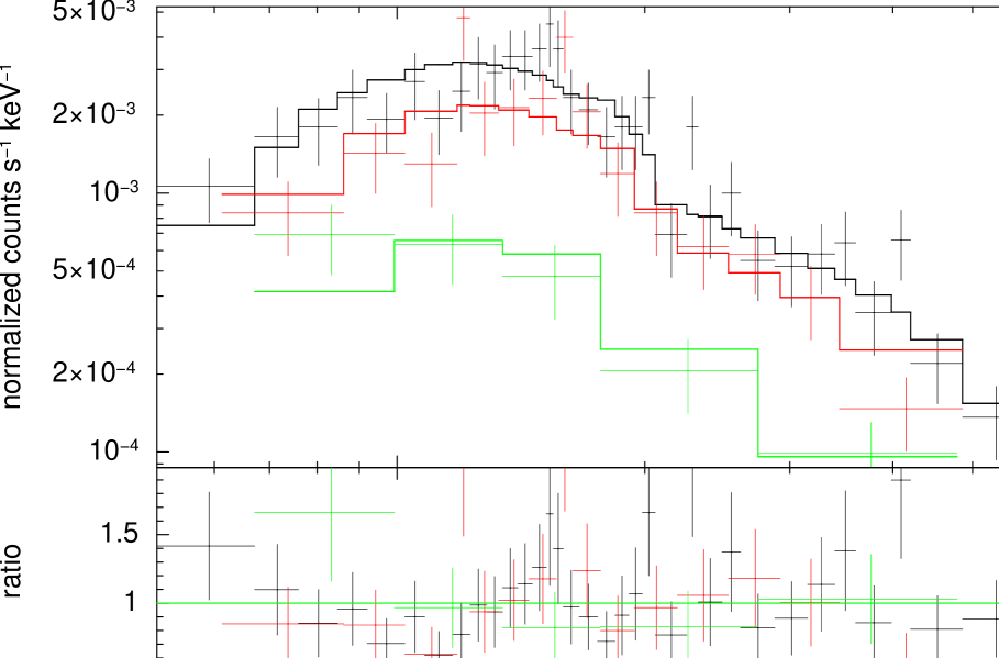
Figure 1: Data and residuals for the best-fit absorbed power law for the three Chandra observations. Top (black) obs. no. 2019, middle (red) no. 9531, bottom (green) no. 9807.

The count rate between the three observations varies. In order to avoid complications in comparing count rates of observations taken in FAINT and VFAINT modes, we evaluate this variability with a simple absorbed power law model (${\tt wabs*powerlaw}$). Despite its simplicity, it is informative of some basic parameters useful to our further analysis. Separate fits of each observation return comparable values of the absorption column $n_{H}$ and the spectral photon index $\Gamma$. For this reason we tie $n_{H}$ and $\Gamma$ of each data set to a common value and fit them simultaneously. Table 2 summarises the results of the fit, and Figure 1 shows the model and its residuals. The value of the C-statistics is $C/{\rm dof}=100.8/101$. The best fitting absorption column is $n_{H}=3.7_{-1.0}^{+1.0}\times 10^{21}{\leavevmode\nobreak\ \rm cm}^{-2}$, and the spectral photon index is $\Gamma=1.88_{-0.24}^{+0.25}$, both consistent with those presented by Wolter & Trinchieri (2004). The value of $n_{H}$ is higher than Galactic, but consistent both with other X-ray measures in the Cartwheel and with the intrinsic absorption in the optical band (see Wolter & Trinchieri, 2004).

The intrinsic luminosities in the spectral band $0.5-10{\leavevmode\nobreak\ \rm keV}$ is $1.2\times 10^{41}{{\leavevmode\nobreak\ \rm erg}\;\rm s^{-1}}$, $8.6\times 10^{40}{{\leavevmode\nobreak\ \rm erg}\;\rm s^{-1}}$ and $2.8\times 10^{40}{{\leavevmode\nobreak\ \rm erg}\;\rm s^{-1}}$ for the first, second and third observation respectively. Compared to the Eddington luminosity of a $1{\leavevmode\nobreak\ M_{\odot}}$ collapsed object, these luminosities seem to imply a black hole of $\gtrsim 200{\leavevmode\nobreak\ M_{\odot}}$. It is perhaps worth to remark that the Eddington luminosity is bolometric, while in the present paper we refer to the luminosity in the X–ray band. This is an approximation of the bolometric luminosity within a factor $\gtrsim 2$.

Formally, a power law model provides an adequate description of the Chandra data sets, and more refined models are not statistically required. Nevertheless, we would like to know whether these observations may somehow constrain some of the theoretical models suggested for the ULXs. The following sections aim at this goal.

4 The Accretion Models

In the framework of an accretion scenario, the engine of N10 is a black hole accreting mass from a donor star through a disc. In this section we present the results of the spectral analysis of three accretion models: i) a multi–colour disc (diskbb in the language of XSPEC), ii) a model of a disc around a maximally rotating Kerr black hole ($\tt kerrd$ in XSPEC) and finally iii) a Kawaguchi (2003) slim disc model . All models are acceptable on statistical grounds and they all return similar values of the C-stat. For an easier comparison, we have summarised the results of these models in Table 3. We also shall discuss the hyperaccretion model suggested by King et al. (2001), but since no spectral model is available for this, our discussion will be mainly qualitative.

4.1 The multicolour disc

The first model we consider is a multicolour disc (MCD) modified by the interstellar absorption. The two free parameters of the model are the effective temperature of the inner rim $T_{\rm in}$ and the apparent inner disc radius $R_{\rm in}$, related to the actual inner radius $R_{\rm disc}$ through the relation (Kubota et al., 1998)

$$R_{\rm disc}=\xi\;f^{2}\;R_{\rm in},$$ (1)

where $\xi\simeq 0.412$ is a correction factor that takes into account that the maximum temperature $T_{\rm in}$ does not occur exactly at the inner edge of the disc (Kubota et al., 1998). For typical parameters, the disc optical opacity is dominated by electron scattering. The electron scattering may also Comptonise the emerging spectrum, and this effect is taken into account by introducing the so called hardening factor $f$, i.e. the ratio $f\equiv T_{\rm col}/T_{\rm eff}$ between the colour temperature $T_{\rm col}$ and the effective temperature $T_{\rm eff}$. The value of $f$ is insensitive to the disc viscosity and the mass of the accretor, but is sensitive to the mass accretion rate. For a mass accretion rate close to the Eddington limit the value of $f$ lies in the range $f\simeq 1.7-2.0$ (Shimura & Takahara, 1995). Kawaguchi (2003) argues that if the accretion rate largely exceeds the Eddington limit (${\dot{M}}\,c^{2}/L_{\rm Edd}>100$), the hardening factor is somewhat larger, in the range $f\simeq 2.3-6.5$. Introducing the radiation efficiency

$$\eta=L/{\dot{M}}c^{2},$$ (2)

this limit translates into

$$L>100\,\eta\>L_{\rm Edd}.$$ (3)

For a disc accreting on a Schwarzschild black hole $\eta\simeq 0.06$ (Frank et al., 2002), so Kawaguchi’s hardening parameter applies if $L\gtrsim 6\,L_{\rm Edd}$.

The normalisation of the model only involves geometrical parameters, so we link the normalisation of the three spectra to a common value, and leave the disc temperatures free to vary. Since the absorption columns inferred from each spectrum are consistent, we also link them to a common value. The interstellar absorption column is $n_{H}=1.8_{-0.6}^{+0.6}\times 10^{21}{\leavevmode\nobreak\ \rm cm}^{-2}$. The disc inner temperature is $T_{\rm in}=1.33_{-0.17}^{+0.22}{\leavevmode\nobreak\ \rm keV}$ for the first observation; $T_{\rm in}=1.21_{-0.16}^{+0.17}{\leavevmode\nobreak\ \rm keV}$ for the second observation and $T_{\rm in}=0.89_{-0.11}^{+0.14}{\leavevmode\nobreak\ \rm keV}$ for the third observation. The normalisation of the model is $K=7.4_{-3.3}^{+5.2}\times 10^{-4}$, and is related to the apparent inner radius $R_{\rm in}$ through the expression

$$R_{\rm in}=1.22\times 10^{2}{\leavevmode\nobreak\ \rm km}\;\left(\frac{K}{10^{-4}}\right)^{1/2}\;\left(\frac{D}{122{\leavevmode\nobreak\ \>\rm Mpc}}\right)\;\bigl{(}\cos\theta\bigr{)}^{-1/2},$$ (4)

where $\theta$ is the inclination of the disc with respect to the line of sight ($\theta=0$ is face–on), and $D$ is the distance to the source. Inserting the appropriate value of $K$ we find

$$R_{\rm disc}\simeq 3.3_{-0.8}^{+1.0}\times 10^{2}\;\xi\;f^{2}/(\cos\theta)^{1/2}\;{\leavevmode\nobreak\ \rm km}.$$ (5)

If the inner edge of the disc is located at the last stable orbit of a Schwarzschild black hole, this implies

$$M_{\bullet}\simeq 61_{-12}^{+18}{\leavevmode\nobreak\ M_{\odot}}\;\left(\frac{f}{2.0}\right)^{2}\;\left(\frac{\xi}{0.41}\right)\;\frac{1}{(\cos\theta)^{1/2}}.$$ (6)

The resulting disc luminosities are $L_{1}=4.1\times 10^{40}{{\leavevmode\nobreak\ \rm erg}\;\rm s^{-1}}$, $L_{2}=2.7\times 10^{40}{{\leavevmode\nobreak\ \rm erg}\;\rm s^{-1}}$ and $L_{3}=8.0\times 10^{39}{{\leavevmode\nobreak\ \rm erg}\;\rm s^{-1}}$, for the first, second and third observation, respectively. All these values exceed the Eddington luminosity $L_{\rm Edd}\simeq 7.9\times 10^{39}{{\leavevmode\nobreak\ \rm erg}\;\rm s^{-1}}$ for a black hole of $M_{\bullet}\simeq 60{\leavevmode\nobreak\ M_{\odot}}$ by a factor $L/L_{\rm Edd}\lesssim 5$, consistent with our choice of the hardening parameter $f=2$.

A long–standing problem of the application of MCD models to the ULXs is that they tend to overestimate the disc’s inner temperature $T_{\rm in}$. Indeed, the luminosity of a MCD is (Kubota et al., 1998)

$$L_{\rm bol}=4\,\pi\>\left(\frac{R_{\rm disc}}{\xi}\right)^{2}\>\sigma_{\rm SB}\;\left(\frac{T_{\rm in}}{f}\right)^{4}$$ (7)

(Makishima et al., 2000). If the temperature is too high (for the same luminosity and the other parameters), the disc radius $R_{\rm disc}$ is underestimated, so is the black hole’s mass. A possible explanation for this effect is the presence of a hot corona embedding the disc (Stobbart et al., 2006): a single MCD model applied to such system would return spuriously high disc temperatures. We investigate how the presence of a hot corona would affect our estimate (6) of the black hole mass. We describe N10 with a Comptonised disc emission, where the temperature of the Compton seed photons is set equal to the disc inner temperature. On account of our rather low statistics, the temperature of the hot corona is not well constrained, and it has been fixed to $k_{B}T_{C}=50{\leavevmode\nobreak\ \rm keV}$, while its optical depth has been left free to vary. The best-fitting value of the Compton thickness is $\tau\simeq 0.5_{-0.2}^{+0.4}$: this results strongly depends on the temperature $T_{C}$, with cooler coronae returning larger optical depths. The temperature of the disc, however, is not sensitive to the precise values of $T_{C}$ and $\tau$. As noted by Stobbart et al. (2006), a Compton–thick ($\tau>1$) corona obscures the inner region of the disc, and in this case the MCD parameters cannot provide reliable estimates of the black hole’s mass (see also Gladstone et al., 2009). The disc temperature of the three observations are respectively $T_{\rm in}=0.53_{-0.12}^{+0.11}{\leavevmode\nobreak\ \rm keV}$, $T_{\rm in}=0.36_{-0.09}^{+0.16}{\leavevmode\nobreak\ \rm keV}$ and $T_{\rm in}=0.09_{-0.04}^{+0.05}{\leavevmode\nobreak\ \rm keV}$. The normalisation of the disc component is $K=7.6_{-3.9}^{+10.6}\;\times 10^{-3}$ (in XSPEC units), yielding

$$M_{\bullet}=141_{-42}^{+78}{\leavevmode\nobreak\ M_{\odot}}\;\left(\frac{\xi}{0.41}\right)\;\left(\frac{f}{1.7}\right)^{2}$$ (8)

Using the above disc inner temperatures we infer the luminosity of the disc component to be $L_{1}=9.0\times 10^{39}{{\leavevmode\nobreak\ \rm erg}\;\rm s^{-1}}$ (first observation), $L_{2}=1.5\times 10^{39}{{\leavevmode\nobreak\ \rm erg}\;\rm s^{-1}}$ (second observation) and $L_{3}=5\times 10^{35}{{\leavevmode\nobreak\ \rm erg}\;\rm s^{-1}}$ (last observation). The ratio between $L_{1}$ and the Eddington luminosity of a black hole of $M_{\bullet}\simeq 141{\leavevmode\nobreak\ M_{\odot}}$ is $\sim 0.5$, which justifies our choice $f=1.7$ of the hardening parameter. As expected (see Stobbart et al., 2006), a hot corona lowers our estimate of disc’s temperature and increases the black hole’s mass with respect to a simple MCD model.

4.2 The Kerr disc

The second model we consider is the spectrum emitted by a disc orbiting a maximally rotating Kerr black hole. We fix the distance of the Cartwheel to its known value, and the hardening parameter to $f=1.7$: the quality of our fit is independent of this choice. The inclination of the disc with respect to the line of sight has been fixed to $\theta=0^{\circ}$; the value of $\theta$ affects the determination of $M_{\bullet}$, as we shall discuss at the end of this section. We also set the radius of the accretion disc to the last stable orbit of a maximally rotating Kerr BH ($\simeq 1.235\,G\,M_{\bullet}/c^{2}$), and the disc outer radius to its default value (the model is insensitive to this parameter). The only free parameters of the model (apart from the hydrogen column density) are the mass $M_{\bullet}$ of the central object and its mass accretion rate $\dot{M}$. In the fitting procedure we link all the parameters for the three observations except the mass accretion rates.

The fit returns the absorption column $n_{H}=2.2_{-0.6}^{+0.6}\times 10^{21}{\leavevmode\nobreak\ \rm cm}^{-2}$, and the mass of the central object results

$$M_{\bullet}=92.8_{-27.7}^{+32.4}{\leavevmode\nobreak\ M_{\odot}}.$$ (9)

The luminosity of the source is $L_{1}=4.3\times 10^{40}$ in the first observation, $L_{2}=2.9\times 10^{40}$ in the second, and $L_{3}=8.5\times 10^{39}$ in the last. The Eddington luminosity associated to the mass (9) is $L_{\rm Edd}=1.2\times 10^{40}{{\leavevmode\nobreak\ \rm erg}\;\rm s^{-1}}$. These values must be checked for their consistency with the adopted hardening parameter. A Kerr maximally rotating black hole has an accretion efficiency $\eta\sim 0.4$ (Frank et al., 2002, see Equation 2). Kawaguchi’s larger values of $f$ then apply if $L\gtrsim 40\,L_{\rm Edd}$. In all our observations, the Kerr disc model returns $L/L_{\rm Edd}\lesssim 3.5$, so the adopted hardening parameter is consistent with the inferred $M_{\bullet}$ and the relatively low mass accretion regime.

Before ending this section we need to address the effect of the disc inclination $\theta$ on the estimate of the mass $M_{\bullet}$. The value of $\theta$ does not affect the quality of the fit, but the mass is sensitive to it, as shown in Figure 2 (see also Hui & Krolik, 2008). Low inclination angles imply lower $M_{\bullet}$, which (for $f=1.7$) attains a minimum value of $\sim 77{\leavevmode\nobreak\ M_{\odot}}$ for $\theta=20^{\circ}$. If the disc is seen almost edge–on, on the other hand, $M_{\bullet}$ grows up to $M_{\bullet}\simeq 10^{3}{\leavevmode\nobreak\ M_{\odot}}$. This trend of $M_{\bullet}$ with the viewing angle is also found in the multicolour discs considered in the previous section (in particular, see Equation 6).

To summarise, the Kerr disc model is consistent with a black hole of $M_{\bullet}\simeq 90{\leavevmode\nobreak\ M_{\odot}}$, similar (within the uncertainties) to what inferred from the Comptonised multicolour disc model. Higher masses are not excluded, if the disc is highly tilted with respect to the line of sight. Also a higher hardening factor would increase $M_{\bullet}$, but higher values of $f$ are not required by the inferred accretion regime.

4.3 Slim Discs

The multicolour disc model assumes that the disc radiates locally as a black body. If the accretion rate largely exceeds the Eddington limit, this hypothesis is not appropriate. In such an accretion regime the heat content of the disc is trapped and dragged to the black hole’s horizon before it is radiated. For this reason, slim discs are radiatively inefficient, and their properties significantly differ from those of the standard thin discs (see e.g. Abramowicz et al., 1988; Frank et al., 2002). In this section we investigate whether the data support the possibility that N10 is powered by a slim disc accreting above its Eddington limit.

In XSPEC two slim disc models are available: we adopted the model based on the calculation by Kawaguchi (2003), with the mass of the central object, the accretion rate and the viscosity $\alpha$ as free parameters. The spectrum is calculated taking into account the local Comptonisation and the relativistic effects. Kawaguchi’s model has been applied to fit the XMM–Newton spectra of some ULXs (see e.g. Okajima et al., 2006; Vierdayanti et al., 2006), returning black hole masses of few tens of ${\leavevmode\nobreak\ M_{\odot}}$ accreting at super–Eddington regimes. In our fit we have linked the interstellar absorption column, the hole mass and the $\alpha$ parameter between the observations. The mass accretion rate is independent for each observation. The fitting procedure is unable to constrain the black hole’s mass. The confidence regions are open for $M_{\bullet}\gtrsim 80{\leavevmode\nobreak\ M_{\odot}}$ (Figure 3), and the model is consistent with any value of $M_{\bullet}$ above this limit. The absorption column is $n_{H}=3.6_{-0.9}^{+0.7}\times 10^{21}{\leavevmode\nobreak\ \rm cm}^{-2}$, while the viscosity parameter and the BH mass are $\alpha=0.56_{-0.37}$ and $M_{\bullet}=495_{-340}{\leavevmode\nobreak\ M_{\odot}}$ respectively. The mass accretion rates for the three observations are ${\dot{M}}_{1}=39.4_{-23}$, ${\dot{M}}_{2}=21.4_{-12.0}^{+523}$, ${\dot{M}}_{3}=5.1_{-1.2}^{+79}$, all in units of ${\dot{M}}_{\rm Edd}\equiv L_{\rm Edd}/c^{2}$. Assuming the conversion factor ${\dot{M}}_{\rm Edd}=1.3\times 10^{19}\leavevmode\nobreak\ {\rm g}{\leavevmode\nobreak\ \rm s}^{-1}(M_{\bullet}/100{\leavevmode\nobreak\ M_{\odot}})$ used by Kawaguchi (2003), the best fitting accretion rates are $\dot{M}_{1}=2.5\times 10^{21}\leavevmode\nobreak\ {\rm g}{\leavevmode\nobreak\ \rm s}^{-1}$, $\dot{M}_{2}=1.4\times 10^{21}\leavevmode\nobreak\ {\rm g}{\leavevmode\nobreak\ \rm s}^{-1}$, $\dot{M}_{3}=3.3\times 10^{20}\leavevmode\nobreak\ {\rm g}{\leavevmode\nobreak\ \rm s}^{-1}$. It is not possible to set upper limits to the the parameters $\alpha$, $M_{\bullet}$ and $\dot{M}_{1}$, since the error calculation hits the limits of their tabulated values ($\alpha=1$, $M_{\bullet}=1000{\leavevmode\nobreak\ M_{\odot}}$ and $\dot{M}=1000\leavevmode\nobreak\ {\dot{M}}_{\rm Edd}$, respectively).

One caveat is in order about the consistency of the application of slim disc models to N10. The radial temperature profile of slim discs varies as $T\propto R^{-1/2}$ instead of $T\propto R^{-3/4}$ characteristic of thin multicolour discs (Watarai et al., 2000). The radial dependence of $T_{\rm in}$ in N10 may be checked with a multicolour disc (diskpbb in XSPEC) where the temperature index $p$ (defined by $T(R)\propto R^{-p}$) is a free parameter. The index $p\simeq 0.5$ has been found in some ULX spectra successfully fitted with a slim disc model (Okajima et al., 2006; Vierdayanti et al., 2006). In our case the model wabs*diskpbb is comparable to the others and since its best–fitting parameters are very similar to those derived from a standard multicolour disc, we do not present them. Our best fitting value is $p\simeq 0.74_{-0.19}^{+3.66}$ close to the standard value $0.75$, but slightly inconsistent with the slim disc value $p=0.5$.

4.4 The “Hyperaccretion” model

The last accretion model we consider for N10 is the so–called “hyperaccretion” scenario (King et al., 2001; King, 2008, 2009). This model explains the high luminosity of the ULXs with a combination of a high accretion rate (close to the Eddington limit) on a stellar mass black hole, and a mechanical beaming due to the accretion stream itself.

The apparent X–ray luminosity (Equation (10) in King, 2009) of the source results

$$L\simeq 2.2\times 10^{36}{{\leavevmode\nobreak\ \rm erg}\;\rm s^{-1}}\;\left(\frac{M_{\bullet}}{{\leavevmode\nobreak\ M_{\odot}}}\right)\;\left(\frac{\dot{M}}{\dot{M}_{\rm Edd}}\right)^{2}\;\left[1+\ln\left(\frac{\dot{M}}{\dot{M}_{\rm Edd}}\right)\right]$$ (10)

where $\dot{M}$ is the mass transfer rate from the donor star and $\dot{M}_{\rm Edd}=L_{\rm Edd}/\eta\,c^{2}$ is the Eddington–limited mass transfer, dependent on the efficiency $\eta$ of the X–ray production in the accretion process, defined by Equation (2).

One of the most relevant features of this model is that the beaming factor scales as ${\dot{M}}^{-2}$. This causes the bolometric luminosity to scale with the disc’s temperature as

$$L\propto T_{\rm in}^{-4},$$ (11)

opposite to the standard correlation $L\propto T_{\rm in}^{4}$.

The prediction (11) has been found consistent with the $L-T_{\rm in}$ relation of the soft excess observed in some ULXs (Feng & Kaaret, 2007; Kajava & Poutanen, 2009; Gladstone et al., 2009). We assume that the count rate of N10 correlates with its intrinsic luminosity in all our observations. In principle, it is certainly true that a strong spectral change may alter (even reverse) this correlation, but such a variation of the spectrum of N10 is not supported by our data. Under this working hypothesis, we measure a positive correlation between the inner temperature and the luminosity, at odds with the prediction of the hyperaccretion model. The hyperaccretion scenario probably is not the correct explanation for the nature of N10.

5 The Supernova Model

As discussed in the introduction, accretion power is not the only viable explanation for the ULXs’ engine. Alternative models are possible, and young SNe interacting with their surroundings may explain an appreciable fraction of the known ULXs (Swartz et al., 2004). In this section we investigate the SN model for N10, aiming at deriving the spectral parameters.

The X–ray emission from supernovae may start up to about one year after the explosion, and it is powered by the interaction of the ejecta with the circumstellar medium (CSM, see e.g. Immler & Lewin, 2003). Shock fronts form as the ejecta expand through the CSM. The leading (or “forward”) shock heats the CSM up to $10^{9}-10^{10}\leavevmode\nobreak\ \rm K$, and gradually an inner (or “reverse”) shock wave starts to propagate. The density behind the reverse shock is $5-10$ times higher than that behind the forward shock, and the temperature is lower, around $10^{7}-10^{8}\leavevmode\nobreak\ \rm K$ (Chevalier & Fransson, 1994). For this reason, the soft X–ray emission (below $\lesssim 5{\leavevmode\nobreak\ \rm keV}$) is dominated by the reverse shock, and is well modelled by thermal models, while the hard emission (say, above $10{\leavevmode\nobreak\ \rm keV}$) is dominated by the forward shock.

The luminosities of X–ray supernovae lie in the range $10^{37}-10^{41}{{\leavevmode\nobreak\ \rm erg}\;\rm s^{-1}}$, with the so–called SN IIn supernovae at the bright end of the interval. These are core–collapse supernovae, owing the “n” in their name to the presence of several narrow emission lines in their optical spectrum (Turatto, 2003). These lines are most likely due to the interaction of the ejecta with a dense, slow wind emitted by the SN progenitor. Other supernovae explode in thinner environments, resulting in dimmer X–ray luminosties. For this reason, if N10 is actually a young SN, it is most likely a SN IIn.

We fit the spectra of N10 with the thermal models apec and nei, corrected for interstellar absorption. The apec model assumes that the emitting plasma is in full collisional equilibrium: there is a dynamic balance between the collisional ionisation and the electronic recombination. The nei model does not assume collisional equilibrium, allowing a mismatch between the collisional ionisation and the (longer) recombination process. This mismatch may prevail in shocked plasmas, where the electrons were energised but did not yet settle to collisional equilibrium with the ions (see e.g. Dopita & Sutherland, 2003). The parameters of the nei model are very similar to those derived for the apec model (the fit is quite insensitive to the ionisation age), so we present only the apec results.

In our model (wabs*apec) the absorption column and the metal abundances of the three observations are linked together. Since there is no compelling statistical evidence of a variation of the temperature, we also link together the temperatures of the three observations. The results of this model are presented in Table 4. The statistics of the fit is $C/{\rm dof}=95.9/100$, and the values of the best–fitting parameters are $n_{H}=2.8_{-0.6}^{+0.8}\times 10^{21}{\leavevmode\nobreak\ \rm cm}^{2}$, $k_{B}T=5.1_{-1.6}^{+3.1}{\leavevmode\nobreak\ \rm keV}$, $N_{1}=4.3_{-1.2}^{+0.9}\times 10^{-5}$ (normalisation of the first observation), $N_{2}=3.1_{-0.9}^{+0.7}\times 10^{-5}$ (normalisation of the second observation), and $N_{3}=1.0_{-0.2}^{+0.3}\times 10^{-5}$ (normalisation of the third observation). The units of these quantities are (for sources at low redshift) $10^{-14}\;\int dVn_{e}\;n_{H}/4\,\pi\,D^{2}$, where $D$ is the distance to the source, $n_{e}$ and $n_{H}$ are the electron and proton densities of the emitting plasma, and the integral (known as emission integral) is extended over the volume occupied by the source. The emission integrals are consistent with the size (few $10^{15}{\leavevmode\nobreak\ \rm cm}$) and the density ($\sim 10^{-15}-10^{-16}\leavevmode\nobreak\ \rm g{\leavevmode\nobreak\ \rm cm}^{-3}$) expected from the reverse shock of a young supernova remnant few years after the explosion (see e.g. Chevalier & Fransson, 2003).

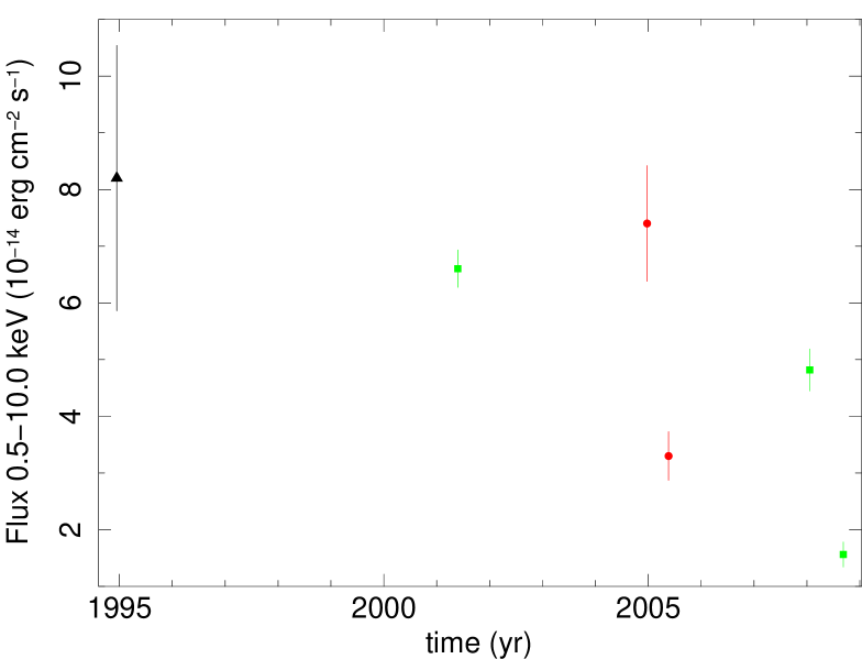
Figure 4: The light curve of the source N10. Fluxes have been calculated with a power-law model corrected for the interstellar absorption. The symbols refer to ROSAT data (triangle) XMM–Newton (circles) and Chandra (squares). ROSAT and XMM–Newton data are taken from Wolter et al. (2006).

The unabsorbed light curve of N10, calculated according to the power law model, is plotted in Figure 4 (see also Wolter et al., 2006). The evolution of the observed flux cannot be fitted by a power law, as observed in other X–ray supernovae (1986J, Houck et al., 1998; 1988Z, Schlegel & Petre, 2006; 1998S, Pooley et al., 2002). This is not an argument against the SN nature of N10, though, since a simple power–law decline of the X–ray luminosity has not been reported in other confirmed SN IIn. SN 1995N, for instance, shows a complex light curve, possibly resulting from the interaction of the ejecta with a complex circumstellar medium (Zampieri et al., 2005). The sudden decrease of the X–ray luminosity of N10 in 2008 might show that the ejecta have passed the dense region of the pre–supernova wind, and have finally reached a low density outer environment.

SN IIn are usually found in high metal environments (1986J, Houck et al., 1998; 1998S, Pooley et al., 2002). Indeed, high metal abundances favour the blowing of the line–driven strong pre–supernova winds required to set up the dense circumstellar environment required to power a stronger X–ray emission. The metallicity of the Cartwheel is low as measured from the HII regions (Fosbury & Hawarden, 1977); the X-ray measure is poorly constrained, and consistent with zero. Therefore the SN progenitor had to be quite massive to blow dense enough winds without the aid of a high metallicity.

6 Discussion and Summary

In this paper we considered the spectral modelling of the ULX N10, located in the Cartwheel galaxy in order to assess the nature of this source. Although the source is intrinsically very bright, the spectra have few counts on account of the large distance ($122{\leavevmode\nobreak\ \>\rm Mpc}$). For this reason, we are unable to reject (or confirm) a model on purely statistical grounds. We first discussed several accretion models (multicolour disc around a Schwarzschild or Kerr black hole, slim disc, hyperaccretion). All models indicate a black hole of $\sim 100{\leavevmode\nobreak\ M_{\odot}}$, at the high end of the mass distribution of a black hole generated by stellar evolution, possibly in a metal poor environment. This result is consistent with the conclusions of Mapelli et al. (2009) and Zampieri & Roberts (2009) that stellar evolution in a metal depleted environment may produce black holes of $30-90{\leavevmode\nobreak\ M_{\odot}}$.

The theoretical studies of the evolution of very massive stars have been rekindled by the discovery of the ULXs, with the result that black holes of $\sim 100{\leavevmode\nobreak\ M_{\odot}}$ are more common than earlier works suggested. Isolated solar–abundance stars may have masses up to $150{\leavevmode\nobreak\ M_{\odot}}$, but in dense environments they may coalesce to form stars as massive as $1000{\leavevmode\nobreak\ M_{\odot}}$ (Yungelson et al., 2008). Recent studies on the mass loss from hot, massive stars (Puls et al., 2008, and references therein) have shown that the occurrence of weak and/or clumpy winds may reduce the mass loss up by a factor $10$, thus allowing the star to retain a higher fraction of its original mass at the end of its life. Also lower metallicities entail weaker wind mass losses (Heger et al., 2003). Zero metallicity (Population III) stars may be significantly more massive than solar–abundance stars (Ohkubo et al., 2006). All these factors determine the mass of the final black hole, that may range from $\sim 70{\leavevmode\nobreak\ M_{\odot}}$ for a solar–abundance progenitor (Yungelson et al., 2008), up to $500{\leavevmode\nobreak\ M_{\odot}}$ for low metallicity stars (Ohkubo et al., 2006). Observations indicate that the low metallicity scenario is more likely for N10: the Cartwheel galaxy is metal–poor, and although the available measurements (Fosbury & Hawarden, 1977) are not at the exact location of N10, they should nevertheless be representative of the average abundance in the ring. We therefore conclude that the interpretation of N10 as a black hole of $\sim 100{\leavevmode\nobreak\ M_{\odot}}$ suggested by the X–ray data is consistent with the theoretical predictions of the evolution of massive stars in a dense environment.

In summary, if ordinary stellar evolution is the correct scenario to form the black hole, N10 could be an extreme High Mass X–ray Binary (HMXB). The mass accretion rate $\dot{M}$ on the black hole may be inferred from the luminosity $L$ via Equation (2), and is of the order of ${\dot{M}}\simeq 10^{-6}\leavevmode\nobreak\ {\leavevmode\nobreak\ M_{\odot}}{\leavevmode\nobreak\ \rm yr}^{-1}$. This value is comparable with the loss rate of massive (i.e., few tens solar masses, Frank et al., 2002) donor stars on a thermal time scale. The accretion flow from the donor star to the BH is most likely to occur through a Roche lobe overflow; the BH capture of a wind blown by the companion is less favoured, since the small capture radius would require an unlikely strong mass loss from the companion.

Can the observed decay of the luminosity of the source be explained in the framework of the accretion model? The longest characteristic time of an accretion disc is the so–called “viscous time” $t_{\rm visc}$, i.e. the characteristic time taken by the disc to adapt to new conditions. For a standard $\alpha$-disc orbiting a black hole of $100{\leavevmode\nobreak\ M_{\odot}}$ with an accretion rate ${\dot{M}}\simeq 10^{-6}\leavevmode\nobreak\ {\leavevmode\nobreak\ M_{\odot}}{\leavevmode\nobreak\ \rm yr}^{-1}$, $t_{\rm visc}\simeq 10^{2}-10^{3}{\leavevmode\nobreak\ \rm s}$ (Frank et al., 2002), much shorter than the time scale of the variability of N10 (few years). Therefore, the observed variability cannot be due to a sort of disc instability, which would affect the disc and the luminosity of the source over a time scale $t_{\rm visc}$. The simplest alternative is that the variability is due to a change of the mass transfer rate from the donor star. This may be due to an intrinsic decay of the mass loss from the donor, but also to other effects occurring at the inner Lagrangian point, since the instantaneous mass flow here is very sensitive to the relative sizes of the donor star and the Roche lobe (Frank et al., 2002). New observations of this interesting source would help to settle the question.

We also explored the possibility that N10 is a young supernova strongly interacting with the circumstellar medium. Both the interpretation of this model and the best–fitting spectral parameters are consistent with this view. A new flux brightening of the source in the future would rule out this hypothesis.

Figure 2: The best–fitting mass $M_{\bullet}$ of the model ${\tt wabs*kerrd}$ as a function of the inclination $\theta$ between the disc and the line of sight. The error bars represent the $90\%$ uncertainties calculated with the free parameters.

Figure 3: The dependence of the fit C-statistics on the black hole mass in the slim disc model by Kawaguchi (2003). Since the C-statistics curve is flat for $M_{\bullet}\gtrsim 80{\leavevmode\nobreak\ M_{\odot}}$, the best–fitting mass of the hole can be anywhere above this value.

Table 1: Chandra observation log of the Cartwheel galaxy.

Observation	Exposure time	Count rate	Mode	Start date
identification	(before) after cleaning	($0.3-7{\leavevmode\nobreak\ \rm keV}$)
	(ks)	($10^{-3}$ cts/s)		(yyyy/mm/dd)
2019	(76.5) 76.1	$5.3$	FAINT	2001/05/26
9531	(52.8) 48.0	$3.6$	VFAINT	2008/01/21
9807	(49.8) 49.5	$1.2$	VFAINT	2008/09/09

Table 2: Summary of the absorbed power–law model ($\tt wabs*powerlaw$).

Obs. id.	Normalisation	$F_{0.5-10{\leavevmode\nobreak\ \rm keV}}$	$L_{0.5-10{\leavevmode\nobreak\ \rm keV}}$
	$10^{-5}$ XSPEC units	($10^{-14}{{\leavevmode\nobreak\ \rm erg}\;\rm s^{-1}}{\leavevmode\nobreak\ \rm cm}^{-2}$)	($10^{40}{{\leavevmode\nobreak\ \rm erg}\;\rm s^{-1}}$)
2019	$1.24_{-0.27}^{+0.36}$	$6.60$	$11.8$
9531	$0.91_{-0.21}^{+0.27}$	$4.81$	$8.6$
9807	$0.29_{-0.08}^{+0.11}$	$1.56$	$2.8$
$n_{H}=3.67_{-0.93}^{+0.99}\times 10^{21}{\leavevmode\nobreak\ \rm cm}^{-2}$	$\Gamma=1.88_{-0.24}^{+0.25}$	$C/{\rm dof}=100.8/101$

Table 3: Summary of the accretion disc models: MCD=wabs*diskbb, MCD+C=wabs*(diskbb+comptt), Kerr=wabs*kerrd Slim=wabs*Kawaguchi. The first group of rows shows the best–fitting parameters for three observations separately. The second groups presents the values of the parameters common to all the observations, and the other parameters discussed in the text. Fluxes and luminosities are calculated in the spectral band $0.5-10{\leavevmode\nobreak\ \rm keV}$. $K_{D}$ and $K_{C}$ stand for the disc and comptt normalisation, respectively. $f$, $\eta$ and $\theta$ are the hardening parameter, the accretion efficiency and the inclination of the disc. The luminosites are total, so the luminosity of the MCD+C model also includes the contribution of the Compton corona.

Obs. id.	MCD			MCD+C			Kerr			Slim
	$k_{B}T_{\rm in}$	Flux	LX	$k_{B}T_{\rm in}$	Flux	LX	$\dot{M}$	Flux	LX	$\dot{M}$	Flux	LX
	(${\leavevmode\nobreak\ \rm keV}$)	$10^{-14}$	$10^{40}$	(${\leavevmode\nobreak\ \rm keV}$)	$10^{-14}$	$10^{40}$	$10^{20}\leavevmode\nobreak\ \rm g{\leavevmode\nobreak\ \rm s}^{-1}$	$10^{-14}$	$10^{40}$	$L_{\rm Edd}/c^{2}$	$10^{-14}$	$10^{40}$
		${{\leavevmode\nobreak\ \rm erg}\;\rm s^{-1}}{\leavevmode\nobreak\ \rm cm}^{-2}$	${{\leavevmode\nobreak\ \rm erg}\;\rm s^{-1}}$		${{\leavevmode\nobreak\ \rm erg}\;\rm s^{-1}}{\leavevmode\nobreak\ \rm cm}^{-2}$	${{\leavevmode\nobreak\ \rm erg}\;\rm s^{-1}}$		${{\leavevmode\nobreak\ \rm erg}\;\rm s^{-1}}{\leavevmode\nobreak\ \rm cm}^{-2}$	${{\leavevmode\nobreak\ \rm erg}\;\rm s^{-1}}$		${{\leavevmode\nobreak\ \rm erg}\;\rm s^{-1}}{\leavevmode\nobreak\ \rm cm}^{-2}$	${{\leavevmode\nobreak\ \rm erg}\;\rm s^{-1}}$
2019	$1.33_{-0.17}^{+0.22}$	$4.63$	$4.1$	$0.53_{-0.12}^{+0.11}$	$5.32$	$8.6$	$7.1_{-0.7}^{+0.8}$	$4.84$	$4.3$	$39.4_{-23}$	$11.5$	$5.8$
9531	$1.21_{-0.16}^{+0.17}$	$3.09$	$2.7$	$0.36_{-0.09}^{+0.16}$	$3.63$	$6.3$	$4.8_{-0.7}^{+0.8}$	$3.28$	$2.9$	$21.4_{-12}^{+523}$	$8.0$	$4.0$
9807	$0.89_{-0.11}^{+0.14}$	$0.88$	$0.8$	$0.09_{-0.04}^{+0.05}$	$1.13$	$2.0$	$1.5_{-0.3}^{+0.4}$	$0.94$	$0.85$	$5.1_{-1.2}^{+79}$	$2.3$	$1.1$
$n_{H}(10^{21}{\leavevmode\nobreak\ \rm cm}^{-2})$	$1.80_{-0.6}^{+0.6}$			$1.7_{-0.7}^{+0.8}$			$2.26_{-0.60}^{+0.64}$			$3.6_{-0.9}^{+0.7}$
$K_{D}$	$7.4_{-3.3}^{+5.2}\times 10^{-4}$			$7.6_{-3.9}^{+10.6}\times 10^{-3}$			$1$ (fixed)			$6.72\times 10^{-9}$ (fixed)
$K_{C}$	-			$2.27_{-0.6}^{+0.6}\times 10^{-7}$			-			-
$T_{C}$	-			$50{\leavevmode\nobreak\ \rm keV}$ (fixed)			-			-
$\tau$	-			$0.5_{-0.2}^{+0.4}$			-			-
$\theta$	$0$			$0$			$0$			$0$
$\alpha$	-			-			-			$0.56_{-0.37}$
$M_{\bullet}$	-			-			$92.8_{-27.7}^{+32.5}$			$495_{-340}$
$f$	$2.0$			$1.7$			$1.7$			$1.7$
$\eta$	$0.06$			$0.06$			$0.4$			$0.06$
$C/{\rm dof}$	$92.8/101$			$88.5/99$			$93.2/101$			$96.7/100$

Table 4: Summary of the absorbed APEC model wabs* apec.

Obs. identification no.	Normalisation	$F_{0.5-10{\leavevmode\nobreak\ \rm keV}}$	$L_{0.5-10{\leavevmode\nobreak\ \rm keV}}$
	$10^{-5}$ XSPEC units	($10^{-14}{{\leavevmode\nobreak\ \rm erg}\;\rm s^{-1}}{\leavevmode\nobreak\ \rm cm}^{-2}$)	($10^{40}{{\leavevmode\nobreak\ \rm erg}\;\rm s^{-1}}$)
2019	$4.3_{-1.2}^{+0.9}$	$5.55$	$9.9$
9531	$3.1_{-0.9}^{+0.7}$	$4.04$	$7.2$
9807	$1.0_{-0.2}^{+0.3}$	$1.31$	$2.3$
$n_{H}=2.8_{-0.6}^{+0.8}\times 10^{21}{\leavevmode\nobreak\ \rm cm}^{-2}$	$k_{B}\,T=5.1_{-1.6}^{+3.1}{\leavevmode\nobreak\ \rm keV}$	$Z=0^{+0.2}$	$C/{\rm dof}=95.9/100$

References

- Abramowicz et al. (1988) Abramowicz M. A., Czerny B., Lasota J. P., Szuszkiewicz E., 1988, ApJ, 332, 646
- Arnaud (1996) Arnaud K. A., 1996, in G. H. Jacoby & J. Barnes ed., Astronomical Data Analysis Software and Systems V Vol. 101 of Astronomical Society of the Pacific Conference Series, XSPEC: The First Ten Years. pp 17–20
- Begelman (2002) Begelman M. C., 2002, ApJ, 568, L97
- Begelman (2006) Begelman M. C., 2006, ApJ, 643, 1065
- Cash (1979) Cash W., 1979, ApJ, 228, 939
- Chevalier & Fransson (1994) Chevalier R. A., Fransson C., 1994, ApJ, 420, 268
- Chevalier & Fransson (2003) Chevalier R. A., Fransson C., 2003, in Weiler K., ed., Supernovae and Gamma-Ray Bursters Vol. 598 of Lecture Notes in Physics, Berlin Springer Verlag, Supernova Interaction with a Circumstellar Medium. pp 171–194
- Colbert & Mushotzky (1999) Colbert E. J. M., Mushotzky R. F., 1999, ApJ, 519, 89
- Crivellari et al. (2009) Crivellari E., Wolter A., Trinchieri G., 2009, A&A, 501, 445
- Dopita & Sutherland (2003) Dopita M. A., Sutherland R. S., 2003, Astrophysics of the Diffuse Universe. Springer Verlag, Berlin, New York
- Ebisawa et al. (2003) Ebisawa K., Życki P., Kubota A., Mizuno T., Watarai K.-y., 2003, ApJ, 597, 780
- Fabbiano (1989) Fabbiano G., 1989, ARA&A, 27, 87
- Fabbiano (2006) Fabbiano G., 2006, ARA&A, 44, 323
- Feng & Kaaret (2007) Feng H., Kaaret P., 2007, ApJ, 660, L113
- Fosbury & Hawarden (1977) Fosbury R. A. E., Hawarden T. G., 1977, MNRAS, 178, 473
- Frank et al. (2002) Frank J., King A., Raine D. J., 2002, Accretion Power in Astrophysics, third edn. Cambridge University Press, Cambridge, UK
- Gladstone et al. (2009) Gladstone J. C., Roberts T. P., Done C., 2009, MNRAS, 397, 1836
- Heger et al. (2003) Heger A., Fryer C. L., Woosley S. E., Langer N., Hartmann D. H., 2003, ApJ, 591, 288
- Higdon (1996) Higdon J. L., 1996, ApJ, 467, 241
- Houck et al. (1998) Houck J. C., Bregman J. N., Chevalier R. A., Tomisaka K., 1998, ApJ, 493, 431
- Hui & Krolik (2008) Hui Y., Krolik J. H., 2008, ApJ, 679, 1405
- Immler & Lewin (2003) Immler S., Lewin W. H. G., 2003, in Weiler K., ed., Supernovae and Gamma-Ray Bursters Vol. 598 of Lecture Notes in Physics, Berlin Springer Verlag, X-Ray Supernovae. pp 91–111
- Kajava & Poutanen (2009) Kajava J. J. E., Poutanen J., 2009, MNRAS, 398, 1450
- Kawaguchi (2003) Kawaguchi T., 2003, ApJ, 593, 69
- King (2008) King A., 2008, New Astronomy Review, 51, 775
- King (2009) King A. R., 2009, MNRAS, 393, L41
- King et al. (2001) King A. R., Davies M. B., Ward M. J., Fabbiano G., Elvis M., 2001, ApJ, 552, L109
- Kubota et al. (1998) Kubota A., Tanaka Y., Makishima K., Ueda Y., Dotani T., Inoue H., Yamaoka K., 1998, PASJ, 50, 667
- Long & van Speybroeck (1983) Long K. S., van Speybroeck L. P., 1983, in W. H. G. Lewin & E. P. J. van den Heuvel ed., Accretion-Driven Stellar X-ray Sources X-ray emission from normal galaxies. pp 117–146
- Makishima et al. (2000) Makishima K., Kubota A., Mizuno T., Ohnishi T., Tashiro M., Aruga Y., Asai K., Dotani T., Mitsuda K., Ueda Y., Uno S., Yamaoka K., Ebisawa K., Kohmura Y., Okada K., 2000, ApJ, 535, 632
- Mapelli et al. (2009) Mapelli M., Colpi M., Zampieri L., 2009, MNRAS, 395, L71
- Mapelli et al. (2008) Mapelli M., Moore B., Ripamonti E., Mayer L., Colpi M., Giordano L., 2008, MNRAS, 383, 1223
- Miller & Hamilton (2002) Miller M. C., Hamilton D. P., 2002, MNRAS, 330, 232
- Ohkubo et al. (2006) Ohkubo T., Umeda H., Maeda K., Nomoto K., Suzuki T., Tsuruta S., Rees M. J., 2006, ApJ, 645, 1352
- Okajima et al. (2006) Okajima T., Ebisawa K., Kawaguchi T., 2006, ApJ, 652, L105
- Pooley et al. (2002) Pooley D., Lewin W. H. G., Fox D. W., Miller J. M., Lacey C. K., Van Dyk S. D., Weiler K. W., Sramek R. A., Filippenko A. V., Leonard D. C., Immler S., Chevalier R. A., Fabian A. C., Fransson C., Nomoto K., 2002, ApJ, 572, 932
- Portegies Zwart et al. (2004) Portegies Zwart S. F., Baumgardt H., Hut P., Makino J., McMillan S. L. W., 2004, Nature, 428, 724
- Poutanen et al. (2007) Poutanen J., Lipunova G., Fabrika S., Butkevich A. G., Abolmasov P., 2007, MNRAS, 377, 1187
- Puls et al. (2008) Puls J., Vink J. S., Najarro F., 2008, A&AR, 16, 209
- Schlegel & Petre (2006) Schlegel E. M., Petre R., 2006, ApJ, 646, 378
- Shimura & Takahara (1995) Shimura T., Takahara F., 1995, ApJ, 445, 780
- Socrates & Davis (2006) Socrates A., Davis S. W., 2006, ApJ, 651, 1049
- Stobbart et al. (2006) Stobbart A., Roberts T. P., Wilms J., 2006, MNRAS, 368, 397
- Swartz et al. (2004) Swartz D. A., Ghosh K. K., Tennant A. F., Wu K., 2004, ApJS, 154, 519
- Turatto (2003) Turatto M., 2003, in Weiler K., ed., Supernovae and Gamma-Ray Bursters Vol. 598 of Lecture Notes in Physics, Berlin Springer Verlag, Classification of Supernovae. pp 21–36
- Vierdayanti et al. (2006) Vierdayanti K., Mineshige S., Ebisawa K., Kawaguchi T., 2006, PASJ, 58, 915
- Watarai et al. (2000) Watarai K.-y., Fukue J., Takeuchi M., Mineshige S., 2000, PASJ, 52, 133
- Wolter & Trinchieri (2004) Wolter A., Trinchieri G., 2004, A&A, 426, 787
- Wolter et al. (2006) Wolter A., Trinchieri G., Colpi M., 2006, MNRAS, 373, 1627
- Yungelson et al. (2008) Yungelson L. R., van den Heuvel E. P. J., Vink J. S., Portegies Zwart S. F., de Koter A., 2008, A&A, 477, 223
- Zampieri et al. (2005) Zampieri L., Mucciarelli P., Pastorello A., Turatto M., Cappellaro E., Benetti S., 2005, MNRAS, 364, 1419
- Zampieri & Roberts (2009) Zampieri L., Roberts T. P., 2009, MNRAS, 400, 677