Resolvent estimates for normally hyperbolic trapped sets

1. Introduction and statement of results

We give pole free strips and estimates for resolvents of semiclassical operators which, on the level of the classical flow, have normally hyperbolic smooth trapped sets of codimension two in phase space. Such trapped sets are structurally stable – see §1.2 – and our motivation comes partly from considering the wave equation for slowly rotating Kerr black holes, whose trapped photon spheres have precisely that dynamical structure – see §2. From the semiclassical point of view an example to keep in mind is given by

$$P(z)=-h^{2}\Delta+V(x)-1-z\,,\ \ V\in{\mathcal{C}}^{\infty}_{c}({\mathbb{R}}^{n};{\mathbb{R}})\,,$$

with the classical flow described by Newton’s equations:

$$x^{\prime}(t)=2\xi(t)\,,\ \ \xi^{\prime}(t)=-V^{\prime}(x(t))\,,\ \ \varphi^{t}(x(0),\xi(0))\stackrel{{\scriptstyle\rm{def}}}{{=}}(x(t),\xi(t))\,.$$

The incoming and outgoing tails, $\Gamma_{\pm}$, and the trapped set, $K$, are defined by

$$\Gamma_{\pm}=\{(x,\xi)\;:\;\exists\,M,\ |\varphi^{t}(x,\xi)|\leq M\,,t\rightarrow\mp\infty\}\,,\ \ K\stackrel{{\scriptstyle\rm{def}}}{{=}}\Gamma_{+}\cap\Gamma_{-}\,.$$

As explained in §2 it is important to consider more general families of operator pencils. The general assumptions will be given in §1.1 but the result is already non-trivial in the case presented above: $X={\mathbb{R}}^{n}$, and $P(z)=P-z$, $P=-h^{2}\Delta+V(x)-1$.

Theorem 1.

Suppose that $P(z)$ is a family of operators satisfying the assumptions in §1.1, with a trapped set $K$ which is smooth and normally hyperbolic in the sense of §1.2 and contained in $U_{1}\Subset X.$

If the symbol of $\partial_{z}P(0)$ is strictly negative near $p^{-1}(0)\cap T_{U_{2}}^{*}X$ and $W\in{\mathcal{C}}^{\infty}(X;{\mathbb{R}})$ satisfies

$$W\geq 0\,,\ \ \ W\!\!\restriction_{U_{1}}=0\,,\ \ \ W\!\!\restriction_{X\setminus U_{2}}=1\,,$$

where $\pi(K)\subset\overline{U_{1}}\subset U_{2}\Subset X$ then there exist $\delta_{0},\nu_{0}>0$ such that for $|z|<\delta_{0}$ we have

(1.1) $$\|(P(z)-iW)^{-1}\|_{L^{2}\rightarrow L^{2}}\ \lesssim\ \begin{cases}1/\mathop{\rm Im}\nolimits z\,,&\mathop{\rm Im}\nolimits z>0\,,\\ h^{-1}\log(1/h)\,,&\mathop{\rm Im}\nolimits z=0\,,\\ h^{-k}\,,&\mathop{\rm Im}\nolimits z>-\nu_{0}h\,,\end{cases}$$

and in particular, $z\mapsto(P(z)-iW)^{-1}$ is holomorphic in $\{|z|<\delta_{0}\,,\ \mathop{\rm Im}\nolimits z>-\nu_{0}h\}$.

This result is related to the general principle in scattering theory which in mathematics goes back at least to the work of Lax-Phillips and Morawetz: the nature of trapping of rays is related to the distance of resonances, which is to say poles of the analytic continuation of the resolvent, to the real axis. That in turn is related to energy decay, local smoothing and other properties of the propagators. The closeness of these resonances to the real axis is in particular related to the stability of the trapped trajectories, with stable trapping giving rise to resonances close to the axis—heuristically, these are close to being eigenvalues. By contrast, trapped orbits near which the dynamics is hyperbolic leads to resonances bounded away from the axis – see [46] for a general introduction. In [29] and [31] a gap was established when hyperbolic trapped sets are fractal and a certain topological pressure condition is satisfied. In Theorem 1 the trapped set is smooth and has the maximal dimension. We assume that the flow is $r$-normally hyperbolic for every $r$ on this trapped manifold in the sense of Hirsch, Pugh, and Shub [28] and Fenichel [21]. That assumption is structurally stable – see §1.2.

The proof of Theorem 1 is based on a positive commutator argument with an escape function (4.6) in a slightly exotic symbolic class described in §§3.2-3.4. A similar logarithmically flattened escape function for more complicated (fractal) trapped sets was used in [39]. For the semiclassical analysis near closed hyperbolic orbits similar escape functions were used by Christianson in [12] and [13]. In a way, the situation here is simpler as we assume that the trapped set has codimension two. However, following our arguments might simplify the treatment of closed orbits as well.

In Theorem 2 in §5 we present a closely related result for resonances. For operators $P(z)=-h^{2}\Delta+V(x)-1-z$ with $V(x)$ holomorphic and decaying in a conic neighbourhood of ${\mathbb{R}}^{n}$ in ${\mathbb{C}}^{n}$ (in fact, for a larger class of operators with real analytic coefficients in ${\mathbb{R}}^{n}$ – [24]) a more precise resonance free region was obtained by Gérard-Sjöstrand [26]. The novelty in Theorems 1 and 2 lies in the resolvent bounds and the applicability to ${\mathcal{C}}^{\infty}$ coefficients. The estimates in microlocally weighted spaces of holomorphic functions in [26] do not immediately imply polynomial bounds in $h$, in the resonance free strips. For more recent results involving scattering with hyperbolic trapped sets we refer to [1],[4],[31],[32],[33], and references given there.

As examples of immediate applications of Theorem 1 we give the following corollaries which follow immediately from the results of [15]:

Corollary 1.

Suppose that $X$ is a scattering manifold (that is a manifold with an asymptotically conic metric) and $-\Delta_{g}$ is the non-negative Laplace-Beltrami operator on $X$. Suppose that the trapped set for the geodesic flow on $S^{*}X$ is normally hyperbolic in the sense of §1.2. If $r(x)=(1+d(x,x_{0})^{2})^{\frac{1}{2}}$, where $d(x,x_{0})$ is the distance function to any fixed point $x_{0}\in X$, then for $\lambda>1$

$$\|r^{-\frac{1}{2}-0}(-\Delta_{g}-\lambda\pm i0)^{-1}r^{-\frac{1}{2}-0}\|_{L^{2}(X)\rightarrow L^{2}(X)}\leq\frac{C\log\lambda}{\lambda}\,.$$

This implies local smoothing for the Schrödinger equation with a tiny loss of regularity:

Corollary 2.

Under the assumptions of Corollary 1 we have the following estimate valid for any $T>0$ (large) and $\epsilon,\delta>0$ (small):

$$\int_{0}^{T}\|r^{-\frac{1}{2}-\delta}\exp({it\Delta_{g}})u\|^{2}_{H^{\frac{1}{2}-\epsilon}(X)}\,dt\leq C_{T,\epsilon,\delta}\|u\|_{L^{2}(X)}^{2}\,.$$

Based on this, and assuming that the curvature of the asymptotically conic manifold is negative (in every compact set), the results of [7] show that Strichartz estimates hold with no loss at all.

Our motivation for considering this geometric set-up comes from the Kerr black hole. This is a family of Lorentzian metrics which solve the Einstein equations and describe rotating black holes. We refer to [14] for a survey of mathematical progress on the wave equation for these metrics and to [42] for some more recent results and references. In the physics literature the decay of waves has been studied in terms of quasinormal modes which are the analogues of scattering resonances in this setting – see [30] for a physics introduction and [3] for a recent mathematical result which provided an expansion of waves in the Schwarzschild -De Sitter background in terms of resonances.

Obstructions to rapid energy decay occur, heuristically, due to separate mechanisms at high and low frequencies. At high frequencies it is expected that the geometry of the trapped set plays a key role and it is on this geometry that we focus our attention. As recalled below, the trapped set of Kerr is indeed an $r$-normally hyperbolic manifold (within the energy surface) for all $r$, diffeomorphic to $T^{*}S^{2}$ (or $S^{*}S^{2}$ if we restrict to fixed energy). It is thus of interest to explore the limits placed on exponential local energy decay by this trapping mechanism, and this is exactly the role of resonances. That is to say, as the Kerr metric is stationary, we may Fourier transform away the “time” variable, and try to study the poles of the putative analytic continuation of the resulting stationary operator across its continuous spectrum. This motivates considering general operator pencils $P(z)$ in place of $P-z$.

In the case of Kerr the principal obstacle, compared to the Schwarzschild analysis [3] is the failure of ellipticity of the stationary operator $P(z)$ near the event horizon of the black hole, within the so-called “ergo-region.” This failure reflects the failure of our timelike Killing field (with respect to which we have Fourier transformed) to be timelike in the region in question. Thus, we reduce our question to a simpler model problem by cutting away the ergo-region. To do this, we modify our stationary operator by considering only the form of the operator near its trapped set, and then adding a complex absorbing potential to damp waves propagating outward from it. We then consider the complex eigenvalues of the resulting non-self-adjoint operator as a proxy for resonances. Such a construction is rigorously known to approximate resonances in certain cases [40]. Thus Theorem 1 yields a gap in the spectrum of the operator $P(z)-iW$ near the real axis, at high frequency (i.e. in the semiclassical limit). Recently, a meromorphic continuation of $P(z)^{-1}$ and a rigorous definition of quasinormal modes for Kerr-De Sitter black holes have been obtained by Dyatlov [19].

Our paper is concerned only with the analysis near the trapped set. Unlike in most other mathematical works on Schwarzschild and Kerr black holes – see for instance [8], [3], [17, 18], [22, 23], [34], [43]—this analysis of the trapped set does not use separation of variables and properties of the Regge-Wheeler potential. It is carried out in a way applicable to the perturbations of the metric. The structure of the trapped set does not change under those pertubations but one cannot separate variables anymore – see the end of §1.2 and §2 for more details.

To indicate how the local results near the trapped set can be used to obtain energy decay we present Theorem 3 in §5. Here is its simplest version:

Corollary 3.

Suppose that $X=X_{0}\sqcup({\mathbb{R}}^{n}\setminus B(0,R))\sqcup\cdots\sqcup({\mathbb{R}}^{n}\setminus B(0,R))$, where $X_{0}$ is a smooth compact Riemannian manifold with boundary, with the metric $g$ equal to the usual Euclidean metric in the infinite ends, ${\mathbb{R}}^{n}\setminus B(0,R)$. If $n$ is odd and the trapped set for the geodesic flow on $S^{*}X$ is normally hyperbolic in the sense of §1.2, then the local energy decays exponentially: for any $\epsilon>0$ there exists $\alpha=\alpha(\epsilon)>0$, such that if

$$(\partial_{t}^{2}-\Delta_{g})u=0\,,\ \ u\!\!\restriction_{t=0}=u_{1}\,,\ \ \partial_{t}u\!\!\restriction_{t=0}=u_{1}\,,\ \ \operatorname{supp}u_{j}\subset U\Subset X\,,$$

then for any $V\Subset X$ we have

(1.2) $$\int_{V}\left(|u(t,x)|^{2}+|\partial_{t}u(t,x)|^{2}\right)dx\leq Ce^{-\alpha t}(\|u_{0}\|_{H^{1+\epsilon}}^{2}+\|u_{1}\|_{H^{\epsilon}}^{2})\,,$$

where $C$ depends on $U,V$, and $\epsilon$.

Comments on notation. For a set $A$ we denote by $\operatorname{neigh}(A)$ a small open neighbourhood of $A$. For $V$ a Banach space, $f={\mathcal{O}}_{V}(g)$ means that $\|f\|_{V}\leq C|g|$, with the similar notation for operators: $T={\mathcal{O}}(g):V\rightarrow W$, means $\|Tu\|_{W}\leq C|g|\|u\|_{V}$. Unless specified by a subscript $C$ denotes a constant the value of which may vary throughout the paper. The notation $a\lesssim b$ means that $a\leq Cb$.

Acknowledgments. The authors gratefully acknowledge helpful conversations with Kiril Datchev, Stéphane Nonnenmacher, Clark Robinson, and Amie Wilkinson; Semyon Dyatlov and András Vasy provided helpful comments and corrections to the manuscript. This work was partly supported by NSF grants DMS-0700318 (JW) and DMS-0654436 (MZ).

1.1. Global assumptions on $P(z)$.

We make abstract assumptions on $P(z)$ in order to allow very general end structures. The assumptions are in some sense the reversal of the black box assumptions of [10] and [37]: we specify the operator in the compact interaction region but allow an almost arbitrary structure outside. That is natural since we are adding the complex absorbing potential. Many results about resonances can be rephrased in this setting. In some cases they can then be “glued” to obtain global results as was done for scattering manifolds in [15]. Some infinities appear remarkably resilient to that approach, in particular the ends of conformally compact, that is asymptotically hyperbolic, manifolds. However, we expect that the Kerr metrics can be “glued” to our local construction.

For a concrete example of operators satisfying the abstract assumptions presented here see §5.

We consider a holomorphic family of operators,

$$z\longmapsto P(z)\,,\ \ z\in D(0,\delta_{1})\,,$$

depending implicitly on the semiclassical parameter $h$. These operators act on $\mathcal{H}$, a complex Hilbert space with an orthogonal decomposition

$${\mathcal{H}}=L^{2}(X_{0})\oplus{\mathcal{H}}_{1}\,,$$

where $X_{0}\Subset X$ is an open submanifold of $X$ with a smooth boundary.

The corresponding orthogonal projections are denoted by ${\mathchoice{1\mskip-4.0mu{\rm{l}}}{1\mskip-4.0mu{\rm{l}}}{1\mskip-4.5mu{\rm{l}}}{1\mskip-5.0mu{\rm{l}}}}_{0}u$ and ${\mathchoice{1\mskip-4.0mu{\rm{l}}}{1\mskip-4.0mu{\rm{l}}}{1\mskip-4.5mu{\rm{l}}}{1\mskip-5.0mu{\rm{l}}}}_{1}u$ respectively, where $u\in\mathcal{H}$. The operators

$$P(z):{\mathcal{H}}\longrightarrow{\mathcal{H}}$$

with the domain $\mathcal{D}$, independent of $z$ (and of the implicit parameter $h$), and satisfying

$${\mathchoice{1\mskip-4.0mu{\rm{l}}}{1\mskip-4.0mu{\rm{l}}}{1\mskip-4.5mu{\rm{l}}}{1\mskip-5.0mu{\rm{l}}}}_{0}{\mathcal{D}}=H^{2}(X_{0})\,,\ \ \ \partial_{z}P(z):{\mathcal{D}}\longrightarrow{\mathcal{H}}\,,$$

see [37] for a more precise meaning of the first statement.

We also assume that

(1.3) $${\mathchoice{1\mskip-4.0mu{\rm{l}}}{1\mskip-4.0mu{\rm{l}}}{1\mskip-4.5mu{\rm{l}}}{1\mskip-5.0mu{\rm{l}}}}_{0}P(z)u=P_{0}(z)(u\!\!\restriction_{X_{0}}),\;\text{ for }u\in{\mathcal{D}}\,,$$

where $P_{0}(z)\in\Psi^{2,0}_{h}(X)$, for real values of $z$, $P_{0}(z)$ is a formally self-adjoint operator on $L^{2}(X)$ given by

$$P=p(x,hD)+hp_{1}(x,hD;h)\,,\ \ p_{1}(x,hD)\in\Psi^{2,0}_{h}(X),\ \ p(x,\xi)\geq\langle\xi\rangle^{2}/C-C\,;$$

see §3.1 for the definition of the classes of operators, and for the conditions on $X$.

We assume that $P(z)$ is self-adjoint for $z\in{\mathbb{R}}$, and that $P(z)$ is holomorphic for $z\in{\mathbb{C}}$, $|z|<\delta_{1}$. Hence,

$$P(z)=P(\bar{z})^{*}\,,\ \ |z|<\delta_{1}\,,\ \ (P(z)-i)^{-1}:{\mathcal{H}}\longrightarrow{\mathcal{D}}\,,\ \ \mathop{\rm Im}\nolimits z=0\,,\ |z|<\delta_{1}\,.$$

This implies boundedness in a complex neighbourhood, since $P(z)-P(\mathop{\rm Re}\nolimits z)={\mathcal{O}}(|\mathop{\rm Im}\nolimits z|)\;:\;{\mathcal{D}}\rightarrow{\mathcal{H}}$:

(1.4) $$(P(z)-i)^{-1}:{\mathcal{H}}\longrightarrow{\mathcal{D}}\,,\ \ \text{for $|z|<\delta_{2}$.}$$

The assumption that

$${\mathchoice{1\mskip-4.0mu{\rm{l}}}{1\mskip-4.0mu{\rm{l}}}{1\mskip-4.5mu{\rm{l}}}{1\mskip-5.0mu{\rm{l}}}}_{0}(P-i)^{-1}:{\mathcal{H}}\longrightarrow{\mathcal{H}}\ \ \text{ is a compact operator,}$$

and estimates in §4.1 imply that $(P(z)-iW)^{-1}:{\mathcal{H}}\rightarrow{\mathcal{H}}$ is meromorphic in $D(0,\delta_{1})$. However we do not make this assumption and prove the estimates on the resolvent directly.

As stated in Theorem 1, we further make local assumptions near the trapped set as follows: the symbol of $\partial_{z}P(0)$ is strictly negative near $p^{-1}(0)\cap T_{U_{2}}^{*}X$, and $W\in{\mathcal{C}}^{\infty}(X;{\mathbb{R}})$ satisfies

$$W\geq 0\,,\ \ \ W\!\!\restriction_{U_{1}}=0\,,\ \ \ W\!\!\restriction_{X\setminus U_{2}}=1\,,$$

where $\pi(K)\subset\overline{U_{1}}\subset U_{2}\Subset X.$ Our dynamical assumptions near $K$ follow in the next section.

Finally we will consider the operator with complex absorbing potential given by

$$P(z)-iW$$

where we define the operator $W$ by

$${\mathchoice{1\mskip-4.0mu{\rm{l}}}{1\mskip-4.0mu{\rm{l}}}{1\mskip-4.5mu{\rm{l}}}{1\mskip-5.0mu{\rm{l}}}}_{0}Wu=W(x)u\!\!\restriction_{X_{0}}$$

with $W(x)$ a smooth function equal to $0$ on $U_{1}$ and $1$ on $X_{0}\backslash U_{2},$ and

$${\mathchoice{1\mskip-4.0mu{\rm{l}}}{1\mskip-4.0mu{\rm{l}}}{1\mskip-4.5mu{\rm{l}}}{1\mskip-5.0mu{\rm{l}}}}_{1}Wu={\mathchoice{1\mskip-4.0mu{\rm{l}}}{1\mskip-4.0mu{\rm{l}}}{1\mskip-4.5mu{\rm{l}}}{1\mskip-5.0mu{\rm{l}}}}_{1}u.$$

1.2. Dynamical assumptions

We now discuss the dynamical hypotheses for Theorem 1. We first state the minimal hypotheses needed for the proof of the theorem to apply.

Let $\varphi^{t}$ denote the flow generated by the Hamilton vector field ${H}_{p}.$ Let $r$ denote the distance function to a fixed point in $X$ and locally define the backward/forward trapped sets by:

$$\Gamma_{\pm}=\{\rho\in\pi^{-1}(U_{2}):\lim_{t\to\mp\infty}r(\varphi^{t}(\rho))\neq\infty\}.$$

Let $\Gamma_{\pm}^{\lambda}=\Gamma_{\pm}\cap p^{-1}(\lambda).$ We can then define the trapped set

$$K=\Gamma_{+}\cap\Gamma_{-}$$

and let $K_{\lambda}=K\cap p^{-1}(\lambda).$

Dynamical Hypotheses.

1. There exists $\delta>0$ such that $dp\neq 0$ on $p^{-1}(\lambda)$ for ${\left\lvert{\lambda}\right\rvert}<\delta.$

2. $\Gamma_{\pm}$ are codimension-one smooth manifolds intersecting transversely at $K.$ (It is not difficult to verify that $\Gamma_{\pm}$ must then be coisotropic and $K$ symplectic.)

3. The flow is hyperbolic in the normal directions to $K$ within the energy surface: there exist subbundles $E^{\pm}$ of $T_{K_{\lambda}}(\Gamma_{\pm}^{\lambda})$ such that

   $$T_{K_{\lambda}}\Gamma_{\pm}^{\lambda}=TK_{\lambda}\oplus E^{\pm},$$

   where

   $$d\varphi^{t}:E^{\pm}\to E^{\pm}$$

   and there exists $\theta>0$ such that for all ${\left\lvert{\lambda}\right\rvert}<\delta,$

   (1.5) $$\|{d\varphi^{t}(v)}\|\leq Ce^{-\theta|t|}\|{v}\|\ \text{for all }v\in E^{\mp},\ \pm t\geq 0.$$

These assumptions can be verified directly for the trapped set of a slowly rotating Kerr black hole (i.e. when $a$ is small) but they are not stable under perturbations, hence do not obviously apply to perturbations of Kerr. However, we will show that Kerr in fact satisfies a more stringent (and well-studied) hypothesis that is stable under perturbation, and that implies the Dynamical Hypotheses above. In particular, the standard dynamical notion of $r$-normal hyperbolicity implies items (2) and (3), and is stable under perturbations, modulo possible loss of derivatives:

Recall that the flow in the energy surface $p^{-1}(\lambda)$ near $K_{\lambda}$ is eventually absolutely $r$-normally hyperbolic for every $r$ in the sense of [28, Definition 4] if its time-one flow is a $\mathcal{C}^{r}$ map preserving a manifold $\mathcal{K}_{\lambda}$ (which a priori need only lie $\mathcal{C}^{1}$ but is then automatically in $\mathcal{C}^{r}$) such that for all $\rho\in K_{\lambda}$, there exists a splitting of the tangent bundle into subbundles stable under the flow

$$T_{\rho}p^{-1}(\lambda)=T_{\rho}K_{\lambda}\oplus E^{+}_{\rho}\oplus E^{-}_{\rho}\,,\ \ \ d\varphi^{t}_{\rho}(E^{\pm}_{\rho})=E^{\pm}_{\varphi^{t}(\rho)}\,,$$

and for each $r\in{\mathbb{N}}$ there exist $\theta_{0}>0$ and $C>0$ (both depending on $r$) such that for $t>0,$

(1.6) $$\sup_{\rho\in K_{\lambda}}{\left\lVert{d\varphi_{\rho}^{t}\!\!\restriction_{TK_{\lambda}}}\right\rVert}^{r} \leq Ce^{-t\theta_{0}}\inf_{\rho\in K_{\lambda}}{\left\lVert{d\varphi_{\rho}^{-t}\!\!\restriction_{E^{+}}}\right\rVert}^{-1},$$

$$\inf_{\rho\in K_{\lambda}}{\left\lVert{d\varphi_{\rho}^{-t}\!\!\restriction_{TK_{\lambda}}}\right\rVert}^{-r} \geq C^{-1}e^{t\theta_{0}}\sup_{\rho\in K_{\lambda}}{\left\lVert{d\varphi_{\rho}^{t}\!\!\restriction_{E^{-}}}\right\rVert}$$

with ${\left\lVert{\bullet}\right\rVert}$ some (indeed, any) fixed Finsler metric. This assumption thus entails not merely that there is expansion and contraction in the normal direction to $K$ but also that this expansion/contraction is considerably stronger than any expansion and contraction occuring in the flow on $K$ itself. We remark that one may easily check that (1.6) is stronger than (1.5) by noting that since $\varphi^{t}$ are all diffeomorphisms, fixing a Riemannian metric gives

$$\sup_{\rho\in TK_{\lambda}}{\left\lVert{d\varphi^{t}(\rho)}\right\rVert}\geq 1$$

for all $t,$ hence, for instance the first line of (1.6) gives the estimate (1.5) for the bundle $E^{+}.$

We may replace hypotheses (2) and (3) with the assumption that for ${\left\lvert{\lambda}\right\rvert}<\delta,$ the trapped set $K_{\lambda}$ has the property that the flow near it in $p^{-1}(\lambda)$ is eventually absolutely $r$-normally hyperbolic for every $r$. The existence of manifolds $\Gamma_{\pm}$ tangent to $E^{\pm}$ and satisfying the Dynamical Hypotheses, as well as the structural stability of these assumptions, are classical theorems of Fenichel [21] and Hirsch-Pugh-Shub [28]. The resulting perturbed stable/unstable and trapped manifolds are only finitely differentiable in general, as $r$-normal hyperbolicity for each $r$ is the structurally stable property, and this only entails $\mathcal{C}^{r}$ regularity; on the other hand this $r$ can be chosen as large as desired. While we stated the theorems above with $\mathcal{C}^{\infty}$ hypotheses for simplicity, it is manifest from the proofs that the hypotheses could be reduced to insisting that $\Gamma_{\pm}$ be in $\mathcal{C}^{K}$ for sufficiently large $K$, hence those results apply to the perturbed trapped sets arising here.

Thus once we show in the following section that the trapped set for Kerr satisfies the $r$-normal hyperbolicity assumptions, we will know that perturbations of Kerr continue to satisfy the Dynamical Hypotheses, with as much differentiability as is required.

2. Trapping for Kerr black holes

The hypotheses in the preceding sections are motivated by the example of the slowly rotating Kerr black hole. In this family of examples, describing the geometry of a rotating black hole, the structure of the trapped set is as described above, while the global structure of the spacetime is more complex. The proof that the Kerr trapped set is $r$-normally hyperbolic might be a new contribution.

We now recall the Kerr geometry, and verify that the hypotheses from the preceding section hold in a spatial neighbourhood of the trapped set, at least for small values of the parameter $a$ describing the angular momentum per unit mass of the black hole.

The Kerr metric is a metric given in “Boyer-Lindquist” coordinates by

$$g=\frac{\Delta}{\rho^{2}}\big{(}dt-a\sin^{2}\theta d\varphi\big{)}^{2}-\rho^{2}\big{(}\frac{dr^{2}}{\Delta}+d\theta^{2}\big{)}-\frac{\sin^{2}\theta}{\rho^{2}}\big{(}adt-(r^{2}+a^{2})\,d\varphi\big{)}^{2},$$

with

$$\rho^{2}=r^{2}+a^{2}\cos^{2}\theta,$$

$$\Delta=r^{2}-2Mr+a^{2}.$$

We study this metric on ${\mathbb{R}}\times(r_{+},\infty)\times S^{2}$ with

$$r_{+}\stackrel{{\scriptstyle\rm{def}}}{{=}}M+(M^{2}-a^{2})^{1/2}.$$

in this region, outside the “event horizon” $r=r_{+},$ the metric is a nonsingular Lorentzian metric. The parameter $a\in[0,M)$ is the rotational parameter (angular momentum per unit mass), and $M$ is the mass. When $a=0$ we have spherical symmetry, and the Kerr metric reduces to the Schwarzschild metric.

The d’Alembertian in the Kerr metric is given by

$$\Box=\big{(}\frac{(r^{2}+a^{2})^{2}}{\Delta}-a^{2}\sin^{2}\theta\big{)}\partial_{t}^{2}+\frac{4Mar}{\Delta}\partial_{t}\partial_{\varphi}+\big{(}\frac{a^{2}}{\Delta}-\frac{1}{\sin^{2}\theta}\big{)}\partial_{\varphi}^{2}-\partial_{r}\Delta\partial_{r}-\frac{1}{\sin\theta}\partial_{\theta}\sin\theta\partial_{\theta}.$$

Thus, setting $\Box u=0,$ if $u$ is of the form $e^{iEt}v_{E}(r,\theta,\varphi),$ we find that $v_{E}$ satisfies $P_{E}v_{E}=0$, where $P_{E}$ is given by

$$-E^{2}\big{(}\frac{(r^{2}+a^{2})^{2}}{\Delta}-a^{2}\sin^{2}\theta\big{)}+iE\frac{4Mar}{\Delta}\partial_{\varphi}-\big{(}-\frac{a^{2}}{\Delta}+\frac{1}{\sin^{2}\theta}\big{)}\partial_{\varphi}^{2}-\partial_{r}\Delta\partial_{r}-\frac{1}{\sin\theta}\partial_{\theta}\sin\theta\partial_{\theta}\,.$$

Setting $E=(1+hw)/h$ (and dropping the subscript on $v$) we have

(2.1) $$\bigg{(}(1+2hw)\big{(}-\frac{(r^{2}+a^{2})^{2}}{\Delta}+a^{2}\sin^{2}\theta\big{)}-(1+hw)\frac{4Mar}{\Delta}hD_{\varphi}\\ +\big{(}-\frac{a^{2}}{\Delta}+\frac{1}{\sin^{2}\theta}\big{)}(hD_{\varphi})^{2}+(hD_{r})\Delta(hD_{r})+\frac{1}{\sin\theta}(hD_{\theta})\sin\theta(hD_{\theta})+O(h^{2})\bigg{)}v=0.$$

Thus, if we set

(2.2) $$\widetilde{P}=\big{(}-\frac{(r^{2}+a^{2})^{2}}{\Delta}+a^{2}\sin^{2}\theta\big{)}-\frac{4Mar}{\Delta}(hD_{\varphi})\\ +\big{(}-\frac{a^{2}}{\Delta}+\frac{1}{\sin^{2}\theta}\big{)}(hD_{\varphi})^{2}+(hD_{r})\Delta(hD_{r})+\frac{1}{\sin\theta}(hD_{\theta})\sin\theta(hD_{\theta})+O(h^{2})$$

and

$$\widetilde{Q}=2\big{(}\frac{(r^{2}+a^{2})^{2}}{\Delta}-a^{2}\sin^{2}\theta\big{)}+\frac{4Mar}{\Delta}(hD_{\varphi}),$$

we are dealing with the equation

$$(\widetilde{P}-hw\widetilde{Q})u=0.$$

The operator $\widetilde{P}$ has disagreeable asymptotics near the ends $r=r_{+},\infty,$ however; we thus choose to multiply our equation through by ${\Delta}/{r^{4}}$. Thus, we let $P=(\Delta/r^{4})\widetilde{P}$ and $Q=(\Delta/r^{4})\widetilde{Q},$ so that

(2.3) $$P=\big{(}-\frac{(r^{2}+a^{2})^{2}}{r^{4}}+\frac{a^{2}\Delta}{r^{4}}\sin^{2}\theta\big{)}-\frac{4Ma}{r^{3}}(hD_{\varphi})\\ +\big{(}-\frac{a^{2}}{r^{4}}+\frac{\Delta}{r^{4}\sin^{2}\theta}\big{)}(hD_{\varphi})^{2}+\frac{\Delta}{r^{4}}(hD_{r})\Delta(hD_{r})+\frac{\Delta}{r^{4}\sin\theta}(hD_{\theta})\sin\theta(hD_{\theta})+O(h^{2})$$

and

$$Q=2\big{(}\frac{(r^{2}+a^{2})^{2}}{r^{4}}-\frac{\Delta}{r^{4}}a^{2}\sin^{2}\theta\big{)}+\frac{4Ma}{r^{3}}(hD_{\varphi}),$$

and we are now interested to solutions of $P(z)u=0,$ with

$$P(z)=P-zQ,\ z=hw.$$

We are in the situation covered by Theorem 1 provided that we can verify the hypotheses on $P$ and $P^{\prime}(0)=-Q.$ We note that $P$ and $Q$ are now self-adjoint with respect to the volume form

$$\frac{r^{4}}{\Delta}\sqrt{{\left\lvert{g}\right\rvert}}\,dr\,d\theta\,d\varphi.$$

To see this, we write

$$\widetilde{P}=\big{(}-\frac{(r^{2}+a^{2})^{2}}{r^{4}}+\frac{a^{2}}{\Delta}{r^{4}}\sin^{2}\theta\big{)}-\frac{4Ma}{r^{3}}(hD_{\varphi})+P^{\prime}$$

where $P^{\prime}$ is our original, formally self-adjoint operator $\Box,$ applied to functions independent of the $t$ variable (i.e. on the quotient of the spacetime by the $\partial_{t}$ flow); the $D_{\varphi}$ terms are self-adjoint by axial symmetry of $g.$

The hypotheses are, we claim, satisfied in a subset $\{r>r_{0}\}$ (for some $r_{0}>r_{+}$) that includes the trapped set and the $r\to+\infty$ end. The hypotheses are not globally satisfied, however, owing to the structure of $P$ near the event horizon: not only is this end not asymptotically Euclidean, but the operator $P$ is not even elliptic in a uniform neighbourhood of $r=r_{+}:$ inside the “ergosphere” where

$$-\frac{a^{2}}{\Delta}+\frac{1}{\sin^{2}\theta}<0,$$

$P$ is not elliptic (i.e. the Killing vector field $\partial_{t}$ for the Kerr metric fails to be timelike). Thus we do not at this time know how to fit the global structure of the Kerr metric into the assumptions made in §1.1; for the moment we would instead have to consider a Kerr metric glued to a Euclidean end in place of the $r\to r_{+}$ end.

In what follows, we verify that the structure of the Kerr trapped set, at least, is of the desired form. Letting

$$\xi\,dr+\alpha\,d\theta+\beta\,d\varphi$$

denote the canonical one-form on $T^{*}X,$ we find that the semiclassical principal symbol of $\widetilde{P}=(r^{4}/\Delta)P$ is

(2.4) $$p=\Delta\xi^{2}+\alpha^{2}+\big{(}\frac{1}{\sin^{2}\theta}-\frac{a^{2}}{\Delta}\big{)}\beta^{2}-\frac{4Mar}{\Delta}\beta-\big{(}\frac{(r^{2}+a^{2})^{2}}{\Delta}-a^{2}\sin^{2}\theta\big{)}$$

and the Hamilton vector field is given by

(2.5) $$(1/2){H}=\xi\Delta\partial_{r}+\alpha\partial_{\theta}-\frac{\big{(}a(a\beta+2Mr)-\beta\Delta\csc^{2}\theta\big{)}}{\Delta}\partial_{\varphi}\\ +\big{(}\beta^{2}\cot\theta\csc^{2}\theta-a^{2}\sin\theta\cos\theta\big{)}\partial_{\alpha}\\ +\bigg{(}(M-r)\xi^{2}+\frac{\big{(}a\beta(M-r)+r\Delta+M(a^{2}-r^{2})\big{)}(a\beta+(a^{2}+r^{2}))}{\Delta^{2}}\bigg{)}\partial_{\xi}.$$

We note (following Carter [11]) that the quantities

$$p,\ \beta,\ \text{and }\mathscr{K}=\alpha^{2}+\big{(}a\sin\theta-\frac{\beta}{\sin\theta}\big{)}^{2}$$

are all conserved under the ${H}$-flow, and in involution, both on and off the energy surface $\{p=0\}.$

Under the ${H}$-flow, for each fixed $\beta,$ the sets of variables $(\theta,\alpha)$ and $(r,\xi)$ evolve autonomously, with $\mathscr{K}$ describing a conserved quantity in the $(\theta,\alpha)$ plane. This demonstrates that the motion in the $(\theta,\alpha)$ variables is periodic. Also,

$$\mathscr{K}-p=-2a\beta-\Delta\xi^{2}+\frac{a^{2}\beta^{2}+4Mar\beta+(r^{2}+a^{2})^{2}}{\Delta}$$

is conserved and (for $\beta$ fixed) dependent solely on $(r,\xi).$ This last observation means that in fact under the rescaled flow, generated by $(1/2\Delta){H}$, the quantity

$$-\dot{r}^{2}-2a\beta+\frac{a^{2}\beta^{2}+4Mar\beta+(r^{2}+a^{2})^{2}}{\Delta}$$

is constant. For $a=0,$ this quantity is simply

$$-\dot{r}^{2}+\frac{r^{4}}{\Delta}.$$

The “potential” $-\frac{r^{4}}{\Delta}$ has a nondegenerate local maximum at $r=3M;$ this is its only critical point outside the event horizon. Thus this rescaled flow tends to $r=+\infty$ or $r=r_{+}$ except when $r=3M,$ where it has an (unstable) invariant set $(r=3M,\xi=0).$ More generally, for $a$ small, the structure is more or less the same: for each given $\beta,$ there is a unique local maximum of the potential

$$v_{\beta}(r)=2a\beta-\frac{a^{2}\beta^{2}+4Mar\beta+(r^{2}+a^{2})^{2}}{\Delta}$$

outside $r=r_{+}.$ Thus, the trapped set $K$ consists of a family of orbits on which $r=r(\beta),\xi=0,$ with $r(\beta)$ given by the critical point of $v_{\beta}$ in the exterior of the black hole. The invariance of $p$ and $\beta$ on the four dimensional trapped set $r=r(\beta),\xi=0$ with coordinates $(\theta,\varphi,\alpha,\beta)$ yields the desired integrability. (Note that $p$ and $\beta$ are manifestly in involution.)

To verify the hypothesis (1.5), we note that since the center manifold is given by $r=r(\beta),\xi=0,$ we need only verify that the flow in $r,\xi$ is hyperbolic near these points. The linearization of this flow is simply

$$\begin{pmatrix}0&\Delta(r)\\ B^{\prime}(r)&0\end{pmatrix},$$

where, by (2.5),

$$B(r)=\frac{\big{(}a\beta(M-r)+r\Delta+M(a^{2}-r^{2})\big{)}(a\beta+(a^{2}+r^{2}))}{\Delta^{2}}$$

The positivity of $B^{\prime}(r)$ at $r=r(\beta)$ is equivalent to the positivity of $A^{\prime}(r),$ where

$$A(r)=\big{(}a\beta(M-r)+r\Delta+M(a^{2}-r^{2})\big{)}(a\beta+(a^{2}+r^{2})).$$

When $a=0,$ strict positivity is easily verified at $r=r(\beta)=3M;$ again by perturbation, it persists for small $a.$

We note that in the special case of the Schwarzschild metric ($a=0$) we can simply compute from (2.5) that at the trapped set $r=3M,$ $\xi=0:$

$$\begin{pmatrix}(r-3M)^{\prime}\\ \xi^{\prime}\end{pmatrix}=\begin{pmatrix}0&3M^{2}\\ 9&0\end{pmatrix}\begin{pmatrix}r-3M\\ \xi\end{pmatrix}+\mathcal{O}((r-3M)^{2}+\xi^{2}),$$

where primes denote derivatives under the flow generated by $(1/2){H}.$ Thus the unstable Liapunov exponent under the ${H}$-flow is $6\sqrt{3}M.$

For any given $\beta,$ let $\gamma^{\pm}_{\beta}$ denote the subsets of ${\mathbb{R}}^{2}_{r,\xi}$ given by the stable and unstable manifolds of the fixed point $(r=r(\beta),\xi=0).$ As $\beta$ is conserved under the flow, the fibration

$$\{(r,\xi,\theta,\varphi,\alpha,\beta):(r,\xi)\in\gamma^{\pm}_{\beta}\}\mapsto(r=r(\beta),\xi=0,\theta,\varphi,\alpha,\beta)$$

gives smooth fibrations of the stable and unstable manifolds of the flow. (The fibration is conserved under the flow since $\gamma^{\pm}$ and $\beta$ are.)

To check the hypotheses on $Q=-P^{\prime}(0),$ we note that

$$\sigma(\widetilde{Q})+p=\big{(}\frac{(r^{2}+a^{2})^{2}}{\Delta}-a^{2}\sin^{2}\theta\big{)}+\big{(}-\frac{a^{2}}{\Delta}+\frac{1}{\sin^{2}\theta}\big{)}\beta^{2}+\text{ nonnegative terms}.$$

The first term on the right is bounded below by

$$\frac{r^{4}+a^{2}r^{2}+2Ma^{2}r}{\Delta}$$

while the second is bounded below by

(2.6) $$\beta^{2}\frac{r^{2}-2Mr}{\Delta}$$

hence we obtain the positivity of $\sigma(\widetilde{Q})$ (hence negativity of $P^{\prime}(0)$) in a spatial neighbourhood of the trapped set, provided $a$ is not too large; recall that for $a=0,$ the trapped set lies over $r=3M,$ where the latter term in (2.6) is safely positive.

We now show that the hypotheses of Theorem 1 are indeed satisfied near the trapped set not just for the slowly rotating Kerr metric itself, but for smooth perturbations of such Kerr metrics. The crucial observation is that for $a$ small, the Kerr metric is $r$-normally hyperbolic for every $r,$ and that these properties are structurally stable, so that an invariant manifold diffeomorphic to $S^{*}(S^{2})$ persists, with the flow near it remaining normally hyperbolic. We recall that the perturbed trapped set may cease to be infinitely differentiable: for any $r,$ a sufficiently small perturbation gives a trapped set in $\mathcal{C}^{r},$ but the required perturbation size may shrink as $r\to\infty.$ In practice this need not concern us, as the proof of Theorem 1 only uses a finite (albeit unspecified) number of derivatives.

Proposition 2.1.

For $a$ sufficiently small, there exists a neighbourhood of $K,$ such that the flow generated by ${H}$ is $r$-normally hyperbolic for each $r,$ i.e. satisfies (1.6). Hence, by the results of [28], for each $r,$ any sufficiently small perturbation of the Kerr metric also gives rise to an $r$-normally hyperbolic trapped set (in $\mathcal{C}^{r}$) satisfying the hypotheses of §1.2.

Proof.

We have verified above that $d\varphi^{t}\!\!\restriction_{E^{\pm}}$ satisfies

$$\|{d\varphi^{t}_{\rho}(v)}\|\leq Ce^{-\theta|t|}\|{v}\|\ \text{for all }v\in E^{\mp}_{\rho},\ \pm t\geq 0,$$

for some $\theta>0.$ To further verify (1.6) we also require estimates on $d\varphi^{t}\!\!\restriction_{TK}.$ Recall that the flow on $K$ is integrable for the simple reason that $p$ and $\beta$ are both conserved (i.e. we only use axial symmetry here, not preservation of $\mathscr{K}$ as well). Fixing the values of $p,\beta$ foliates $K$ into invariant tori on which the flow is necessarily quasi-periodic. As a consequence of the quasi-periodicity, away from any possible degenerate tori, we have action-angle variable $(I_{1},\dots,I_{n})\in{\mathbb{R}}^{n},$ $(\theta_{1},\dots\theta_{n})\in(S^{1})^{n}$ such that ${H}=\sum\omega_{j}(I)\partial_{\theta_{j}},$ hence

$$d(\varphi^{t}(\rho),\varphi^{t}(\rho^{\prime}))^{2}\sim\sum(I_{j}-I^{\prime}_{j})^{2}+\big{(}\theta_{j}-\theta^{\prime}_{j}+\big{(}\omega_{j}(I)-\omega_{j}(I^{\prime})\big{)}t\big{)}^{2}\lesssim d(\rho,\rho^{\prime})^{2}(1+{\left\langle{t}\right\rangle}^{2}).$$

Thus,

$${\left\lVert{d\varphi^{t}\!\!\restriction_{TK}}\right\rVert}\leq C{\left\langle{t}\right\rangle}.$$

Near degenerate invariant tori, this argument breaks down, and could in principle fail (e.g. there can be hyperbolic closed orbits on surfaces of rotation). However we claim that the same estimate in fact holds globally on $K;$ it thus remains to check it near degenerate tori. Restricting $p$ given by (2.4) to the trapped set, where $\xi=0$ and $r=r(\beta),$ we find that $dp$ and $d\beta$ are linearly dependent only at $\alpha=0,\ \theta=\pi/2,$ i.e. at the equatorial orbits. (A separate computation shows that orbits passing through the poles, i.e. with $\beta=0$ are not degenerate, even though the coordinate system employed here is not valid near the poles.) Put another way, the functions $\beta$ restricted to the set $K\cap p^{-1}(\lambda)$ has its only critical points along the set $\alpha=0,\ \theta=\pi/2,\varphi\in S^{1}.$ In the case of the Schwarzschild metric ($a=0$), there are two values of $\beta$ at which this can occur, $\pm(E+r^{2}/\Delta)$ and they are respectively maxima and minima nondegenerate in the sense of Morse-Bott. In particular, we may use coordinates $\alpha,\theta,\varphi$ on $K\cap p^{-1}(\lambda),$ and for the Schwarzschild case, $K=\{r=3M\}$ and

$$\beta=\pm\sin\theta\big{(}\lambda+\frac{r^{4}}{\Delta}-\alpha^{2}\big{)}^{1/2},$$

hence at the critical manifold $\theta=\pi/2,\alpha=0$ we compute

$$\beta^{\prime\prime}_{\alpha\alpha}=\mp(\lambda+27M^{2})^{-1/2},\ \beta^{\prime\prime}_{\theta\theta}=\mp(\lambda+27M^{2})^{1/2},\ \beta^{\prime\prime}_{\alpha\theta}=0.$$

This establishes nondegeneracy, which extends by continuity of second partial derivatives for the Kerr case when $a$ is small.

The behavior of an invariant torus in a three-dimensional energy surface near a Morse-Bott maximum or minimum of a conserved quantity is well understood (see, e.g. [2]): it must be an invariant circle surrounded by nondegenerate invariant tori shrinking down to it; in particular, if $\beta$ takes on a maximum values $\beta_{M},$ along an equatorial orbit, then any sufficiently nearby orbit is constrained to lie for all time in $\beta^{-1}((\beta_{M}-\epsilon,\beta_{M})),$ and this is a solid torus $S^{1}_{\varphi}\times B^{2}$ in the energy space surrounding the equatorial orbit $S^{1}_{\varphi},$ whose diameter can be made as small as desired by shrinking $\epsilon\to 0.$ Taking a cross section of this solid torus, we observe that the Poincaré return map is thus a twist map preserving the value of $\beta,$ under whose iterations the distances between points grows linearly in time. Additionally, we of course have $\varphi^{\prime}=\beta$ along the flow, so the difference between $\beta$ values can grow at worst linearly along the orbit. Thus, we again obtain linear growth of distances along the orbit, hence $d\varphi^{t}\!\!\restriction_{TK}$ grows at most linearly. This implies (1.6) for every $r.$ ∎

We have thus established the dynamical hypotheses for the Hamilton vector field $H,$ associated to $p.$ As $z\in{\mathbb{R}}$ varies, this is not all of the real part of the symbol of $P-zQ;$ by structural stability, however, the hypotheses persist for the principal symbol of $P-zQ$ for $z\in{\mathbb{R}}$ sufficiently small.

Finally, we observe that in the the end of the manifold $r\to+\infty,$ the assumptions on $P(z)$ can be routinely verified by use of the semi-classical scattering calculus of pseudodifferential operators [44], as $P(z)-iW$ is elliptic in that setting.

3. Analytic preliminaries

In this section we recall facts from semiclassical analysis referring to [16] and [20] for background material.

3.1. Semiclassical calculus

Because of our assumptions, except in §5, we will only use semiclassical calculus on a compact manifold. Thus, let $X$ be a ${\mathcal{C}}^{\infty}$ manifold which agrees with ${\mathbb{R}}^{n}$ outside a compact set, or more generally has finitely many ends diffeomorphic to ${\mathbb{R}}^{n}:$

(3.1) $$X=X_{0}\sqcup X_{1}\sqcup\cdots\sqcup X_{N}\,,\text{ where }X_{j}={\mathbb{R}}^{n}\setminus B(0,R)\text{ for }j>0,\text{ and }\ X_{0}\Subset X.$$

We introduce the class of semiclassical symbols on $X$ (see for instance [20, §9.7]):

$$S^{m,k}(T^{*}X)=\{a\in{\mathcal{C}}^{\infty}(T^{*}X\times(0,1]):|\partial_{x}^{\alpha}\partial_{\xi}^{\beta}a(x,\xi;h)|\leq C_{\alpha,\beta}h^{-k}\langle\xi\rangle^{m-|\beta|}\}\,,$$

where outside $X_{0}$ we take the usual ${\mathbb{R}}^{n}$ coordinates in this definition. The corresponding class of pseudodifferential operators is denoted by $\Psi_{h}^{m,k}(X)$, and we have the quantization and symbol maps:

$$\begin{split}&{\operatorname{Op}^{{w}}_{h}}\;:\;S^{m,k}(T^{*}X)\ \longrightarrow\Psi^{m,k}_{h}(X)\\ &\sigma_{h}\;:\;\Psi_{h}^{m,k}(X)\ \longrightarrow S^{m,k}(T^{*}X)/S^{m-1,k-1}(T^{*}X)\,,\end{split}$$

with both maps surjective, and the usual properties

(3.4) $$\begin{gathered}\sigma_{h}(A\circ B)=\sigma_{h}(A)\sigma_{h}(B)\,,\\ 0\rightarrow\Psi^{m-1,k-1}(X)\hookrightarrow\Psi^{m,k}(X)\stackrel{{\scriptstyle\sigma_{h}}}{{\rightarrow}}S^{m,k}(T^{*}X)/S^{m-1,k-1}(T^{*}X)\rightarrow 0\,,\end{gathered}$$

a short exact sequence, and

$$\sigma_{h}\circ{\operatorname{Op}^{{w}}_{h}}:S^{m,k}(T^{*}X)\ \longrightarrow S^{m,k}(T^{*}X)/S^{m-1,k-1}(T^{*}X)\,,$$

the natural projection map. The class of operators and the quantization map are defined locally using the definition on ${\mathbb{R}}^{n}$:

(3.5) $${\operatorname{Op}^{{w}}_{h}}(a)u(x)=\frac{1}{(2\pi h)^{n}}\iint a\left(\frac{x+y}{2},\xi\right)e^{i\langle x-y,\xi\rangle/h}u(y)dyd\xi\,.$$

We remark only that when we consider the operators acting on half-densities we can define the symbol map, $\sigma_{h}$, onto

$$S^{m,k}(T^{*}X)/S^{m-2,k-2}(T^{*}X)\,.$$

We keep this in mind but for notational simplicity we suppress the half-density notation.

For future reference, and to illustrate the uses of the calculus, we present the following application:

Proposition 3.1.

Suppose $P\in\Psi^{2,0}_{h}(X)$ satisfies $P=p(x,hD)+hp_{1}(x,hD;h)$, $p_{1}\in\Psi^{2,0}_{h}$, $p(x,\xi)\geq\langle\xi\rangle^{2}/C-C$.

(i) Let $\psi_{j}\in{\mathcal{C}}^{\infty}_{\rm{b}}(T^{*}X;[0,1])$, $j=1,2$, satisfy

$$\psi_{j}=1\ \text{in }\ {p^{-1}([-j\delta,j\delta]))}=1\,,\ \ \operatorname{supp}\psi_{j}\subset p^{-1}([-(j+1/2)\delta,(j+1/2)\delta])\,.$$

Then there exists $E_{1}\in\Psi^{-2,0}_{h}(X)$, such that

$$E_{1}\circ P=I+R_{1}\,,\ \ R_{1}\in\Psi^{0,0}_{h}(X)\,,$$

and

$$(1-\psi_{2}^{w}(x,hD))R_{1}\in\Psi^{-\infty,-\infty}_{h}(X)\,,\ \ \psi_{1}^{w}(x,hD)E_{1}\in\Psi^{-\infty,-\infty}_{h}(X)\,.$$

(ii) Suppose $f\in{\mathcal{C}}^{\infty}_{b}(X,[0,1])$, satisfies $f\equiv 1$ on $U\subset X$, $U$ open. Then there exists $E_{2}\in\Psi^{-2,0}_{h}(X)$, such that

$$E_{2}\circ(P-if)=I+R_{2}\,,\ \ R_{2}\in\Psi^{0,0}_{h}(X)\,,$$

and

$$\chi R_{2}\,,\ R_{2}\chi\in\Psi_{h}^{-\infty,-\infty}(X)\,,\ \ \text{for any $\chi\in{\mathcal{C}}^{\infty}_{\rm{c}}(X)$, \ $\operatorname{supp}\chi\Subset U$.}$$

3.2. $S_{\frac{1}{2}}$ spaces with two parameters.

As in [39, §3.3] we define the following symbol class:

(3.6) $$a\in S^{m,{\widetilde{m}},k}_{\frac{1}{2}}(T^{*}{\mathbb{R}}^{n})\ \Longleftrightarrow\ |\partial_{x}^{\alpha}\partial^{\beta}_{\xi}a(x,\xi)|\leq C_{\alpha\beta}h^{-m}\tilde{h}^{-{\widetilde{m}}}\left(\frac{\tilde{h}}{h}\right)^{\frac{1}{2}(|\alpha|+|\beta|)}\langle\xi\rangle^{k-|\beta|}\,,$$

where in the notation we suppress the dependence of $a$ on $h$ and $\tilde{h}$. When working on ${\mathbb{R}}^{n}$ or in fixed local coordinates we will use a simpler class

(3.7) $$a\in{\widetilde{S}_{\frac{1}{2}}}(T^{*}{\mathbb{R}}^{n})\ \Longleftrightarrow\ |\partial^{\alpha}a|\leq C_{{\alpha},N}\left({\tilde{h}}/{h}\right)^{\frac{1}{2}|\alpha|}\langle\xi\rangle^{-N}\,.\\$$

Then standard results (see [20, §9.3]) show that if $a\in S^{m,{\widetilde{m}},k}_{\frac{1}{2}}$ and $b\in S^{m^{\prime},\widetilde{m}^{\prime},k^{\prime}}_{\frac{1}{2}}$ then

$$a(x,hD_{x})\circ b(x,hD_{x})=c(x,hD_{x})\ \text{ with }\ c\in S^{m+m^{\prime},{\widetilde{m}}+{\widetilde{m}}^{\prime},k+k^{\prime}}_{\frac{1}{2}}\,.$$

The presence of the additional parameter $\tilde{h}$ allows us to conclude that

$$c\equiv\sum_{|\alpha|<M}\frac{1}{\alpha!}\partial_{\xi}^{\alpha}aD_{x}^{\alpha}b\ \mod S^{m+m^{\prime},{\widetilde{m}}+{\widetilde{m}}^{\prime}-M,k+k^{\prime}-M}_{\frac{1}{2}}\,,$$

that is, we have a symbolic expansion in powers of $\tilde{h}$. We denote our class of operators by $\Psi_{\frac{1}{2}}^{m,{\widetilde{m}},k}(T^{*}{\mathbb{R}}^{n})$, or in the case of symbols in ${\widetilde{S}_{\frac{1}{2}}}$, ${\widetilde{\Psi}_{\frac{1}{2}}}$.

A standard rescaling shows that this class of pseudodifferential operators is essentially equivalent to the calculus with a new Planck constant ${\tilde{h}}$: put

(3.8) $$(\tilde{x},\tilde{\xi})=(\tilde{h}/h)^{\frac{1}{2}}(x,\xi)\,,$$

and define the following unitary operator on $L^{2}({\mathbb{R}}^{n})$:

$$U_{h,\tilde{h}}u(\tilde{x})=(\tilde{h}/h)^{\frac{n}{4}}u((h/\tilde{h})^{\frac{1}{2}}\tilde{x})\,.$$

The one easily checks that

$$a(x,hD_{x})=U_{h,\tilde{h}}^{-1}a_{h,\tilde{h}}(\tilde{x},\tilde{h}D_{\tilde{x}})U_{h,\tilde{h}}\,,\ \ a_{h,\tilde{h}}(\tilde{x},\tilde{\xi})=a((h/\tilde{h})^{\frac{1}{2}}(\tilde{x},\tilde{\xi}))\,.$$

Clearly $a$ satisfies (3.7) if and only if $a_{h,\tilde{h}}\in S(T^{*}{\mathbb{R}}^{n})$, with estimates uniform with respect to $h$ and ${\tilde{h}}$.

We recall [39, Lemma 3.6] which provides explicit error estimates on remainders.

Lemma 3.2.

Suppose that $a,b\in{\widetilde{S}_{\frac{1}{2}}}$, and that $c^{w}=a^{w}\circ b^{w}$. Then

(3.9) $$c(x,\xi)=\sum_{k=0}^{N}\frac{1}{k!}\left(\frac{ih}{2}\sigma(D_{x},D_{\xi};D_{y},D_{\eta})\right)^{k}a(x,\xi)b(y,\eta)\!\!\restriction_{x=y,\xi=\eta}+e_{N}(x,\xi)\,,$$

where for some $M$

(3.10) $$\begin{split}&|\partial^{\alpha}e_{N}|\leq C_{N}h^{N+1}\\ &\ \ \times\sum_{\alpha_{1}+\alpha_{2}=\alpha}\sup_{{{(x,\xi)\in T^{*}{\mathbb{R}}^{n}}\atop{(y,\eta)\in T^{*}{\mathbb{R}}^{n}}}}\sup_{|\beta|\leq M\,,\beta\in{\mathbb{N}}^{2d}}\left|(h^{\frac{1}{2}}\partial_{(x,\xi;y,\eta)})^{\beta}(i\sigma(D)/2)^{N+1}\partial^{\alpha_{1}}a(x,\xi)\partial^{\alpha_{2}}b(y,\eta)\right|\,,\end{split}$$

where $\sigma(D)=\sigma(D_{x},D_{\xi};D_{y},D_{\eta})\,.$

As a particular consequence we notice that if $a\in{\widetilde{S}_{\frac{1}{2}}}(T^{*}{\mathbb{R}}^{n})$ and $b\in S(T^{*}{\mathbb{R}}^{n})$ then

(3.11) $$c(x,\xi)=\sum_{k=0}^{N}\frac{1}{k!}\left(ih\sigma(D_{x},D_{\xi};D_{y},D_{\eta})\right)^{k}a(x,\xi)b(y,\eta)\!\!\restriction_{x=y,\xi=\eta}+{\mathcal{O}}_{{\widetilde{S}_{\frac{1}{2}}}}(h^{\frac{N+1}{2}}\tilde{h}^{\frac{N+1}{2}})\,.$$

3.3. The ${\widetilde{\Psi}_{\frac{1}{2}}}$ calculus on a manifold

On a manifold of the type defined in the beginning of §3.1 we consider the following class ${\widetilde{S}_{\frac{1}{2}}}$:

$${\widetilde{S}_{\frac{1}{2}}}={\widetilde{S}_{\frac{1}{2}}}(T^{*}X)\stackrel{{\scriptstyle\rm{def}}}{{=}}\{a\in{\mathcal{C}}^{\infty}(T^{*}X)\;:\;\partial_{(x,\xi)}^{\alpha}a=(h/{\tilde{h}})^{-|\alpha|/2}{\mathcal{O}}(\langle\xi\rangle^{-\infty})\}\,,$$

where outside of a compact set we use Euclidean coordinates, determined by the infinite ends of $X$.

We first observe that this class is invariant under symplectic lifting of diffeomorphisms of $X$, constant outside of a compact set. To define ${\widetilde{\Psi}_{\frac{1}{2}}}(X)$ we need to check invariance of ${\widetilde{S}_{\frac{1}{2}}}(T^{*}{\mathbb{R}}^{n})$ under local changes of coordinates. Towards that we have the following lemma:

Lemma 3.3.

Suppose that $a\in{\widetilde{S}_{\frac{1}{2}}}(T^{*}{\mathbb{R}}^{n})$, $U_{j}\subset{\mathbb{R}}^{n}$, $j=1,2$ are open, and $f:U_{1}\rightarrow U_{2}$ is a diffeomorphism. Let $\chi\in{\mathcal{C}}^{\infty}_{\rm{c}}(U_{1})$. Then $A_{2}\stackrel{{\scriptstyle\rm{def}}}{{=}}\chi a^{w}(x,hD)\chi=a_{\chi}(x,hD)$, where $a_{\chi}\in{\widetilde{S}_{\frac{1}{2}}}$, $a_{\chi}=\chi a\chi+{\mathcal{O}}_{\widetilde{S}_{\frac{1}{2}}}(h^{\frac{1}{2}}{\tilde{h}}^{\frac{1}{2}})$. For $A_{1}\stackrel{{\scriptstyle\rm{def}}}{{=}}(f^{-1})^{*}Af^{*}$, we have

$$A_{1}=a_{f}^{w}(x,hD)\,,\ \ a_{f}\in{\widetilde{S}_{\frac{1}{2}}}(T^{*}{\mathbb{R}}^{n})\,,$$

and

(3.12) $$a_{f}(x,\xi)=\chi(f^{-1}(x))a(f^{-1}(x),{}^{t}f^{\prime}(x)\xi)\chi(f^{-1}(x))+{\mathcal{O}}_{{\widetilde{S}_{\frac{1}{2}}}}(h^{\frac{1}{2}}{\tilde{h}}^{\frac{1}{2}})\,.$$

Remark. It seems important that we use the Weyl quantization. In the case of the right quantization

$$a^{1}(x,hD)u=\frac{1}{(2\pi h)^{n}}\int\int a^{1}(x,\xi)e^{i\langle x-y,\xi\rangle/h}u(y)dyd\xi\,,$$

we have the exact formula

$$a_{f}^{1}(f(x),\eta)=e^{-i\langle f(x),\eta\rangle/h}a^{1}_{\chi}(x,hD)e^{i\langle f(x),\eta\rangle/h}\,,$$

see [27, (18.1.28)]. The asymptotic expansion [27, (18.1.30)],

$$a_{f}^{1}(f(x),\eta)\sim\sum_{\alpha\in N^{n}}\frac{1}{\alpha!}(\partial_{\xi}^{\alpha}a^{1}_{\chi})(x,{}^{t}f^{\prime}(x)\eta)(hD_{y})^{\alpha}e^{i\langle\rho_{x}(y),\eta\rangle/h}\!\!\restriction_{x=y}\,,$$

$$\rho_{x}(y)\stackrel{{\scriptstyle\rm{def}}}{{=}}f(y)-f(x)-f^{\prime}(x)(y-x)\,,$$

is valid in our case as an expansion in ${\tilde{h}}$ only. In fact, due to the second order of vanishing of $\rho_{x}$ at $x$,

$$(hD_{y})^{\alpha}e^{i\langle\rho_{x}(y),\eta\rangle/h}\!\!\restriction_{x=y}={\mathcal{O}}(h^{|\alpha|/2}\langle\eta\rangle^{|\alpha|/2})\,,$$

and

$$(\partial_{\xi}^{\alpha}a^{1})(x,{}^{t}f^{\prime}(x)\eta)={\mathcal{O}}((h/\tilde{h})^{-|\alpha|/2}\langle\eta\rangle^{-\infty}\,.$$

Hence the terms in the expansion are in

$${\tilde{h}}^{|\alpha|/2}{\widetilde{S}_{\frac{1}{2}}}$$

(the term with $|\alpha|=1$ vanishes).

The Weyl quantization will also be important in local arguments in §4.2. Finally we remark that for this class of symbols the improvement in the error occurs only in ${\tilde{h}}$ when the action of half-densities is considered – see [38, Appendix] or [20, Theorem 9.12].

Proof.

The statement about $a_{\chi}$ follows from Lemma 3.2. For the change of variables we consider the Schwartz kernels of $A_{2}=a^{2}_{\chi}(x,hD)$ and $A_{1}=a_{f}^{w}(x,hD)$ as densities:

(3.13) $$K_{b}(x,y)|dy|\stackrel{{\scriptstyle\rm{def}}}{{=}}\frac{1}{(2\pi h)^{n}}\int b\left(\frac{x+y}{2},\xi\right)e^{i\langle x-y,\xi\rangle/h}d\xi|dy|\,,$$

which means we seek $a_{f}$ such that

(3.14) $$K_{a_{\chi}}(x,y)|dy|=K_{a_{f}}(\tilde{x},\tilde{y})|d\tilde{y}|\,,\ \ \ \tilde{x}=f(x)\,,\ \ \tilde{y}=f(y)\,.$$

We rewrite the right-hand side as by changing variables

$$\frac{1}{(2\pi h)^{n}}\int a_{f}\left(\frac{f(x)+f(y)}{2},\tilde{\xi}\right)e^{i\langle f(x)-f(y),\tilde{\xi}\rangle/h}d\tilde{\xi}|f^{\prime}(y)||dy|\,.$$

Writing,

(3.17) $$\begin{gathered}f(x)-f(y)=F(x,y)(x-y)\,,\ \ F(x,y)=f^{\prime}\left(\frac{x+y}{2}\right)+{\mathcal{O}}((x-y)^{2})\,,\\ f(x)+f(y)=f\left(\frac{x+y}{2}\right)+{\mathcal{O}}((x-y)^{2})\,.\end{gathered}$$

we apply the “Kuranishi trick” by changing variables in the integral, $\xi=F(x,y)^{t}\tilde{\xi}$:

$$\begin{split}&\frac{1}{(2\pi h)^{n}}\int\left(a_{f}\left(f\bigg{(}\frac{x+y}{2}\bigg{)},(F(x,y)^{t})^{-1}\xi\right)+{\mathcal{O}}_{{\widetilde{S}_{\frac{1}{2}}}}\left({{\tilde{h}}}^{\frac{1}{2}}h^{-\frac{1}{2}}(x-y)^{2}\right)\right)\\ &\ \ \ \ \ \ \ \ \ \ \ \ \ \times e^{i\langle x-y,\xi\rangle/h}d\xi|F(x,y)^{t}|^{-1}|f^{\prime}(y)||dy|\\ &=\frac{1}{(2\pi h)^{n}}\int\left(a_{f}\left(f\bigg{(}\frac{x+y}{2}\bigg{)},\left(f^{\prime}\bigg{(}\frac{x+y}{2}\bigg{)}^{t}\right)^{-1}\xi\right)+{\mathcal{O}}_{{\widetilde{S}_{\frac{1}{2}}}}\left({{\tilde{h}}}^{\frac{1}{2}}h^{-\frac{1}{2}}(x-y)^{2}\right)\right)\\ &\ \ \ \ \ \ \ \ \ \ \ \ \ \times e^{i\langle x-y,\xi\rangle/h}d\xi|f^{\prime}((x+y)/2)|^{-1}|f^{\prime}(y)||dy|\,.\end{split}$$

We now observe that

$$|f^{\prime}((x+y)/2)|=|f^{\prime}(y)|+{\mathcal{O}}(|x-y|)\,,$$

and consequently $K_{a_{f}}(\tilde{x},\tilde{y})|d\tilde{y}|=\$

$$\begin{split}&\frac{1}{(2\pi h)^{n}}\int\left(a_{f}\left(f\bigg{(}\frac{x+y}{2}\bigg{)},\left(f^{\prime}\bigg{(}\frac{x+y}{2}\bigg{)}^{t}\right)^{-1}\xi\right)+{\mathcal{O}}_{{\widetilde{S}_{\frac{1}{2}}}}\left({{\tilde{h}}}^{\frac{1}{2}}h^{-\frac{1}{2}}(x-y)^{2}+|x-y|\right)\right)\\ &\ \ \ \ \ \ \ \ \ \ \ \ \ \ \ \ e^{i\langle x-y,\xi\rangle/h}d\xi|dy|\,.\end{split}$$

The terms

$${\mathcal{O}}_{{\widetilde{S}_{\frac{1}{2}}}}\left({{\tilde{h}}}^{\frac{1}{2}}h^{-\frac{1}{2}}(x-y)^{2}\right)$$

contribute terms ${\mathcal{O}}_{{\widetilde{S}_{\frac{1}{2}}}}({\tilde{h}}^{\frac{3}{2}}h^{\frac{1}{2}})$ to the symbol: we use integration by parts based on

$$(x-y)\exp(\langle x-y,\xi\rangle/h)=hD_{\xi}\exp(\langle x-y,\xi\rangle/h)\,.$$

Similarly, smooth terms of the form ${\mathcal{O}}_{{\widetilde{S}_{\frac{1}{2}}}}\left(|x-y|\right)$ give contributions of the form ${\mathcal{O}}_{{\widetilde{S}_{\frac{1}{2}}}}({\tilde{h}}^{\frac{1}{2}}h^{\frac{1}{2}})$. Here in dealing with the “big-Oh” terms we use the fact that for $b=b(x,y,\xi)\in{\widetilde{S}_{\frac{1}{2}}}$ (with the definition modified to include derivatives with respect to $y$),

$$\frac{1}{(2\pi h)^{n}}\int b(x,y,\xi)e^{i\langle x-y,\xi\rangle/h}d\xi=\frac{1}{(2\pi h)^{n}}\int b_{w}\left(\frac{x+y}{2},\xi\right)e^{i\langle x-y,\xi\rangle/h}d\xi\,,$$

where

$$b_{w}(x,\xi)=b(x,x,\xi)+{\mathcal{O}}_{\widetilde{S}_{\frac{1}{2}}}({\tilde{h}})\,,$$

which follows from the standard pseudodifferential calculus and the rescaling (3.8).

This shows that $K_{a_{f}}(\tilde{x},\tilde{y})|d\tilde{y}|=\$

$$\frac{1}{(2\pi h)^{n}}\int\left(a_{f}\left(f\left(\frac{x+y}{2}\right),\left(f^{\prime}\left(\frac{x+y}{2}\right)^{t}\right)^{-1}\xi\right)+{\mathcal{O}}_{{\widetilde{S}_{\frac{1}{2}}}}\left({{\tilde{h}}}^{\frac{1}{2}}h^{\frac{1}{2}})\right)\right)e^{i\langle x-y,\xi\rangle/h}d\xi|dy|\,,$$

hence $a_{f}$ can be chosen in the form (3.12) so that this matches $K_{a}(x,y)|dy|.$ ∎

We need one more lemma which shows that away from the diagonal the symbol contribution is negligible in $h$ (rather than merely in the ${\tilde{h}}$ sense). This does not contradict the rescaling (3.8) which eliminates $h$, as the distance to the diagonal then grows proportionally to $h^{-1/2}$ (see [20, Theorem 4.18]).

Lemma 3.4.

Suppose that $\chi_{j}\in{\mathcal{C}}^{\infty}_{\rm{c}}({\mathbb{R}}^{n})$ are independent of $h$, and $\operatorname{supp}\chi_{1}\cap\operatorname{supp}\chi_{2}=\emptyset$. If $a\in{\widetilde{S}_{\frac{1}{2}}}(T^{*}{\mathbb{R}}^{n})$ then

$$\chi_{1}a^{w}(x,hD)\chi_{2}={\mathcal{O}}_{{\mathcal{S}}^{\prime}\rightarrow{\mathcal{S}}}(h^{\infty})\,.$$

Proof.

We can apply Lemma 3.2 as in the composition formula for $a\in{\widetilde{S}_{\frac{1}{2}}}$ and $b\in S$ presented in (3.11): in the composition $\chi_{1}a^{w}\chi_{2}$ all terms in the expansion vanish and the error becomes arbitrarily smoothing and bounded by $h^{N}$, for any $N$. ∎

Using Lemmas 3.3 and 3.4 we obtain an invariantly defined symbol map for the class ${\widetilde{\Psi}_{\frac{1}{2}}}(X)$ defined using local coordinates, as in [27, §18.2] (see [20, §E.2] for the semiclassical case). The symbol map occurs in the following short exact sequence:

$$0\longrightarrow h^{\frac{1}{2}}{\tilde{h}}^{\frac{1}{2}}{\widetilde{\Psi}_{\frac{1}{2}}}(X)\longrightarrow{\widetilde{\Psi}_{\frac{1}{2}}}(X)\stackrel{{\scriptstyle\tilde{\sigma}_{\frac{1}{2}}}}{{\longrightarrow}}{\widetilde{S}_{\frac{1}{2}}}(T^{*}X)/h^{\frac{1}{2}}{\tilde{h}}^{\frac{1}{2}}{\widetilde{S}_{\frac{1}{2}}}(T^{*}X)\longrightarrow 0\,.$$

This means that if we start with $a\in h^{-m}{\widetilde{S}_{\frac{1}{2}}}(T^{*}X)$ then the operator $a^{w}(x,hD)\in h^{-m}{\widetilde{\Psi}_{\frac{1}{2}}}(X)$ is well defined and its symbol is determined in any local coordinates up to terms in $h^{-m+\frac{1}{2}}{\tilde{h}}^{\frac{1}{2}}{\widetilde{S}_{\frac{1}{2}}}$. We will be particularly interested in the case

(3.18) $$a\in{\widetilde{S}_{\frac{1}{2}}}^{-}(T^{*}X)\stackrel{{\scriptstyle\rm{def}}}{{=}}\bigcap_{m>0}h^{-m}{\widetilde{S}_{\frac{1}{2}}}(T^{*}X)\,,$$

in which case the local symbols will be determined up to terms of size $h^{\frac{1}{2}}{\tilde{h}}^{\frac{1}{2}}{\widetilde{S}_{\frac{1}{2}}}^{-}$.

3.4. Exponentiation and quantization

As in [39] and [12] it will be important to consider operators $\exp G^{w}(x,hD)$, where $G\in{\widetilde{S}_{\frac{1}{2}}}^{-}$. To understand conjugated operators,

$$\exp({-G^{w}(x,hD)})P\exp({G^{w}(x,hD)})\,,$$

we will use a special case of a result of Bony and Chemin [5, Théoreme 6.4] – see [39, Appendix] or [20, §9.6]. Because of the invariance properties established in §3.3 we discuss only the case of ${\mathbb{R}}^{n}$ in the next two subsections.

Let $m(x,\xi)$ be an order function in the sense of [16]:

(3.19) $$m(x,\xi)\leq Cm(y,\eta)\langle(x-y,\xi-\eta)\rangle^{N}\,.$$

The class of symbols, $S(m)$, corresponding to $m$ is defined as

$$a\in S(m)\ \Longleftrightarrow\ |\partial^{\alpha}_{x}\partial_{\xi}^{\beta}a(x,\xi)|\leq C_{\alpha\beta}m(x,\xi)\,.$$

If $m_{1}$ and $m_{2}$ are order functions in the sense of (3.19), and $a_{j}\in S(m_{j})$ then (we put $h=1$ here),

$$a_{1}^{w}(x,D)a_{2}^{w}(x,D)=b^{w}(x,D)\,,\ \ b\in S(m_{1}m_{2})\,,$$

with $b$ given by the usual formula,

(3.21) $$\begin{gathered}\begin{split}b(x,\xi)&=a_{1}\;\#\;a_{2}(x,\xi)\\ &\stackrel{{\scriptstyle\rm{def}}}{{=}}\exp(i\sigma(D_{x^{1}},D_{\xi^{1}};D_{x^{2}},D_{\xi^{2}})/2)a_{1}(x^{1},\xi^{1})a_{2}(x^{2},\xi^{2})\!\!\restriction_{x^{1}=x^{2}=x,\xi^{1}=\xi^{2}=\xi}\,.\end{split}\end{gathered}$$

A special case of [5, Théoreme 6.4] (see [39, Appendix]) gives

Proposition 3.5.

Let $m$ be an order function in the sense of (3.19) and suppose that $G\in{\mathcal{C}}^{\infty}(T^{*}{\mathbb{R}}^{n};{\mathbb{R}})$ satisfies

(3.22) $$G(x,\xi)-\log m(x,\xi)={\mathcal{O}}(1)\,,\ \ \partial_{x}^{\alpha}\partial_{\xi}^{\beta}G(x,\xi)={\mathcal{O}}(1)\,,\ \ |\alpha|+|\beta|\geq 1\,.$$

Then

(3.23) $$\exp(tG^{w}(x,D))=B_{t}^{w}(x,D)\,,\ \ B_{t}\in S(m^{t})\,.$$

Here $\exp(tG^{w}(x,D))$ is constructed by solving $\partial_{t}u=G^{w}(x,D)u$, $u\in{\mathcal{S}}$. The estimates on $B_{t}\in S(m^{t})$ depend only on the constants in (3.22) and in (3.19). In particular they are independent of the support of $G$.

Since $m^{t}$ is the order function $\exp(t\log m(x,\xi))$, we can say that on the level of order functions “quantization commutes with exponentiation”.

3.5. Conjugation by exponential weights

Let $m$ be an order function for the ${\widetilde{S}_{\frac{1}{2}}}$ class:

$$m(\rho)\leq Cm(\rho^{\prime})\left\langle\frac{\rho-\rho^{\prime}}{(h/\tilde{h})^{\frac{1}{2}}}\right\rangle^{N}\,,$$

for some $N$. We will consider order functions satisfying

(3.24) $$m\in{\widetilde{S}_{\frac{1}{2}}}(m)\,,\ \ \frac{1}{m}\in{\widetilde{S}_{\frac{1}{2}}}\left(\frac{1}{m}\right)\,.$$

This is equivalent to $m(\rho)=\exp G(\rho)$ with

(3.26) $$\begin{gathered}\frac{\exp G(\rho)}{\exp G(\rho^{\prime})}\leq C\left\langle\frac{\rho-\rho^{\prime}}{(h/\tilde{h})^{\frac{1}{2}}}\right\rangle^{N}\,,\ \ \ \ \ \partial^{\alpha}G={\mathcal{O}}((h/\tilde{h})^{-|\alpha|/2}\,,\ |\alpha|\geq 1\,.\end{gathered}$$

Using the rescaling (3.8) we see that Proposition 3.5 implies that

(3.29) $$\begin{gathered}\exp(sG^{w}(x,hD))=F_{s}^{w}(x,hD)\,,\ \ F_{s}\in{\widetilde{S}_{\frac{1}{2}}}(m^{s})\,,\ \ s\in{\mathbb{R}}\,,\\ A={\operatorname{Op}^{{w}}_{h}}(a)\,,\ \ a\in{\widetilde{S}_{\frac{1}{2}}}(m^{s})\ \Longleftrightarrow\ A=\exp(sG^{w}(x,hD)){\operatorname{Op}^{{w}}_{h}}(a_{0})\,,\ \ a_{0}\in{\widetilde{S}_{\frac{1}{2}}}\,.\end{gathered}$$

For $P\in\Psi^{0,0}_{h}(X)$ we consider

(3.30) $$\begin{split}P_{sG}\stackrel{{\scriptstyle\rm{def}}}{{=}}e^{-sG^{w}(x,hD)/h}Pe^{G^{w}(x,hD)}&=e^{-\operatorname{ad}_{sG^{w}(x,hD)}}P\in{\widetilde{\Psi}_{\frac{1}{2}}}\,,\end{split}$$

where used Proposition 3.5 as described above. In particular we have an expansion

(3.31) $$e^{-sG^{w}(x,hD)/h}Pe^{sG^{w}(x,hD)/h}\sim\sum_{\ell=0}^{\infty}\frac{(-1)^{\ell}}{\ell!}\left(s\operatorname{ad}_{G^{w}(x,hD)}\right)^{\ell}P\,,$$

where

(3.32) $$\operatorname{ad}_{G^{w}(x,hD)}^{\ell}P\in h\tilde{h}^{\ell-1}{\widetilde{\Psi}_{\frac{1}{2}}}\,.$$

3.6. Escape function away from the trapped set

Here we recall the escape function from [25, Appendix]. Suppose that $U,V$ are open neighbourhoods of of $K\cap p^{-1}([-\delta,\delta])$,

$$\overline{U}\Subset V\Subset T^{*}X\,.$$

There exists $G_{1}\in{\mathcal{C}}^{\infty}(T^{*}X)$, such that

(3.33) $$G_{1}\!\!\restriction_{U}\equiv 0\,,\ \ H_{p}G_{1}\geq 0\,,\ \ H_{p}G_{1}\!\!\restriction_{p^{-1}([-2\delta,2\delta])}\leq C\,,\ \ H_{p}G_{1}\!\!\restriction_{p^{-1}([-\delta,\delta])\setminus V}\geq 1\,.$$

Since $H_{p}G_{1}\geq 0$, $G_{1}$ is an escape function in the sense of [24]. It is strictly increasing along the flow of $H_{p}$ on $p^{-1}([-\delta,\delta])$, away from the trapped set $K$. Moreover $H_{p}G$ is bounded in a neighbourhood of $p^{-1}([-2\delta,2\delta])$. Such an escape function $G_{1}$ is necessarily of unbounded support.

4. Proof of Theorem 1

In §4.1-4.3 we identify $P(z)$ with $P_{0}(z)$ and assume that $u$ is supported in $X_{0}$. In §4.4 we will show how the assumptions on $P(z)$ in §1.1 give a global estimate on the inverse. Since we have not assumed that ${\mathchoice{1\mskip-4.0mu{\rm{l}}}{1\mskip-4.0mu{\rm{l}}}{1\mskip-4.5mu{\rm{l}}}{1\mskip-5.0mu{\rm{l}}}}_{0}(P(z)-i)^{-1}$ is a compact operator we do not prove that $(P(z)-iW)^{-1}$ is a meromorphic family of operators. We prove that the inverse exists for $\mathop{\rm Im}\nolimits z>-\nu_{0}h$ by direct estimates.

4.1. Estimates for $\mathop{\rm Im}\nolimits z>0$.

To obtain the first estimate in (1.1) we adapt the proof of [38, Lemma 6.1] to our setting.

For that let $\psi^{w}=\psi^{w}(x,hD)$, $\psi\in{\mathcal{C}}^{\infty}_{\rm{c}}(T^{*}X,[0,1])$, be a microlocal cut-off to a a small neighbourhood of $p^{-1}(0)\cap T^{*}_{U_{2}}X$, and suppose that

$$v=(P(z)-iW)u\,.$$

Semi-classical elliptic regularity gives

(4.1) $$\|(1-\psi^{w})u\|\leq C\|v\|+{\mathcal{O}}(h^{\infty})\|u\|$$

(see part (i) of Proposition 3.1). The assumption that $\partial_{z}P(0)$ has a negative symbol on the characteristic set of $p$, in the region where $0<W<1$ implies that

$$P(z)=P(\mathop{\rm Re}\nolimits z)-i\mathop{\rm Im}\nolimits z\;Q(z)\,,$$

where $P(\mathop{\rm Re}\nolimits z)$ is self-adjoint and $\sigma(Q(z))>1/C>0$ near $p^{-1}(0)\cap T^{*}_{U_{2}}X$. This shows that

(4.2) $$\begin{split}-\mathop{\rm Im}\nolimits\langle(P(z)-iW)\psi^{w}u,\psi^{w}u\rangle&=\mathop{\rm Im}\nolimits z\;\mathop{\rm Re}\nolimits\langle Q(z)\psi^{w}u,\psi^{w}u\rangle+\langle W\psi^{w}u,\psi^{w}u\rangle\\ &\geq\mathop{\rm Im}\nolimits z\;\left(\|\psi^{w}u\|^{2}/C-{\mathcal{O}}(h^{\infty})\|u\|^{2}\right)+\langle W\psi^{w}u,\psi^{w}u\rangle\,,\end{split}$$

where we used the semi-classical Gårding inequality (see [16, Theorem 7.12] or [20, Theorem 4.21]). We also write

$$\begin{split}\mathop{\rm Im}\nolimits\langle P(z)u,u\rangle-\mathop{\rm Im}\nolimits\langle P(z)\psi^{w}u,\psi^{w}u\rangle&=\mathop{\rm Im}\nolimits z\left(\langle Q(z)u,u\rangle-\langle Q(z)\psi^{w}u,\psi^{w}u\rangle\right)\\ &=\mathop{\rm Im}\nolimits z\;{\mathcal{O}}(1)\|(1-\psi^{w})u\|\|u\|\\ &=\mathop{\rm Im}\nolimits z\;{\mathcal{O}}(1)\left(\|v\|\|u\|+{\mathcal{O}}(h^{\infty})\|u\|^{2}\right)\,,\end{split}$$

where we used elliptic regularity (4.1) in the last estimate. Then, applying (4.2),

$$\begin{split}\|u\|\|v\|&\geq-\mathop{\rm Im}\nolimits\langle(P(z)-iW)u,u\rangle\\ &=-\mathop{\rm Im}\nolimits\langle(P(z)-iW)\psi^{w}u,\psi^{w}u\rangle-\mathop{\rm Im}\nolimits z\;{\mathcal{O}}(1)\left(\|v\|\|u\|+{\mathcal{O}}(h^{\infty})\|u\|^{2}\right)\\ &\ \ \ +\langle(W-\psi^{w}W\psi^{w})u,u\rangle-{\mathcal{O}}(h)\|u\|^{2}\\ &\geq\mathop{\rm Im}\nolimits z\left(\|\psi^{w}u\|^{2}/C-{\mathcal{O}}(1)\|v\|\|u\|-{\mathcal{O}}(h)\|u\|^{2}\right)\,.\end{split}$$

Here $W-\psi^{w}W\psi^{w}\geq-{\mathcal{O}}(h)$ follows from the semi-classical sharp Gårding inequality.

For small $\mathop{\rm Im}\nolimits z$ the term $\|v\|\|u\|$ on the left hand side can be absorbed in the right hand side, and by adding $\mathop{\rm Im}\nolimits z\|(1-\psi^{w})u\|^{2}$ to both sides we obtain

$$\mathop{\rm Im}\nolimits z\|u\|^{2}/C\leq\|u\|\|v\|+{\mathcal{O}}(h)\mathop{\rm Im}\nolimits z\|u\|^{2}\,,$$

and that gives

$$\|u\|\leq\frac{C}{\mathop{\rm Im}\nolimits z}\|v\|\,.$$

Combined with the estimates in §4.4 this proves

$$\|(P(z)-iW)^{-1}\|_{L^{2}\rightarrow L^{2}}\lesssim\frac{1}{\mathop{\rm Im}\nolimits z}\,,\ \ \text{ for }\ \mathop{\rm Im}\nolimits z>0\,,\ \ |z|<\delta_{0}\,.$$

4.2. Estimates on the real axis.

In this section we will use a commutator argument to obtain an estimate on the real axis. In fact, this bound automatically gives holomorphy of $(P(z)-iW)^{-1}$ in $\mathop{\rm Im}\nolimits z>-\nu_{1}h/\log(1/h).$

In this and the following sections we will assume that $z={\mathcal{O}}(h)$ so that we can work at a fixed energy level. That means that

(4.3) $$P(z)=P-zQ+{\mathcal{O}}_{H^{2}_{h}\rightarrow L^{2}}(h^{2})\,,$$

$P$ and $Q$ are self-adjoint, and where $Q=q^{w}(x,hD)\in\Psi^{2,0}_{h}(X)$ is elliptic and has a positive symbol in a neighbourhood of $T^{*}_{U_{2}}X\cap p^{-1}([-\delta,\delta])$. The estimates are uniform when we shift the energy level within $|\mathop{\rm Re}\nolimits z|<\delta_{0}$ and hence we obtain the estimates in Theorem 1.

For simplicity of the presentation we assume that $\Gamma_{\pm}$ have global defining functions, that is that $\Gamma_{\pm}$ are orientable. The only object that needs to be globally defined, however, is the escape function $G$ given in (4.6). That involves only squares of defining functions, that is the $d(\bullet,\Gamma_{\pm})^{2}$, near $K$, and these are well defined and smooth.

We start with the following

Lemma 4.1.

Let $\varphi_{\pm}$ be any defining functions of $\Gamma_{\pm}$:

$$\Gamma_{\pm}=\{\rho\;:\;\varphi_{\pm}(\rho)=0\}\,,\ \ \ d\varphi_{\pm}\!\!\restriction_{\Gamma_{\pm}}\neq 0\,.$$

Then, there exist $c_{\pm}\in{\mathcal{C}}^{\infty}(T^{*}X;{\mathbb{R}})$ such that

(4.4) $$H_{p}\varphi_{\pm}=\mp c_{\pm}^{2}\varphi_{\pm}\,,\ \ \text{$c_{\pm}>0$ in $\operatorname{neigh}(K_{0})$,}$$

and we can choose the sign of $\varphi_{\pm}$ so that

(4.5) $$\{\varphi_{+},\varphi_{-}\}\!\!\restriction_{K}>c_{0}>0\,.$$

Proof.

Since $H_{p}$ is tangent to $\Gamma_{\pm}$ we have $H_{p}\varphi_{\pm}=\alpha_{\pm}\varphi_{\pm}$ and $H_{p}\varphi_{\pm}^{2}=2\alpha_{\pm}\varphi_{\pm}^{2}$. To see that $\mp\alpha_{\pm}>0$, we need to check that

$$H_{p}d(\bullet,\Gamma_{\pm})^{2}=\frac{d}{dt}\exp(tH_{p})^{*}d(\bullet,\Gamma_{\pm})^{2}\big{|}_{t=0}\sim\mp d(\bullet,\Gamma_{\pm})^{2}\,,\ \ \text{ in }\operatorname{neigh}(K_{0})\,.$$

But this follows from the assumption (1.5) which implies that

$$d(\exp(\pm tH_{p})(\rho),\Gamma_{\pm})^{2}\leq C\exp(-\theta t)d(\rho,\Gamma_{\pm})^{2}\,,\ \ 0\leq t\leq T\,,$$

for $\rho$ in a $T$-dependent neighbourhood of $K_{0}$ – see [35, Lemma 5.2].

To see (4.5) we note that $d\varphi_{\pm}(\rho)$, $\rho\in K_{0}$, are linearly independent and vanish on $T_{\rho}K_{0}\subset T_{\rho}(T^{*}X)$ which is a symplectic manifold of codimension $2$. Hence $(H_{\varphi_{\pm}})_{\rho}$ are linearly independent and transversal to $T_{\rho}K_{0}$, and

$$\{\varphi_{-},\varphi_{+}\}(\rho)=\omega_{\rho}(H_{\varphi_{+}},H_{\varphi_{-}})\neq 0\,,$$

because of the non-degeneracy of $\omega$, the symplectic form. If necessary switching the sign of one of the $\varphi_{\pm}$ we can then obtain (4.5). ∎

We define

(4.6) $$G(\rho)=\chi(\rho)\log\frac{\varphi_{-}^{2}(\rho)+h/{\tilde{h}}}{\varphi_{+}^{2}(\rho)+h/{\tilde{h}}}+C_{1}\log\left(\frac{1}{h}\right)\chi_{1}(\rho)G_{1}(\rho)\,,$$

where: $\chi\in{\mathcal{C}}^{\infty}_{\rm{c}}(T^{*}X)$ is supported near $K_{0}$, with $\chi=1$ on the set $V$ in (3.33); $G_{1}$ is described in §3.6; $\chi_{1}\in{\mathcal{C}}^{\infty}_{\rm{c}}(T^{*}X)$,

$$\chi_{1}(\rho)\equiv 1\,,\ \ \rho\in p^{-1}([-2\delta,2\delta])\cap T_{B(0,2R)}^{*}X\,;$$

$\operatorname{supp}\nabla\chi\subset\{\chi_{1}=1\};$ and $C_{1}$ is a large constant. Writing $G^{w}=G^{w}(x,hD)$ we observe that

(4.7) $$\|G^{w}u\|_{H^{k}_{h}}\leq\log(1/h)\|u\|_{L^{2}}\,,\ \ \forall\,k\,.$$

We also recall an elliptic estimate:

(4.8) $$\|(P-iW)u\|_{L^{2}}\geq\|(1-\psi_{1}^{w})(P-iW)u\|\geq\frac{1}{C}\|(1-\psi_{2}^{w})u\|_{H^{2}_{h}}-{\mathcal{O}}(h^{\infty})\|u\|_{L^{2}}\,,$$

where $\psi_{j}\in{\mathcal{C}}^{\infty}_{\rm{b}}(T^{*}X;[0,1])$ are as in Proposition 3.1. In fact, if $E_{1}$ has the properties given in that proposition,

$$\begin{split}\|(1-\psi_{2}^{w})u\|_{H^{2}_{h}}&=\|(1-\psi_{2}^{w})E_{1}(P-iW)u\|_{H^{2}_{h}}+{\mathcal{O}}(h^{\infty})\|u\|\\ &=\|(1-\psi_{2}^{w})E_{1}(1-\psi_{1}^{w})(P-iW)u\|_{H^{2}_{h}}+{\mathcal{O}}(h^{\infty})\|u\|\\ &\leq C\|(1-\psi_{1}^{w})(P-iW)u\|_{L^{2}}+{\mathcal{O}}(h^{\infty})\|u\|\,,\end{split}$$

which is (4.8).

The elliptic estimate shows that we only need to prove

$$\|(P(z)-iW)u\|\geq\frac{h}{\log(1/h)}\,,$$

for $u$ satisfying

(4.9) $$\widetilde{\chi}^{w}(x,hD)u=u+{\mathcal{O}}_{H^{k}_{h}}(h^{\infty})\,,\ \ \|u\|=1\,,$$

where $\widetilde{\chi}$ has properties of, say, $\psi_{1}$ in (4.8). That is because the commutator terms appearing after this localization can be estimated using (4.8).

Hence from now on we assume that $u$ satisfies (4.9) with the support of $\chi$ in a small neighbourhood of the energy surface $p^{-1}(0)$.

We now proceed with the positive commutator estimate. Let $M_{0}>0$, ${\mathbb{R}}\ni z={\mathcal{O}}(h)$, and calculate

(4.10) $$\begin{split}&-2\mathop{\rm Im}\nolimits\langle(P(z)-iW)u,(G^{w}+M_{0}\log(1/h))u\rangle\\ &\ \ \ =-2\mathop{\rm Im}\nolimits\langle(P-zQ-iW)u,(G^{w}+M_{0}\log(1/h))u\rangle-{\mathcal{O}}(h^{2})\|u\|^{2}\\ &\ \ \ =-i\langle[P,G^{w}]u,u\rangle+2M_{0}\log(1/h)\langle Wu,u\rangle+2\langle Wu,G^{w}u\rangle-{\mathcal{O}}(h^{2})\|u\|^{2}\\ &\ \ \ \geq h\langle(H_{p}G)^{w}u,u\rangle+2M_{0}\log(1/h)\langle Wu,u\rangle-2\|Wu\|\|G^{w}u\|-{\mathcal{O}}(h^{\frac{3}{2}}{\tilde{h}}^{\frac{3}{2}})\|u\|^{2}\\ &\ \ \ \geq h\langle(H_{p}G)^{w}u,u\rangle+{M_{0}}\log(1/h)\|W^{\frac{1}{2}}u\|^{2}-{\mathcal{O}}(h^{\frac{3}{2}}{\tilde{h}}^{\frac{3}{2}})\|u\|^{2}\,,\end{split}$$

where we used the fact that $0\leq W\leq\sqrt{W}$ and chose $M_{0}$ large enough.

To analyze $(H_{p}G)^{w}(x,hD)$ we proceed locally using the invariance properties described in §3.3: the resulting errors are of lower order. To keep the notation simple we write the argument as if $\varphi_{\pm}$ were defined globally (which is the case when $\Gamma_{\pm}$ are orientable).

The crucial calculation is based on Lemma 4.1:

$$H_{p}G=\frac{(c_{+}\varphi_{+})^{2}}{\varphi_{+}^{2}+h/{\tilde{h}}}+\frac{(c_{-}\varphi_{-})^{2}}{\varphi_{-}^{2}+h/{\tilde{h}}}+R_{0}+R_{1}\in\tilde{S}_{\frac{1}{2}}\,,\ \ \text{ in $\operatorname{neigh}(K_{0})$;}$$

here $R_{0}$ is the term arising from $H_{p}(\chi)$ and $R_{1}$ from $H_{p}(\chi_{1}).$

Put

$$\Phi_{\pm}\stackrel{{\scriptstyle\rm{def}}}{{=}}\widehat{\varphi}_{\pm}^{w}(x,hD)\in{\widetilde{\Psi}_{\frac{1}{2}}}\,,\ \ \widehat{\varphi}_{\pm}\stackrel{{\scriptstyle\rm{def}}}{{=}}\frac{c_{\pm}\varphi_{\pm}}{\sqrt{\varphi_{\pm}^{2}+h/{\tilde{h}}}}\,.$$

We now recall the properties of $G_{1}$ enumerated in §3.6; note further that $\operatorname{supp}R_{0}\subset\{H_{p}G_{1}\geq 1\},$ hence for $C_{1}\gg 0$ we may absorb the $R_{0}$ term into the term arising from $H_{p}G_{1},$ and obtain the following global description of $H_{p}G:$

(4.11) $$H_{p}G=\widehat{\varphi}_{+}^{2}+\widehat{\varphi}_{-}^{2}+R_{1}+C_{1}\log(1/h)a\,,$$

where $a\in S(T^{*}X)$, and

$$a(\rho)\geq 1/2\,,\ \ d(\rho,K)>\epsilon>0\,,\ \ \rho\in\operatorname{neigh}(p^{-1}(0))\,,\ \ \rho\in U_{2}\,.$$

We should now remember that using the rescaling (3.8) we are now in the semiclassical calculus with the $\tilde{h}$ Planck constant. That means that the Weyl quantization is equivalent to the ${\tilde{h}}$ quantization.

Then (4.11) and the fact that we are using the Weyl quantization show that

$$(H_{p}G)^{w}(x,hD)=\Phi_{+}^{2}+\Phi_{-}^{2}+C_{1}\log(1/h)a^{w}(x,hD)+R_{1}^{w}+{\mathcal{O}}_{\widetilde{\Psi}_{\frac{1}{2}}}({\tilde{h}}^{2})\,.$$

We now write

$$\Phi_{+}^{2}+\Phi_{-}^{2}=\Phi^{*}\Phi+i[\Phi_{+},\Phi_{-}]\,,\ \ \Phi\stackrel{{\scriptstyle\rm{def}}}{{=}}\Phi_{+}-i\Phi_{-}$$

so that, without writing the terms involving $a^{w}(x,hD)$ and $R_{1}^{w}$,

(4.12) $$\begin{split}\langle(H_{p}G)^{w}(x,hD)u,u\rangle&\geq\langle(\Phi_{+}^{2}+\Phi_{-}^{2})u,u\rangle-{\mathcal{O}}({\tilde{h}}^{2})\|u\|^{2}\\ &\geq\|\Phi u\|^{2}_{2}+\langle i[\Phi_{+},\Phi_{-}]u,u\rangle-{\mathcal{O}}({\tilde{h}}^{2})\|u\|^{2}\\ &\geq M{\tilde{h}}\|\Phi u\|^{2}_{2}+h\langle\{\widehat{\varphi}_{+},\widehat{\varphi}_{-}\}^{w}(x,hD)u,u\rangle-{\mathcal{O}}({\tilde{h}}^{2})\|u\|^{2}\\ &\geq\langle(M{\tilde{h}}(\widehat{\varphi}_{+}^{2}+\widehat{\varphi}_{-}^{2})+h\{\widehat{\varphi}_{+},\widehat{\varphi}_{-}\})^{w}(x,hD)u,u\rangle-{\mathcal{O}}({\tilde{h}}^{2})\|u\|^{2}\,,\end{split}$$

where $M$ is some large constant. Putting

$$\widetilde{\varphi}_{\pm}\stackrel{{\scriptstyle\rm{def}}}{{=}}(\tilde{h}/h)^{\frac{1}{2}}\varphi_{\pm}\,,$$

we calculate

$$\begin{split}h\{\widehat{\varphi}_{+},\widehat{\varphi}_{-}\}=&\frac{{\tilde{h}}c_{+}c_{-}\{\varphi_{+},\varphi_{-}\}}{(1+\tilde{\varphi}_{+}^{2})^{\frac{3}{2}}(1+\tilde{\varphi}_{-}^{2})^{\frac{3}{2}}}+\frac{(h{\tilde{h}})^{\frac{1}{2}}\tilde{\varphi}_{+}\{c_{+},\varphi_{-}\}}{(1+\tilde{\varphi}_{+}^{2})^{\frac{1}{2}}(1+\tilde{\varphi}_{-}^{2})^{\frac{3}{2}}}\\ &\ \ +\frac{(h{\tilde{h}})^{\frac{1}{2}}\tilde{\varphi}_{+}\{c_{-},\varphi_{+}\}}{(1+\tilde{\varphi}_{+}^{2})^{\frac{3}{2}}(1+\tilde{\varphi}_{-}^{2})^{\frac{1}{2}}}+\frac{h\tilde{\varphi}_{+}\tilde{\varphi}_{-}\{c_{+},c_{-}\}}{(1+\tilde{\varphi}_{+}^{2})^{\frac{3}{2}}(1+\tilde{\varphi}_{-}^{2})^{\frac{3}{2}}}\\ &=\frac{{\tilde{h}}c_{+}c_{-}\{\varphi_{+},\varphi_{-}\}}{(1+\tilde{\varphi}_{+}^{2})^{\frac{3}{2}}(1+\tilde{\varphi}_{-}^{2})^{\frac{3}{2}}}-{\mathcal{O}}_{\widetilde{S}_{\frac{1}{2}}}((h{\tilde{h}})^{\frac{1}{2}})\end{split}$$

Hence

$$\tilde{\varphi}\stackrel{{\scriptstyle\rm{def}}}{{=}}M{\tilde{h}}(\widehat{\varphi}_{+}^{2}+\widehat{\varphi}_{-}^{2})+h\{\widehat{\varphi}_{+},\widehat{\varphi}_{-}\}\,$$

satisfies

$$\tilde{\varphi}\in{\tilde{h}}{\widetilde{S}_{\frac{1}{2}}}\,,$$

and, using (4.5), we obtain near $K_{0}$,

$$\begin{split}\tilde{\varphi}&={\tilde{h}}\left(M(\tilde{\varphi}_{+}^{2}+\tilde{\varphi}_{-}^{2})+\frac{c_{+}c_{-}\{\varphi_{+},\varphi_{-}\}}{(1+\tilde{\varphi}_{+}^{2})^{\frac{3}{2}}(1+\tilde{\varphi}_{-}^{2})^{\frac{3}{2}}}-{\mathcal{O}}_{\widetilde{S}_{\frac{1}{2}}}((h/{{\tilde{h}}})^{\frac{1}{2}})\right)\\ &\geq{\tilde{h}}\left(M(\tilde{\varphi}_{+}^{2}+\tilde{\varphi}_{-}^{2})+\frac{c_{0}}{(1+\tilde{\varphi}_{+}^{2})^{\frac{3}{2}}(1+\tilde{\varphi}_{-}^{2})^{\frac{3}{2}}}-{\mathcal{O}}_{\widetilde{S}_{\frac{1}{2}}}((h/{{\tilde{h}}})^{\frac{1}{2}})\right)\\ &\geq c_{1}{\tilde{h}}\,,\ \ \ c_{1}>0\,.\end{split}$$

We now return to (4.10) which combined with (4.7),(4.11), and the above definition of $\tilde{\varphi}$ gives, for some large constant $M_{1}$, and ${\mathbb{R}}\ni z$, $u$ satisfying (4.9),

$$\begin{split}M_{1}\log(1/h)\|(P(z)-iW)u\|\|u\|&\geq\langle(h\tilde{\varphi}^{w}+hR_{1}^{w}+C_{1}\log(1/h)a^{w}+M_{0}\log(1/h)W)u,u\rangle\\ &\geq h\langle(\tilde{\varphi}^{w}+R_{1}^{w}+\log(1/h)b^{w})u,u\rangle\end{split}$$

where, as $W\geq 0$,

$$b\stackrel{{\scriptstyle\rm{def}}}{{=}}C_{1}a+M_{0}W\geq 0\ \ \Longrightarrow\ \ b^{w}(x,hD)\geq-Ch\,,$$

with the implication due to the sharp Gårding inequality. We also observe that

$${\tilde{h}}{\widetilde{S}_{\frac{1}{2}}}\ni\tilde{\varphi}+\tilde{h}b\geq c_{1}{\tilde{h}},\ \ c_{1}>0\,,$$

near $p^{-1}((-\delta,\delta))$. Furthermore, since $u$ is assumed to satisfy (4.9), and as we have $R_{1}^{w}=\mathcal{O}(h^{\infty})$ on such distributions, we obtain

$$\begin{split}M_{1}\log(1/h)\|(P(z)-iW)u\|\|u\|&\geq h\langle(\tilde{\varphi}^{w}+{\tilde{h}}b^{w})u,u\rangle-{\mathcal{O}}(h^{2}\log(1/h))\|u\|^{2}\\ &\geq c_{3}{\tilde{h}}h\|u\|^{2}\,,\ \ c_{3}>0\,,\end{split}$$

which proves the bound (1.1) for $\mathop{\rm Im}\nolimits z=0$.

4.3. Estimates for $\mathop{\rm Im}\nolimits z>-\nu_{0}h$

To prove the estimates deeper in the complex plane we will use exponentially weighted estimates which use the same escape function $G$ given in (4.6). We start with a lemma which is based on [39, Proposition 7.4]:

Lemma 4.2.

Let $G$ be given by (4.6) above. Then for $\rho,\rho^{\prime}$ in any compact neighbourhood of $K_{0}$ we have

$$\frac{\exp G(\rho)}{\exp G(\rho^{\prime})}\leq C\left\langle\frac{\rho-\rho^{\prime}}{(h/{\tilde{h}})^{\frac{1}{2}}}\right\rangle^{N}\,,\ \ N>0\,.$$

In particular,

$$m(\rho)\stackrel{{\scriptstyle\rm{def}}}{{=}}\exp G(\rho)$$

is an order function for the ${\widetilde{\Psi}_{\frac{1}{2}}}$ calculus, that is, satisfies (3.26).

Proof.

For the reader’s convenience we recall the slightly modified argument. We first claim that

(4.13) $$\frac{\varphi_{\pm}(\rho)^{2}+h/{\tilde{h}}}{\varphi_{\pm}(\rho^{\prime})^{2}+h/{\tilde{h}}}\leq C_{1}\left\langle\frac{\rho-\rho^{\prime}}{(h/{\tilde{h}})^{\frac{1}{2}}}\right\rangle^{2}\,:$$

Since $\varphi_{\pm}^{2}\sim d(\bullet,\Gamma_{\pm})^{2}$, we have

$$\begin{split}\varphi_{\pm}(\rho)^{2}+h/{\tilde{h}}&\leq C(d(\rho,\Gamma_{\pm})^{2}+h/{\tilde{h}})\leq C(d(\rho^{\prime},\Gamma_{\pm})^{2}+|\rho^{\prime}-\rho|^{2}+h/{\tilde{h}})\\ &\leq C^{\prime}(\varphi_{\pm}(\rho^{\prime})^{2}+h/{\tilde{h}}+|\rho^{\prime}-\rho|^{2})\\ &=C^{\prime}(\varphi_{\pm}(\rho^{\prime})^{2}+h/{\tilde{h}}+(h/{\tilde{h}})\langle(\rho-\rho^{\prime})/(h/{\tilde{h}})^{\frac{1}{2}}\rangle^{2})\\ &\leq 2C^{\prime}(\varphi_{\pm}(\rho^{\prime})^{2}+h/{\tilde{h}})\langle(\rho-\rho^{\prime})/(h/{\tilde{h}})^{2}\rangle^{2}\,.\end{split}$$

which proves (4.13). In other words, for

$$\widehat{G}(\rho)\stackrel{{\scriptstyle\rm{def}}}{{=}}\log\frac{\varphi_{-}^{2}(\rho)+\epsilon^{2}}{\varphi_{+}^{2}(\rho)+\epsilon^{2}}\,,\ \ \epsilon=\left(\frac{h}{{\tilde{h}}}\right)^{\frac{1}{2}}\,,$$

we have

$$|\widehat{G}(\rho)-\widehat{G}(\rho^{\prime})|\leq C+2\log\langle(\rho-\rho^{\prime})/\epsilon\rangle\,.$$

For $\chi\in{\mathcal{C}}^{\infty}_{\rm{c}}$,

$$|\chi(\rho)\widehat{G}(\rho)-\chi(\rho^{\prime})\widehat{G}(\rho^{\prime})|\leq C|\rho-\rho^{\prime}|\log(1/\epsilon)+C\log\langle(\rho-\rho^{\prime})/\epsilon\rangle\,.$$

Also,

$$|\chi_{1}(\rho)G_{1}(\rho)-\chi_{1}(\rho^{\prime})G_{1}(\rho^{\prime})|\leq C|\rho-\rho^{\prime}|\log(1/\epsilon)\,,$$

with $G_{1}$ as in §3.6; thus to prove the lemma we need

$$|\rho-\rho^{\prime}|\log\frac{1}{\epsilon}\leq C\log\langle(\rho-\rho^{\prime})/\epsilon\rangle+C\,,\ \ \rho,\rho^{\prime}\in Q\Subset{\mathbb{R}}^{2n}\,.$$

If we put $t=|\rho-\rho^{\prime}|/(C\epsilon)$, this becomes

$$\epsilon\log\frac{1}{\epsilon}\leq\frac{\log\langle t\rangle+1}{t}\,,\ \ 0<t\leq\frac{1}{\epsilon}\,,$$

which is acceptable as the function $t\mapsto(\log\langle t\rangle+1)/t$ is decreasing. ∎

We now consider $(P(z)-iW)_{sG}$ defined by (3.30) using this weight function $G$. Then using (3.32) and Lemma 3.2 (to understand $\operatorname{ad}_{sG^{w}}P$),

$$\begin{split}&P(z)_{sG}=P-ish(H_{p}G)^{w}(x,hD)-zQ+{\mathcal{O}}_{{\widetilde{\Psi}_{\frac{1}{2}}}}(s^{2}{\tilde{h}}h+sh^{\frac{3}{2}}{\tilde{h}}^{\frac{3}{2}}+h^{2})\,.\end{split}$$

and

$$W_{sG}=W+ish\log(1/h)(H_{\rho_{1}G_{1}}W)^{w}(x,hD)+{\mathcal{O}}_{\Psi_{h}}(s^{2}(h\log(1/h))^{2})\,,$$

where $G_{1}$ and $\rho_{1}$ are as in (4.6). Hence,

$$\begin{split}-\mathop{\rm Im}\nolimits\langle(P(z)-iW)_{sG}u,u\rangle&=\langle(H_{p}G)^{w}+W-\mathop{\rm Im}\nolimits z\,Q)u,u\rangle\\ &\ \ \ \ \ +{\mathcal{O}}_{{\widetilde{\Psi}_{\frac{1}{2}}}}(s^{2}{\tilde{h}}h+sh^{\frac{3}{2}}{\tilde{h}}^{\frac{3}{2}}+h^{2})\,.\end{split}$$

For $u$ satisfying (4.9), $s>0$ small, $\mathop{\rm Im}\nolimits z>-\nu_{0}h$ for a sufficiently small $\nu_{0}$, we can now proceed as at the end of §4.2 to obtain invertibility:

$$c_{1}h\tilde{h}\|u\|\leq\|(P(z)-iW)_{sG}u\|\,,\ \ \ \mathop{\rm Im}\nolimits z>-c_{0}h{\tilde{h}}\,,\ \ |z|\leq Ch\,.$$

Since

$$\exp(\pm sG^{w}(x,hD))=\mathcal{O}_{L^{2}\rightarrow L^{2}}(h^{-k})\,,$$

that means that

$$h^{k_{1}}\|u\|\leq C_{1}\|(P(z)-iW)u\|\,,\ \ \ \mathop{\rm Im}\nolimits z>-c_{0}h{\tilde{h}}\,,\ \ |z|\leq Ch\,.$$

4.4. A global estimate

Here we show how the assumption (1.4) part (ii) of Proposition 3.1 give a global estimate; recall that the estimates of §4.1–4.3 applied to $u$ supported in $X_{0}.$ We fix a partition of unity on the interior of $X_{0}$

$$1=\chi_{0}^{2}+\chi_{1}^{2}$$

such that $\chi_{0}=1$ on $U_{2},$ $\operatorname{supp}\chi_{1}\subset\{W=1\},$ and with $\operatorname{supp}\chi_{i}\subset\{W>0\}$ for $i=1,2.$

The results of §4.1,4.2, and 4.3 show that, in the notation of §1.1,

(4.14) $$\gamma(z,h)\|\chi_{0}u\|\leq C\|(P_{0}(z)-iW)\chi_{0}u\|\,,\ \ \gamma(z,h)\stackrel{{\scriptstyle\rm{def}}}{{=}}\begin{cases}\mathop{\rm Im}\nolimits z\,,&\mathop{\rm Im}\nolimits z>0\,,\\ h/\log(1/h)\,,&\mathop{\rm Im}\nolimits z=0\,,\\ h^{k}\,,&\mathop{\rm Im}\nolimits z>-\nu_{0}h\,,\end{cases}$$

and, since $\chi_{1}W=1$,

(4.15) $$c_{0}\|\chi_{1}u\|\leq\|(P(z)-iW)\chi_{1}u\|\,,$$

as implied by the hypothesis (1.4).

Now, writing $\widetilde{P}(z)=P(z)-iW$,

$$\begin{split}\|\widetilde{P}(z)u\|^{2}&=\|\chi_{0}\widetilde{P}(z)u\|^{2}+\|\chi_{1}\widetilde{P}(z)u\|^{2}\\ &\geq\|\widetilde{P}(z)\chi_{0}u\|^{2}+\|\widetilde{P}(z)\chi_{1}u\|^{2}-\|[\chi_{0},\widetilde{P}(z)]u\|^{2}-\|[\chi_{1},\widetilde{P}(z)]u\|^{2}\\ &\hskip 14.45377pt-\;2\left(\|\chi_{0}\widetilde{P}(z)u\|\|[\chi_{0},\widetilde{P}(z)]u\|+\|\chi_{1}\widetilde{P}(z)u\|\|[\chi_{1},\widetilde{P}(z)]u\|\right)\\ &\geq\|\widetilde{P}(z)\chi_{0}u\|^{2}+\|\widetilde{P}(z)\chi_{1}u\|^{2}-2C(\|[\chi_{0},\widetilde{P}(z)]u\|^{2}+\|[\chi_{1},\widetilde{P}(z)]u\|^{2})\\ &\hskip 14.45377pt-\|\widetilde{P}(z)u\|^{2}/C\end{split}$$

Since on the support of the commutator terms $W=1$ and $P(z)=P_{0}(z)$, we have obtained

$$\begin{split}C_{0}\|(P(z)-iW)u\|^{2}&\geq\|(P_{0}(z)-iW)\chi_{0}u\|^{2}+\|(P(z)-i)\chi_{1}u\|^{2}\\ &\hskip 14.45377pt-C_{1}(\|[\chi_{0},(P_{0}(z)-i)]u\|^{2}+\|[\chi_{1},(P_{0}(z)-i)]u\|^{2})\,.\end{split}$$

Using (ii) of Proposition 3.1 we obtain

$$\begin{split}\|[\chi_{j},(P(z)-i)]u\|^{2}&\leq Ch^{2}\|\psi(P_{0}(z)-i)u\|^{2}-{\mathcal{O}}(h^{\infty})\|u\|_{2}^{2}\\ &\leq Ch^{2}\|(P(z)-iW)u\|^{2}-{\mathcal{O}}(h^{\infty})\|u\|_{2}^{2}\,,\end{split}$$

where $\psi\in{\mathcal{C}}^{\infty}_{\rm{c}}(X_{0})$ satisfies

$$W\!\!\restriction_{\operatorname{supp}\psi}\equiv 1\,,\ \ \ \psi\!\!\restriction_{\operatorname{supp}d\chi_{j}}\equiv 1\,.$$

We apply this estimate, (4.14), and (4.15), to get

$$\begin{split}C_{2}\|(P(z)-iW)u\|^{2}&\geq\|(P_{0}(z)-iW)\chi_{0}u\|^{2}+\|(P(z)-i)\chi_{1}u\|^{2}-{\mathcal{O}}(h^{\infty})\|u\|^{2}\\ &\geq\gamma(z,h)\|\chi_{0}u\|^{2}+c_{0}\|\chi_{1}u\|^{2}-{\mathcal{O}}(h^{\infty})\|u\|^{2}\\ &\geq\gamma(z,h)(\|\chi_{0}u\|^{2}+\|\chi_{1}u\|^{2})-{\mathcal{O}}(h^{\infty})\|u\|^{2}\\ &\geq(\gamma(z,h)/2)\|u\|^{2}\,.\end{split}$$

which completes the proof of Theorem 1.

5. Results for resonances

Here we briefly indicate how the proof presented in §4 adapts to give a resonance free strip. First we need to make additional assumptions on the operator guaranteeing meromorphic continuation of the resolvent.

Suppose that $X$ is given by (3.1) with $N\geq 1$. For simplicity we will assume that $N=1$, with obvious modifications required when for $N>1$.

We make the same assumptions as in [39, (1.5)-(1.6)] and [31, §3.2]: $P=P(h)=P(h)^{*}$,

(5.4) $$\begin{gathered}P(h)=p^{w}(x,hD)+hp_{1}^{w}(x,hD;h)\,,\ \ p_{1}\in S^{1,0}(T^{*}X)\,,\\ |\xi|\geq C\ \Longrightarrow\ p(x,\xi)\geq\langle\xi\rangle^{2}/C\,,\ \ \ p=E\ \Longrightarrow dp\neq 0\,,\\ \exists\;R_{0},\ \forall\;u\in{\mathcal{C}}^{\infty}(X\setminus X_{0})\,,\ \ P(h)u(x)=P_{\infty}(h)u(x)\,,\end{gathered}$$

where in $X\setminus X_{0}={\mathbb{R}}^{n}\setminus B(0,R)$

(5.5) $$P_{\infty}(h)=\sum_{|\alpha|\leq 2}a_{\alpha}(x;h){(hD_{x})}^{\alpha}\,,$$

with $a_{\alpha}(x;h)=a_{\alpha}(x)$ independent of $h$ for $|\alpha|=2$, $a_{\alpha}(x;h)\in C_{b}^{\infty}({\mathbb{R}}^{n})$ uniformly bounded with respect to $h$ (here $C_{b}^{\infty}({\mathbb{R}}^{n})$ denotes the space of $C^{\infty}$ functions with bounded derivatives of all orders), and

(5.8) $$\begin{gathered}\sum_{|\alpha|=2}a_{\alpha}(x){\xi}^{\alpha}\geq{(1/c)}{|\xi|}^{2},\;\;{\forall\xi\in{\mathbb{R}}^{n}}\,,\text{ for some constant $c>0$, }\\ \sum_{|\alpha|\leq 2}a_{\alpha}(x;h){\xi}^{\alpha}\,\longrightarrow\,{\xi}^{2}\,,\quad\text{as $|x|\to\infty$, uniformly with respect to $h$.}\end{gathered}$$

We further take the dilation analyticity assumption to hold in a neighbourhood of infinity: there exist $\theta_{0}\in{[0,\pi)},$ $\epsilon>0$ such that the coefficients $a_{\alpha}(x;h)$ of $P_{\infty}(h)$ extend holomorphically in $x$ to

$$\left\{r\omega:\omega\in{{\mathbb{C}}^{n}}\,,\ \ \text{dist}(\omega,{\bf{S}}^{n})<\epsilon\,,\ r\in{{\mathbb{C}}}\,,\ |r|>R_{0}\,,\ \text{arg}\,r\in[-\epsilon,\theta_{0}+\epsilon)\right\}\,,$$

with (5.8) valid also in this larger set of $x$’s.

We note that more general assumptions are possible. We could assume that $X$ is a scattering manifold which is analytic near infinity and satisfies the conditions introduced in [44].

Theorem 2.

Suppose $P$ is an operator satisfying the dilation analyticity assumptions above and such that $P(z)=P-z$ satisfies the assumptions of Theorem 1. Then for any $\chi\in{\mathcal{C}}^{\infty}_{\rm{c}}(X)$, $\chi(P-z)^{-1}\chi$, continues analytically from $\mathop{\rm Im}\nolimits z>0$ to $\mathop{\rm Im}\nolimits z>-\nu_{0}h$, $|z|<\delta_{0}$, and

(5.9) $$\|\chi(P-z)^{-1}\chi\|_{L^{2}\rightarrow L^{2}}\ \leq\ \begin{cases}C_{\chi}h^{-1}\log(1/h)\,,&\mathop{\rm Im}\nolimits z=0\,,\\ C_{\chi}h^{-k}\,,&\mathop{\rm Im}\nolimits z>-\nu_{0}h\,,\end{cases}$$

for $|z|<\delta_{0}$. In other words, there are no resonances in a strip of width proportional to $h$.

Sketch of the proof: The proof follows the same strategy as the proof of the estimate ${\mathcal{O}}(h^{-k})$ for $\mathop{\rm Im}\nolimits z>-\nu_{0}h$ in Theorem 1 but with $W$ replaced by complex scaling with angle $\theta\sim h\log(1/h)$. That requires a finer version of Lemma 4.2 which is given in [39, Proposition 7.4]. In particular, the choice of the cut-off function $\chi_{1}$ has to be coordinated with complex scaling (see also [39, §4.2]). The same exponential weight can then be used, following the arguments of [39, §8.4], but without the complications due to second microlocalization needed there.

This provides the bound ${\mathcal{O}}(h^{-k})$ for the norm of the analytically continued cut-off resolvent, $\chi(P-z)^{-1}\chi$, for $\mathop{\rm Im}\nolimits z>-\nu_{0}h$. To obtain the bound on the real axis we can proceed either as in §4.2, or using the “semiclassical maximum principle” – see for instance [6, Lemma 4.7] or [10, Lemma A.2].      

Ideas used in the semi-classical case provide results in the case of the classical wave equation. We first note that if $P=P(1)$ satisfies the assumptions above then the resonances are defined as poles of the meromorphic continuation of $(P-\lambda^{2})^{-1}$ from $\mathop{\rm Im}\nolimits\lambda>0$ to $\mathop{\rm Im}\nolimits\lambda>-c_{0}|\mathop{\rm Re}\nolimits\lambda|$ – see [36]. When $P_{\infty}=-\Delta$ and the dimension, $n$, is odd, the meromorphic continuation extends to the entire complex plane (that is why we use the parametrization $z=\lambda^{2}$, and when $n$ is even we pass to the infinitely sheeted logarithmic plane) – see [37]. Theorem 2 implies that for $\chi\in{\mathcal{C}}^{\infty}_{\rm{c}}(X)$,

(5.10) $$\|\chi(P-\lambda^{2})^{-1}\chi\|_{L^{2}\rightarrow L^{2}}\leq C_{\chi}|\lambda|^{k}\,,\ \ \mathop{\rm Im}\nolimits\lambda>-\alpha_{1}\,,\ |\mathop{\rm Re}\nolimits\lambda|>\alpha_{0}\,,\ \ \alpha,\beta>0\,.$$

To relate this to energy decay we procceed in the spirit of [9]. Suppose that the operator $P$ satisfies the assumptions above with $h=1$ and consider the wave equation for $P$ with compactly supported initial data:

(5.11) $$(D_{t}^{2}-P)u=0\,,\ \ u\!\!\restriction_{t=0}=u_{0}\,,\ \ D_{t}u\!\!\restriction_{t=0}=u_{1}\,,\ \ \operatorname{supp}u_{j}\subset V\Subset X\,.$$

The local energy decay results are different depending on finer assumptions on $P$ which we state as three cases:

Case 1	$P|_{{{\mathbb{R}}^{n}\setminus B(0,R_{0})}}=-\Delta|_{{{\mathbb{R}}^{n}\setminus B(0,R_{0})}}$	$n$ odd
Case 2	$P|_{{{\mathbb{R}}^{n}\setminus B(0,R_{0})}}=-\Delta|_{{{\mathbb{R}}^{n}\setminus B(0,R_{0})}}$	$n$ even
Case 3	$P|_{{{\mathbb{R}}^{n}\setminus B(0,R_{0})}}=P_{\infty}|_{{{\mathbb{R}}^{n}\setminus B(0,R_{0})}}$	any $n$

where $P_{\infty}$ is an elliptic operator close to the Laplacian at infinity – see (5.5) and (5.8) – with $h=1$.

Theorem 3.

Let $P$ be an operator satisfying the assumptions above with $h=1$. Let $U,V\subset X$ be bounded open sets, and let $\Psi\in C^{\infty}\left(\mathbb{R}\right)$ be an even function such that

(5.12) $$\Psi\left(x\right)=1\ \ \begin{cases}\text{for $x\in{\mathbb{R}}$ in cases $1$ and $2$}\\ \text{for $x\geq 1$ in case $3$}\end{cases},\qquad\Psi\left(x\right)=0\ \ \text{ near $0$ in case $3$.}$$

Suppose that $P$ has neither discrete spectrum nor a resonance at $0$. Then there exists $K>0$ such that the solutions of (5.11) with

$$\|u_{0}\|_{H^{K+1}}\leq 1\,,\ \ \|u_{1}\|_{H^{K}}\leq 1\,,\ \ \Psi(\sqrt{P})u_{j}=u_{j}$$

satisfy the following local energy decay estimates:

(5.13) $$\int_{V}\left(|u(t,x)|^{2}+|\partial_{t}u(t,x)|^{2}\right)dx\ \leq\ \begin{cases}\ \ C\exp(-\alpha t)\,,&\text{in case $1$,}\\ \ \ Ct^{-n+1}\log t\,,&\text{in case $2$,}\\ \ \ C_{M}t^{-M}\,,\ \forall\,M>0\,,&\text{in case $3$,}\end{cases}$$

where the constant $C$ ($C_{M}$) depends on $U$ and $V$ (and $M$) only.

Proof.

We first note that it is enough to obtain the estimates $\chi U(t)\chi\;:\;H^{K}\rightarrow L^{2}$ where $\chi\in{\mathcal{C}}^{\infty}_{\rm{c}}(X)$ and

$$U(t)\stackrel{{\scriptstyle\rm{def}}}{{=}}\frac{\sin t\sqrt{P}}{\sqrt{P}}\,.$$

To do that we follow the standard procedure (see [41],[9, §4] and reference given there) and perform a contour deformation in the integral:

(5.14) $$\chi U(t)(P+i)^{-K/2}\Psi(\sqrt{P})\chi=\frac{i}{2\pi}\int_{-\infty}^{+\infty}e^{-it\lambda}\chi(R(\lambda)-R(-\lambda)){(\lambda^{2}+i)^{-K/2}}\Psi(\lambda)\chi d\lambda\,,$$

for $t>0$. The contribution of $R(-\lambda)$ in the spectral projection can be eliminated by contour deformation when $t>0$ – see [41, Sect.4]. Hence

(5.15) $$\chi U(t)(P+i)^{-K/2}\Psi(\sqrt{P})\chi=\frac{i}{2\pi}\int_{-\infty}^{+\infty}e^{-it\lambda}\chi R(\lambda)(\lambda^{2}+i)^{-K/2}\Psi(\lambda)\chi d\lambda\,,\ \ t>0\,.$$

In case 1, i.e., odd dimensions and $P=-\Delta$ in the exterior of a (large) ball, we use the estimate (5.10) to deform the contour to $\Gamma={\mathbb{R}}-i\gamma$, $0<\gamma<\alpha_{1}$. This gives (5.13) in that case.

In the case of a compactly supported perturbation of $-\Delta$ and $n$ even, we have to modify this argument because the resolvent has a branching point at $\lambda=0$. Thus we deform the contour near $0$ to

$$\{\lambda=x-ic_{1}x,x\geq 0\}\cup\{z=x+ic_{1}x,x\leq 0\},\ \text{for $c_{1}>0$, small.}$$

We use the usual estimate for the resolvent near $0$:

$$\|\chi R(\lambda)\chi\|\leq C_{M}|\lambda|^{n-2}|\log\lambda|$$

in any sector $|\arg\lambda|<M$ – see for instance [45, §3]. The dominant part of the integral (5.15) comes from the contour near $0$ which gives

$$\int_{0}^{1}x^{n-2}\log x\,e^{-xt}dx\leq Ct^{-n+1}\log t\,,$$

which is the estimate in case 2.

For case 3, that is the case of $\Psi\not\equiv 1$, we consider the analytic extension of that function, $\widetilde{\Psi}$, with the property that $\bar{\partial}\widetilde{\Psi}={\mathcal{O}}(|\mathop{\rm Im}\nolimits z|^{\infty})$ (the defining property of the almost analytic extension – see [16, Chapter 8]) is supported in a set where $P$ has no resonances – see Fig.1. We deform (5.15) to a contour which for $|z|>1$ is the same as before, and for $|z|<1$ is as in Fig.1.

$0$

support of

  $\bar{\partial}\widetilde{\Psi}$

$\widetilde{\Psi}=1$

$\widetilde{\Psi}=0$

$\widetilde{\Psi}=1$

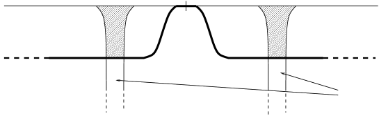
Figure 1. The contour deformation in case 3 and the support properties of the almost analytic extension of $\Psi$.

By Stokes’s formula we get exactly the same contributions as in case 1 (since near $0$, $\widetilde{\Psi}=0$) with an additional term

(5.16) $$\frac{i}{2\pi}\int_{\Omega}\bar{\partial}\widetilde{\Psi}\left(z\right)e^{-itz}\chi{(R(z)}{(z^{2}+i)^{-L}}\chi\,dz$$

where $\Omega$ is the support of $\bar{\partial}\widetilde{\Psi}$ between the real axis and the new contour (shaded in Fig. 1). Since $\bar{\partial}\widetilde{\Psi}\left(z\right)={\mathcal{O}}\left(|\mathop{\rm Im}\nolimits z|^{\infty}\right)$, a repeated integration by parts shows that this last term is ${\mathcal{O}}\left(t^{-\infty}\right)$ (in the energy norm). ∎

Proof of Corollary 3: We follow the argument of Burq [6]. The left hand side of (5.13) is bounded by the same quantity at $t=0$, and in particular by $\|u_{0}\|_{H^{1}}^{2}+\|u_{1}\|_{L^{2}}^{2}$. The estimate (5.13) shows that, in case 1 (that is, the case considered in Corollary 3), it is also bounded by $e^{-\alpha t}\|u_{0}\|_{H^{K+1}}+\|u_{1}\|_{H^{K}}$. Interpolation between these two estimates gives (1.2).      

Erratum to “Resolvent estimates for normally hyperbolic trapped sets”, Ann. Inst. Henri Poincaré (A), 12(7)(2011), 1349-1385.

In this erratum we correct three errors in the recent paper “Resolvent estimates for normally hyperbolic trapped sets”, Ann. Inst. Henri Poincaré (A), 12(7)(2011), 1349-1385. The errors are minor and do not affect the correctness of the principal results (although one mild hypothesis needs to be explicitly added). Descriptions of these errors and the necessary corrections are as follows. Note that this is the second revision of this erratum, now reflecting the addition of an explicit hypothesis that the trapped set should be symplectic.

• In §3.5 we omitted a crucial condition on $G$ which is needed to have (3.24). In (3.20) we need to strengthen the second condition to

  $$G=G_{1}+\log(1/h)G_{2},\ \ \partial^{\alpha}H_{p}^{k}G_{1}={\mathcal{O}}((h/\tilde{h})^{-|\alpha|/2}),\ \ k+|\alpha|\geq 1,\ \ \partial^{\alpha}G_{2}={\mathcal{O}}(1).$$

  This is satisfied for the weight $G$ in §§4.2–4.3. Expression (3.24) holds for $\ell\geq 2,$ while the case $\ell=1$ yields the slight variant:

  $$\operatorname{ad}_{G^{w}(x,hD)}P\in h\log(1/h)\widetilde{\Psi}_{1/2}.$$

  The analysis follows from [5, §8.2] and is the same as in [2, §8]. See also [1, §7] and [4, Proposition 4.2] for similar arguments.

• Lemma 4.1 is incorrect as stated. The conclusion (4.4) does not hold for any defining functions of $\Gamma_{\pm}$ as can be seen by multiplying $\varphi_{\pm}$ by $e^{f}$ and having $|H_{f}|$ large somewhere. We are grateful to Semyon Dyatlov for pointing this out.

  The error in the proof comes from the fact that $C$ in the second displayed formula there may be greater than $1$.

  The simple correction is to state that there exists some choice of defining functions satisfying (4.4) in some neighbourhood of $K$. We start with given defining functions $\tilde{\varphi}_{\pm}$ and then, similarly as in [2, Proof of Proposition 7.4] (but for defining functions rather than their squares as in [2]), set

  $${\widehat{\varphi}}_{\pm}(\rho)\stackrel{{\scriptstyle\rm{def}}}{{=}}\int_{0}^{T}\tilde{\varphi}_{\pm}(\exp tH_{p}(\rho))\,dt.$$

  These are defining functions of $\Gamma_{\pm}$ as these sets are invariant under the flow.

  Then

  $$H_{p}{\widehat{\varphi}}_{\pm}(\rho)=\tilde{\varphi}_{\pm}(\exp TH_{p}(\rho))-\tilde{\varphi}_{\pm}(\rho).$$

  Since $|\tilde{\varphi}_{\pm}(\rho)|\sim d(\rho,\Gamma_{\pm})$, the second displayed formula in the proof of Lemma 4.1 with $T$ large enough (for $\rho$ in a $T$ dependent neighbourhood of $K$), shows that

  $$|\tilde{\varphi}_{+}(\exp TH_{p}(\rho))|\ll|\tilde{\varphi}_{+}(\rho)|,\ \ |\tilde{\varphi}_{-}(\rho)|\ll|\tilde{\varphi}_{-}(\exp TH_{p}(\rho))|.$$

  Hence

  $$H_{p}{\widehat{\varphi}}_{+}(\rho)\sim-\tilde{\varphi}_{+}(\rho)\sim-{\widehat{\varphi}}_{+}(\rho),\ \ H_{p}{\widehat{\varphi}}_{-}(\rho)\sim\tilde{\varphi}_{-}(\exp TH_{p}(\rho))\sim{\widehat{\varphi}}_{-}(\rho),$$

  with constants depending on $T$. This gives (4.4).

• The assertion, in Dynamical Hypothesis (2), that $K$ must automatically be symplectic, seems to be false. We must therefore add the hypothesis that $K$ is symplectic, as this fact is used crucially in the end of the proof of Lemma 4.1, where we observe that $\{\varphi_{+},\varphi_{-}\}\neq 0.$ We are grateful to Semyon Dyatlov for pointing this out.

References

- [1] I. Alexandrova, J.-F. Bony, and T. Ramond, Semiclassical scattering amplitude at the maximum of the potential, Asymptotic Analysis, 58(2008), 57–125.
- [2] A.V. Bolsinov, S.V. Matveev, and A.T. Fomenko, Topological classification of integrable Hamiltonian systems with two degrees of freedom. List of all systems of small complexity, Russ. Math. Surv., 45 (1990), No. 2, 59-99.
- [3] J.-F. Bony and D. Häfner, Decay and non-Decay of the local energy for the wave equation on the De Sitter-Schwarzschild metric, Comm. Math. Phys. 282(2008), 697-719.
- [4] J.-F. Bony, S. Fujiie, T. Ramond, and M. Zerzeri, Spectral projection, residue of the scattering amplitude, and Schrodinger group expansion for barrier-top resonances, arXiv:0908.3444
- [5] J.-M. Bony and J.-Y. Chemin, Espaces fonctionnels associés au calcul de Weyl-Hörmander, Bull. Soc. math. France, 122(1994), 77-118.
- [6] N. Burq, Smoothing effect for Schrödinger boundary value problems, Duke Math. J. 123(2004), 403–427.
- [7] N. Burq, C. Guillarmou, and A. Hassell, Strichartz estimates without loss on manifolds with hyperbolic trapped geodesics, , Geom. Funct. Anal. 20 (2010), no. 3, 627–656.
- [8] P. Blue and J. Sterbenz, Uniform decay of local energy and the semi-linear wave equation on Schwarzschild space, Comm. Math. Phys. 268 (2006), no. 2, 481–504.
- [9] N. Burq and M. Zworski, Resonance expansions in semi-classical propagation, Comm. Math. Phys. 232(2001), 1–12.
- [10] N. Burq and M. Zworski, Control in the presence of a black box, J. Amer. Math. Soc. 17(2004), 443–471.
- [11] B. Carter, Global structure of the Kerr family of gravitational Fields, Phys. Rev. 174(1968), 1559–1571.
- [12] H. Christianson, Semiclassical non-concentration near hyperbolic orbits, J. Funct. Anal. 262 (2007), 145–19.
- [13] H. Christianson, Quantum monodromy and non-concentration near a closed semi-hyperbolic orbit, arXiv:0803.0697, to appear in Trans. Amer. Math. Soc.
- [14] M. Dafermos and I. Rodnianski, Lectures on black holes and linear waves, arXiv:0811.0354v1.
- [15] K. Datchev, Local smoothing for scattering manifolds with hyperbolic trapped sets, Comm. Math. Phys. 286(3)(2009), 837–850.
- [16] M. Dimassi and J. Sjöstrand, Spectral Asymptotics in the semiclassical limit, Cambridge University Press, 1999.
- [17] R. Donninger, W. Schlag, and A. Soffer, A proof of Price’s Law on Schwarzschild black hole manifolds for all angular momenta, arXiv:0908.4292
- [18] R. Donninger, W. Schlag, and A. Soffer, On pointwise decay of linear waves on a Schwarzschild black hole background, arXiv:0911.3179
- [19] S. Dyatlov, Quasinormal modes for Kerr-De Sitter black holes: a rigorous definition and the behaviour near zero energy.
-
[20]
L.C. Evans and M. Zworski, Lectures on semiclassical
analysis,
http://math.berkeley.edu/zworski/semiclassical.pdf - [21] N. Fenichel, Persistence and smoothness of invariant manifolds for flow, Indiana Univ. Math. J. 21 No. 3 (1972), 193–226.
- [22] F. Finster, N. Kamran, J. Smoller, and S.-T. Yau. Decay of solutions of the wave equation in the Kerr geometry. Comm. Math. Phys., 264(2):465–503, 2006.
- [23] F. Finster, N. Kamran, J. Smoller, and S.-T. Yau. Erratum: “Decay of solutions of the wave equation in the Kerr geometry” [Comm. Math. Phys. 264 (2006), no. 2, 465–503]. Comm. Math. Phys., 280(2):563–573, 2008.
- [24] B. Helffer, J. Sjöstrand, Résonances en limite semi-classique, Mém. Soc. Math. France (N.S.) 24–25(1986),
- [25] C. Gérard and J. Sjöstrand, Semiclassical resonances generated by a closed trajectory of hyperbolic type, Comm. Math. Phys. 108 (1987), 391-421.
- [26] C. Gérard and J. Sjöstrand, Resonances en limite semiclassique et exposants de Lyapunov, Comm. Math. Phys. 116 (1988), 193-213.
- [27] L. Hörmander, The Analysis of Linear Partial Differential Operators, Vol. III,IV, Springer-Verlag, Berlin, 1985.
- [28] M.W. Hirsch, C.C. Pugh and M. Shub, Invariant manifolds Lecture Notes in Mathematics, Vol. 583. Springer-Verlag, Berlin-New York, 1977.
- [29] M. Ikawa, Decay of solutions of the wave equation in the exterior of several convex bodies, Ann. Inst. Fourier, 38(1988), 113-146.
- [30] K.D. Kokkotas and B.G. Schmidt, Quasi-normal modes of stars and black holes, Living Rev. Relativ. 2, 2 (1999), arXiv:9909058
- [31] S. Nonnenmacher and M. Zworski, Quantum decay rates in chaotic scattering, Acta Mathematica 203(2009), 149-233.
- [32] S. Nonnenmacher and M. Zworski, Semiclassical resolvent estimates in chaotic scattering, Applied Mathematics Research eXpress 2009; doi: 10.1093/amrx/abp003.
- [33] V. Petkov and L. Stoyanov, Analytic continuation of the resolvent of the Laplacian and the dynamical zeta function, Anal. PDE 3 (2010), no. 4, 427–489.
- [34] A. Sá Barreto and M. Zworski Distribution of resonances for spherical black holes, Math. Res. Lett. 4 (1997), no. 1, 103–121.
- [35] J. Sjöstrand, Geometric bounds on the density of resonances for semiclassical problems, Duke Math. J., 60(1990), 1–57
- [36] J. Sjöstrand, A trace formula and review of some estimates for resonances, in Microlocal analysis and spectral theory (Lucca, 1996), 377–437, NATO Adv. Sci. Inst. Ser. C Math. Phys. Sci., 490, Kluwer Acad. Publ., Dordrecht, 1997.
- [37] J. Sjöstrand and M. Zworski, Complex scaling and the distribution of scattering poles, Journal of A.M.S., 4(4)(1991), 729-769
- [38] J. Sjöstrand and M. Zworski, Quantum monodromy and semiclassical trace formulae, J. Math. Pure Appl. 81(2002), 1–33.
- [39] J. Sjöstrand and M. Zworski, Fractal upper bounds on the density of semiclassical, Duke Math. J., P137(2007), 381–459.
- [40] P. Stefanov, Approximating resonances with the complex absorbing potential method. Comm. Partial Differential Equations, 30(10-12):1843–1862, 2005.
- [41] S.H. Tang and M. Zworski, Resonance expansions of scattered waves, Comm. Pure Appl. Math. 53(2000), 1305–1334.
- [42] D. Tataru and M. Tohaneanu, Local energy estimate on kerr black hole backgrounds, preprint, 2008, arXiv:0810.5766.
- [43] M. Tohaneanu, Strichartz estimates on Kerr black hole backgrounds, arXiv:0910.1545
- [44] J. Wunsch and M. Zworski, Distribution of resonances for asymptotically euclidean manifolds, J. Diff. Geometry. 55(2000), 43–82.
- [45] M. Zworski, Poisson formula for resonances in even dimensions, Asian J. Math. 2(1998), 615–624.
- [46] M. Zworski, Resonances in Physics and Geometry, Notices of the AMS, 46 no.3, March, 1999.

References

-
[1]
K. Datchev and S. Dyatlov,
Fractal Weyl laws for asymptotically hyperbolic manifolds,
arXiv:1206.2255 - [2] J. Sjöstrand and M. Zworski, Fractal upper bounds on the density of semiclassical resonances, Duke Math. J., P137(2007), 381–459.
- [3] Jared Wunsch and Maciej Zworski, Resolvent estimates for normally hyperbolic trapped sets, Ann. Henri Poincaré, 12(7):1349–1385, 2011.
- [4] M. Zworski, Fractal Weyl laws for quantum resonances, Talk at Ecole Polytechnique, Novembre 2004, http://math.berkeley.edu/ zworski/talkX.ps
- [5] M. Zworski, Semiclassical Analysis, Graduate Studies in Mathematics 138, AMS 2012.