Nonabelian Bosonic Currents in Cosmic Strings

Abstract

A nonabelian generalization of the neutral Witten current-carrying string model is discussed in which the bosonic current-carrier belongs to a two dimensional representation of SU(2). We find that the current-carrying solutions can be of three different kinds: either the current spans a U(1) subgroup, and in which case one is left with an abelian current-carrying string, or the three currents are all lightlike, travelling in the same direction (only left or right movers). The third, genuinely nonabelian situation, cannot be handled within a cylindrically symmetric framework, but can be shown to depend on all possible string Lorentz invariant quantities that can be constructed out of the phase gradients.

I Introduction

Topological cosmic strings or superstrings of cosmological size are one-dimensional extended objects which are believed to have been formed in the early phases of cosmological evolution. They are of considerable interest because they may offer a observable window on the high energy physics of the primordial universe, i.e., at grand unified scales.

Topological strings are produced in phase transitions associated with spontaneous symmetry breaking. This is the standard Kibble mechanism Kibble (1976, 1980). Almost all supersymmetric grand unified theories in which hybrid inflation Linde (1994); Copeland et al. (1994); Dvali et al. (1994) can be realized lead to the formation of topological strings Jeannerot (1996, 1997); Jeannerot et al. (2003a, b). Besides, most classes of superstring compactification lead to a spontaneous breaking of a pseudo-anomalous U$(1)$ gauge symmetry producing local cosmic strings Binétruy et al. (1998). Such strings also form in the case where the Higgs field has a non-minimal kinetic term Babichev et al. (2009).

The simplest kind of topological string is the Nambu-Goto string which is described by the Nambu-Goto action Gotō (1971); Nambu (1974). The Nambu-Goto action is the worldsheet formulation counterpart of a field theory description in which the string arises as a solitonic solution of the abelian Higgs model Nielsen and Olesen (1973). Such a string has no internal structure and is described entirely in terms of a worldsheet Lagrangian and the tension per unit length of the string.

Most observational signatures in the gravitational sector expected from topological strings have been derived and simulated numerically for Nambu-Goto strings. There are five main possible observational effects (see Shellard and Vilenkin (1994); Peter and Uzan (2009) and references therein): beamed gravitational wave bursts from kinks and particle acceleration; deflection, gravitational lensing effects and multiple image effects; Doppler shifting effects; background gravitational radiation from string loops; and string effects in the cosmic microwave background. The existence of kinks along the strings has been shown to occur also for current-carrying strings Cordero-Cid et al. (2002) and the electromagnetic effects of such strings, which are absent in the simpler Nambu-Goto string, have been investigated. An especially interesting observational consequence of the presence of cosmic string networks in the early universe potentially because it is susceptible to be detected in the cosmic microwave background is the Gott-Kaiser-Stebbins effect Gott (1985); Kaiser and Stebbins (1984). This effect consists in a temperature shift that is due to the gravitational lensing of photons passing near a moving source.

Cosmic superstrings are formed by tachyon condensation at the end of brane inflation Sarangi and Tye (2002); Jones et al. (2003). The tachyons are complex scalars [with a local U(1) gauge symmetry] identifiable with the ground state open string modes of the Neveu-Schwarz sector that end on coincident non-BPS branes and antibranes Green (1994); Banks and Susskind (1995); Green and Gutperle (1996); Lifschytz (1996). There exist associated gauge fields living on the brane and antibrane so that there exists a U(1)$\times$U(1) symmetry on the brane-antibrane configuration. A first linear combination of the U(1)’s is higgsed Dvali and Vilenkin (2003, 2004) leading to the appearance of a first kind of cosmic superstrings that are D $p$-branes with $p-1$ dimensions compactified Majumdar and Davis (2002). In type IIB superstring theory, and given a spacetime manifold $\mathcal{M}$, such stable $p$-branes, can, for example, be obtained by considering a $p+2$ brane-antibrane pair stretching over a submanifold $\mathbbm{R}^{p+3}\subset\mathcal{M}$. The $p+2$ brane-antibrane pair will annihilate unless a topological obstruction exists. This obstruction can be obtained from K-theory Sen (1998); Witten (1998); Olsen and Szabo (1999). A second linear combination of the U(1)’s leads to the formation of F-strings Dvali and Vilenkin (2003, 2004).

All these types of strings have until recently been considered as structureless, so their dynamics is given by the Nambu-Goto action. Numerical simulations of networks (see Fraisse et al. (2008) and references therein) of such strings have been produced with the result of scaling, a property thanks to which the string network never comes to dominate the Universe evolution, but neither are the string completely washed out of the Universe, so their effect, however small, is still detectable.

The Nambu-Goto string can be generalized to the case of a string with internal structure. Such a string can be obtained by including a coupling of the string forming Higgs field to additional (bosonic or fermionic, with global or local, abelian, or nonabelian symmetry) fields in the theory. In part of the parameter space, these fields condense onto the string (the symmetry gets broken) leading to the appearance of currents on the worldsheet in the form of Goldstone bosons propagating along string Witten (1985). In such a case, the current-carrying string can be described using a worldsheet Lagrangian and a nontrivial equation of state relating the tension per unit length to the energy density of the string Carter (1989a, b, 1990a, 1992); the actual form of this equation of state was discussed numerically Peter (1992a, b, 1993a) and analytically Carter and Peter (1995). The presence of currents on the worldsheet modifies only slightly the gravitational properties of the long strings Peter and Puy (1993); Garriga and Peter (1994), but it also halts cosmic string loop decay caused by dissipative effects, thereby yielding new equilibrium configurations Martin and Peter (2000); Cordero-Cid et al. (2002) named vortons Davis and Shellard (1988a, b, 1989); Carter (1991, 1990b, 1995). Those can potentially change drastically the cosmological network evolution, at the point of ruling such strings out.

Although the current-carrying property of cosmic strings is in fact fairly generic Peter (1992c); Davis and Peter (1995); Peter et al. (2003), a possibility that has, until now, been completely disregarded is that for which the string would be endowed not only with many currents Lilley et al. (2009), but also with currents of a nonabelian kind, as is to be expected in most grand unified theories. This natural extension of the Witten idea leads to numerous new difficulties, as in particular the internal degrees of freedom manifold is intrinsically curved, so that a local, flat, description of the string worldsheet manifold, turns out to be inappropriate Carter (2010a, b). This paper is devoted to the specific task of obtaining the equivalent microscopic structure of a nonabelian current-carrying cosmic string.

To do so, we restrict attention to the global situation in which, in a way similar to the so-called neutral Witten model Peter (1992a), we wish to capture the essential internal dynamics of the string without the undue complication of adding extra gauge vector fields. In the case of an abelian current, it was indeed shown that these contributions, although of potential great cosmological relevance (see, e.g. Ref. Peter (1993b) and references therein), can however be treated in a perturbative way, not modifying in any essential way the actual microscopic structure Peter (1992b). We therefore assume, as a toy model, a U$(1)$ Higgs model whose breaking leads to the existence of the strings themselves, coupled to an SU$(2)$ doublet through a scalar potential with parameters ensuring a condensate. We first describe the fields and notation, derive their dynamical equations in full generality, and then discuss the condensate configuration. After having recovered the abelian cases as particular solutions of the general nonabelian situation, we concentrate on the strictly nonabelian solutions. We obtain an exact configuration, called trichiral, and show how this model makes explicit the obstruction theorem first obtained by Carter Carter (2010a, b). We then derive the stress energy tensor and its eigenvalues, namely the energy per unit length and tension, and show that they depend on all the possible two-dimensional Lorentz invariants that can be constructed from the phase gradients (and second derivatives) of the angular variables in the internal space. We conclude by discussing the possible cosmological consequences of this new category of objects.

II Fields content

The simplest nonabelian current-carrying string model that can be written down is that in which a U$(1)$ symmetry is spontaneously broken by means of a scalar complex Higgs field $\phi$, itself coupled to $\bm{\Sigma}$, a scalar field belonging to an arbitrary representation of a nonabelian group $G$. The string-forming action stems from the Higgs Lagrangian

$$\mathcal{L}_{{}_{\mathrm{S}}}=-D_{\mu}{\phi}^{\star}D^{\mu}{\phi}-\frac{1}{4}C_{\mu\nu}C^{\mu\nu}-V_{{}_{\mathrm{H}}}\left(\phi\right),$$ (1)

where

$$C_{\mu\nu}=\nabla_{\mu}C_{\nu}-\nabla_{\nu}C_{\mu}$$ (2)

and the U$(1)$ covariant derivative is expressed in terms of the U$(1)$ gauge field $C_{\mu}$ as

$$D_{\mu}\phi=\nabla_{\mu}\phi+iqC_{\mu}\phi,$$ (3)

where $q$ is the charge. $V_{{}_{\mathrm{H}}}$ can be chosen without lack of generality as the Higgs symmetry breaking potential, namely

$$V_{{}_{\mathrm{H}}}=\displaystyle\frac{\lambda_{\phi}}{4}\left(\left|\phi\right|^{2}-\eta^{2}\right)^{2},$$ (4)

with $\lambda_{\phi}$ a coupling constant and $\eta$ the Higgs vacuum expectation constant (vev) at infinity.

The current part of the Lagrangian reads

$$\mathcal{L}_{{}_{\mathrm{C}}}=-\left(\partial_{\mu}{\bm{\Sigma}}\right)^{\dagger}\cdot\partial^{\mu}\bm{\Sigma}-V_{{}_{\mathrm{C}}}\left(\bm{\Sigma}\right),$$ (5)

where $\bm{\Sigma}$ transforms according to a yet arbitrary representation of the global invariance group whose structure constants we write as $f^{a}_{\ bc}$; these are defined through the commutation relations for $\{T^{a}\}$, the algebra of $G$, namely

$$\left[T^{a},T^{b}\right]=if^{c}_{\ ab}T_{c}.$$ (6)

In Eq. (6) and in the following, the group indices are denoted by latin smallcap letters $a,b,\cdots=1,\cdots,N$ which run to $N$, the group dimension. The potential appearing in the current action is the self-interacting potential chosen as

$$V_{{}_{\mathrm{C}}}\left(\bm{\Sigma}\right)=\pm m_{\sigma}^{2}\bm{\Sigma}^{\dagger}\cdot\bm{\Sigma}+\lambda_{\sigma}\left(\bm{\Sigma}^{\dagger}\cdot\bm{\Sigma}\right)^{2},$$ (7)

thus introducing the vacuum mass and self-interaction constants $m_{\sigma}$ and $\lambda_{\sigma}$. In Eq. (7), we have introduced a sign parameter which accounts for the possibility that SU$(2)$ is broken ($-$) or unbroken ($+$) far from the string core. The first possibility is usually not taken into account when one considers the Witten model since in that case, one has in mind that the condensate depicts electromagnetism, which is obviously unbroken far from the string. In the nonabelian case however, it is reasonable to assume a broken symmetry far from the string as well, in particular if one is to identify this symmetry with that of the electroweak phenomenology.

The total action of the system can be written as

$${\cal L}={\cal L}_{{}_{\mathrm{S}}}+{\cal L}_{{}_{\mathrm{C}}}-V_{\mathrm{int}}\,,$$ (8)

where the interaction term couples the two scalar fields $V_{\mathrm{int}}\left(\phi,\bm{\Sigma}\right)$. This potential, again for illustrative purposes below, shall be taken as the most general renormalizable one, namely

$$V_{\mathrm{int}}\left(\phi,\bm{\Sigma}\right)=f\left(\left|\phi\right|^{2}-\eta^{2}\right)\bm{\Sigma}^{\dagger}\cdot\bm{\Sigma},$$ (9)

with a positive coupling constant $f$ to ensure vacuum stability. The vacuum far from the string therefore depends on the representation $\bm{\Sigma}$ belongs to. The microscopic parameters that allow for a condensate to form are similar to those of the abelian current case; they have been discussed in particular in Ref. Peter (1992a).

III Field equations

Having specified the field content and the action of the system, one can now derive the corresponding equations of motion. The equations of motion of the system consisting of the string-forming fields $\phi$ and $C_{\mu}$ and the current carrier $\bm{\Sigma}$ are

$$\nabla_{\mu}\nabla^{\mu}\phi+2iqC^{\mu}\nabla_{\mu}\phi+iq\phi\nabla_{\mu}C^{\mu}-q^{2}C^{\mu}C_{\mu}\phi-\frac{\partial V}{\partial\phi^{*}}=0,$$ (10)

for the string-forming Higgs field,

$$\nabla_{\mu}C^{\mu\nu}-iq(\phi\nabla^{\nu}\phi^{*}-\phi^{*}\nabla^{\nu}\phi)-2q^{2}C^{\nu}|\phi|^{2}=0$$ (11)

for the associated U$(1)$ gauge field, and

$$\kern 1.0pt\vbox{\hrule height=1.2pt\hbox{\vrule width=1.2pt\hskip 3.0pt\vbox{\vskip 6.0pt}\hskip 3.0pt\vrule width=0.6pt}\hrule height=0.6pt}\kern 1.0pt\bm{\Sigma}=\frac{\partial V}{\partial\bm{\Sigma}^{\dagger}}$$ (12)

for the current carrier.

The energy-momentum tensor of the system is given by the usual relation

$$T_{\mu\nu}\equiv g_{\mu\nu}{\mathcal{L}}-2\frac{\delta\mathcal{L}}{\delta g^{\mu\nu}},$$ (13)

and can be decomposed into a scalar and a vector part, namely

$$T_{\mu\nu}=T^{\mathrm{s}}_{\mu\nu}+T^{\mathrm{v}}_{\mu\nu},$$ (14)

where

$$T^{\mathrm{s}}_{\mu\nu} = D_{(\mu}\phi^{*}D_{\nu)}\phi-g_{\mu\nu}D_{\gamma}\phi^{*}D^{\gamma}\phi$$ (15)

$$+\partial_{(\mu}\bm{\Sigma}^{\dagger}\cdot\partial_{\nu)}\bm{\Sigma}-g_{\mu\nu}\left(\partial_{\gamma}\bm{\Sigma}\right)^{\dagger}\cdot\partial^{\gamma}\bm{\Sigma}$$

$$-g_{\mu\nu}V\left(\phi,\bm{\Sigma}\right),$$

with parentheses denoting symmetrization of the indices, i.e., $S_{(\alpha\beta)}\equiv S_{\alpha\beta}+S_{\beta\alpha}$, and

$$T^{\mathrm{v}}_{\mu\nu}=-\left(F_{\mu\alpha}F^{\alpha}_{\ \nu}+\frac{1}{4}g_{\mu\nu}F_{\alpha\beta}F^{\alpha\beta}\right)\,,$$ (16)

where we have defined $F_{\alpha\beta}\equiv\partial_{\alpha}C_{\beta}-\partial_{\beta}C_{\alpha}$.

From this stress-energy tensor and the field equations, we shall now derive the full microscopic structure of the system.

IV The condensate

Having derived the most general form of the equations of motion, we now turn to the specific situation where an straight, infinitely long, cosmic string is present. A typical vortex solution aligned along the $z$ axis in polar coordinates $r$ and $\theta$ is then given by the Nielsen-Olesen ansatz

$$\phi=\varphi(r)\mbox{e}^{in\theta}\ \ \ \hbox{and}\ \ \ C_{\mu}=C_{\theta}(r)\delta_{\mu}^{\theta},$$ (17)

where $n\in\mathbb{Z}$. Although the specific form of the potential is irrelevant for most of what follows, the shape (4), being the most general renormalizable function satisfying this constraint, is used in the numerical illustrations below. Inserting the above ansatz into the equations of motion, Eq. (10) takes the form

$$\frac{\mbox{d}^{2}\varphi}{\mbox{d}r^{2}}+\frac{1}{r}\frac{\mbox{d}\varphi}{\mbox{d}r}=\frac{Q^{2}}{r^{2}}\varphi+\frac{\partial V}{\partial\varphi},$$ (18)

while Eq. (11) becomes

$$\frac{\mbox{d}^{2}Q}{\mbox{d}r^{2}}-\frac{1}{r}\frac{\mbox{d}Q}{\mbox{d}r}=2q^{2}Q\varphi^{2},$$ (19)

where we have defined $Q\equiv n+qC_{\theta}$. In Eq. (18), the last term of the r.h.s involves not only the derivative of the self-interaction potential $V_{{}_{\mathrm{H}}}$, but also that of the coupling term $V_{\mathrm{int}}$, so that this equation also depends on the SU$(2)$ doublet amplitude. It is through this “backreaction” term that the string itself is affected by the presence of the current.

Let us now discuss in more detail the form of the current-carrier scalar field $\bm{\Sigma}$. Our goal is to find the most general ansatz for $\bm{\Sigma}$ in cylindrical coordinates. The case where $G=\mathrm{U}(1)$ represents the usual so-called superconducting string model originally introduced by Witten Witten (1985). In this particular case, $\Sigma$ is a complex field vanishing in vacuum, i.e. far from the string. Its coupling with the string-forming Higgs field yields an instability in the vortex core leading to a condensate: far from the string, in vacuum, where the Higgs field is equal to its vev $|\phi|=\eta$, the interaction term $V_{\mathrm{int}}$ vanishes so that $\Sigma$ must vanish. The string location, defined as the set of points where $\phi=0$, however, is no longer vacuum-like from the point of view of $\Sigma$, and indeed the parameters of the potential (9) can be chosen Peter (1992a, b) such that $\Sigma$ does not vanish inside the vortex.

One can pick a specific gauge in which $\Sigma$ is real, $\Sigma=\sigma(r)$ say, depending only on the distance to the string, with $\sigma\in\mathbb{R}$ and $\lim_{r\to\infty}\sigma(r)=0$, and generate all the solutions by applying a gauge transformation, in this case a phase. The full solution then reads

$$\Sigma=\mbox{e}^{i\psi(z,t)T}\sigma(r),$$ (20)

where the phase transformation can now depend on the worldsheet internal coordinates and we did not take into account a possible dependence in the external coordinates. In Eq. (20), we have written explicitly the generator of the U(1) translation as $T$, even though it is not necessary in this simplifying case for which the scalar field is a mere singlet under this extra U(1); note that this could be different if $\Sigma$ were belonging to the representation of a larger group containing this U(1).

Written in the form (20) with the generator, the solution is easily generalizable to the nonabelian case. We again choose a gauge in which $\bm{\Sigma}=\bm{\sigma}(x^{\perp})$, with $\bm{\sigma}$ in the desired representation but depending only on the external coordinates $x^{\perp}$ (in practice the radial distance $r$), and produce the full solution by exponentiation of the generators $T_{a}$ as

$$\bm{\Sigma}=\mbox{e}^{i\psi^{a}\left(\xi\right)T_{a}}\bm{\sigma}(x^{\perp}),$$ (21)

where the functions $\psi_{a}$ a priori depend on the internal coordinates $\xi$ only. As it turns out however Carter (2010a, b), in the more general case of a nonabelian symmetry, the fields $\psi_{a}$ live on a curved manifold which cannot, in general, be smoothly projected on the flat manifold describing the string worldsheet. As a result, one must assume that the fields $\psi_{a}$ depend on all embedding coordinates.

The form (21) is not, unfortunately, directly usable, as the derivative of the group element is not easy to handle. Indeed, for a noncommuting algebra, one has

$$\partial_{\mu}U=i\partial_{\mu}\bm{\psi}\cdot\int_{0}^{1}U(1-p)\bm{T}U(p)\mbox{d}p\not=i\partial_{\mu}\bm{\psi}\cdot\bm{T}U,$$ (22)

where $U(p)\equiv\exp(ip\bm{\psi}\cdot\bm{T})$ and $U\equiv\exp(i\bm{\psi}\cdot\bm{T})=U(1)$ and, the last relation becoming an equality in the abelian case. Restricting attention to SU(2) however, allows simple calculations to be carried out completely since one then has the useful relation

$$\mbox{e}^{i\alpha\bm{n}\cdot\bm{\tau}}=\cos\alpha\mathbb{1}+i\bm{n}\cdot\bm{\tau}\sin\alpha,\ \ \ \hbox{with}\ \ \ n_{a}n^{a}=1,$$ (23)

between the Pauli matrices $\tau^{a}$, generators of SU(2), and their exponentiated form. We therefore restrict attention to a scalar field belonging to the representation $\bm{2}$ of SU(2), i.e. a doublet, and thus assume in what follows that the current-carrier takes the form

$$\bm{\Sigma}=\left(\cos\alpha\mathbb{1}+i\bm{n}\cdot\bm{\tau}\sin\alpha\right)\sigma g,\ \ \ \ \hbox{with}\ \ \ g\equiv\frac{1}{\sqrt{2}}\left(\begin{array}[]{c}0\cr 1\end{array}\right).$$ (24)

Notice that Eq. (18), together with the assumption of a potential depending only on the amplitude $\bm{\Sigma}^{\dagger}\cdot\bm{\Sigma}=\frac{1}{2}\sigma^{2}$, shows that $\sigma=\sigma(r)$ only. But, as already mentioned above, the angle $\alpha$ and the normalized vector $n^{a}$ a priori depend on all the coordinates.

With the form (24) for the scalar field, the variation of the potential is

$$\frac{\partial V}{\partial\bm{\Sigma}^{\dagger}}=\frac{1}{2}\frac{\partial V}{\partial\sigma}\left(\cos\alpha\mathbb{1}+i\bm{n}\cdot\bm{\tau}\sin\alpha\right)g,$$ (25)

which provides the equation of motion through Eq. (12). Indeed, projecting this equation of motion on the identity of SU(2) yields

$$\Delta\sigma-\left[\left(\partial\alpha\right)^{2}+\tan\alpha\kern 1.0pt\vbox{\hrule height=1.2pt\hbox{\vrule width=1.2pt\hskip 3.0pt\vbox{\vskip 6.0pt}\hskip 3.0pt\vrule width=0.6pt}\hrule height=0.6pt}\kern 1.0pt\alpha\right]\sigma-2\tan\alpha\partial\alpha\cdot\partial\sigma=\frac{1}{2}\frac{\partial V}{\partial\sigma},$$ (26)

while the projection on the Pauli matrices $\tau^{a}$ leads to

$$n^{a}\left\{\Delta\sigma+\left[\frac{\kern 1.0pt\vbox{\hrule height=1.2pt\hbox{\vrule width=1.2pt\hskip 3.0pt\vbox{\vskip 6.0pt}\hskip 3.0pt\vrule width=0.6pt}\hrule height=0.6pt}\kern 1.0pt\alpha}{\tan\alpha}-\left(\partial\alpha\right)^{2}\right]\sigma+2\frac{\partial\alpha\cdot\partial\sigma}{\tan\alpha}\right\}+2\left(\partial\sigma+\frac{\sigma\partial\alpha}{\tan\alpha}\right)\cdot\partial n^{a}+\sigma\kern 1.0pt\vbox{\hrule height=1.2pt\hbox{\vrule width=1.2pt\hskip 3.0pt\vbox{\vskip 6.0pt}\hskip 3.0pt\vrule width=0.6pt}\hrule height=0.6pt}\kern 1.0ptn^{a}=\frac{1}{2}\frac{\partial V}{\partial\sigma}n^{a},$$ (27)

which in turn implies, upon projection on $n_{a}$, recalling this vector to be normalized to unity, that

$$\Delta\sigma-\left[\left(\partial\alpha\right)^{2}-\frac{\kern 1.0pt\vbox{\hrule height=1.2pt\hbox{\vrule width=1.2pt\hskip 3.0pt\vbox{\vskip 6.0pt}\hskip 3.0pt\vrule width=0.6pt}\hrule height=0.6pt}\kern 1.0pt\alpha}{\tan\alpha}-n_{a}\kern 1.0pt\vbox{\hrule height=1.2pt\hbox{\vrule width=1.2pt\hskip 3.0pt\vbox{\vskip 6.0pt}\hskip 3.0pt\vrule width=0.6pt}\hrule height=0.6pt}\kern 1.0ptn^{a}\right]\sigma+2\frac{\partial\alpha\cdot\partial\sigma}{\tan\alpha}=\frac{1}{2}\frac{\partial V}{\partial\sigma}.$$ (28)

This last equation can be used in order to simplify Eq. (27). Indeed, inserting Eq. (28) into Eq. (27), one obtains

$$\kern 1.0pt\vbox{\hrule height=1.2pt\hbox{\vrule width=1.2pt\hskip 3.0pt\vbox{\vskip 6.0pt}\hskip 3.0pt\vrule width=0.6pt}\hrule height=0.6pt}\kern 1.0ptn^{a}+2\left(\frac{\partial\sigma}{\sigma}+\frac{\partial\alpha}{\tan\alpha}\right)\cdot\partial n^{a}-\left(n_{b}\kern 1.0pt\vbox{\hrule height=1.2pt\hbox{\vrule width=1.2pt\hskip 3.0pt\vbox{\vskip 6.0pt}\hskip 3.0pt\vrule width=0.6pt}\hrule height=0.6pt}\kern 1.0ptn^{b}\right)n^{a}=0\,,$$ (29)

which provides a clean equation for the evolution of the vector $n^{a}$. Note also that Eqs. (26) and (28) can be combined to provide a dynamical equation for the angle $\alpha$, namely

$$\kern 1.0pt\vbox{\hrule height=1.2pt\hbox{\vrule width=1.2pt\hskip 3.0pt\vbox{\vskip 6.0pt}\hskip 3.0pt\vrule width=0.6pt}\hrule height=0.6pt}\kern 1.0pt\alpha+\frac{2}{\sigma}\partial\sigma\cdot\partial\alpha+\sin\alpha\cos\alpha\left(n_{a}\kern 1.0pt\vbox{\hrule height=1.2pt\hbox{\vrule width=1.2pt\hskip 3.0pt\vbox{\vskip 6.0pt}\hskip 3.0pt\vrule width=0.6pt}\hrule height=0.6pt}\kern 1.0ptn^{a}\right)=0,$$ (30)

and the profile of the condensate then satisfies

$$\Delta\sigma-\left[\left(\partial\alpha\right)^{2}-\left(n_{a}\kern 1.0pt\vbox{\hrule height=1.2pt\hbox{\vrule width=1.2pt\hskip 3.0pt\vbox{\vskip 6.0pt}\hskip 3.0pt\vrule width=0.6pt}\hrule height=0.6pt}\kern 1.0ptn^{a}\right)\sin^{2}\alpha\right]\sigma=\frac{1}{2}\frac{\partial V}{\partial\sigma},$$ (31)

which generalizes the abelian case by inclusion of the nonlinear term. At this stage, Eqs. (29), (30) and (31) are the equations that one needs to solve in order to determine $\sigma$, $\alpha$ and $n^{a}$.

In fact, they can still be further simplified. Indeed, let us now expand the vector components in such a way as to implement its normalization, i.e. by projecting these components on the sphere on which it evolves in terms of angular variables $\beta(t,r,z,\theta)$ and $\gamma(t,r,z,\theta)$. This gives

$$n^{1} = \sin\beta\sin\gamma,$$ (32)

$$n^{2} = \sin\beta\cos\gamma,$$ (33)

$$n^{3} = \cos\beta,$$ (34)

and therefore

$$n_{a}\kern 1.0pt\vbox{\hrule height=1.2pt\hbox{\vrule width=1.2pt\hskip 3.0pt\vbox{\vskip 6.0pt}\hskip 3.0pt\vrule width=0.6pt}\hrule height=0.6pt}\kern 1.0ptn^{a}=-\left(\partial\beta\right)^{2}-\sin^{2}\beta\left(\partial\gamma\right)^{2},$$ (35)

which shows that Eq. (30) is indeed a dynamical equation for the variable $\alpha$ only. Using the expansion (34), one can transform Eq. (29) into

$$\kern 1.0pt\vbox{\hrule height=1.2pt\hbox{\vrule width=1.2pt\hskip 3.0pt\vbox{\vskip 6.0pt}\hskip 3.0pt\vrule width=0.6pt}\hrule height=0.6pt}\kern 1.0pt\beta+2\left(\frac{\partial\sigma}{\sigma}+\frac{\partial\alpha}{\tan\alpha}\right)\cdot\partial\beta=\cos\beta\sin\beta\left(\partial\gamma\right)^{2},$$ (36)

and

$$\kern 1.0pt\vbox{\hrule height=1.2pt\hbox{\vrule width=1.2pt\hskip 3.0pt\vbox{\vskip 6.0pt}\hskip 3.0pt\vrule width=0.6pt}\hrule height=0.6pt}\kern 1.0pt\gamma+2\left(\frac{\partial\sigma}{\sigma}+\frac{\partial\alpha}{\tan\alpha}+\frac{\partial\beta}{\tan\beta}\right)\partial\gamma=0,$$ (37)

that completes a new set of dynamical equations, namely Eqs. (30), (30), (36) and (37), for the 4 independent functions $\sigma$, $\alpha$, $\beta$ and $\gamma$. A particular solution for constant angles and gradients (lowest energy state) is exemplified in Fig. 1 for the cases for which SU$(2)$ is unbroken or broken far from the string, derived using typical values for the parameters.

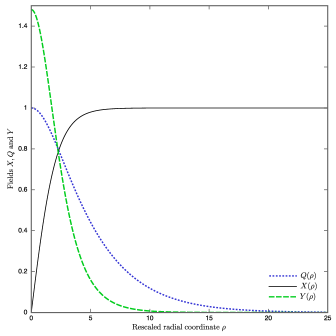
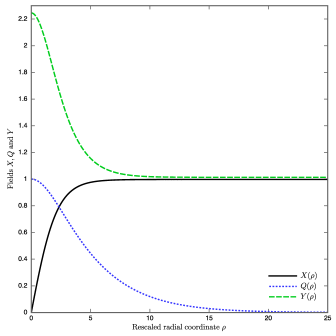
Figure 1: Typical numerical solution of the system (18), (19) and (31) with constant phases ($\alpha$, $\beta$ and $\gamma$ constant) for the dimensionless fields $X(\rho)=\varphi/\eta$, $Y(\rho)=\sigma\sqrt{\lambda_{\sigma}}/m_{\sigma}$, and $Q$ as function of the rescaled distance to the string core $\rho=\sqrt{\lambda_{\phi}}\eta r$ for parameters fixed to $\tilde{q}^{2}=0.1$, $\alpha_{1}=3.37\times 10^{-3}$, $\alpha_{2}=2.63\times 10^{-3}$, and $\alpha_{3}=5.26\times 10^{-4}$; the relevant free parameters are defined in a way reminiscent of Ref. Peter (1992a), i.e. $\tilde{q}^{2}=2q^{2}/\lambda_{\phi}$, $\alpha_{1}=m_{\sigma}^{2}/(2\lambda_{\sigma}\eta^{2})$, $\alpha_{2}=fm_{\sigma}^{2}/(2\lambda_{\phi}\lambda_{\sigma}\eta^{2})$ and $\alpha_{3}=m_{\sigma}^{4}/(2\lambda_{\phi}\lambda_{\sigma}\eta^{4})$ (the $\alpha_{i}$’s have of course nothing to do with the angle $\alpha$ introduced before). The solutions are calculated by means of Successive Over Relaxation Adler and Piran (1984) for both cases for which either the SU(2) field does not condense in vacuum, i.e. for the plus sign in front of the massive term in Eq. (7) (left panel) and that for which the SU(2) field does condense in vacuum, i.e. for the minus sign (right panel). The fact that the three curves for the Higgs field [$X(\rho)$, full line], the U(1) gauge field [$Q(\rho)$, dashed line] and the SU(2) scalar condensate [$\sigma(\rho)$, dotted line] seem to cross at a single point for the non condensing case of the left panel is purely coincidental and merely due to the specific choice of the parameters. The normalization of $Y$ with respect to that of $\sigma$ implies that in the large distance limit $\rho\to\infty$, one has $Y\to\frac{1}{2}(1-\varepsilon)$.

V abelian cases

Since the group SU$(2)$ contains invariant U$(1)$s, it can be used, restricting to special cases, to recover the abelian Witten model Witten (1985) as well as the biabelian case Lilley et al. (2009). The purpose of this section is precisely to establish the correspondences.

V.1 Witten abelian model

The form (24) for the scalar doublet can be rewritten in terms of the angles $\alpha$, $\beta$ and $\gamma$ as

$$\bm{\Sigma}=\frac{\sigma}{\sqrt{2}}\left(\begin{array}[]{c}\mbox{e}^{i\gamma}\sin\alpha\sin\beta\cr\cos\alpha-i\sin\alpha\cos\beta\end{array}\right),$$ (38)

from which one would like to single out a phase representing the U$(1)$ situation. In other words, one wants to identify real functions $\psi$, $f$ and $g$ such that

$$\bm{\Sigma}=\mbox{e}^{i\psi}\left(\begin{array}[]{c}f\cr g\end{array}\right).$$ (39)

Through identification of (39) with (38), one can easily convince oneself that there are only two possibilities, namely

$$\alpha=\beta=\frac{\pi}{2},\ \ \ \ \psi=\gamma,\ \ \ \ f=\frac{\sigma}{\sqrt{2}},\ \ \ \ g=0,$$ (40)

and

$$\psi=-\alpha,\ \ \ \beta=0,\ \ \ \ \gamma\in\mathbb{R},\ \ \ f=0,\ \ \ \ g=\frac{\sigma}{\sqrt{2}}.$$ (41)

The first case, Eq. (40), leads to $n_{a}\kern 1.0pt\vbox{\hrule height=1.2pt\hbox{\vrule width=1.2pt\hskip 3.0pt\vbox{\vskip 6.0pt}\hskip 3.0pt\vrule width=0.6pt}\hrule height=0.6pt}\kern 1.0ptn^{a}=-\left(\partial\psi\right)^{2}$, and the field equations become

$$\Delta\sigma-\left(\partial\psi\right)^{2}\sigma=\frac{1}{2}\frac{\partial V}{\partial\sigma},$$ (42)

and

$$\kern 1.0pt\vbox{\hrule height=1.2pt\hbox{\vrule width=1.2pt\hskip 3.0pt\vbox{\vskip 6.0pt}\hskip 3.0pt\vrule width=0.6pt}\hrule height=0.6pt}\kern 1.0pt\psi+\frac{2}{\sigma}\frac{\mbox{d}\sigma}{\mbox{d}r}\partial_{r}\psi=0.$$ (43)

In the abelian case, the phase does not depend on the radial distance and, hence, the last equation simply becomes $\kern 1.0pt\vbox{\hrule height=1.2pt\hbox{\vrule width=1.2pt\hskip 3.0pt\vbox{\vskip 6.0pt}\hskip 3.0pt\vrule width=0.6pt}\hrule height=0.6pt}\kern 1.0pt\psi=0$. This relation, together with Eq. (42), are exactly the equations of motion in the abelian case Witten (1985); Carter (1989a, b, 1990a, 1992); Peter (1992a, b, 1993a). The fact that we recover them from the most general framework discussed here is a consistency check of Eqs. (30), (30), (36) and (37). In the same manner, one can also check that the ansatz (41) also leads to the abelian equations of motion.

At this point, a clarification concerning the abelian situation is useful. With the set of equations above, one in principle assume the phase to vary only along the worldsheet directions, i.e., $\psi=\psi(z,t)$, see above. However, this is not merely an assumption, but rather a fact that can be demonstrated through separation of variables: since the scalar field amplitude $\sigma$ depends only on the radial distance $r$, setting $\psi=R(r)+T(\theta)+W(z,t)$, Eq. (42) tells us that

$$\left(\partial\psi\right)^{2}=\left(\frac{\mbox{d}R}{\mbox{d}r}\right)^{2}+\frac{1}{r^{2}}\left(\frac{\mbox{d}T}{\mbox{d}\theta}\right)^{2}+\left(\partial_{z}W\right)^{2}-\left(\partial_{t}W\right)^{2},$$ (44)

is a yet unknown function of $r$ only, which we write temporarily as $f(r)$. This implies that $T=T_{0}+p\theta$, and hence

$$\left(\frac{\mbox{d}R}{\mbox{d}r}\right)^{2}+\frac{p^{2}}{r^{2}}-f(r)=-\left(\partial_{z}W\right)^{2}+\left(\partial_{t}W\right)^{2}\equiv-w,$$ (45)

where $w$ is a separation constant, to be later identified with the state parameter of the abelian current-carrying cosmic string. The equation $\left(\partial_{z}W\right)^{2}-\left(\partial_{t}W\right)^{2}=w$ can also be solved trough separation of variables. Indeed, writing $W(z,t)$ as the sum of a function of $z$ and of a function of $t$, one can show that these two functions are in fact linear in $z$ and $t$ respectively.

Similarly separating variables in Eq. (43) then leads to

$$\frac{\mbox{d}^{2}R}{\mbox{d}r^{2}}+\left(\frac{1}{r}+\frac{2}{\sigma}\right)\frac{\mbox{d}\sigma}{\mbox{d}r}\frac{\mbox{d}R}{\mbox{d}r}=\partial^{2}_{t}W-\partial^{2}_{z}W=0,$$ (46)

since we have just seen that $W$ is the sum of two linear functions (and, therefore, its second order derivatives vanish). This can be integrated to yield

$$\frac{\mbox{d}R}{\mbox{d}r}=\frac{A}{r\sigma^{2}},$$ (47)

where $A$ is a constant. If we insert this expression into Eq. (45), this leads to an explicit expression for the function $f(r)$, namely

$$f(r)=w+\frac{p^{2}}{r^{2}}+\frac{A^{2}}{r^{2}\sigma^{4}}=\left(\partial\psi\right)^{2}.$$ (48)

This function must be plugged back into Eq. (42) in order to obtain the full profile. Since $\mbox{d}R/\mbox{d}r\propto r^{-1}\sigma^{-2}$, there is no way to obtain a regular solution for $\sigma$ unless the constants $p$ and $A$ are made to vanish, i.e. unless $R(r)$ is in fact a constant. One recovers the possibility to concentrate on pure worldsheet phase excitations, and the dynamics of the worldsheet merely depends on the phase gradients, the state parameter. It is important to notice at this stage that the second derivatives of the phase do contribute neither at the level of the field equations, nor at that of the stress tensor: this is why one usually disregards them and sets, without loss of generality, the phase as $\psi=kz-\omega t$, with the state parameter being $w=k^{2}-\omega^{2}$.

V.2 The biabelian case

One step further in the direction of a full nonabelian situation is that of two abelian currents, dubbed the biabelian current-carrying string, as was in particular studied in Ref. Lilley et al. (2009). In this case, one identifies a U$(1)\times$U$(1)$ piece in SU$(2)$ through the requirement

$$\bm{\Sigma}\equiv\left(\begin{array}[]{c}\Sigma_{1}\cr\Sigma_{2}\end{array}\right)=\frac{1}{\sqrt{2}}\left(\begin{array}[]{c}\sigma_{1}\mbox{e}^{i\psi_{1}}\cr\sigma_{2}\mbox{e}^{i\psi_{2}}\end{array}\right).$$ (49)

There is no direct identification that can be done here for which the phases, contrary to the actual biabelian one, would depend only on the worldsheet coordinates: this is due to the fact that SU$(2)$ is topologically equivalent to a 3-sphere, whereas the U$(1)\times$U$(1)$ we consider consists in two independent circles at the surface of this 3-sphere. As the phases vary, in principle independently, around the circles, they cannot describe an actual trajectory along the 3-sphere, hence the problem.

Thus, there cannot be a simply defined global solution in this case. It turns out that, in order to recover the actual U$(1)\times$U$(1)$, one must apply a trick, which we shall also use afterwards in the full nonabelian case. It consists in first identifying the phases as

$$\psi_{1}=\gamma,\ \ \ \ \psi_{2}=-\tan^{-1}\left(\cos\beta\tan\alpha\right),$$ (50)

so that the amplitudes are given by

$$\sigma_{1}^{2}=\sigma^{2}\sin^{2}\alpha\sin^{2}\beta,\ \ \ \ \sigma_{2}^{2}=\sigma^{2}\left(\cos^{2}\alpha+\sin^{2}\alpha\cos^{2}\beta\right).$$ (51)

We immediately see where the problem originates, because in principle one expects the phases to depend on $z$ and $t$, while the amplitude should be functions of the string radial distance $r$. But in the case of Eqs. (50) and (51), one phase, namely $\psi_{1}=\gamma$, enters independently of the rest and can therefore safely be assumed to vary along $z$ and $t$, but the second phase and the amplitudes involve the same functions in a essentially nonlinear way.

The way to recover the previous case is to assume an ultralocal hypothesis, which consists in saying that the fields are to be evaluated at only one point of the worldsheet, which we set, for simplicity, to be at $z=t=0$, while we keep the gradients at this very point. This means in practice that we consider the angles as functions of the radial distance and set their gradients along the string to

$$\partial_{z}\alpha\to k_{\alpha}\ \ \ \hbox{and}\ \ \ \partial_{t}\alpha\to-\omega_{\alpha},$$ (52)

and similar relations for $\beta$ and $\gamma$.

The kinetic term $K=|\partial\Sigma_{1}|^{2}+|\partial\Sigma_{2}|^{2}$ in the action then becomes

$$K=\frac{1}{2}\left\{\sigma^{\prime 2}+\sigma^{2}\left[\alpha^{\prime 2}+w_{\alpha}+\sin^{2}\alpha\left(w_{\beta}+w_{\gamma}\right)\right]\right\},$$ (53)

where a prime denotes a derivative w.r.t. $r$ and we have set $w_{i}\equiv k_{i}^{2}-\omega_{i}^{2}$ for each angle $i\in\{\alpha,\beta,\gamma\}$. Taking into account the identifications (50) and (51), we see that provided we write $w_{1}=w_{\alpha}+w_{\beta}+w_{\gamma}$ and $w_{2}=w_{\alpha}$, it takes the canonical form for two scalar current-carriers, namely

$$K=\frac{1}{2}\left(\sigma_{1}^{\prime 2}+\sigma^{\prime 2}+w_{1}\sigma_{1}^{2}+w_{2}\sigma_{2}^{2}\right).$$ (54)

In the final section, devoted to the stress energy tensor of the string, we shall discuss the conditions on the parameters, for it can easily be seen right away that at this stage, the model contains 6 independent parameters (the phase gradients), whereas we know that the actual U$(1)\times$U$(1)$ case can be fully described with only 3, which are the worldsheet Lorentz invariants that can be built out of the two phase gradients. The fact that the string stress tensor can only depend on Lorentz invariant quantities must be implemented by hand at this stage, and it gives precisely the exact values for the eigenvalues that are the energy per unit length and the tension. The ultralocal procedure described below is thus validated in this case.

VI The nonabelian part

Let us first build on the second solution of Sec. V.1 [Eq. (41)] and assume that $\alpha$ depends on the external coordinates and is function of $z$ and $t$ only. We will show that this implies that $\beta$ and $\gamma$ also depend only on $z$ and $t$; this would be the most natural generalization of the Witten model for which the phase excitation only move along the worldsheet. However, we find that there is only one such globally defined solution, containing three chiral propagation modes. Let us see how this happens.

VI.1 An Exact Solution: the trichiral Case

Let us start with seeking solutions for the angle $\alpha$. Looking at Eq. (24), one notices that the term $\cos\alpha$ represents a natural abelian part of the solution since only this term remains if one requires $n^{a}=0$. In other words, $\alpha$ again identifies a subgroup U(1) of the original SU(2) along which the condensate behaves as a usual abelian current-carrying cosmic string. In this situation, one also recovers the previously discussed abelian solution. As a consequence, it seems natural to assume that $\alpha$ is a function of $z$ and $t$, so that

$$\partial\alpha\cdot\partial\sigma=0.$$ (55)

Moreover, as $\sigma$ depends only on $r$, it is immediately clear from Eq. (26) that

$$\left(\partial\alpha\right)^{2}+\tan\alpha\kern 1.0pt\vbox{\hrule height=1.2pt\hbox{\vrule width=1.2pt\hskip 3.0pt\vbox{\vskip 6.0pt}\hskip 3.0pt\vrule width=0.6pt}\hrule height=0.6pt}\kern 1.0pt\alpha=w,$$ (56)

where $w$ is a constant, again to be later identified with the state parameter of the abelian current-carrying string. Plugging the relation (56) back into Eq. (28) now gives the constraint

$$n_{a}\kern 1.0pt\vbox{\hrule height=1.2pt\hbox{\vrule width=1.2pt\hskip 3.0pt\vbox{\vskip 6.0pt}\hskip 3.0pt\vrule width=0.6pt}\hrule height=0.6pt}\kern 1.0ptn^{a}=-\frac{2\kern 1.0pt\vbox{\hrule height=1.2pt\hbox{\vrule width=1.2pt\hskip 3.0pt\vbox{\vskip 6.0pt}\hskip 3.0pt\vrule width=0.6pt}\hrule height=0.6pt}\kern 1.0pt\alpha}{\sin 2\alpha}=\frac{\left(\partial\alpha\right)^{2}-w}{\sin^{2}\alpha}.$$ (57)

Eq. (56) can be solved setting $u=\cos\alpha$ as it then transforms into the linear Klein-Gordon equation

$$\left(\kern 1.0pt\vbox{\hrule height=1.2pt\hbox{\vrule width=1.2pt\hskip 3.0pt\vbox{\vskip 6.0pt}\hskip 3.0pt\vrule width=0.6pt}\hrule height=0.6pt}\kern 1.0pt-w\right)u=0,$$ (58)

whose general solution is easily obtained. It reads

$$u = \cos\left(\omega t-kz-\alpha_{0}\right)+\int\Bigl{[}s_{+}(E)\mbox{e}^{i\left(Et+\sqrt{E^{2}-w}z\right)}$$ (59)

$$+ s_{-}(E)\mbox{e}^{i\left(Et-\sqrt{E^{2}-w}z\right)}\Bigr{]}\mbox{d}E,$$

with $s_{\pm}(E)$ two arbitrary (unknown) functions of $E$ and $w\equiv k^{2}-\omega^{2}$. This general solution is made of two pieces. The first one,

$$\alpha=\alpha_{0}+kz-\omega t,$$ (60)

is the exact equivalent of the U(1) conducting string phase. Note that this was to be expected since, as mentioned above, $\alpha$ picks a special U(1) direction of the original SU(2) Carter (2009). At this point however, it is worth mentioning that contrary to the U(1) case, there is no simple way to cancel out the constant $\alpha_{0}$ appearing : since a simple SU(2) transformation can never be expressed as a shift in $\alpha$, one cannot simply set $\alpha_{0}\to 0$, so that this quantity is actually endowed with a physical (measurable) meaning. The second part of the solution represents massive particles moving along the worldsheet when one considers usually normalized distribution functions $s_{\pm}$. We are however interested in collective modes along the string, and therefore restrict attention to the special case for which $s_{\pm}=0$. Let us also notice that, if $w=0$, then $u$ becomes an arbitrary function of $t+z$ and $t-z$. Inserting this solution back into Eq. (56), we see that $\alpha$ becomes an arbitrary function of $t+z$ or $t-z$,

$$\alpha_{\mathrm{chiral}}=\alpha\left(t+\varepsilon z\right),\ \ \ \hbox{with}\ \ \ \varepsilon=\pm 1.$$ (61)

To summarize, we have two possible situations: either $w\neq 0$ and one must consider the solution (60) or $w=0$ and one must work with the chiral solution given by (61).

Finally, we notice that, for the two above mentioned cases, one has $\kern 1.0pt\vbox{\hrule height=1.2pt\hbox{\vrule width=1.2pt\hskip 3.0pt\vbox{\vskip 6.0pt}\hskip 3.0pt\vrule width=0.6pt}\hrule height=0.6pt}\kern 1.0pt\alpha=0$ which in turn, thanks to Eq. (57), means

$$n_{a}\kern 1.0pt\vbox{\hrule height=1.2pt\hbox{\vrule width=1.2pt\hskip 3.0pt\vbox{\vskip 6.0pt}\hskip 3.0pt\vrule width=0.6pt}\hrule height=0.6pt}\kern 1.0ptn^{a}=0\,.$$ (62)

We then look for a nontrivial solution for the vector $n^{a}$ whose dynamics is given by Eq. (29). Once one takes into account that $\alpha$ is a function on $z$ and $t$ only, see Eqs. (60) or (61), this relation reduces to

$$\kern 1.0pt\vbox{\hrule height=1.2pt\hbox{\vrule width=1.2pt\hskip 3.0pt\vbox{\vskip 6.0pt}\hskip 3.0pt\vrule width=0.6pt}\hrule height=0.6pt}\kern 1.0ptn^{a}+2\frac{\mbox{d}\ln\sigma}{\mbox{d}r}\partial_{r}n^{a}+\frac{2}{\tan\alpha}\left[\left(\partial_{z}\alpha\right)\partial_{z}-\left(\partial_{t}\alpha\right)\partial_{t}\right]n^{a}=0.$$ (63)

Therefore, one must solve this equation together with the constraint (62), $n_{a}\kern 1.0pt\vbox{\hrule height=1.2pt\hbox{\vrule width=1.2pt\hskip 3.0pt\vbox{\vskip 6.0pt}\hskip 3.0pt\vrule width=0.6pt}\hrule height=0.6pt}\kern 1.0ptn^{a}=0$.

We first rewrite Eq. (63) as dynamical equations for the worldsheet functions $\beta$ and $\gamma$. We find

$$\frac{\partial^{2}\beta}{\partial r^{2}}+\left(\frac{1}{r}+2\frac{1}{\sigma}\frac{\mbox{d}\sigma}{\mbox{d}r}\right)\frac{\partial\beta}{\partial r}+\frac{1}{r^{2}}\frac{\partial^{2}\beta}{\partial\theta^{2}}+\frac{\partial^{2}\beta}{\partial z^{2}}-\frac{\partial^{2}\beta}{\partial t^{2}}+\frac{2}{\tan\alpha}\left[\left(\partial_{z}\alpha\right)\frac{\partial\beta}{\partial z}-\left(\partial_{t}\alpha\right)\frac{\partial\beta}{\partial t}\right]=0,$$ (64)

and

$$\frac{\partial^{2}\gamma}{\partial r^{2}}+\left(\frac{1}{r}+2\frac{1}{\sigma}\frac{\mbox{d}\sigma}{\mbox{d}r}\right)\frac{\partial\gamma}{\partial r}+\frac{1}{r^{2}}\frac{\partial^{2}\gamma}{\partial\theta^{2}}+\frac{\partial^{2}\gamma}{\partial z^{2}}-\frac{\partial^{2}\gamma}{\partial t^{2}}+\frac{2}{\tan\alpha}\left[\left(\partial_{z}\alpha\right)\frac{\partial\gamma}{\partial z}-\left(\partial_{t}\alpha\right)\frac{\partial\gamma}{\partial t}\right]=0,$$ (65)

showing that $\beta$ and $\gamma$ are subject to the same dynamics, so that their potentially different behaviors merely rely on their initial conditions. One the other hand, the constraint (62) reads

$$\left(\partial\beta\right)^{2}+\sin^{2}\beta\left(\partial\gamma\right)^{2}=0,$$ (66)

showing that, in the four dimensional embedding spacetime, the phase gradients $\partial_{\mu}\beta$ and $\partial_{\mu}\gamma$ are lightlike. However, this is not the end of the discussion, for the fields $\beta$ and $\gamma$ actually live in the embedding four-dimensional space-time. They could therefore vary, in a lightlike way, in all directions around the vortex, and after integration over the transverse degrees of freedom, leave the appearance of a spacelike or timelike variation. This, in fact, is to be expected on general geometrical considerations Carter (2010a, b), leading to many equation of state parameters. We shall see below that it is not what happens in the case at hand. Concretely, Eqs. (66) amount to

$$\left(\frac{\partial\beta}{\partial r}\right)^{2}+\frac{1}{r^{2}}\left(\frac{\partial\beta}{\partial\theta}\right)^{2}+\left(\frac{\partial\beta}{\partial z}\right)^{2}-\left(\frac{\partial\beta}{\partial t}\right)^{2}=0,$$ (67)

$$\left(\frac{\partial\gamma}{\partial r}\right)^{2}+\frac{1}{r^{2}}\left(\frac{\partial\gamma}{\partial\theta}\right)^{2}+\left(\frac{\partial\gamma}{\partial z}\right)^{2}-\left(\frac{\partial\gamma}{\partial t}\right)^{2}=0.$$ (68)

These equations have the form of two gravitational Hamilton-Jacobi equations, that is to say $g^{ik}(\partial S/\partial x^{i})(\partial S/\partial x^{k})=0$. Consequently, they can be explicitly solved by means of separation of variables. Setting $\beta=R_{\beta}(r)T_{\beta}(\theta)b_{\beta}(z,t)$ and $\gamma=R_{\gamma}(r)T_{\gamma}(\theta)b_{\gamma}(z,t)$, the complete system of equations reads

$$\left(\frac{{\rm d}T_{i}}{\mbox{d}\theta}\right)^{2}-\nu_{i}^{2}T_{i}^{2}=0,$$ (69)

$$\left(\frac{{\rm d}R_{i}}{\mbox{d}r}\right)^{2}-\frac{1}{r_{i}^{2}}\left(1+\nu_{i}^{2}\frac{r_{i}^{2}}{r^{2}}\right)R_{i}^{2}=0,$$ (70)

$$\left(\frac{\partial b_{i}}{\partial z}\right)^{2}-\left(\frac{\partial b_{i}}{\partial t}\right)^{2}+\frac{b_{i}^{2}}{r_{i}^{2}}=0\,,$$ (71)

for both $i=\beta$ and $\gamma$, where $r_{i}$ and $\nu_{i}$ are separation constants. Of course, the solution must also satisfy the dynamical equations (64) and (65). Straightforward manipulations show that this amounts to

$$\frac{{\rm d}^{2}T_{i}}{\mbox{d}\theta^{2}}-\mu_{i}^{2}T_{i}=0,$$ (72)

$$\frac{{\rm d}^{2}R_{i}}{\mbox{d}r^{2}}+\left(\frac{1}{r}+\frac{2}{\sigma}\frac{\mbox{d}\sigma}{\mbox{d}r}\right)\frac{\mbox{d}R_{i}}{\mbox{d}r}-\left(w_{i}+\frac{\mu_{i}^{2}}{r^{2}}\right)R_{i}=0,$$ (73)

$$\frac{\partial^{2}b_{i}}{\partial z^{2}}-\frac{\partial^{2}b_{i}}{\partial t^{2}}+\frac{2}{\tan\alpha}\left(\partial_{z}\alpha\frac{\partial b_{i}}{\partial z}-\partial_{t}\alpha\frac{\partial b_{i}}{\partial t}\right)+w_{i}b_{i}=0,$$ (74)

where $w_{i}$ and $\mu_{i}$ are two new constants of separation. The main question is now whether the solutions obtained from the dynamical equation are compatible with the ones derived from the constraint.

The two equations (70) and (73) controlling the behavior of $R_{i}$ can only be compatible if the function $R_{i}$ is a constant since one of this equation, Eq. (73), contains $\sigma$ while the other, Eq. (70) does not. This immediately implies $\nu_{i}=1/r_{i}=\mu_{i}=w_{i}=0$ and we are left with

$$\left(\frac{\partial b_{i}}{\partial z}\right)^{2}-\left(\frac{\partial b_{i}}{\partial t}\right)^{2}=0,$$ (76)

and

$$\frac{\partial^{2}b_{i}}{\partial z^{2}}-\frac{\partial^{2}b_{i}}{\partial t^{2}}+\frac{2}{\tan\alpha}\left[\left(\partial_{z}\alpha\right)\frac{\partial b_{i}}{\partial z}-\left(\partial_{t}\alpha\right)\frac{\partial b_{i}}{\partial t}\right]=0.$$ (77)

Of course, one possibility is to take $b_{i}$ as constant. However, this means that the vector $n^{a}$ is fixed and this just corresponds to the abelian case. In fact the general solution of the first equation above is $b_{i}=b_{i}(t+\varepsilon_{i}z)$, with $\varepsilon_{i}=\pm 1$. Inserting this solution into the second relation, one obtains

$$\varepsilon_{i}\left(\partial_{z}\alpha\right)-\left(\partial_{t}\alpha\right)=0\,.$$ (78)

If $\alpha$ is given by Eq. (60), then the above equation becomes $\omega=-\varepsilon_{i}k$ which implies $w=0$. But, if $w=0$, then one must consider the chiral solution (61). In this case, the dynamical solution reduces to $\varepsilon\varepsilon_{i}=1$. This means that one also obtains chiral solutions for these angles, namely

$$\beta_{\mathrm{chiral}}=\beta\left(t+\varepsilon z\right),\ \ \ \hbox{with}\ \ \ \varepsilon=\pm 1,$$ (79)

and

$$\gamma_{\mathrm{chiral}}=\gamma\left(t+\varepsilon z\right),\ \ \ \hbox{with}\ \ \ \varepsilon=\pm 1,$$ (80)

We see that this solution contains three chiral-like functions, hence its name. It is of course very important to notice that the relative sign in the argument of $\alpha$, $\beta$ and $\gamma$ needs to be the same for these three functions. This implies that all the angles must propagate in the same direction, i.e. the string currents consist in right or left movers only. The situation is thus the same as that first discussed in Ref. Carter and Peter (1999), but with three independent copies of the currents and the additional constraint that they all move in the same direction.

Constructing a surface action over the wordsheet (with coordinates $\xi_{i})$

$$\mathcal{S}=\int\mbox{d}^{2}\xi\sqrt{-h}\mathcal{L}^{(2)}(\xi_{i}),$$ (81)

for such a trichiral string is a straightforward generalization of Carter and Peter (1999): if one assumes a two dimensional Lagrangian of the form

$$\mathcal{L}^{(2)}=-m^{2}-\frac{1}{2}\mathcal{M}^{{\scriptscriptstyle{AB}}}h^{ij}\partial_{i}\psi_{{\scriptscriptstyle{A}}}\partial_{j}\psi_{{\scriptscriptstyle{B}}},$$ (82)

where $m$ is a constant describing the Nambu-Goto string background and $\mathcal{M}^{{\scriptscriptstyle{AB}}}$ is a matrix Lagrange multiplier with no kinematic term in the action, $h^{ij}$ is the worldsheet induced metric and the $\psi_{{\scriptscriptstyle{A}}}$ stand for our angular functions $\alpha$, $\beta$ and $\gamma$. Varying with respect to this matrix immediately provides the null conditions for all the fields, namely

$$h^{ij}\partial_{i}\psi_{{\scriptscriptstyle{A}}}\partial_{j}\psi_{{\scriptscriptstyle{B}}}=0,$$ (83)

showing that not only all the fields are lightlike, but also, if the matrix $\mathcal{M}$ is non diagonal, that all the solutions do move in the same direction, i.e. that they are all either right or left movers.

VI.2 A No-Go Theorem for Exact Separable Solutions

In fact, one can show that the trichiral solution is the only exact separable solution. Indeed, Eq. (70) can be easily solved. Its solution reads

$$\frac{R_{i}}{R_{i}^{0}}=\exp\left(\pm\frac{r}{r_{i}}\sqrt{1+\nu_{i}^{2}\frac{r_{i}^{2}}{r^{2}}}\right)\left(\nu_{i}\frac{r_{i}}{r}+\sqrt{1+\nu_{i}^{2}\frac{r_{i}^{2}}{r^{2}}}\right)^{\mp\nu_{i}},$$ (84)

where $R_{i}^{0}$ is an integration constant. However, inserting this expression into Eq. (73) shows that it is solution only if $R_{i}$ is a constant. This is of course due to the presence of the term $(\mbox{d}\sigma/\mbox{d}r)/\sigma$ which cannot be canceled by any other term. But if $R_{i}$ is a constant, then $\nu_{i}=0$ which in turn implies that $T$ is also a constant. In other words, we are back to the trichiral solution of the previous section.

This shows that there is no other exact and separable solution. Although this, of course, does not, in principle, prevent the existence of solutions which do not obey separation of variables, there exists a general argument, due to Carter Carter (2010a, b), showing that one should not expect a global solution to exist. The argument relies on the fact that the generators of the currents form a manifold whose curvature is non zero, while the cylindrically symmetric string configuration assumes vanishing extrinsic and intrinsic curvatures, thus leading to an incompatibility.

VII Ultralocal crooked string

The SU$(2)$ condensate does not have any regular nontrivial solution expect for the trichiral: does this mean that only abelian or chiral-like current-carrying cosmic strings can be formed?

The answer to this question involves two different perspectives. First, one must remember that when the current builds up along the string, it does so through a random process through which phases take uncorrelated values on distances larger than the correlation length. There is therefore no reason to assume the current would be, all along the worldsheet, always following one particular U$(1)$ direction. Moreover, all the above discussion heavily relies on a straight and static string whose fundamental tensor is merely the two dimensional Minkowski metric. The string manifold, therefore, is described as flat, and this is the cause for the discrepancy: SU$(2)$ having a nonvanishing curvature, it is normal that it cannot be projected onto the string worldsheet, so only a flat subspace of it, the U$(1)$ we identified, remains once this operation is performed.

The way to reconcile both perspectives is by considering an actual string, which, as simulations reveal, is in fact crooked, and definitely not flat. Locally, one can always approximate the string by a straight line, and assume cylindrical symmetry. However, this is only a rough approximation which, although valid in the abelian case, is severely limited in the nonabelian case. In order to take into account the possible variations of the phases without having a solution satisfying the requirement of cylindrical symmetry, we introduce a so-called ultralocal approximation, by which we restrict attention to one particular point on the worldsheet, which we take for simplicity (and without lack of generality), to be at $z=t=0$, but keep the phase gradients along the worldsheet as parameters. This procedure, applied to the abelian and biabelian cases, gives the correct result.

In practice, the ultralocal approximation for the crooked nonabelian current-carrying cosmic string consists in assuming the phases to depend on the radial distances, while their gradients are numbers. In other words, we set

$$\alpha\to\alpha(r)+k_{\alpha}z-\omega_{\alpha}t+\frac{1}{2}\left(\alpha^{0}_{,zz}z^{2}+\alpha^{0}_{,tt}t^{2}\right)+\cdots$$ (85)

(and similar expressions for $\beta$ and $\gamma$) and let $z,t\to 0$ in the final expressions we obtain. Note that this procedure only applies in the very final equations, and for instance it is not possible to apply it for the action itself, as the field equations derived from the approximated action would not be equivalent to the approximated field equations derived from the exact action, lacking in particular the squared gradients and second derivatives with respect to the worldsheet coordinates.

Using the approach described above, it is straightforward to derive the equations of motion obeyed by the three angles $\alpha$, $\beta$ and $\gamma$. Since we are interested in the minimal energy configuration, we ignore a possible $\theta$ dependence. As a consequence, only equations controlling the profiles of the functions $\alpha(r)$, $\beta(r)$ and $\gamma(r)$ remain. They read

$$\frac{{\rm d}^{2}\alpha}{{\rm d}r^{2}}+\frac{1}{r}\frac{{\rm d}\alpha}{{\rm d}r}+2\frac{{\rm d}\sigma}{{\rm d}r}\frac{{\rm d}\alpha}{{\rm d}r}+\alpha^{0}_{,zz}-\alpha^{0}_{,tt}-\sin\alpha\cos\alpha\left[\left(\frac{{\rm d}\beta}{{\rm d}r}\right)^{2}+k_{\beta}^{2}-\omega_{\beta}^{2}\right]-\sin\alpha\cos\alpha\sin^{2}\beta\left[\left(\frac{{\rm d}\gamma}{{\rm d}r}\right)^{2}+k_{\gamma}^{2}-\omega_{\gamma}^{2}\right]=0,$$ (86)

$$\frac{{\rm d}^{2}\beta}{{\rm d}r^{2}}+\frac{1}{r}\frac{{\rm d}\beta}{{\rm d}r}+2\frac{{\rm d}\sigma}{{\rm d}r}\frac{{\rm d}\beta}{{\rm d}r}+\beta^{0}_{,zz}-\beta^{0}_{,tt}+\frac{2}{\tan\alpha}\left(\frac{{\rm d}\alpha}{{\rm d}r}\frac{{\rm d}\beta}{{\rm d}r}+k_{\alpha}k_{\beta}-\omega_{\alpha}\omega_{\beta}\right)-\sin\beta\cos\beta\left[\left(\frac{{\rm d}\gamma}{{\rm d}r}\right)^{2}+k_{\gamma}^{2}-\omega_{\gamma}^{2}\right]=0,$$ (87)

$$\frac{{\rm d}^{2}\gamma}{{\rm d}r^{2}}+\frac{1}{r}\frac{{\rm d}\gamma}{{\rm d}r}+2\frac{{\rm d}\sigma}{{\rm d}r}\frac{{\rm d}\gamma}{{\rm d}r}+\gamma^{0}_{,zz}-\gamma^{0}_{,tt}+\frac{2}{\tan\alpha}\left(\frac{{\rm d}\alpha}{{\rm d}r}\frac{{\rm d}\gamma}{{\rm d}r}+k_{\alpha}k_{\gamma}-\omega_{\alpha}\omega_{\gamma}\right)+\frac{2}{\tan\beta}\left(\frac{{\rm d}\beta}{{\rm d}r}\frac{{\rm d}\gamma}{{\rm d}r}+k_{\beta}k_{\gamma}-\omega_{\beta}\omega_{\gamma}\right)=0.$$ (88)

As expected, the profiles depend on the six parameters $k_{i}$ and $\omega_{i}$. However, and this a new feature of the nonabelian case, there is also an additional dependence in the second order derivatives which introduces three new Lorentz invariant parameters, namely $\alpha^{0}_{,zz}-\alpha^{0}_{,tt}$, $\beta^{0}_{,zz}-\beta^{0}_{,tt}$ and $\gamma^{0}_{,zz}-\gamma^{0}_{,tt}$.

The shape of the profiles will be very similar to what one encounters in the abelian case as a simple study of the behavior of the above equations in the limit $r\rightarrow 0$ and $r\rightarrow+\infty$ reveals. The precise form of the profiles does not bring much insight into the problem at hand and, therefore, we now turn to the calculation of the stress-energy tensor.

VIII Wordsheet stress energy tensor

Our aim is to describe the string worldsheet by itself, i.e. to integrate over the transverse degrees of freedom in order to identify the stress-energy tensor eigenvalues, namely the string tension and its energy per unit length. Let us first recall how this is done for the Witten U(1) case by reproducing the argument of Ref. Peter (1994).

In the U(1) situation, there is only one phase present, namely $\alpha$, and its general solution is the same as in our case. In fact, as discussed above, this solution is equivalent to saying that in a small but finite neighborhood of any point $(z_{0},t_{0})$ on the string, the phase can be approximated as a Taylor series $\alpha\simeq\alpha_{0}+k(z-z0)-\omega(t-t_{0})+\cdots$, and since there is an invariance of the theory under global transformations $\alpha\to\alpha+\hbox{const}.$, it is always possible, at any given point, to rescale $\alpha$ to the simplest solution $\alpha=kz-\omega t$, i.e. to send $\alpha_{0}\to 0$.

The stress-energy tensor, again for the U(1) case, does not explicitly depend on the phase itself, but on its gradients $\partial_{\mu}\alpha$, which, locally, can always be taken as constants. As a result, the stress-energy tensor is a function of the radial distance only if cylindrical symmetry is assumed, and its conservation $\nabla_{\mu}T^{\mu\nu}=0$ implies, for $\nu=r$,

$$\int r\,\mbox{d}r\,\left(T^{r}_{r}+T^{\theta}_{\theta}\right)=0.$$

This sum of terms is the same as $T^{x}_{x}+T^{y}_{y}$, and the symmetry around the vortex also implies that both these two terms are the same, as the choice of directions for the axis $x$ and $y$ is irrelevant, nothing depending on the angle $\theta$. Therefore, the transverse components of the stress tensor vanish. On the other hand, the $\nu=z$ and $\nu=t$ components of the conservation equation imply that the mixed parts $T_{rz}$ and $T_{rt}$ both behave as $r^{-1}$, which is not possible if this tensor is to be finite: one must impose $T_{rz}=T_{rt}=0$. There remain the internal components $T_{ab}$ with $a,b=z,t$: upon integration and diagonalization, they provide the relevant functions of the state parameter $w=k^{2}-\omega^{2}$ known as energy per unit length and tension.

Unfortunately, the above does not generalize easily to the more complicated nonabelian situation. Indeed, for the simplest possible SU(2) case we have discussed until now, the general form of the stress-energy tensor reads

$$T_{\mu\nu}=t_{\mu\nu}\left(r\right)+\sigma^{2}\left[s_{\mu\nu}(z,t)-\frac{1}{2}s^{\alpha}_{\ \alpha}g_{\mu\nu}\right],$$ (89)

where

$$s_{\mu\nu}=\partial_{\mu}\alpha\partial_{\nu}\alpha+\sin^{2}\alpha\left(\partial_{\mu}\beta\partial_{\nu}\beta+\sin^{2}\beta\partial_{\mu}\gamma\partial_{\nu}\gamma\right)$$ (90)

shows an explicit dependence in the wordsheet coordinates and the first part $t_{\mu\nu}$ only depends on $r$. Let us see how the above argument fails in this case.

The conservation equation, as given above, with $\nu=r$, now transforms into

$$\int r\,\mbox{d}r\,\left(T^{r}_{r}+T^{\theta}_{\theta}\right)=\int r^{2}\,\mbox{d}r\,\left(\partial_{t}T_{tr}-\partial_{z}T_{zr}\right),$$ (91)

while the $z$ and $t$ components respectively give

$$\left(\frac{\partial}{\partial r}+\frac{1}{r}\right)T_{rz}=\partial_{t}T_{tz}-\partial_{z}T_{zz},$$

and

$$\left(\frac{\partial}{\partial r}+\frac{1}{r}\right)T_{tz}=\partial_{t}T_{tt}-\partial_{z}T_{zt}.$$

Assuming the separated form $T_{rz}=Z(r)\tilde{T}_{rz}$ and $T_{rt}=T(r)\tilde{T}_{rt}$, with $\tilde{T}$ being independent of $r$, we find, upon integration over $r$ of these two relations, that provided the functions $Z$ and $T$ decay faster than $r^{-1}$, the surface stress tensor

$$\tilde{T}_{ab}\equiv\int r\,\mbox{d}r\mbox{d}\theta\,T_{ab}$$ (92)

is conserved, i.e. $\nabla_{a}\tilde{T}^{ab}=0$.

The tensor (92) will contain all the relevant information for the dynamics of the string worldsheet provided the r.h.s. of Eq. (91) vanishes, and this gives a necessary condition for a two-dimensional worldsheet description to be valid. Given the form (89) of the stress tensor for the nonabelian case, it is far from obvious that the two dimensional stress energy tensor is automatically conserved. We shall see later that the condition that Eq. (91) vanishes provides a constraint on the second time and space derivative of the angular functions $\alpha$, $\beta$ and $\gamma$.

Let us now return to the crooked string in the ultralocal regime. The surface stress energy tensor takes the form

$$\bar{T}^{a}_{\ b}=\left(\begin{array}[]{cc}T^{t}_{\ t}&T^{t}_{\ z}\cr T^{z}_{\ t}&T^{z}_{\ \ z}\end{array}\right)=\left(\begin{array}[]{cc}-A+B&C\cr-C&-A-B\end{array}\right),$$ (93)

where

$$A=2\pi\int r\,\mbox{d}r\,\left\{\varphi^{\prime 2}+\frac{Q^{\prime 2}}{2q^{2}r^{2}}+\frac{1}{2}\sigma^{\prime 2}+\frac{Q^{2}\varphi^{2}}{r^{2}}+\frac{1}{2}\sigma^{2}\left[\alpha^{\prime 2}+\sin^{2}\alpha\left(\beta^{\prime 2}+\sin^{2}\beta\gamma^{\prime 2}\right)\right]\right\},$$ (94)

while

$$B=\sum_{i=\alpha,\beta,\gamma}\left(k_{i}^{2}+\omega_{i}^{2}\right)I^{i}$$ (95)

and

$$C=2\sum_{i=\alpha,\beta,\gamma}k_{i}\omega_{i}I^{i}$$ (96)

are expressible in terms of the profile integrals

$$I^{\alpha} = \pi\int\sigma^{2}r\,\mbox{d}r,$$ (97)

$$I^{\beta} = \pi\int\sigma^{2}\sin^{2}\alpha r\,\mbox{d}r,$$ (98)

$$I^{\gamma} = \pi\int\sigma^{2}\sin^{2}\alpha\sin^{2}\beta r\,\mbox{d}r.$$ (99)

The energy per unit length $U$ and the tension $T$ are then obtained as the respectively timelike and spacelike eigenvalues of this stress tensor, namely

$$U=A+\sqrt{B^{2}-C^{2}}\ \ \ \ \hbox{and}\ \ \ \ \ T=A-\sqrt{B^{2}-C^{2}},$$ (100)

where the quantity $B^{2}-C^{2}$ can be expressed in terms of all the possible Lorentz invariant scalars made from the phase gradients, namely the parameter matrix

$$w_{ij}=k_{i}k_{j}-\omega_{i}\omega_{j},$$ (101)

and we find

$$B^{2}-C^{2}=\sum_{i,j=\alpha,\beta,\gamma}I^{i}I^{j}\left(2w_{ij}-w_{i}w_{j}\right),$$ (102)

which generalizes the abelian case.

Eqs. (100) and (102) show that the energy per unit length and tension of the nonabelian current carrying string depend explicitly on all the possible two-dimensional (worldsheet) Lorentz invariant parameters that can be constructed out of the phase gradients of the angular variables $\alpha$, $\beta$ and $\gamma$. Although this induces a tremendous level of complexity for the description of the dynamics of the string worldsheet itself, this is however not the end of the story, for the field equations for the angle profiles actually show another dependence, implicit this time: under the assumption of ultralocality, the Euler equations for $\alpha$, $\beta$ and $\gamma$, namely Eqs. (30), (36) and (37), contain the parameters $\partial_{zz}\alpha^{0}-\partial_{tt}\alpha^{0}$, $\partial_{zz}\beta^{0}-\partial_{tt}\beta^{0}$ and $\partial_{zz}\gamma^{0}-\partial_{tt}\gamma^{0}$, i.e. again, all the possible string Lorentz invariant second order derivatives. This makes a difference with the abelian case for which, as we showed in Sec. V.1, these second derivatives do not enter, at any level. Here, since they enter in the profiles, the energy per unit length and tension indirectly depend on their values. Thus, going from U$(1)$ to SU$(2)$, one increases the number of free parameters from one to eight or nine, depending on whether one considers or not yet another constraint, which we now discuss.

In Sec. VIII, we showed that the two dimensional stress energy tensor is conserved only provided the r.h.s of Eq. (91) vanishes. This, given the form (89), can be implemented in two ways. The first possibility is to simply assume the ultralocal approximation in the stress energy tensor itself, which amounts to saying that $s_{\mu\nu}$ in Eq. (90) does, in fact, depend on neither $z$ nor $t$; in this case, $T_{\mu\nu}$ is merely a function of the radial variable and the analysis of Peter (1994) applies.

Another way to impose the surface stress energy tensor to be conserved is by expliciting the condition

$$\partial_{t}\int r^{2}\,\mbox{d}r\,s_{tr}=\partial_{z}\int r^{2}\,\mbox{d}r\,s_{zr}$$ (103)

using the expansion (85), and only then take the ultralocal limit. This method gives a relationship between the second derivatives of the angular variables and their gradients, hence reducing the number of free parameters by one unit.

Finally, one can use the stress energy tensor here derived to recover the biabelian situation, which will allow to illustrate a difference between many abelian and nonabelian currents. The U$(1)\times$U$(1)$ case of Sec. V.2 is obtained in the ultralocal limit by writing $\alpha\to\alpha(r)+k_{\alpha}z-\omega_{\alpha}t$, $\beta\to\frac{\pi}{2}+k_{\beta}z-\omega_{\beta}t$ and $\gamma\to k_{\gamma}z-\omega_{\gamma}t$, and then assuming $t,z\to 0$. Then the stress energy tensor above is unchanged, with now $I^{\beta}=I^{\gamma}=I_{1}=\pi\int\sigma_{1}^{2}(r)\,r\,\mbox{d}r$ and $I^{\alpha}=I_{1}+I_{2}=\pi\int\left[\sigma_{1}^{2}(r)+\sigma_{2}^{2}(r)\right]\,r\,\mbox{d}r$, where the fields are defined above Eq. (54). Setting $k_{2}=k_{\alpha}\equiv\partial_{z}\psi_{2}$, $\omega_{2}=\omega_{\alpha}\equiv-\partial_{t}\psi_{2}$, $\bm{k}_{1}^{2}=k_{\alpha}^{2}+k_{\beta}^{2}+k_{\gamma}^{2}\equiv\left(\partial_{z}\psi_{1}\right)^{2}$, and $\bm{\omega}_{1}^{2}=\omega_{\alpha}^{2}+\omega_{\beta}^{2}+\omega_{\gamma}^{2}\equiv\left(\partial_{t}\psi_{1}\right)^{2}$, we diagonalize the stress energy tensor as above [Eq. (102)] to get

$$B^{2}-C^{2}= I^{2}_{2}\left(k_{2}^{2}-\omega_{2}^{2}\right)^{2}+I_{1}^{2}\left(\bm{k}_{1}-\bm{\omega}_{1}\right)^{2}\left(\bm{k}_{1}+\bm{\omega}_{1}\right)^{2}$$ (106)

$$+I_{1}I_{2}\left[\left(k_{2}-\omega_{2}\right)^{2}\left(\bm{k}_{1}+\bm{\omega}_{1}\right)^{2}\right.$$

$$\hskip 28.45274pt\left.+\left(k_{2}+\omega_{2}\right)^{2}\left(\bm{k}_{1}-\bm{\omega}_{1}\right)^{2}\right],$$

which is of the form of Eq. (48) of Ref. Lilley et al. (2009) only provided the vectors $\bm{k}_{1}$ and $\bm{\omega}_{1}$ are colinear, i.e. $\bm{k}_{1}=k_{1}\bm{u}$ and $\bm{\omega}_{1}=\omega_{1}\bm{u}$, with $\bm{u}^{2}=1$. In this case, we recover indeed

$$B^{2}-C^{2}=w_{1}I_{1}^{2}+w_{2}I^{2}_{2}+2xI_{1}I_{2},$$ (107)

where $w_{i}=k_{i}^{2}-\omega_{i}^{2}$ and $x=k_{1}k_{2}-\omega_{1}\omega_{2}$ is the cross product. This particular choice is that which lowers the number of arbitrary parameters to only three, as demanded by the two abelian current case.

The biabelian current case, as discussed above, has a microscopic structure (the field profiles) that depends solely on the squared phase gradients $w_{1}=\left(\partial\psi_{1}\right)^{2}$ and $w_{2}=\left(\partial\psi_{2}\right)^{2}$, even though the energy per unit length and tension also depend on the cross product $x=\partial\psi_{1}\cdot\partial\psi_{1}$. By contrast, the nonabelian current-carrying case involves in a non trivial way not only the gradients $\left(\partial\alpha\right)^{2}$, $\left(\partial\beta\right)^{2}$ and $\left(\partial\gamma\right)^{2}$, but also all the possible combinations of cross products, namely $\partial\alpha\cdot\partial\beta$, $\partial\alpha\cdot\partial\gamma$ and $\partial\beta\cdot\partial\gamma$; this is clear from the dynamical equations (30), (36) and (37) defining the profiles of these angles, again provided one takes the ultralocal limit after deriving these equations.

IX Conclusion

Cosmic string are an almost generic prediction of most high energy theories, and they can have many observational cosmological consequences. They can also be current-carrying, and this property changes their dynamics drastically, as it has been argued that a network of current-carrying cosmic string could overproduce equilibrium loop configurations which, if stable, would overclose the Universe; such strings are clearly ruled out. The last case that was not yet studied is that for which the current carrier transforms according to some representation of a nonabelian group, and this is what has been presented above, in the particular (simplest) example of (global) SU$(2)$. By means of such a toy model, we have been able to derive the microscopic structure of a nonabelian current-carrying string, and exhibit the characteristic features of its stress energy tensor, out of which one obtains, through integration over the transverse degrees of freedom, the energy per unit length and tension. In principle, these quantities allow for a complete calculation of the dynamics of the strings, hence of the motion of a network.

We have found many differences between the abelian and the nonabelian situations. Where the abelian case involves a single state parameter, the simplest nonabelian model here developed contains far more parameters, namely at least 8. Besides, when the abelian current case, even with more than one current, involves only the phase gradients of the fields, the nonabelian case at hand exhibits implicit dependencies in the second derivatives with respect to the worldsheet coordinates of these phases. Those phases also acquire a profile, i.e. they must vary between the string core and the exterior: in accordance with the general Carter argument Carter (2010a, b), the path followed by the phases on the SU$(2)$ 3-sphere could not be smoothly projected onto the worldsheet itself, the later being flat while the former being intrinsically curved. Finally, whereas in the many current case the eigenvalues of the stress energy tensor depend only explicitly on the cross gradients, the microscopic structure - the profiles - depending only on the squared gradients, in the nonabelian case the profiles, and hence the energy per unit length and tension, depend on all the possible two dimensional Lorentz invariants that can be built out of the phase derivatives up to the second order.

If cosmic strings were ever formed, it is quite likely that they would be current-carrying, and in this category, since the well-tested standard electroweak theory already contains a broken SU$(2)$ with a Higgs field doublet as in our case Peter (1992c), the model we developed here may be relevant, depending on the values of the unknown coupling parameters. At the cosmological level, abelian current carrying strings do intercommute in much the same way as non conducting ones Laguna and Matzner (1990). This is made possible because the currents in both pieces of the colliding strings can merely add up at the junction, being confined in the worldsheet through a linear interaction. In the nonabelian case, it is likely that the essentially nonlinear interaction terms would forbid such a simple readjustment of the phases: it is to be expected that the intercommutation probability is much lower than for ordinary strings. This, as is well known from the superstring case Jackson et al. (2005), can imply fundamentally different cosmological consequences. Another reason why one would expect intercommutation to be far less effective in the nonabelian current-carrying case is also related to extra dimensions: in the simplest Kaluza-Klein framework with a circular fifth dimension, the extra angular variable plays the role of the current-carrier phase and the equation of state can be calculated to be of the self-dual fixed trace kind Carter and Peter (1995) by projecting in the 4 dimensional base space Carter (1990c); it can be conjectured that introducing many extra dimension with a complicated structure can lead to currents sharing many of the properties of the nonabelian ones discussed here. The intercommutation of nonabelian current-carrying cosmic string is therefore an important open problem that deserves further investigation.