Hot Brownian Motion

Abstract

We derive the generalized Markovian description for the non-equilibrium Brownian motion of a heated particle in a simple solvent with a temperature-dependent viscosity. Our analytical results for the generalized fluctuation-dissipation and Stokes-Einstein relations compare favorably with measurements of laser-heated gold nano-particles and provide a practical rational basis for emerging photothermal technologies.

Brownian motion is the erratic motion of suspended particles that are large enough to admit some hydrodynamic coarse-graining, yet small enough to exhibit substantial thermal fluctuations. Such mesoscopic dynamics is ubiquitous in the micro- and nano-world, and in particular in soft and biological matter frey-kroy:2005 ; haw_middle-world:2006 . Since their first formulation more than a century ago, the laws of Brownian motion have therefore found so many applications and generalizations in all quantitative sciences that one may justly speak of a “slow revolution” haw:2005 . In Langevin’s popular formulation they take the simple form of Newton’s equation of motion for a particle of mass $m$ and radius $R$ subject to a drag force $-\zeta_{0}\mathbf{p}/m$ and a randomly fluctuating thermal force $\xi(t)$:

$$\dot{\mathbf{p}}+\zeta_{0}\mathbf{p}/m=\mathbf{\xi}\qquad(t>0)\;.$$ (1)

As a cumulative representation of a large number of chaotic molecular collisions $\mathbf{\xi}$ is naturally idealized as a Gaussian random variable. Its variance is tied to the Stokes friction coefficient

$$\zeta_{0}=6\pi\eta_{0}R$$ (2)

in a solvent of viscosity $\eta_{0}$ such as to guarantee consistency of the averages $\langle\dots\rangle$ over force histories $\xi(t)$ with Gibbs’ canonical ensemble, namely

$$\langle\mathbf{\xi}(t)\rangle=0\;,\qquad\langle\xi_{i}(t)\xi_{j}(0)\rangle=2k_{B}T_{0}\zeta_{0}\delta_{ij}\delta(t)\;.$$ (3)

This prescription implements the fluctuation-dissipation theorem for the system comprising the Brownian particle and its solvent at temperature $T_{0}$. Strictly speaking, in view of how it deals with long-ranged and long-lived correlations arising from conservation laws governing the solvent hydrodynamics, this practical and commonplace Markovian description applies only asymptotically for late times mclennan:1988 ; keblinski-thomin:2006 . Corresponding corrections to Eqs. (2-3) are accessible to modern single-particle techniques and become most relevant in nano-structured environments martin-etal:2006 ; jeney-etal:2008 .

Thanks to its prominent role in the “middle world” haw_middle-world:2006 between macro- and micro-cosmos, and its experimental and theoretical controllability, Brownian motion has become a “drosophila” for formulating and testing new (and sometimes controversial) developments in equilibrium and non-equilibrium statistical mechanics blickle-etal:2006 ; blickle-prl:2007 ; howse-etal:2007 ; ritort:2008 ; dunkel-haenggi:2009 ; speer-eichhorn-reimann:2009 ; julicher-prost:2009 . In this Letter, we introduce a non-equilibrium generalization that has so far received little attention, namely the Brownian motion of a particle maintained at an elevated temperature $T_{\rm p}>T_{0}$. From its hypothetical sibling (“cool Brownian motion”, $T_{\rm p}<T_{0}$) such “hot Brownian motion” (HBM) is distinguished by having obvious realizations of major technological relevance such as nano-particles suspended in water and diffusing in a laser focus. Due to a time-scale separation between heat conduction and Brownian motion these particles carry with them a radially symmetric hot halo easily detected with a second laser. This provides the basis for promising photothermal particle tracking bericiaud-etal:2004 and correlation spectroscopy (“PhoCS”) octeau-etal:2009 ; paulo-etal:2009 ; radunz-etal:2009 techniques with a high potential of complementing corresponding fluorescence techniques kim-heinze-schwille:2007 in numerous applications. However, a photothermal measurement necessarily disturbs the dynamics it aims to detect more severely than typical fluorescence measurements, so that the development of an accurate theoretical description of the Brownian motion of heated particles is a crucial prerequisite for making the method competitive. This is not an entirely straightforward task (as some might suggest ) and requires an extension of the familiar theory, as explained in the following. We arrive at simple analytical generalizations of Eqs. (2-3), which should be sufficiently accurate for most practical applications.

For clarity, we restrict the following discussion to an idealized situation: a hot spherical Brownian particle of radius $R$ at the center of a co-moving coordinate system in a solvent with a temperature-dependent viscosity $\eta(T)$ that attains the value $\eta_{0}$ at the ambient temperature $T_{0}$ imposed at infinity. Favorable conditions are assumed, such that potential complications resulting from long-time tails jeney-etal:2008 , convection katoshevski-etal:2001 , thermophoresis dolinsky-elperin:2003 , etc. can be neglected. To avoid confusion in comparisons with experimental data, we do however distinguish the solvent temperature $T_{\rm s}$ at the hydrodynamic boundary corresponding to the particle surface from the particle temperature $T_{\rm p}$ itself, as these may differ substantially merabia-etal:2009 . It is the temperature difference $\Delta T\equiv T_{\rm s}-T_{0}$ that determines the heat flux responsible for the non-equilibrium character of the problem. On relevant time scales, the resulting temperature field around the particle follows from the stationary heat equation, i. e.

$$T(r)=T_{0}+R\Delta T/r\;.$$ (4)

The task of finding appropriate generalizations of Eqs. (2-3) under these conditions is split into two steps corresponding to the two force terms in Eq. (1), the damping and the driving force, or friction and thermal noise, respectively.

The first goal is mainly technical, namely to generalize Eq. (2) by solving

$$\nabla\cdot\mathbf{u}=0\;,\qquad\nabla p=\nabla\cdot\eta(r)[\nabla\mathbf{u}+(\nabla\mathbf{u})^{T}]$$ (5)

for the stationary fluid velocity field $\mathbf{u}(\mathbf{r})$ under the usual no-slip boundary condition. The new feature compared to Stokes’ classical derivation is the radially varying viscosity $\eta(r)$ resulting from Eq. (4). A numerically precise solution of Eq. (5) can be obtained with a differential shell method rings-kroy:unpub along the lines of similar work for inhomogeneous elastic media levine-lubensky:2001 . However, for our present purposes, as well as for practical applications, we wish to find a generally applicable analytically tractable approximation. We therefore resort to a toy model that evades the technical difficulties related to the vector character of the fluid velocity but retains the long-ranged nature of the hydrodynamic flow field. We replace $\mathbf{u}(\mathbf{r})$ by a fictitious diffusing scalar $u(\mathbf{r})$ without direct physical significance, for which Eq. (5) is readily solved analytically. More explicitly, Eq. (5) reduces to $\nabla\cdot\eta(r)\nabla u(\mathbf{r})=0$ in the scalar model. A separation ansatz $u(\mathbf{r})=u_{r}(r)u_{\vartheta}(\vartheta)$ leads to the radial equation

$$[\partial_{r}+2/r+(\partial_{r}\ln\eta)]\partial_{r}u_{r}=0$$ (6)

solved by $\partial_{r}u_{r}\propto(\eta r^{2})^{-1}$ for physically reasonable functions $\eta(r)$. The quantities $u_{r}$ and $\eta\partial_{r}u_{r}$ are now interpreted as the analogue of the velocity of the particle and the hydrodynamic drag force per area, respectively. The generalized effective friction coefficient $\zeta_{\rm HBM}$ of hot Brownian motion is then estimated up to a numerical factor as their ratio, disregarding the contribution from the angular part. A comparison with Eq. (2) in the isothermal limiting case of constant viscosity $\eta(r)\equiv\eta_{0}$ helps to calibrate the model and fix the undetermined numerical factor, which is then taken over to situations with radially varying $\eta(r)$. The accuracy of this procedure can be assessed and further improved by a comparison with analytical and numerical results from the mentioned differential shell method rings-kroy:unpub . Some technical details are provided in supplement and the result is summarized in Fig. 1.

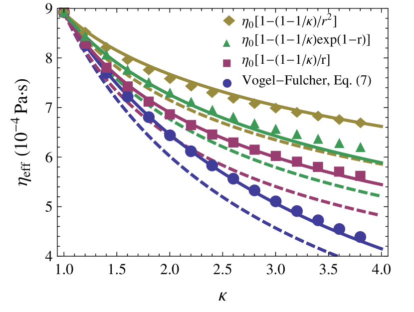
Figure 1: Comparison of analytical predictions of the scalar toy model to numerical results from the differential shell method (symbols) for exemplary long-ranged radial viscosity profiles $\eta(r)$ with $\kappa\equiv\eta(r\to\infty)/\eta(r=R)$ in a parameter regime of potential practical interest. While the simplest version of the model (dashed lines), which employs a constant calibration factor, exhibits noticeable systematic errors, the more elaborate version (solid line), corresponding to Eq. (12), should be sufficiently accurate for practical applications.

An analytically tractable expression for the effective friction coefficient $\zeta_{\rm HBM}$ as a function of temperature finally results from a combination of the calibrated model with Eq. (4) and a phenomenological expression for the temperature dependence of the solvent viscosity such as

$$\eta(T)=\eta_{\infty}\exp[A/(T-T_{\rm VF})]$$ (7)

(e.g. for water; but power-laws could be processed just as well). The effective friction can be reinterpreted in terms of an effective solvent viscosity $\eta_{\rm HBM}\equiv\zeta_{\rm HBM}/6\pi R$ that replaces $\eta_{0}$ in Eq. (2) under non-isothermal conditions. For reduced temperature increments $\theta\equiv\Delta T/(T_{0}-T_{\rm VF})<1$ the result is well approximated by its truncated Taylor series supplement

$$\begin{split}\frac{\eta_{0}}{\eta_{\rm HBM}}\approx 1&+\frac{193}{486}\left[\ln\frac{\eta_{0}}{\eta_{\infty}}\right]\theta\\ &-\left[\frac{56}{243}\ln\frac{\eta_{0}}{\eta_{\infty}}-\frac{12563}{118098}\ln^{2}\frac{\eta_{0}}{\eta_{\infty}}\right]\theta^{2}\;.\end{split}$$ (8)

This provides the wanted generalization of Eqs. (1-2).

To turn Eqs. (1-3) into a fully predictive Markov model of hot Brownian motion, the remaining task is to compute, in the same spirit, an appropriate effective temperature $T_{\rm HBM}$ to replace $T_{0}$ in Eq. (3). In other words, we aim at establishing a generalized non-equilibrium fluctuation-dissipation relation for Brownian motion in a co-moving radial temperature gradient. In analogy to the better understood situation in globally isothermal non-equilibrium steady states baiesi-maes-wynants:2009 , we expect to retrieve the fluctuation-dissipation relation only after excluding the “housekeeping heat” from the entropy balance; i.e. the heat constantly flowing from the particle to infinity to maintain the temperature gradient. All we have to consider is the minuscule excess dissipation associated with the damped motion of the Brownian particle. In this respect, it is crucial to appreciate the long-range correlated character of the hydrodynamic flow, which affects both dissipation and thermal fluctuations. It also helps in setting up a systematic coarse-grained calculation by extending the standard framework of fluctuating hydrodynamics hauge-martin_lof:73 to moderate temperature gradients rings-kroy:unpub .

In simple terms, the process of Brownian motion can be rephrased as a constant transformation of some thermal energy from the solvent into an equal amount of kinetic energy for the Brownian particle and vice versa. In a stationary situation the mutual energy transfer must be balanced to obey the first law. More precisely, the spatial integral over the local excess dissipation $\dot{q}(\mathbf{r})$ — i. e. the heat created (per unit of time) by the solvent flow at position $\mathbf{r}$ in response to the movement of the Brownian particle — must on average match the rate of kinetic energy transfer $\dot{W}_{\rm p}$ to the particle,

$$\langle\dot{W}_{\rm p}\rangle=\int\!\text{d}\mathbf{r}\;\langle\dot{q}(\mathbf{r})\rangle\;.$$ (9)

Moreover, to respect the second law, the motion must not cause a net average entropy change, which was the origin of major reservations against the modern interpretation of Brownian motion till the early 20th century. However, this only means that one has to make sure that the integral over the local entropy flux to the solvent — i. e. the local dissipation rate $\dot{q}(\mathbf{r})$ divided by the local solvent temperature $T(\mathbf{r})$ — equals on average the entropy flux $\dot{S}_{\rm p}=\dot{W}_{\rm p}/T_{\rm HBM}$ conferred to the Brownian particle:

$$\int\!\text{d}\mathbf{r}\;\frac{\langle\dot{q}(\mathbf{r})\rangle}{T(\mathbf{r})}=\frac{1}{T_{\rm HBM}}\int\!\text{d}\mathbf{r}\;\langle\dot{q}(\mathbf{r})\rangle\;.$$ (10)

This then defines the wanted effective Brownian temperature $T_{\rm HBM}$, if the dissipation $\dot{q}(\mathbf{r})$ is expressed in terms of the local viscosity $\eta(\mathbf{r})$ and $\nabla\mathbf{u}(\mathbf{r})$. Within our scalar model $\dot{q}(\mathbf{r})=\eta(r)[\partial_{r}u_{r}(r)]^{2}/2$, hence

$$T_{\rm HBM}=\left.\int\!\text{d}\mathbf{r}\;\eta(r)\langle(\partial_{r}u_{r})^{2}\rangle\!\right/\!\!\!\int\!\text{d}\mathbf{r}\;\frac{\eta(r)}{T(r)}\langle(\partial_{r}u_{r})^{2}\rangle\;.$$ (11)

For the special case of a temperature-independent constant viscosity $\eta_{0}$ this reduces to the simple explicit expression

$$T_{\rm HBM}=\Delta T/\ln(1+\Delta T/T_{0})\;.$$ (12)

The analytical expression generalizing this to the main case of interest, a viscosity $\eta(r)$ that varies radially according to Eqs. (4) & (7), is given in Ref. supplement . For small temperature increments $\Delta T\ll T_{0}$ a practical approximation is

$$T_{\rm HBM}\approx T_{0}+\Delta T/2-\left[1-\ln(\eta_{0}/\eta_{\infty})\right]\Delta T^{2}/(24T_{0})\;.$$ (13)

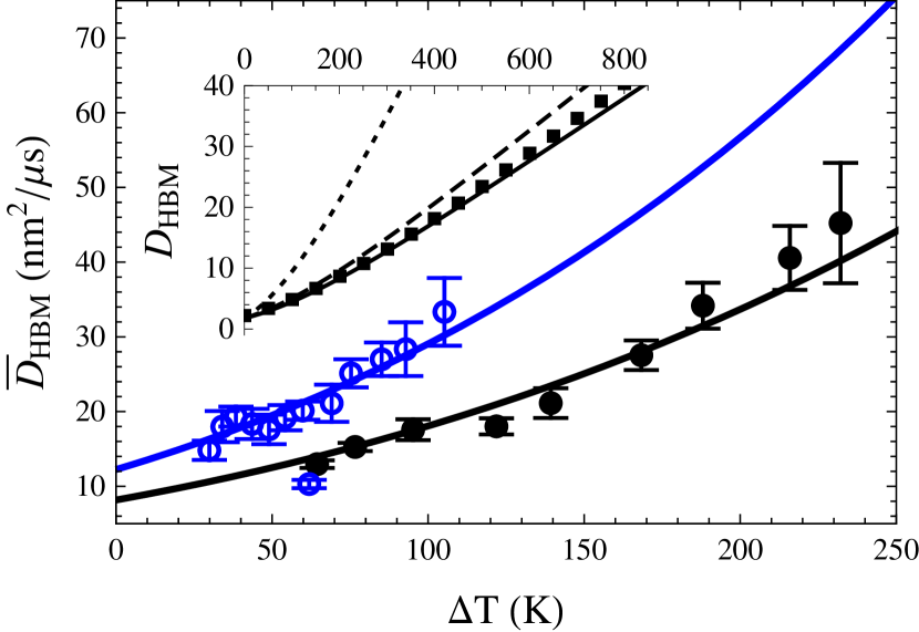
Figure 2: The effective diffusion coefficient $\bar{D}_{\rm HBM}(\Delta T)$ of hot gold nano-particles traversing a laser focus in water: experimental data (open/closed symbols for $R=40/60\;$nm) versus analytical predictions from the scalar model (solid lines); for solvent and focus parameters and the error bars see Ref. supplement . Inset: $D_{\rm HBM}(\Delta T)$ according to numerical predictions from the differential shell method (squares), analytical solutions of the scalar model (corresponding to the lowest pair of curves in Fig. 1), and the naive suggestion to identify the HBM parameters with the conditions at the particle surface (dotted); the agreement between the symbols and the solid line demonstrates the equivalence of Eqs. (10) & (11).

A hot Brownian particle described by Eqs. (2-3) with $\eta_{0}$ and $T_{0}$ replaced by the corresponding effective quantities $\eta_{\rm HBM}$ and $T_{\rm HBM}$ from Eqs. (12) & (15) performs a random diffusive motion characterized by an effective diffusion coefficient $D_{\rm HBM}$ obeying the generalized Stokes–Einstein relation

$$D_{\rm HBM}=\frac{k_{B}T_{\rm HBM}}{6\pi\eta_{\rm HBM}R}\;.$$ (14)

This prediction is tested against the numerical differential shell method in the inset of Fig. 2. The good agreement demonstrates the equivalence of Eqs. (10) and (11).

In order to test Eq. (14) also experimentally, we used a photothermal microscopy setup with gold nano-particles in water, as described in Refs. radunz-etal:2009 ; supplement . Particles passing through the common focal volume of a heating and a detection laser beam leave a trace of photothermal bursts in the detector, which encodes information about the diffusivity. The spatially inhomogeneous heating power in the laser focus implies, via Eq. (14), that the diffusion in the focus is inhomogeneous. (A wider focus of the heating laser would avoid this complication but is generally undesirable as one wants to minimize sample irradiation.) We therefore pursue a first-passage time approach to determine the apparent effective diffusion coefficient $\bar{D}_{\rm HBM}$ of inhomogeneous hot Brownian motion from the burst durations, which we identify with the transit times of the particles passing through the focus volume . The time periods $\tau$ during which the photothermal signal supersedes a fixed percentage of the maximum signal at a given laser power are recorded for a large number of photothermal bursts. The diffusion coefficient is then extracted from the exponential decay of the obtained transit time distribution $P(\tau)$ at large $\tau$ ko:1997 ; nagar-pradhan:2003 ; supplement ,

$$\ln P(\tau\to\infty)\propto-\bar{D}_{\rm HBM}\tau\;.$$ (15)

Figure 2 shows the result of such measurements for various laser powers. The surface temperatures $T_{\rm s}=T_{0}+\Delta T$ have been calculated from known quantities, namely the incident laser intensity, the optical absorption coefficient of the particles, and the heat conductivity of the solvent radunz-etal:2009 . Due to our limited knowledge of the focus geometry, the factor of proportionality in Eq. (15) could not be determined precisely, though. We therefore took the liberty to multiply each data set by an overall factor to optimize the fit supplement . Yet, the good agreement of the functional dependence with the prediction provides strong support for our analytical results, over a considerable temperature range. At the same time, it establishes hot Brownian motion as a robust and manageable tracer technique.

In summary, by introducing appropriate effective friction (viscosity) and temperature parameters $\zeta_{\rm HBM}$ ($\eta_{\rm HBM}$) and $T_{\rm HBM}$, for which we provided explicit analytical expressions in Eqs. (12) and (15), the convenient Markovian description of Brownian motion in terms of Eqs. (2-3) could be extended to non-equilibrium conditions, where the temperature of the Brownian particle differs from that of the solvent. While Eqs. (2-3) are recovered in the isothermal limit, the general predictions differ significantly from what might have been guessed from simple rules of thumb and provide an instructive illustration of the general dictum that hydrodynamic boundary conditions should not be confused with the microscopic conditions at the boundary . We sidestepped some technical difficulties of the corresponding problem in fluctuating hydrodynamics by introducing an analytical toy model that we calibrated with help of more elaborate analytical and numerical calculations. Our analytical prediction for the effective diffusion coefficient, based on the generalized Stokes–Einstein relation in Eq. (14), compares favorably with our measurements of gold nano-particles depicted in Fig. 2 and thus provides a convenient basis for photothermal tracer techniques bericiaud-etal:2004 ; radunz-etal:2009 with a high potential of complementing corresponding fluorescence-based methods applied in many fields from nano-technology to biology.

Supplementary Material

The supplementary material is organized as follows. In Section 1, we revisit Stokes’ problem of the viscous drag on a sphere for an inhomogeneous viscosity $\eta(r)$ approximated by (i) a step function and (ii) a staircase, from which we obtain numerically exact solutions for $\eta_{\rm HBM}$ in the continuum limit. In Section 2, we solve the scalar toy model. Comparison with (i) suggests an improved calibration. Section 3 provides the complete expression for the diffusion coefficient $D_{\rm HBM}$ and Section 4 the generalization $\bar{D}_{\rm HBM}$ for inhomogeneous hot Brownian motion. Section 5 summarizes some phenomenological parameter values. For complete derivations and a more comprehensive discussion see S (1).

I 1. Shell and differential shell method for Stokes’ problem

Stokes’ classical problem of finding the friction coefficient $\zeta$ of sphere of radius $R$ in a homogeneous Newtonian fluid of known viscosity $\eta_{0}$ has a well-known solution: $\zeta=6\pi\eta_{0}R$. As stated in the main text, we wish to generalize this result to radially varying viscosities $\eta(r)$. We consider (i) a step profile and (ii) a staircase profile. In both cases the solution for the velocity $\mathbf{u}$ and pressure $p$ take on the form

$$u_{r} =\left(a_{0}+\frac{a_{1}}{r}+a_{2}r^{2}+\frac{a_{3}}{r^{3}}\right)\cos\theta$$ (S1)

$$u_{\theta} =-\left(a_{0}+\frac{a_{1}}{2r}+2a_{2}r^{2}-\frac{a_{3}}{2r^{3}}\right)\sin\theta$$

$$p =p_{0}+\left(\frac{a_{1}}{r^{2}}+10a_{2}r\right)\eta\cos\theta$$

in each of the spatially homogeneous regions.

1. The step profile $\eta(r)=\eta_{\rm s}\left[1+(\kappa-1)\Theta(r-b)\right]$ jumping from $\eta_{\rm s}$ to $\eta_{0}\equiv\kappa\eta_{\rm s}$ at $r=b$. The coefficients $a_{0}\ldots a_{3}$ in the two domains $r<b$ and $r>b$ follow from the continuity conditions for the velocity and the stress at the jump discontinuity.

2. Similarly, the solution for the staircase profile is characterized by a set $(a_{0},a_{1},a_{2},a_{3})_{j}$ of coefficients and corresponding continuity conditions. Along the lines of similar work for inhomogeneous elastic media S (2), we take the limit of an infinite staircase of infinitesimally thin shells, and the coefficients become radial functions $a_{i}(r)$ that can generally only be evaluated numerically. This differential shell method yields the (inverse) effective friction coefficient

   $$\zeta^{-1}=\left.a_{0}(R)-a_{1}(R)R^{-1}+a_{2}(R)R^{2}+a_{3}(R)R^{-3}\right|_{F=1},$$ (S2)

   evaluated at a reduced force of $F=1$. (The friction coefficient is defined by the force, viz. the stress integrated over the particle surface, divided by the velocity relative to the fluid at infinity.) Results for some exemplary viscosity profiles are shown as symbols in Fig. 1 of the main text.

II 2. Scalar Toy Model

To find a generally applicable analytically tractable approximation for the friction coefficient $\zeta_{\rm HBM}$ we resort to a toy model that evades the technical difficulties related to the vector character of the fluid velocity but retains the long-ranged nature of the hydrodynamic flow field. We replace $\mathbf{u}(\mathbf{r})$ by a fictitious diffusing scalar $u(\mathbf{r})$ without direct physical significance, for which Eq. (5) reduces to $\nabla\cdot\eta(r)\nabla u(\mathbf{r})=0$. Hence, we seek a radially symmetric solution $u_{r}$ of Eq. (6), $[\partial_{r}+2/r+(\partial_{r}\ln\eta)]\partial_{r}u_{r}=0$. Integrating twice,

$$u_{r}(r)=K\int_{r}^{\infty}\frac{\text{d}r^{\prime}}{r^{\prime 2}\eta(r^{\prime})},\quad K=const.\;,$$ (S3)

which simplifies to $K/\eta_{0}r$ for homogeneous viscosity $\eta(r)\equiv\eta_{0}$, and can be expressed in the following closed form for $T(r)=T_{0}+R\Delta T/r,\,\Delta T>0$ and the Vogel-Fulcher temperature-dependence of the viscosity specified in Eq. (7) of the main text:

$$u_{r}(r)=-\frac{K\alpha}{\beta}\left[\frac{e^{-x}}{x}-\mathrm{Ei}(-x)\right]_{\frac{\alpha}{1+\beta/r}}^{\alpha}$$ (S4)

The abbreviations $\alpha\equiv B/T_{0}$ and $\beta\equiv R\Delta T/T_{0}$ have been used. The effective friction coefficient is

$$\zeta_{\text{HBM}}=\frac{4\pi R^{2}\eta\partial_{r}u_{r}(R)}{u_{r}(R)}=\frac{4\pi K}{u_{r}(R)}\;.$$ (S5)

For homogeneous viscosity $\eta(r)\equiv\eta_{0}$ it degenerates to $4\pi\eta_{0}R$, indicating a mismatch by a factor of $3/2$ compared to exact result. The simplest calibration of the scalar model consists in correcting this constant factor such as to match the predictions in the homogeneous case. In the inhomogeneous case, $\Delta T>0$, we express Eq. (S5) by the corresponding effective viscosity $\eta_{\rm HBM}$. Including the mentioned factor of $3/2$ and making the temperature dependence (see Section 5) explicit, we have (with the abbreviation $T^{\ast}\equiv T-T_{\text{VF}}$)

$$\frac{\eta_{0}}{\eta_{\text{HBM}}}=\frac{e^{A/T^{\ast}}\left[A\left(\text{Ei}\left(-\frac{A}{T^{\ast}+\Delta T}\right)-\text{Ei}\left(-\frac{A}{T^{\ast}}\right)\right)+(T^{\ast}+\Delta T)e^{-\frac{A}{T^{\ast}+\Delta T}}\right]-T^{\ast}}{\Delta T}\;.$$ (S6)

This result features as the lowest dashed line in Fig. 1 of the main text; analogous calculations for different viscosity profiles $\eta(r)$ provide the other dashed lines in the figure. Viscosity profiles of the form $\eta(r)=\eta_{0}[1-(1-1/\kappa)(R/r)^{n}],\,n\in\mathds{N}$ result in

$$\frac{\eta_{0}}{\eta_{\text{HBM}}}=\,_{2}F_{1}\left(1,\frac{1}{n};1+\frac{1}{n};\frac{\kappa-1}{\kappa}\right)\;,$$ (S7)

where ${}_{2}F_{1}(a,b;c;z)$ denotes the hypergeometric function. For the two cases $n=1,2$, shown in Fig. 1 of the main text, $\eta_{0}/\eta_{\mathrm{HBM}}$ can be expressed as

$$\frac{\eta_{0}}{\eta_{\text{HBM}}}=\frac{\kappa\ln\kappa}{\kappa-1}\;,\qquad(n=1)$$ (S8)

and

$$\frac{\eta_{0}}{\eta_{\text{HBM}}}=\frac{\kappa\,\mathrm{arctanh}\sqrt{\frac{\kappa-1}{\kappa}}}{\sqrt{\kappa(\kappa-1)}}\;,\qquad(n=2)\;.$$ (S9)

For a more sophisticated calibration of the scalar model, we consider again the step profile (i). The scalar model with the simple calibration predicts the friction coefficient

$$\zeta=\frac{b/R}{1+(b/R-1)\kappa}6\pi\eta_{0}R$$ (S10)

By $\kappa\equiv\eta_{0}/\eta_{\rm s}$, we denote the ratio of the ambient viscosity and the solvent viscosity at the surface of the Brownian particle, as before. Note that the trivial limits $\kappa\to 1$ and $b\to R$, and the limit $\kappa\to 0$ of a frozen surface layer, are correctly obtained, whereas the joint limit $\kappa\to\infty$ and $b\to R$, corresponding to a particle coated with an infinitesimal superfluid layer, is ambiguous. To recover the correct slip boundary condition ($\zeta=4\pi\eta R$) in this case, one has to take this limit along the curve defined by $b/R=1+1/2\kappa$. If we impose this constraint on Eq. (S10), the calibration factor to match it with the exact solution, which we obtain as described in the previous section, viz. Eq. (S2), is found as

$$\frac{3\left(80\kappa^{4}+80\kappa^{3}+60\kappa^{2}+20\kappa+3\right)}{200\kappa^{4}+250\kappa^{3}+205\kappa^{2}+65\kappa+9}$$ (S11)

With this more elaborate calibration, the analytical predictions of the scalar model (solid lines in Figures 1 and 2 of the main text) practically coincide quite universally over a broad range of $\kappa$ with the numerical predictions obtained from the differential shell method.

For moderate temperature increments $\Delta T\approx 0\dots 150\,$K, which are probably of greatest interest in practical applications, the result can be further simplified by expanding Eqs. (S6,S11) in a series in $\theta\equiv\Delta T/(T_{0}-T_{\mathrm{VF}})$,

$$\frac{\eta_{0}}{\eta_{\rm HBM}}=1+\frac{193}{486}\left[\ln\frac{\eta_{0}}{\eta_{\infty}}\right]\theta-\left[\frac{56}{243}\ln\frac{\eta_{0}}{\eta_{\infty}}-\frac{12563}{118098}\ln^{2}\frac{\eta_{0}}{\eta_{\infty}}\right]\theta^{2}+O(\theta^{3}).$$ (S12)

Truncation after the second order yields Eq. (8) of the main text. In Fig. S1, it is compared to the full expression and to the result obtained with the simple calibration by the constant factor $3/2$.

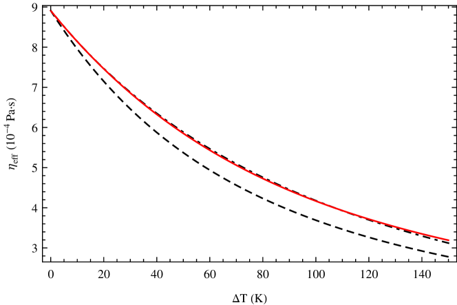
Figure S1: Temperature dependence of the effective viscosity according to the scalar model, Eq. (S5): simplest calibration by a constant factor to match the isothermal limit (dashed); improved calibration with Eqs. (S6-S11) (dash-dotted); the truncated Taylor series of Eq.(S12) (solid).

III 3. Effective diffusion coefficient

Inserting the solution $u(r)$ of the scalar model from Eq. (S4) into Eq. (11) of the main text yields the effective temperature

$$T_{\mathrm{HBM}}=\frac{Ae^{-\frac{X\left(T_{0}(\Delta T+T_{0})-T_{\mathrm{VF}}^{2}\right)}{T_{0}T_{\mathrm{VF}}}}\left[(T_{0}-T_{\mathrm{VF}})e^{\frac{X(\Delta T+2T_{0}-2T_{\mathrm{VF}})}{T_{0}}}\left(\text{Ei}\bigl{(}-\frac{A}{T_{0}}\bigr{)}-\text{Ei}\bigl{(}\frac{AX}{T_{0}Y}\bigr{)}\right)\bigr{/}T_{0}-e^{A/T_{0}}/X-e^{X-\frac{T_{\mathrm{VF}}X}{T_{0}}}/Y\right]}{e^{AZ}\left(\text{Ei}\bigl{(}\frac{AX}{T_{0}Y}\bigr{)}-\text{Ei}\bigl{(}-\frac{A}{T_{0}}\bigr{)}\right)+\text{Ei}\bigl{(}-\frac{A}{T_{\mathrm{VF}}}\bigr{)}-\text{Ei}\bigl{(}(\Delta T+T_{0})XZ\bigr{)}},$$ (S13)

with the following abbreviations

$$X\equiv\frac{A}{\Delta T+T_{0}-T_{\text{VF}}},\quad Y\equiv\frac{A}{T_{\text{VF}}-T_{0}},\quad Z\equiv\frac{1}{T_{0}}-\frac{1}{T_{\text{VF}}}\;.$$ (S14)

Again, a simpler approximate expression is expected to suffice for most practical purposes, in particular with regard to the various minor contributions that were neglected altogether in our approach. For moderate temperature increments $\Delta T\ll T_{0}$ a Taylor expansion yields

$$\frac{T_{\rm HBM}}{T_{0}}=1+\frac{\Delta T}{2T_{0}}+\left[\ln\Bigl{(}\frac{\eta_{0}}{\eta_{\infty}}\Bigr{)}-1\right]\frac{\Delta T^{2}}{12T_{0}^{2}}+O\Bigl{(}\frac{\Delta T^{3}}{T_{0}^{3}}\Bigr{)}\;.$$ (S15)

The semi-phenomenological approximation quoted in Eq. (13) of the main text is obtained by dividing the second-order contribution by 2. As illustrated by the comparison with the full expression, Eq. (S13), in Fig. S2, the deviations of the approximate expression Eq. (13) from Eq. (S13) are insignificant at the present overall level of accuracy if $\Delta T$ is in the range $0\ldots 150$ K.

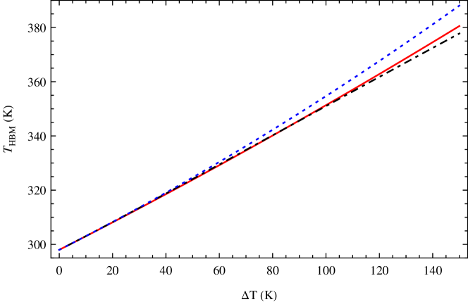
Figure S2: Dependence of various expressions for the effective Brownian temperature $T_{\mathrm{HBM}}$ on the temperature increment $\Delta T\equiv T_{\rm s}-T_{0}$: the calibrated scalar model given in Eq. (S13) (dot-dashed); the second order Taylor expansion Eq. (S15) (dotted, blue); and the semi-phenomenological approximation given in Eq. (13), and displayed in Fig. 2, of the main text (solid, red). In contrast to the truncated Taylor series Eq. (S15), the semi-phenomenological expression has no significant errors over the practically relevant temperature range.

Inserting $T_{\mathrm{HBM}}$ from Eq. (S13) and the effective viscosity $\eta_{\mathrm{HBM}}$ from Eq. (S6) into the generalized Stokes–Einstein relation $D_{\mathrm{HBM}}=k_{\mathrm{B}}T_{\mathrm{HBM}}/(6\pi\eta_{\mathrm{HBM}}R)$, Eq. (14) of the main text, we obtain the effective diffusion coefficient

$$\begin{split}D_{\mathrm{HBM}}&=\frac{\exp\left[-X(\Delta T+T_{0}+T_{\text{VF}})/T_{\text{VF}}\right]}{6\pi\eta_{\infty}RT_{0}\Delta T\left(\text{Ei}\bigl{(}\frac{A(\Delta T+T_{0})X}{T_{0}T_{\text{VF}}Y}\bigr{)}+e^{AZ}\left[\text{Ei}\bigl{(}-\frac{A}{T_{0}}\bigr{)}-\text{Ei}\bigl{(}\frac{AX}{T_{0}Y}\bigr{)}\right]-\text{ Ei}\bigl{(}-\frac{A}{T_{\text{VF}}}\bigr{)}\right)}\times\\ &\negthickspace\negthickspace\negthickspace\left\{\left.A(T_{0}-T_{\text{VF}})e^{\frac{X(\Delta T+2T_{0}-T_{\text{VF}})}{T_{0}}}\left[\text{Ei}\Bigl{(}\frac{AX}{T_{0}Y}\Bigr{)}-\text{Ei}\Bigl{(}-\frac{A}{T_{0}}\Bigr{)}\right]+T_{0}\left[\Delta Te^{\frac{A+T_{\text{VF}}X}{T_{0}}}-(T_{0}-T_{\text{VF}})\left(e^{X}-e^{\frac{A+T_{\text{VF}}X}{T_{0}}}\right)\right]\right\}\times\right.\\ &\negthickspace\negthickspace\negthickspace\left\{-Ae^{X}\text{Ei}(Y)+Ae^{X}\text{Ei}(-X)+\Delta T-T_{0}e^{X+Y}+T_{0}+T_{\text{VF}}e^{X+Y}-T_{\text{VF}}\right\}\;,\end{split}$$ (S16)

with abbreviations as above. As illustrated in Fig. S3, a satisfying approximation is indeed again obtained by use of the simple approximate expressions for $T_{\mathrm{HBM}}$ and $\eta_{\mathrm{HBM}}$ from Eqs. (8) & (13) of the main text, respectively. This is how the curves in Fig. 2 of the main text were generated.

Figure S3: Temperature dependence of the effective diffusion coefficient $D_{\mathrm{HBM}}(\Delta T)$ from the scalar model, as given in Eq. (S16) (dot-dashed), and in the approximation obtained by inserting the individual approximations of $T_{\mathrm{HBM}}$ and $\eta_{\mathrm{HBM}}$ from Eqs. (8) & (13) of the main text into the generalized Stokes-Einstein formula (solid, red).

IV 4. Apparent diffusion coefficient for inhomogeneous heating power

In practical applications diffraction usually limits the experimental realization of a spatially uniform heating rate within the observation volume. Therefore, the apparent diffusion coefficient deduced from the transit time statistics of the particles passing through the focus involves some implicit averaging over a spatially heterogeneous $D_{\mathrm{HBM}}(\mathbf{r})$. In the following, we derive a theoretical expression for this average.

First, the local diffusion coefficient $D_{\mathrm{HBM}}(\mathbf{r})$ follows immediately from the heating power density $I(\mathbf{r})$ via Eq. (S16) by noting that $\Delta T(\mathbf{r})\propto I(\mathbf{r})$ if the absorption coefficient of the particle is temperature insensitive. Assuming a radially symmetric heating power distribution in the focus, the appropriate averaging procedure is similar to that for a particle released at the center of the focus, which can be traced back to a standard first-passage-time problem S (3, 4). The distribution $P(\mathbf{r},t)$ of escape times for the particle is obtained by solving the Smoluchowski equation with an absorbing boundary condition at the boundary ${\cal B}$ of the focus volume,

$$\frac{\partial P}{\partial t}=\nabla\cdotp D(r)\nabla P,\quad P(\mathbf{r},0)=\delta(\mathbf{r}-\mathbf{r}_{0}),\quad P(\mathbf{r},t)=0\text{ on }{\cal B}$$ (S17)

The spherically symmetric boundary value problem for the escape time $\tau_{\rm p}(\mathbf{r})=\tau_{\rm p}(r)$ of a particle starting at position $\mathbf{r}$ is

$$\tau_{\rm p}^{\prime}(2/r+\partial_{r})D+D\tau_{\rm p}^{\prime\prime}=-1\quad\text{with}\quad\tau_{\rm p}(\mathbf{r})=0\text{ on }{\cal B}\;,$$ (S18)

which has the general solution

$$\tau_{\rm p}(r)=\int_{\omega}^{r}\left(\frac{c}{D(r^{\prime})r^{\prime 2}}-\frac{r^{\prime}}{3D(r^{\prime})}\right)\mathrm{d}r^{\prime}\;,$$ (S19)

$\omega$ being the radius of the focus volume and $c$ a constant of integration. For the escape problem of a particle starting in the center of the focus, $c=0$ is required by $\tau_{\rm p}(0)<\infty$. The apparent diffusion coefficient thus reads

$$\bar{D}_{\mathrm{HBM}}=\omega^{2}/6\tau_{\rm p}(0)\;.$$ (S20)

For the related transit problem, which is of interest for our transit time analysis, the situation is slightly more complicated. The most likely transit paths are only touching or barely entering the focus, so that the transit time distribution $P_{\rm transit}(t)$ diverges at $t=0$. However, the characteristic transit time $\tau_{\rm t}$ may be extracted from the experimentally obtained transit time distribution by fitting the asymptotic law $P_{\rm transit}(t\gg 0)\sim t^{-3/2}\exp[-t/\tau_{\rm t}]$ S (5, 6). The stochastic errors inferred from the fits are displayed as error bars in Fig. 2 of the main text. The apparent diffusion coefficient follows from $\tau_{\rm t}$ as

$$\bar{D}_{\mathrm{HBM}}=\omega^{2}/\pi^{2}\tau_{\rm t}\;,$$ (S21)

for spherical focus geometry. In practice, the focus is usually more elongated along the optical axis than transverse to it, so that it may be better approximated by a cylinder, in which case

$$\bar{D}_{\mathrm{HBM}}=\omega^{2}/\alpha_{1}^{2}\tau_{\rm t}\;,$$ (S22)

where $\alpha_{1}$ denotes the first zero of the Bessel function of the first kind of order zero. The different numerical factors in the last two expressions therefore provide a lower bound for the systematic numerical uncertainties involved in the determination of the absolute value of $\bar{D}_{\mathrm{HBM}}$.

A typical experiment yields a time series of photothermal bursts S (7). Their intensity is proportional to the local power densities of the lasers used for heating the particle and detecting the induced refractive index change, respectively. Here, an uncertainty arises since the focus geometry cannot be controlled or determined precisely in the diffusion experiment. A nominal lateral focus size $\rho=300\,$nm has therefore been estimated by fitting a Gaussian intensity profile $\propto\exp[-r^{2}/(2\rho^{2})]$ to the photothermal image of single immobilized gold nano-particles obtained with the same setup. As the axial extension of the focus is usually large compared to the lateral one (about $1\,\mu$m), the focal volume is approximated by a cylindrical shape, corresponding to Eq. (22). Particles are identified as “in the focus” if the signal intensity surpasses a certain threshold set to a fixed percentage of the maximum signal of the whole time trace of bursts. The threshold therefore defines the actual focus size $\omega$ relevant for the burst width analysis, which stays constant during the measurements of a given sample, due to scaling of the threshold with the maximum signal. In Fig. 2 of the main text, we use the value of $\omega$ as a freely adjustable overall fit parameter to match the experimental data with the theoretical prediction for $\bar{D}_{\mathrm{HBM}}$ and find $\omega\approx 250\,$nm for the $R=60\,$nm particles and $\omega\approx 170\,$nm for the $R=40\,$nm gold nano-particles. Note that $\omega$ may generally differ between the measurements of different samples (viz. particle sizes) due to variations in the signal-to-noise ratio and the sample geometry.

V 5. Parameters for the solvent viscosity

Parameter values used for all graphs throughout the main text and the supplementary material:

ambient temperature $$T_{0} =298\,\mathrm{K}$$

dynamic viscosity of water $$\eta(T) =\eta_{\infty}\exp[A/(T-T_{\mathrm{VF}})]$$

with $$\eta_{\infty} =0.0298376\,\mathrm{mPa\cdotp s}$$

$$A =496.889\,\mathrm{K}$$

$$T_{\mathrm{VF}} =152.0\,\mathrm{K}$$

References

- S (1) D. Rings et al., unpublished.
- S (2) A. J. Levine and T. C. Lubensky, Phys. Rev. E 65, 011501 (2001).
- S (3) S. Revathi and V. Balakrishnan, J. Phys. A 26, 5661 (1993).
- S (4) R. Zwanzig, Nonequilibrium Statistical Mechanics (Oxford University Press, USA, 2001).
- S (5) D. S. Ko et al., Chem. Phys. Lett. 269, 54 (1997).
- S (6) A. Nagar and P. Pradhan, Physica A 320, 141 (2003).
- S (7) R. Radünz, D. Rings, K. Kroy, and F. Cichos, J. Phys. Chem. A 113, 1674 (2009).