Cold atom dynamics in crossed laser beam waveguides

Abstract

We study the dynamics of neutral cold atoms in an $L$-shaped crossed-beam optical waveguide formed by two perpendicular red-detuned lasers of different intensities and a blue-detuned laser at the corner. Complemented with a vibrational cooling process this setting works as a one-way device or “atom diode”.

I Introduction

Controlling the microscopic motion of atoms in gas phase is one of the main goals of atomic physics and atom optics for fundamental studies and for applications such as metrology, precise spectroscopy, the atom laser, or quantum information. Different control objectives have been achieved with optical and/or magnetic fields during the last two decades. The phase-space domain of the atom can be restricted by different traps, and the location manipulated by optical tweezers. The modulus of the velocity and its spread have been controlled as well by several stopping or cooling techniques, and its direction by magnetic waveguides combined into atom chips and integrated circuits review , or by optical waveguides Birkl ; laser1 ; laser2 ; laser3 . The implementation of complex geometries for atom transport is a challenging objective that may open the way to new interferometers and integrated quantum information processing review . In particular waveguide bends are basic elements that have been investigated experimentally and theoretically bendsH ; bendsB ; bendsL ; bendsB03 ; bendsB04 .

Aside from modulus and direction, the control of the remaining element of the atom velocity as a vector, its sense or orientation (say to the right or left for a given direction), has been undertaken much more recently with theoretical proposals and experimental prototypes of atomic one-way barriers or “atom diodes” RM04 ; raizen05 ; dudarev05 ; RM06 ; RMR06q ; RMR06d ; RM07 ; Mark07 ; Mark08 ; ring ; Dan ; Science09 ; Dan2 . They are analogous to a semipermeable membrane or a valve, which let the atoms cross it one way (forward) and block their passage in the other one (backward). A conceptual precedent is the automated demon conceived long ago by Maxwell to achieve a differential of pressure between two parts of a vessel and demonstrate the statistical character of entropy RMR06d . Maxwell only specified the demon’s action, not its inner workings, whereas, more than one century later we are beginning to design and realize such devices. Applications that have motivated so far this research are the possibility to cool species without cyclic transitions raizen05 ; Science09 , or the construction of trapdoors and flow control in atomic chips and circuits RM04 . The existing methods are essentially one-dimensional (the controlled sense corresponds to a longitudinal or a radial velocity). A basic scheme consists on setting a barrier in one atomic level, e.g. the ground one. On one side of the barrier, say the left, the atom is excited adiabatically so as to avoid the ground state barrier. Adiabaticity is useful to make the transfer efficient and velocity independent in a broad range and to avoid the passage from the upper to lower level for atoms that approach the diode from the left RM06 . On the other side of the barrier the excited state is forced to decay so that an atom coming from the right is reflected by the barrier. One possible variant is to substitute the adiabatic step by optical pumping. It is also velocity independent in a broad range and precludes forced deexcitation on the wrong side. An irreversible step, which ideally may be reduced to the emission of one-photon, is essential to break time-reversal invariance, a necessary condition to realize a true one-way barrier. Any atom diode has of course certain limitations with respect to velocity working range, efficiency, width of the structure, or species and states that can be treated. For example, in a two-laser, optical prototype for Rubidium Dan ; Dan2 , the barrier produced some undesired heating because the internal hyperfine structure used does not allow for a sufficiently large detuning; the use of magnetic sublevels may avoid this effect but at the price of loosing many atoms because of the branching ratios during optical pumping raizen05 . While these limitations may or not be relevant depending on the intended application, it is desirable to investigate other mechanisms, surely subjected to different constraints.

In this paper we investigate two aspects of cold atom guiding and their possible combination into a single device: bends in $L$-shaped asymmetric guides and one-way motion. Most previous studies of bent waveguides have focused on magnetic implementations and symmetrical arms bendsH ; bendsB ; bendsB03 ; bendsB04 ; $X$-shaped optical waveguides have been investigated as beam splitters for interferometry Birkl ; Sam ; Gir . An experimental realization of an $X$-shaped asymmetrical beam splitter, with different potential depths in the two guides, has been also carried out Houde . We shall study here an optical, asymmetric realization of an $L$-shaped bend and determine the transfer between longitudinal, gap, and transverse energies. In addition, when combined with vibrational cooling the $L$-shaped guide provides a 2D one-way mechanism for one-way motion.

II Simple optical waveguide model

The proposed device consists of three horizontal Gaussian laser beams (see Fig. 1).

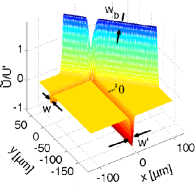
Figure 1: (Color online) Scheme of the potential created by a blue detuned and two red detuned lasers. $U^{\prime}=0.474$ $\mu$K.

Two of them are detuned to the red with respect to a transition between the atomic levels $g,\,e$ and play the role of waveguides for the ground state atoms along the $x$ and $y$ axes. We shall perform 2D simulations corresponding to a tight confinement in $z$ (vertical) direction, ignored hereafter, by an optical lattice. We have simplified the corresponding potentials neglecting the dependence with the longitudinal coordinate,

$$\tilde{U}(x,y) = -Ue^{-2y^{2}/w^{2}}\quad U>0,{\rm upper\;valley},$$ (1)

$$\tilde{U}^{\prime}(x,y) = -U^{\prime}e^{-2x^{2}/w^{\prime 2}}\quad U^{\prime}>U,{\rm lower\;valley}.$$ (2)

($w$ and $w^{\prime}$ are the waists.) This is reasonable within the Rayleigh length. It is as well a simplified treatment for combined magneto-optic waveguides laser1 in which the longitudinal potential dependence is essentially suppressed by cancellation between a repulsive magnetic potential and an attractive optical potential. Note that the assumed asymmetry in intensities creates “upper” and “lower” valleys in the potential energy surface.

A third laser, detuned to the blue, forms a barrier to redirect the atoms from the upper to the lower valleys blocking the passage to the red detuned arms along the positive-$x$ and positive-$y$ semiaxes. This laser is displaced slightly away from the coordinate origin and it is rotated an angle $\theta$ clockwise with respect to the $y$-axis, more on this below. The corresponding potential is

$$\tilde{U}_{b}(x,y)=U_{b}e^{-2[(x-x_{0})\cos{\theta}+(y-y_{0})\sin{\theta}]^{2}/w_{b}^{2}}.$$ (3)

We shall study the atom dynamics with quantum approaches (wavepackets and stationary methods), and with classical trajectories too since they provide a rather accurate description -in particular when an average over the transverse phase is performed- in a much shorter computation time than the quantum simulations. For a given incident longitudinal energy and vibrational state we do not perform “Ehrenfest” (one trajectory) classical simulations bendsB04 , but ensemble averages over all possible phases of transverse motion to avoid the sensitivity of classical trajectories with respect to the phase and better mimic the quantum results. The details are given in Appendix A.

We assume that there is no significant interference among the three beams so their potentials simply add up. This may be achieved e.g. by orthogonal polarizations of the red detuned lasers and/or different detunings that cause a fast time-dependent interference that averages out in the scale of the atomic motion Weiss .

In wavepacket computations, see Appendix B for numerical details, we assume that the wave function of the initial state factorizes into longitudinal and transversal functions,

$$\Psi(x,y,0)=\psi(x,0)\otimes\Phi(y,0).$$ (4)

For atoms incident in the upper channel the initial transverse wave function $\Phi(y,0)$ will be the ground state of the Gaussian potential, Eq. (1), which is calculated numerically by diagonalization of the Hamiltonian. In the longitudinal direction we choose a minimal uncertainty-product Gaussian,

$$\psi(x,0)=\frac{1}{(2\pi\sigma_{x}^{2})^{1/4}}e^{-(x-x_{i})^{2}/4\sigma_{x}^{2}}e^{ip_{i}x/\hbar},$$ (5)

where $\sigma_{x}$ is the width of the wavepacket and $x_{i}$ and $p_{i}$ the initial position and average longitudinal momentum respectively. For atoms incident from the lower channel a corresponding approach is used interchanging $x$ and $y$.

III Forward motion: passage from the upper to the lower valley

We shall discuss first the main factors that determine the passage of atoms from the upper valley, incident in the ground vibrational state, to the lower valley. All calculations are done for the mass of ${}^{87}Rb$ atoms.

The barrier position. If the barrier is too far from the crossing point of the waveguides, a well is formed due to the addition of the upper and lower valley potentials, Eq. (1) and Eq. (2), see Fig. 2b. This well allows for long lived chaotic (classical) trajectories and favours energy transfer among the degrees of freedom as well as reflection back into the upper valley. Displacing the blue detuned laser nearer to the origin the well is filled and the chaotic behavior and reflection are avoided. The wall should not be too close to the crossing though, as it would obstruct the upper valley and thus the atom passage, as in Fig. 2a. Between the two extremes there is a range of distances for which the well is suppressed without obstructing the upper valley, see Fig. 2c. Representative classical trajectories for the three cases are depicted in Fig. 2.

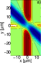
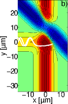
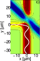
Figure 2: (Color online) Potential contour maps and representative trajectories for different wall positions. (a) $x_{0}=y_{0}=0$; (b) $x_{0}=y_{0}=5\mu$m; (c) $x_{0}=y_{0}=3\mu$m. Laser parameters: $U=0.158$ $\mu$K; $U^{\prime}=0.474$ $\mu$K; $U_{b}=0.948$ $\mu$K; $w=w^{\prime}=w_{b}=5.7$ $\mu$m and $\theta=45^{\circ}$. The 3D plot of Fig. 1 corresponds to case (c).

Barrier angle. Remarkably, the probability to pass from the upper to the lower valley shows a stable full-transmission plateau for a broad range of angles $\theta$. This is shown in Fig. 3 for wavepacket and classical trajectory calculations. The optimal choice of angle depends on its effect on energy transfer among longitudinal and transverse degrees of freedom, as discussed next.

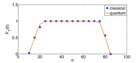
Figure 3: (Color online) Classical and quantum probability to find the atoms in the lower valley for different rotation angles of the blue detuned laser. Wavepacket parameters: $\sigma_{x}=2$ $\mu$m; $x_{i}=-15.88$ $\mu$m; $v_{i}=p_{i}/m=0.41$ cm/s. (For the classical calculation we average the fixed-energy probabilities with the momentum distribution of the longitudinal Gaussian.) Laser parameters: $U=0.158$ $\mu$K; $U^{\prime}=0.474$ $\mu$K; $U_{b}=0.948$ $\mu$K; $w=w^{\prime}=w_{b}=5.7$ $\mu$m and $x_{0}=y_{0}=3$ $\mu$m.

Vibrational excitation. If the atom passes to the lower valley, the asymmetric potential configuration favors its vibrational excitation (or “transverse heating”). For a transition from the ground state of the upper valley ($n=0$) to the $n^{\prime}$ vibrational state of the lower valley ($0\to n^{\prime}$ for short) conservation of energy, measured from the bottom of the lower valley, takes the form

$$E=K+V_{0}+\Delta=K^{\prime}+V_{n^{\prime}},$$ (6)

where $\Delta={U}^{\prime}-{U}$ is the gap between valleys, $K$, $K^{\prime}$ are the upper and lower kinetic energies, and $V_{0}$, $V_{n^{\prime}}$ the corresponding vibrational energies (measured from the bottom of each valley). Fig. 4 shows the (lower valley) average vibrational energy $\langle V^{\prime}\rangle$ versus the incident $K$ for several cases. Even for $K\approx 0$ the process is highly non-adiabatic (a simple 1D adiabatic treatment as in bendsL is therefore not valid here), and a significant fraction of the potential energy gap is converted into vibrational energy. As $K$ increases, the trajectories penetrate more on the reflecting blue wall so that the outgoing trajectories are further away from the bottom of the lower valley and vibrational excitation increases.

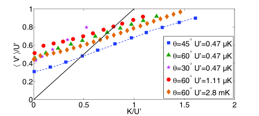
Figure 4: (Color online) Average final vibrational energy versus initial kinetic energy for different crossed-beam setups computed with classical trajectories. The dashed line is a quantum calculation (for monochromatic incident energy) showing good agreement with the classical one. Solid line: $K=\langle V^{\prime}\rangle$. Laser parameters: $w=w^{\prime}=1.03$ $\mu$m, $w_{b}=0.77$ $\mu$m, $x_{0}=y_{0}=0.41$ $\mu$m, $U=0.4$ mK and $U_{b}=5.2$ mK (rombs). Rest of cases: $w=w^{\prime}=w_{b}=5.7$ $\mu$m; $x_{0}=y_{0}=3$ $\mu$m; $U=0.158$ $\mu$K, $U_{b}=0.948$ $\mu$K (squares, triangles and stars), and $U_{b}=1.9$ $\mu$K (circles). The lines end when the transmission probability is no longer one. This full-transmission range increases with the angle and the depth of the lower valley.

The average $\langle V^{\prime}\rangle$ is essentially linear in $K$, at variance with a quadratic dependence found for circular bends bendsB . At the bottom of the lower valley the kinetic energy of a classical trajectory equals the total energy $K+\Delta+V_{0}$ (measured from the bottom of the lower valley). It may be split into $x$ and $y$ components taking into account the angle $\alpha$ of the velocity with the $y$ axis. The $x$-component is the final vibrational energy and it takes the form

$$V^{\prime}=E\sin^{2}(\alpha)=(\Delta+V_{0})\sin^{2}(\alpha)+K\sin^{2}(\alpha),$$ (7)

but $\alpha$ is roughly constant for a given set of potential parameters because of the relative flatness of the impact region at the waveguide corner. This region results from the combination of the dominant lower valley and barrier potentials.

Most lines in Fig. 4 are for classical-trajectory computations but we have also checked the good agreement with a fully quantum calculation in one case. To do so we have extracted the quantum, stationary (fixed energy) state-to-state transition probabilities $0\to n^{\prime}$, $(q_{n^{\prime}}/p)|T_{0n^{\prime}}(p)|^{2}$, from wavepacket calculations as explained in the Appendix B. Here $q_{n^{\prime}}$ is the longitudinal momentum in the lower valley for the vibrational state $n^{\prime}$ and $T_{0n^{\prime}}(p)$ the transmission amplitude for incident longitudinal momentum $p=\sqrt{2mK}$. In Fig. 5 we show the dependence of the quantum transmission probabilities versus the initial velocity. Note again, now in more detail, the increase of vibrational excitation with $p$. For sufficiently large energy this leads to escape from the trap.

Fig. 6a shows the total transmission probability $P_{T}=\sum_{n^{\prime}=0}^{N^{\prime}}\frac{q_{n^{\prime}}}{p}|T_{0n^{\prime}}(p)|^{2}$ versus initial velocity for $\theta=45^{\circ}$, $N^{\prime}$ being the maximal vibrational number in the lower valley. Note the good agreement between the quantum and classical calculations. $P_{T}$ is very stable, and only decays from one due to escape from the waveguide caused by the increasing transverse heating. In principle the energy threshold for escape is, from conservation of energy, $K+V_{0}+\Delta>U^{\prime}$ (solid vertical line on Fig. 6a), but the effective threshold occurs at higher energies, when $\langle V^{\prime}\rangle\approx U^{\prime}$, since the available initial total energy is transferred only partly into vibrational energy $\langle V^{\prime}\rangle$; a sign of the escape is the coincidence of decay of $P_{T}$ with the population of the highest vibrational level ($N^{\prime}=40$ for the chosen parameters). The velocity range for full forward transmission may be increased at will, according to Eq. (7), by increasing the gap $\Delta$, an example is shown below.

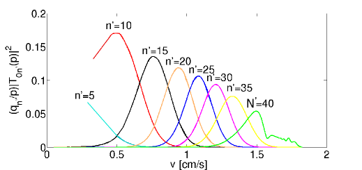
Figure 5: (Color online) The quantum transmission probabilities obtained from Eq. (18) for different vibrational levels of the lower guide versus the initial velocity. Laser parameters: $U=0.158$ $\mu$K; $U^{\prime}=0.474$ $\mu$K; $U_{b}=0.948$ $\mu$K; $w=w^{\prime}=w_{b}=5.7$ $\mu$m; $x_{0}=y_{0}=3$ $\mu$m and $\theta=45^{\circ}$.

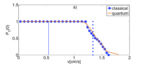
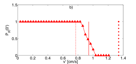
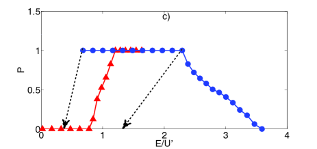
Figure 6: (Color online) (a) Classical and quantum probabilities to find the atoms in the lower valley when they start in the $n=0$ vibrational level of the upper valley, versus the initial longitudinal velocity. The vertical lines are the energy thresholds to escape from the guides (solid) and overcome the barrier (dotted). (b) Classical probability to find the atoms reflected in the lower valley when they start in the $n^{\prime}=0$ vibrational state of the lower valley versus the initial velocity ($v_{n^{\prime}}=q_{n^{\prime}}/m$). Vertical lines mark the energy thresholds to pass to the upper valley (dashed), escape from the guides (solid), and overcome the barrier (dotted). (c) Combination of (a) and (b). Blue circles: Transmission probability $P=P_{T}$ versus the total energy (measured from the bottom of the lower valley), the atoms start in the upper valley. Red triangles: $P=1-P_{R}$ versus the total energy of the sample, the atoms start in the $n^{\prime}=0$ vibrational level of the lower valley. Dashed arrow: It indicates the total energy that remains for backward motion after the (perfect) vibrational cooling process. Laser parameters: $U=0.158$ $\mu$K; $U^{\prime}=0.474$ $\mu$K; $U_{b}=0.948$ $\mu$K; $w=w^{\prime}=w_{b}=5.7$ $\mu$m; $x_{0}=y_{0}=3$ $\mu$m and $\theta=45^{\circ}$.

A second effect that may spoil the forward passage is the possibility to overcome the barrier when $K+V_{0}>U_{b}$ (we neglect here the lower valley potential). This threshold is higher than the former, and is marked by a vertical dotted line in Figs. 6a and 8a. These two effects are illustrated with representative trajectories in Fig. 7.

IV Obstructed passage from the lower to the upper valley

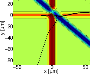
Figure 7: (Color online) Classical trajectories that illustrate two guiding breakdown mechanisms: escape by vibrational excitation (dashed line $v=1.5$ cm/s), and surmounting the barrier (solid line, $v=1.8$ cm/s). Laser parameters: $U=0.158$ $\mu$K; $U^{\prime}=0.474$ $\mu$K; $U_{b}=0.948$ $\mu$K; $w=w^{\prime}=w_{b}=5.7$ $\mu$m; $x_{0}=y_{0}=3$ $\mu$m and $\theta=45^{\circ}$.

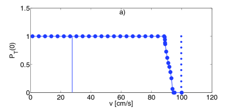
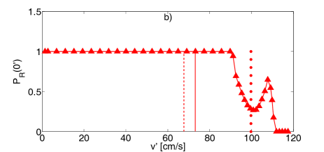
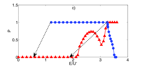
Figure 8: (Color online) (a,b,c): Same as in Fig. 6 for a different laser configuration. Laser parameters: $U=0.4$ mK; $U^{\prime}=2.8$ mK; $U_{b}=5.2$ mK; $w=w^{\prime}=1.03$ $\mu$m; $w_{b}=0.77$ $\mu$m; $x_{0}=y_{0}=0.41$ $\mu$m and $\theta=60^{\circ}$.

The potential asymmetry causes an asymmetry in the dynamics since, in general, for the same total energy, the probabilities $P_{0^{\prime}\to n}(E)$ and $P_{0\to n^{\prime}}(E)$ are quite different. This is compatible with time reversal invariance, which implies only the equality for probabilities of a process and the time reversed one. $P_{n\to{n^{\prime}}}(E)=P_{{n^{\prime}}\to n}(E)$ holds as long as no irreversible step takes place (that case will be considered in the following section). The nature of the stated asymmetry can be understood from the potential contour in Fig. 2c, or the 3D plot in Fig. 1. Even when the passage $n^{\prime}=0\to n=0$ ($0^{\prime}\to 0$ for short) is energetically allowed, a vibrationally unexcited atom does not find easily the lateral gate to the upper valley so, for a range of energies above the energy threshold (dashed vertical line in Figs. 6b and 8b), the atom is still reflected into the lower valley. This may be seen in Figs. 6b and 8b, where the reflection probability is shown for states beginning in the fundamental vibrational state $n^{\prime}=0$ of the lower valley for $\theta=45^{\circ}$ and $\theta=60^{\circ}$. The dynamical reflection is enhanced by increasing the angle $\theta$ so that the backward collision is more head-on, but increasing it too much may obstruct the passage in the forward direction at low velocities. Above the energies with full reflection, the atom with backward incidence may escape from the guides, when $V_{n^{\prime}}+K^{\prime}>U^{\prime}$, or surmount the potential barrier when $V_{n^{\prime}}+K^{\prime}>{U}_{b}$ (in this inequality we neglect the small effect of the upper valley potential). The corresponding energy thresholds for these processes are marked by solid and dotted lines in Figs. 6b and 8b but, as for forward motion, the effective thresholds occur at higher velocities.

V Diode effect

The stable plateaus for full transmission and reflection and the asymmetry for forward and backward motion from the ground transverse states are prerequisites for a diode but not enough. A diodic or “one-way” barrier effect is achieved by complementing these features with vibrational cooling in a region of the lower valley. Several cooling mechanisms have been demonstrated or proposed for neutral atoms in tight traps: Tuchendler et al. Tuch have cooled single ⁸⁷Rb atoms in the tight-confining directions of a strongly focused dipole trap with optical molasses; Sideband cooling has been demonstrated for alkali-earth atoms Katori03 using a “magic weavelenth” light-shift compensating technique Katori , and for Cs atoms by means of 2-photon Raman transitions in 1D Salomon , 2D Jessen , and 3D Chu far-detuned optical lattices; rf-induced Sisyphus cooling has been also realized for ⁸⁷Rb Wieman .

We shall not model in detail any of these methods here but simply assume that vibrational cooling is performed on the atoms that have been heated transversely in the forward passage and analyze the consequences for backward motion. In the ideal case of cooling down to the ground state, $n^{\prime}\to 0^{\prime}$, keeping the same kinetic energy $K^{\prime}$, the backward passage to the upper valley is energetically forbidden if $K^{\prime}+V_{0^{\prime}}<V_{0}+\Delta$, or using Eq. (6) and replacing $V_{n^{\prime}}$ by $\langle V^{\prime}\rangle$, $\langle V^{\prime}\rangle>K$ ($V_{0^{\prime}}$ is neglected). In fact it will not occur even at higher kinetic energies because of the 2D reflection effect described in the previous section. To determine if backward reflection is possible for a given incident $K$, we need the forward transmission and backward reflection velocity intervals of Figs. 6a,b or 8a,b (this has been combined in Figs. 6c and 8c, where the reflection information is represented by $1-P_{R}$), and the dependence $\langle V^{\prime}\rangle(K)$. After (perfect) vibrational cooling the backwards energy is

$$K^{\prime}+V_{0^{\prime}}=K+\Delta+V_{0}-\langle V^{\prime}\rangle+V_{0^{\prime}},$$ (8)

We may now check the value of $P_{R}(0^{\prime})$ for this energy to see if the atoms are reflected back into the lower valley. We have done this for the edge points of the total-transmission interval and the result is represented by the arrows in Figs. 6c and 8c. Note that for the 45^∘ case in Fig. 6c, the high velocity edge of full forward transmission does not correspond to backward reflection. This may be remedied by increasing the range of full reflection with a larger $\theta$ angle. For a lower valley as deep as the trap in Tuch and $\theta=60^{\circ}$, see Fig. 8c, a broad stable operating range for diodic behaviour is achieved, where the full range of forward passage corresponds, after transverse cooling, to full reflection in the backward direction.

VI Conclusions

Guided atom lasers in the ground state of the transverse confinement have been recently realized laser1 ; laser2 ; laser3 and more complicated settings are being considered, in particular with crossed beams, following similar developments in magnetic waveguides that may pave the way to new interferometers, atom integrated circuits and analogs of electronic devices atomtronics ; Holland09 .

In this work we have explored a realization of straight angle bends in asymmetrical optical waveguides for cold atoms, with two red and one blue detuned lasers, as well as the possibility to use the transverse heating caused by this geometry, combined with vibrational cooling, to implement a diodic (one-way) device. Indeed the transmission and reflection probabilities of the proposed structure offer the stability with respect to incident velocity required for an efficient diode. The different elements of the proposed device have been already implemented separately, and the remaining technical challenge is their combination into a single device.

Appendix A Classical dynamics

Classical trajectories are a useful tool to explore the effect of varying parameters faster than the quantum computation. They also provide physical insight. We solve Newton’s equations

$$m\ddot{x}=-\frac{\partial\tilde{U}(x,y)}{\partial x},\quad m\ddot{y}=-\frac{\partial\tilde{U}(x,y)}{\partial y},$$ (9)

where $\tilde{U}(x,y)=\tilde{U}+\tilde{U}^{\prime}+\tilde{U}_{b}$ are given in Eqs. (1, 2, 3), transformed into a system of four equations with a fourth-order Runge-Kutta method.

To mimic the scattering at fixed longitudinal and vibrational energies we consider an ensemble average set as follows: we take first a classical reference particle moving periodically in the transversal direction of the upper valley with the same transverse energy as the quantum state. To run an even number $N$ of trajectories the period of this reference particle is divided into $N$ equal time segments $[t_{i},t_{i+1}]$ and the $N$ values of $t_{i}$ set the initial transverse conditions for the trajectories of the ensemble. For the longitudinal motion we simply impart to the trajectories the longitudinal momentum $p$.

Appendix B Split-Operator Method (SOM)

Given the time dependent Schrödinger equation with Hamiltonian

$$\hat{H}=\frac{{\bf\hat{p}}^{2}}{2m}+{\bf\hat{U}}=\frac{\hat{p}_{x}^{2}+\hat{p}_{y}^{2}}{2m}+\tilde{U}(\hat{X},\hat{Y}),$$ (10)

the Split Operator Method (SOM) approximates the evolution operator as

$$e^{-it\left(\frac{{\bf\hat{p}}^{2}}{2m}+{\bf\hat{U}}\right)/\hbar}\approx e^{-it\left(\frac{{\bf\hat{p}}^{2}}{4m}\right)/\hbar}e^{-it{\bf\hat{U}}/\hbar}e^{-it\left(\frac{{\bf\hat{p}}^{2}}{4m}\right)/\hbar},$$ (11)

The resulting integrals are easily solved using the Fast Fourier Transform (FFT) technique rk .

B.1 Discretization and experimental setting

The validity of the discretization approximation requires rk ; ahj

$$\frac{Q_{x}}{n_{x}}<\frac{\Delta x}{L_{x}}<\frac{1}{4\pi Q_{x}}$$ (12)

$$p_{m,x}<\frac{\hbar\pi}{dx},$$ (13)

$$dt\ll\frac{\hbar}{T_{max}},\frac{\hbar}{U_{max}},$$ (14)

where $Q_{x}$ is a quality factor which takes into account the number of the lattice points that represent the wave function in coordinate and momentum representations, $L_{x}$ and $n_{x}$ are the lattice length, and the number of divisions, and $dx$ and $dt$ are the space and time steps. $\Delta x$ and $p_{m}$ are the minimal spatial dispersion (usually the one at $t=0$) and the maximum momentum value. Finally $U_{max}$ is the maximum potential energy and $K_{max}$ is the maximum kinetic energy during the simulation, $K_{max,x}<\frac{p_{m,x}^{2}}{2m}$. For the $y$-direction we have similar conditions. In all calculations we set $Q\geq 15$. Other parameters are $n_{x}=n_{y}=4096$.

B.2 Stationary transmission amplitudes from wavepacket computations

We write the transmitted wavepacket state as

$$\Psi_{T}(x,y,t) = \sum_{n^{\prime}}\int_{-\infty}^{\infty}\!\!dp\ v_{n^{\prime}}(x)e^{-iV_{n^{\prime}}t/\hbar}$$ (15)

$$\times T_{0n^{\prime}}(p)\frac{e^{-iq_{n^{\prime}}y/\hbar}}{\sqrt{h}}\phi(p)e^{-iq_{n^{\prime}}^{2}t/2m\hbar},$$

where $p$ is the incident, longitudinal momentum of the atoms in the upper valley, $q_{n^{\prime}}=[p^{2}+2m(V_{0}+\Delta-V_{n^{\prime}})]^{1/2}$ is the longitudinal momentum for the vibrational state $n^{\prime}$, $v_{n^{\prime}}(x)=\langle x|v_{n^{\prime}}\rangle$ is the amplitude of a lower valley vibrational state and $\phi(p)=\langle p|\psi(x,0)\rangle$ is the initial momentum distribution of the wave function given by Eq. (5). Finally the transmitted wave function is projected onto one particular eigenstate $v_{n^{\prime}}(x)$,

$$\langle v_{n^{\prime}}|\Psi_{T}(x,y,t)\rangle = \frac{1}{\sqrt{h}}\int_{-\infty}^{\infty}\!\!dp\ \Big{[}T_{0n^{\prime}}(p)\phi(p)$$ (16)

$$\times {e^{-iq_{n^{\prime}}y/\hbar}}e^{-it\left(\frac{q_{n^{\prime}}^{2}}{2m}+V_{n^{\prime}}\right)/\hbar}\Big{]}.$$

Defining the inverse Fourier transform as

$$\tilde{\omega}_{n^{\prime}}(E)=\frac{1}{\sqrt{h}}\int_{-\infty}^{\infty}\!\!dt\ \langle v_{n^{\prime}}|\Psi_{T}(x,y,t)\rangle e^{iEt/\hbar},$$ (17)

and integrating Eq. (16) with respect to time from $-\infty$ to $\infty$ (In practice $t=0$ plays the role of $t=-\infty$, whereas $t=\infty$ is approximated by the time when the tails of the transmitted wave function are not affected by the barrier.), we obtain

$$T_{0n^{\prime}}(p)=\frac{p}{m}\frac{e^{iy\sqrt{p^{2}+2m(\Delta+V_{0}-V_{n^{\prime}}})/\hbar}}{\phi(p)}\tilde{\omega}_{n^{\prime}}\!\!\left(\frac{p^{2}}{2m}+V_{0}+\Delta\right).$$ (18)

Its modulus squared times $q_{n^{\prime}}/p$ gives the transmittance (transmission probability) from the ground state of the upper channel to the $n^{\prime}$th-vibrational level of the lower guide.

References

- (1) J. Fortágh and C. Zimmermann, Rev. Mod. Phys. 79, 235 (2007).
- (2) R. Dumke, T. Müther, M. Volk, W. Ertmer, and G. Birkl, Phys. Rev. Lett. 89, 220402 (2002).
- (3) W. Guerin, J. F. Riou, J. P. Gaebler, V. Josse, P. Bouyer, and A. Aspect, Phys. Rev. Lett. 97 200402 (2006).
- (4) A. Couvert, M. Jeppesen, T. Kawalec, G. Reinaudi, R. Mathevet, and D. Guéry-Odelin, Europhys. Lett. 83 50001 (2008).
- (5) G. L. Gattobigio, A. Couvert, M. Jeppesen, R. Mathevet, and D. Guéry-Odelin, Phys. Rev. A 80 041605(R) (2009).
- (6) N. Blanchard and A. Zozulya, Opt. Commun. 190, 231 (2001).
- (7) P. Leboeuf and N. Pavloff, Phys. Rev. A 64, 033602 (2001).
- (8) W. Hänsel, P. Hommelhoff, T. W. Hänsch, and J. Reichel, Nature 413 498 (2001).
- (9) M. W. Bromley and B. D. Esry, Phys. Rev. A 68, 043609 (2003).
- (10) M. W. Bromley and B. D. Esry, Phys. Rev. A 69, 053620 (2004).
- (11) A. Ruschhaupt and J. G. Muga, Phys. Rev. A 70, 061604(R) (2004).
- (12) A. Ruschhaupt and J. G. Muga, Phys. Rev. A 73, 013608 (2006).
- (13) A. Ruschhaupt, J. G. Muga, and M. G. Raizen, J. Phys. B: At. Mol. Opt. Phys. 39, L133 (2006).
- (14) A. Ruschhaupt, J. G. Muga, and M. G. Raizen, J. Phys. B 39, 3833 (2006).
- (15) A. Ruschhaupt and J. G. Muga, Phys. Rev. A 76, 013619 (2007).
- (16) M. G. Raizen, A. M. Dudarev, Qian Niu, and N. J. Fisch, Phys. Rev. Lett. 94, 053003 (2005).
- (17) A. M. Dudarev, M. Marder, Qian Niu, N. J. Fisch, and M. G. Raizen, Europhysics Letters 70, 761 (2005).
- (18) G. N. Price, S. T. Bannerman, E. Narevicius, and M. G. Raizen, Laser Physics 17, 965 (2007).
- (19) G. N. Price, T. Bannerman, K. Viering, E. Narevicius, and M. G. Raizen, Phys. Rev. Lett. 100, 093004 (2008).
- (20) J. J. Thorn, E. A. Schoene, T. Li, and D. A. Steck, Phys. Rev. Lett. 100, 240407 (2008).
- (21) A. Ruschhaupt and J. G. Muga, J. Phys. B 41, 205503 (2008).
- (22) M. G. Raizen, Science 324, 1403 (2009)
- (23) J. J. Thorn, E. A. Schoene, T. Li, and D. A. Steck, Phys. Rev. A 79, 063402 (2009).
- (24) H. Kreutzmann, U. V. Poulsen, M. Lewenstein, R. Dumke, W. Ertmer, G. Birkl, and A. Sanpera Phys. Rev. Lett. 92, 163201 (2004).
- (25) M. D. Girardeau, Kunal K. Das, and E. M. Wright, Phys. Rev. Lett. 66, 023604 (2002).
- (26) O. Houde, D. Kadio, and L. Pruvost, Phys. Rev. Lett. 85, 5543 (2000).
- (27) D. J. Han, M. T. DePue, and D. S. Weiss, Phys. Rev. A 63, 023405 (2001).
- (28) C. Tuchendler, A. M. Lance, A. Browaeys, Y. R. Sortais, and P. Grangier, Phys. Rev. A 78, 033425 (2008).
- (29) T. Ido and H. Katori, Phys. Rev. Lett. 91, 053001 (2003).
- (30) H. Katori, T. Ido, and M. Kuwata-Gonokami, J. Phys. Soc. Japan 68, 2479 (1999).
- (31) H. Perrin, A. Kuhn, I. Bouchoule and C. Salomon, Europhys. Lett. 42 4, 395 (1998).
- (32) S. E. Hamann, D. L. Haycock, G. Klose, P. H. Pax, I. H. Deutsch, and P. S. Jessen, Phys. Rev. Lett. 80, 4149 (1998).
- (33) A. J. Kerman, V. Vuletic, C. Chin, and S. Chu, Phys. Rev. Lett. 84, 439 (2000).
- (34) K. W. Miller, S. Dürr, and C. Wieman, Phys. Rev. A 66, 023406 (2002).
- (35) B. T. Seaman, M. Krämer, D. Z. Anderson, and M. J. Holland Phys. Rev. A 75, 023615 (2007).
- (36) R. A. Pepino, J. Cooper, D. Z. Anderson, and M. J. Holland, Phys. Rev. Lett. 103, 140405 (2009).
- (37) R. Kosloff, J. Phys. Chem 92, 2087 (1988).
- (38) A. Goldberg, H. M. Schey and J. L. Schwartz, American J. Phys. 35, 3 (1967).