Boltzmann Samplers, Pólya Theory, and Cycle Pointing

Abstract.

We introduce a general method to count unlabeled combinatorial structures and to efficiently generate them at random. The approach is based on pointing unlabeled structures in an “unbiased” way that a structure of size $n$ gives rise to $n$ pointed structures. We extend Pólya theory to the corresponding pointing operator, and present a random sampling framework based on both the principles of Boltzmann sampling and on Pólya operators. All previously known unlabeled construction principles for Boltzmann samplers are special cases of our new results. Our method is illustrated on several examples: in each case, we provide enumerative results and efficient random samplers. The approach applies to unlabeled families of plane and nonplane unrooted trees, and tree-like structures in general, but also to families of graphs (such as cacti graphs and outerplanar graphs) and families of planar maps.

This is the extended and revised journal version of a conference paper with the title “An unbiased pointing operator for unlabeled structures, with applications to counting and sampling”, which appeared in the Proceedings of ACM-SIAM Symposium on Discrete Algorithms (SODA’07), 7-9 January 2007, New Orleans.

1. Introduction

Pointing (or rooting) is an important tool to derive decompositions of combinatorial structures, with many applications in enumerative combinatorics. Such decompositions can for instance be used in polynomial-time algorithms that sample structures of a combinatorial class uniformly at random. For a class of labeled structures, pointing corresponds to taking the derivative of the (typically exponential) generating function of the class. In other words, each structure of size $n$ gives rise to $n$ pointed (or rooted) structures. Other important operations on classes of combinatorial structures are the disjoint union, the product, and the substitution operation – they correspond to addition, multiplication, and composition of the associated generating functions. Together with the usual basic classes of combinatorial structures (finite classes, the class of finite sets, the class of finite sequences, and the class of cycles), this collection of constructions is a powerful device to define a great variety of combinatorial families.

If a class of structures can be described by recursive specifications involving pointing, disjoint unions, products, substitutions, and the basic classes, then the techniques of analytic combinatorics can be applied to obtain enumerative results, to study statistical properties of random structures in the class, and to derive efficient random samplers. An expository account for this line of research is [10]. Among recent developments in the area of random sampling are Boltzmann samplers [9], which are an attractive alternative to the recursive method of sampling [25, 11]. Both approaches provide in a systematic way polynomial-time uniform random generators for decomposable combinatorial classes. The advantage of Boltzmann samplers over the recursive method of sampling is that Boltzmann samplers operate in linear time if a small relative tolerance is allowed for the size of the output, and that they have a small preprocessing cost, which makes it possible to sample very large structures.

A third general random sampling approach is based on Markov chains. This approach does not require recursive decompositions of structures, and is applicable on a wide range of combinatorial classes. However, Markov chain methods are mostly limited to approximate uniformity. Moreover, it is usually difficult to obtain bounds on the rate of convergence to the uniform distribution [20].

All the results in this paper concern classes of unlabeled combinatorial structures, i.e., the structures are considered up to isomorphism. In the case of the class of all graphs, the labeled and the unlabeled model do not differ much, which is due to the fact that almost all graphs do not have a non-trivial automorphism (see e.g., [5, Ch. 9.] and [17]). However, for many interesting classes of combinatorial structures (and for most of the classes studied in this paper), the difference between the labeled and the unlabeled setting does matter.

The Markov chain approach can be adapted also to sample unlabeled structures approximately uniformly at random, based on the orbit counting lemma [19]. Again, the rate of convergence is usually very difficult to analyze, and frequently these Markov chains do not have a polynomial convergence rate [15]. For unlabeled structures, the approach faces additional difficulties: to computationally implement the transitions of the Markov chain, we have to be able to generate structures with a given symmetry uniformly at random (this is for instance a difficult task for planar graphs), and we have to be able to generate a symmetry of a given structure (for the class of all finite graphs, this task is computationally equivalent to the graph isomorphism problem).

To enumerate unlabeled structures, typically the ordinary generating functions are the appropriate tool. Disjoint unions and products for unlabeled structures then still correspond to addition and multiplication of the associated generating functions as for labeled cases. Boltzmann samplers for classes described by recursive specifications involving these operations have recently been developed in [13]. However, the substitution operation for unlabeled structures no longer corresponds to the composition of generating functions, due to the symmetries an unlabeled structure might have. This problem can be solved by Pólya theory, which uses the generalization of generating functions to cycle index sums to take care of potential symmetries. Pólya theory provides a computation rule for the cycle index sum associated to a substitution construction. The presence of symmetries leads to another problem with the pointing (or rooting) operator: the fundamental property that a structure of size $n$ gives rise to $n$ pointed structures does not hold. Indeed, if a structure of size $n$ has a non-trivial automorphism, then it corresponds to less than $n$ pointed structures (because pointing at two vertices in symmetric positions produces the same pointed structure). Thus, for unlabeled structures, the classical pointing operator does not correspond to the derivative of the ordinary generating function.

In this paper, we introduce an unbiased pointing operator for unlabeled structures. The operator is unbiased in the sense that a structure of size $n$ gives rise to $n$ pointed structures. It produces cycle-pointed structures, i.e., combinatorial structures $A$ together with a marked cyclic sequence of atoms of $A$ that is a cycle of an automorphism of $A$. Accordingly, we call our operator cycle-pointing. The idea is based on Parker’s lemma in permutation group theory [7] (this will be discussed in Remark 3.1). We develop techniques to apply this new pointing operator to enumeration and random sampling of unlabeled combinatorial classes. The crucial point is that cycle-pointing is unbiased. As a consequence, performing both tasks of enumeration and uniform random sampling on a combinatorial class is equivalent to performing these tasks on the associated cycle-pointed class.

To understand how we use our operator, it is instructive to look at the class of free trees, i.e., unrooted and nonplane trees (equivalently, acyclic connected graphs). Building on the work of Cayley and Pólya, Otter [26] determined the exact and asymptotic number of free trees. To this end, he developed the by-now standard dissimilarity characteristic equation, which relates the number of free trees with the number of rooted nonplane trees; see [16]. The best-known method to sample free trees uniformly at random is due to Wilf [34], and uses the concept of the centroid of a tree. The method is an example of application of the recursive method of sampling and requires a pre-processing step where a table of quadratic size is computed.

Cycle-pointing provides a new way to count and sample free trees. Both tasks are carried out on cycle-pointed (nonplane) trees. The advantage of studying cycle-pointed trees is that the pointed cycle provides a starting point for a recursive decomposition. In the case of cycle-pointed trees, we can formulate such a decomposition using standard constructions such as disjoint union, product, and substitution (which requires to suitably adapt these constructions to the cycle-pointed framework). We want to stress that, despite some superficial similarities, this method for counting free trees is fundamentally different from the previously existing methods mentioned above, and it proves particulary fruitful in the context of random generation. Indeed, the dissimilarity characteristic equation [26] and the dissymmetry theorem [2] both lead to generating function equations involving subtraction. However, subtraction yields massive rejection when translated into a random generator for the class of structures (both for Boltzmann samplers and for the recursive method). In contrast, the equations produced by the method based on cycle-pointing have only positive signs, and the existence of a Boltzmann sampler for (cycle-pointed) free trees, with no rejection involved, will follow directly from the general results derived in this paper. As usual, the Boltzmann samplers we obtain have a running time that is linear in the size of the structure generated, and have small pre-processing cost.

Similarly, we can decompose plane and nonplane trees, and more generally all sorts of tree-like structures. By the observation that the block decomposition of a graph has also a tree-like structure, we can apply the method to classes of graphs where the two-connected components can be explicitly enumerated. This leads to efficient Boltzmann samplers, for instance, for cacti graphs and outerplanar graphs, improving on the generators of [4]. Further, our strategy is not limited to only tree-like structures, but can also be applied to other classes of structures that allow for a recursive decomposition. To demonstrate this, we sketch how the method can be applied to count and sample certain classes of planar maps.

Outline of the paper

To formalize our general results on enumeration and sampling for classes of unlabeled combinatorial structures in full generality, we apply the concept of combinatorial species; we recall this concept in Section 2. In Section 3 we introduce cycle-pointed species and the cycle-pointing operator. Section 4 is devoted to applications of our cycle-pointing operator in enumeration. The technique in which we use the operator to obtain recursive decomposition strategies for unlabeled enumeration is very generally applicable; we illustrate it by the enumeration of (unrooted) non-plane and plane trees, cacti graphs, and maps. Finally, in Section 5, we present how to apply the concepts introduced in this paper to obtain highly efficient random sampling procedures for unlabeled structures. This is illustrated by applications for sampling of concrete and fundamental classes of unlabeled combinatorial structures; several of these concrete sampling results are either new or improve the state-of-the-art of sampling efficiency.

2. Preliminaries

In this paper we work with classes of combinatorial structures, such as graphs, relational structures, functions, trees, plane trees, maps, words, terms, or permutations. There are many ways to define formally these objects; for example, rooted trees can be coded as special types of directed graphs, but also as terms. Which formal representation of a combinatorial structure is best usually depends on the application.

When we are interested in combinatorial enumeration, the differences in representation are not essential; in the example above, we have the same number of rooted trees, no matter how they are represented. We would thus like to have a formalism that is sufficiently abstract so that our results apply to broad classes of combinatorial structures. At the same time, we would like to have a formalism for classes of combinatorial structures that supports fundamental construction operations for combinatorial classes, such as formation of disjoint unions, products, and substitution, and allows to state general results about enumeration and random sampling.

The theory of combinatorial species is an elegant tool that fully satisfies the needs mentioned above. We give a brief introduction to species, and refer to Bergeron, Labelle, and Leroux [2] for a broader treatment of the topic. The fundamental and well-known classes of combinatorial structures that we treat in Section 4 provide ample illustration of the concepts we define in this section.

2.1. Combinatorial Species

We closely follow the presentation in [2]. A species of structures is a functor $\mathcal{A}$ from finite sets $U$ to finite sets $\mathcal{A}[U]$, together with a rule that produces for each bijection $\sigma:U\rightarrow V$ a function from $\mathcal{A}[U]$ to $\mathcal{A}[V]$. Slightly abusing notation, this function will also be denoted by $\mathcal{A}[\sigma]$. The functions $\mathcal{A}[\sigma]$ must satisfy the following two (functorial) properties:

• for all bijections $\sigma:U\rightarrow V$ and $\tau:V\rightarrow W$,

  $$\mathcal{A}[\tau\circ\sigma]=\mathcal{A}[\tau]\circ\mathcal{A}[\sigma]\;;$$

• for the identity map $\text{Id}_{U}:U\rightarrow U$,

  $$\mathcal{A}[\text{Id}_{U}]=\text{Id}_{\mathcal{A}[U]}\;.$$

An element $A\in\mathcal{A}[U]$ is called an $\mathcal{A}$-structure on $U$. The elements of $U$ are called the atoms of $\mathcal{A}[U]$, and we refer to $|U|$ as the size of $A$. The function $\mathcal{A}[\sigma]$ is called the transport of $\mathcal{A}$-structures along $\sigma$. We write $\sigma\boldsymbol{\cdot}A$ for $\mathcal{A}[\sigma](A)$.

Definition 2.1.

Let $A_{1}\in\mathcal{A}[U]$ and $A_{2}\in\mathcal{A}[V]$ be two $A$-structures. A bijection $\sigma:U\rightarrow V$ is called an isomorphism from $A_{1}$ to $A_{2}$ if $A_{2}=\sigma\boldsymbol{\cdot}A_{1}=\mathcal{A}[\sigma](A_{1})$. An isomorphism from $A_{1}$ to $A_{1}$ is called an automorphism of $A_{1}$.

The advantage of species is that the rule $\mathcal{A}$ that produces the structures $\mathcal{A}[U]$ and the transport functions $\mathcal{A}[\sigma]$ can be described in any way; the book [2] gives instructive examples where this description is by axiomatic systems, explicit constructions, algorithms, combinatorial operations, or functional equations.

Definition 2.2.

A species $\mathcal{A}$ is a subspecies of a species $\mathcal{B}$ (and we write $\mathcal{A}\subseteq\mathcal{B}$) if it satisfies the following two conditions:

• for any finite set $U$, $\mathcal{A}[U]\subseteq\mathcal{B}[U]$;

• for any $\sigma:U\rightarrow V$ we have $\mathcal{A}[\sigma]=\mathcal{B}[\sigma]|_{\mathcal{B}[U]}$.

2.2. Enumeration

For all finite sets $U$, the number of $\mathcal{A}$-structures on $U$ depends only on the number of elements of $U$ (and not on the elements of $U$). If $\mathcal{A}$ is a species, we write $a_{n}$ for $|\mathcal{A}[\{1,\dots,n\}]|$, the cardinality of the set of $\mathcal{A}$-structures on $\{1,\dots,n\}$. The series

$$\mathcal{A}(x):=\sum_{n\geq 0}\frac{1}{n!}a_{n}x^{n}$$ (1)

is called the exponential generating series of the species $\mathcal{A}$.

In this article we focus on unlabeled structures, i.e., we consider structures up to isomorphism. We may restrict ourselves to structures on sets of the form $U=[1..n]:=\{1,\dots,n\}$, and write $\mathcal{A}[n]$ for $\mathcal{A}[\{1,\dots,n\}]$. We define the equivalence relation $\sim$ on $\mathcal{A}[n]$ by setting $A_{1}\sim A_{2}$, for $A_{1},A_{2}\in\mathcal{A}[n]$, if and only if there is an isomorphism $\sigma:[1..n]\rightarrow[1..n]$ from $A_{1}$ to $A_{2}$. We also say that $A_{1}$ and $A_{2}$ have the same isomorphism type, and the equivalence classes of $\mathcal{A}$-structures on $[1..n]$ with respect to $\sim$ are also called unlabeled $\mathcal{A}$-structures of size $n$, The set of all those equivalence classes is denoted by $\widetilde{\mathcal{A}}_{n}$, and we write $\widetilde{a}_{n}$ for its cardinality $|\widetilde{\mathcal{A}}_{n}|$. The series

$$\widetilde{\mathcal{A}}(x):=\sum_{n\geq 0}\widetilde{a}_{n}x^{n}$$ (2)

is called the ordinary generating series (OGS) of $\mathcal{A}$. We use the classical notation $[x^{n}]\widetilde{\mathcal{A}}(x)$ to denote the $n$-th coefficient $\widetilde{a}_{n}$ in the power series $\widetilde{\mathcal{A}}(x)$.

2.3. Cycle index sums

For a species $\mathcal{A}$ and each $n\geq 0$, a symmetry of $\mathcal{A}$ of size $n$ is a pair $(A,\sigma)$ where $A$ is from $\mathcal{A}[n]$ and $\sigma$ is an automorphism of $A$. We call $A$ the underlying structure of the symmetry $(A,\sigma)$. Notice that the automorphism $\sigma$ can be the identity. We denote by $\mathrm{Sym}(\mathcal{A})$ the species defined by

$$\mathrm{Sym}(\mathcal{A})[n]:=\{(A,\sigma)\;|\;A\in\mathcal{A}[n]\text{ and $\sigma$ is an automorphism of $A$}\}\;.$$

The definition of the transport of $\mathrm{Sym}(\mathcal{A})$ is obvious (the definition of symmetries as an auxiliary species is standard; see Section 4.3 in  [2]). The weight-monomial of a symmetry $(A,\sigma)$ of size $n$ is defined as

$$w_{(A,\sigma)}:=\frac{1}{n!}\prod_{i=1}^{n}s_{i}^{c_{i}(\sigma)},$$ (3)

where, for $i\in[1..n]$, $s_{i}$ is a formal variable and $c_{i}(\sigma)$ is the number of cycles of $\sigma$ of length $i$. For simplicity, in the following we will write $c_{i}$ for $c_{i}(\sigma)$ if the corresponding automorphism is clear from the context. The cycle index sum of $\mathcal{A}$, denoted by $Z_{\mathcal{A}}(s_{1},s_{2},\ldots)$, or shortly $Z_{\mathcal{A}}$, is the formal power series defined as the sum of the weight-monomials over all the symmetries of $\mathcal{A}$,

$$Z_{\mathcal{A}}(s_{1},s_{2},\ldots):=\sum_{n\geq 0}\left(\sum_{(A,\sigma)\in\mathrm{Sym}(\mathcal{A})[n]}w_{(A,\sigma)}\right).$$ (4)

Cycle index sums for classes of combinatorial structures have been introduced by Pólya [28]. The following fact, which is based on Burnside’s lemma, shows that cycle index sums are a refinement of ordinary generating series.

Lemma 1 (Pólya).

Let $\mathcal{A}$ be a species of structures. For $n\geq 0$, each unlabeled structure $\tilde{A}\in\widetilde{\mathcal{A}}_{n}$ gives rise to $n!$ symmetries, i.e., there are $n!$ symmetries $(A,\sigma)$ such that $A\in\tilde{A}$. Hence,

$$Z_{\mathcal{A}}(x,x^{2},x^{3},\ldots)=\widetilde{\mathcal{A}}(x).$$ (5)

In the proofs of combinatorial identities it will be convenient to identify species that are essentially the same.

Definition 2.3.

Let $\mathcal{A}$ and $\mathcal{B}$ be two species. An isomorphism from $\mathcal{A}$ to $\mathcal{B}$ is a family of bijections $\alpha_{U}:\mathcal{A}[U]\rightarrow\mathcal{B}[U]$ which satisfies the following naturality condition: for any bijection $\sigma:U\rightarrow V$ between two finite sets $U$ and $V$, and for any $\mathcal{A}$-structure $A$ on $U$, one must have

$$\sigma\boldsymbol{\cdot}\alpha_{U}(A)=\alpha_{V}(\sigma\boldsymbol{\cdot}A)\;.$$

It is known (see [2]) that when $\mathcal{A}$ is isomorphic to $\mathcal{B}$, then $\mathcal{A}(x)=\mathcal{B}(x)$, $\widetilde{\mathcal{A}}(x)=\widetilde{\mathcal{B}}(x)$, and $Z_{\mathcal{A}}(x_{1},x_{2},\dots)=Z_{\mathcal{B}}(x_{1},x_{2},\dots)$. Hence, for the purposes of combinatorial enumeration we can even identify isomorphic species, and as in [2] we write $\mathcal{A}=\mathcal{B}$ when $\mathcal{A}$ and $\mathcal{B}$ are isomorphic species.

2.4. Basic species and combinatorial constructions

We now recall a collection of basic species and combinatorial constructions. We start with the description of some basic species, and then introduce the three fundamental constructions of disjoint union, product, and substitution.

Basic species	Notation	Cycle index sum
Empty species	0	$\displaystyle Z_{\mathbf{0}}=0$
Neutral species	1	$\displaystyle Z_{\mathbf{1}}=1$
Atomic species	$X$	$\displaystyle Z_{X}=s_{1}$
Sequences with $k$ atoms	$\textsc{Seq}^{[k]}$	$\displaystyle Z_{\textsc{Seq}^{[k]}}=s_{1}^{k}$
Sets with $k$ atoms	$\textsc{Set}^{[k]}$	$\displaystyle Z_{\textsc{Set}^{[k]}}=[x^{k}]\exp\Big{(}\sum_{r\geq 1}\frac{1}{r}x^{r}s_{r}\Big{)}$
Cycles with $k$ atoms	$\textsc{Cyc}^{[k]}$	$\displaystyle Z_{\textsc{Cyc}^{[k]}}=\frac{1}{k}\sum_{r|k}\phi(r)s_{r}^{k/r}$
Species of sequences	Seq	$\displaystyle Z_{\textsc{Seq}}=\frac{1}{1-s_{1}}$
Species of sets	Set	$\displaystyle Z_{\textsc{Set}}=\exp\Big{(}\sum_{r\geq 1}\frac{1}{r}s_{r}\Big{)}$
Species of cycles	Cyc	$\displaystyle Z_{\textsc{Cyc}}=1+\sum_{r\geq 1}\frac{\phi(r)}{r}\log\left(\frac{1}{1-s_{r}}\right)$
Construction	Notation	Cycle index sum
Union of two species	$\mathcal{M}=\mathcal{A}+\mathcal{B}$	$\displaystyle Z_{\mathcal{M}}=Z_{\mathcal{A}}+Z_{\mathcal{B}}$
Product of two species	$\mathcal{M}=\mathcal{A}\boldsymbol{\cdot}\mathcal{B}$	$\displaystyle Z_{\mathcal{M}}=Z_{\mathcal{A}}\boldsymbol{\cdot}Z_{\mathcal{B}}$
Composition of two species	$\mathcal{M}=\mathcal{A}\circ\mathcal{B}$	$\displaystyle Z_{\mathcal{M}}=Z_{\mathcal{A}}\circ Z_{\mathcal{B}}$

Figure 1. The cycle index sums of basic species and of species composed by $+$, $\boldsymbol{\cdot}$, and $\circ$.

2.4.1. Basic Species.

The most elementary species are

• the empty species ${\bf 0}$ defined by ${\bf 0}[U]:=\emptyset$ for all $U$;

• the neutral species ${\bf 1}$ defined by ${\bf 1}[U]:=\{\emptyset\}$ if $|U|=0$ and ${\bf 1}[U]:=\emptyset$ otherwise;

• the atomic species $X$ defined by $X[U]:=\{U\}$ if $|U|=1$ and $X[U]:=\emptyset$ otherwise;

• the species of sets Set defined by $\textsc{Set}[U]:=\{U\}$;

• the species Seq of sequences defined by $\textsc{Seq}[U]:=\{(U,<)\;|\;U\text{ is linearly ordered by }<\}$;

• the species Cyc of oriented cycles (or cyclic permutations) defined by

  $$\textsc{Cyc}[U]:=\{(U,\pi)\;|\;\pi\text{ is a cyclic permutation of }U\}\;.$$

In each case, the definition of the transport $\mathcal{A}[\sigma]$ of $\mathcal{A}$-structures is obvious.

If $\mathfrak{A}$ is a species, then $\mathfrak{A}^{[n]}$ denotes the species defined by $\mathcal{A}^{[n]}[U]:=\mathcal{A}[U]$ if $|U|=n$ and $\mathcal{A}[U]:=\emptyset$ otherwise. The transport $\mathcal{A}^{[n]}[\sigma]$ for bijections $\sigma:U\rightarrow V$ is defined by $\mathcal{A}^{[n]}[\sigma]:=\mathcal{A}[\sigma]$ if $|U|=n$ and $\mathcal{A}^{[n]}[\sigma]:=\text{Id}_{\mathcal{A}[U]}$ otherwise. In particular, $X$ is $\textsc{Set}^{[1]}$.

2.4.2. Constructions

We now describe the three fundamental constructions that we use to construct species from other species.

Disjoint union. For two species $\mathcal{A}$ and $\mathcal{B}$, the species $\mathcal{A}+\mathcal{B}$, called the disjoint union (or sum) of $\mathcal{A}$ and $\mathcal{B}$, is defined by $(\mathcal{A}+\mathcal{B})[U]=(\{1\}\times\mathcal{A}[U])\cup(\{2\}\times\mathcal{B}[U])$. The transport along a bijection $\sigma:U\rightarrow V$ is carried out by setting, for any $(\mathcal{A}+\mathcal{B})$-structure $C$ on $U$,

$$(\mathcal{A}+\mathcal{B})[\sigma]((i,C)):=\left\{\begin{array}[]{rl}\mathcal{A}[\sigma](C)&\text{ if }i=1\\ \mathcal{B}[\sigma](C)&\text{ if }i=2\;.\end{array}\right.$$

Note that when $\mathcal{A},\mathcal{A}^{\prime},\mathcal{B},\mathcal{B}^{\prime}$ are species such that $\mathcal{A}=\mathcal{A}^{\prime}$ (i.e., $\mathcal{A}$ and $\mathcal{A}^{\prime}$ are isomorphic) and $\mathcal{B}=\mathcal{B}^{\prime}$, then $\mathcal{A}+\mathcal{B}=\mathcal{A}^{\prime}+\mathcal{B}^{\prime}$.

The disjoint union of a countably infinite sequence $\mathcal{A}_{1},\mathcal{A}_{2},\dots$ of species is defined analogously, setting $\big{(}\sum_{i\geq 1}\mathcal{A}_{i}\big{)}[U]:=\bigcup_{i\geq 1}(i,\mathcal{A}_{i}[U])$ (this species is well-defined provided the set on the right is finite for each finite set $U$).

Product. The cartesian (often also called partitional or dinary) product $\mathcal{A}\boldsymbol{\cdot}\mathcal{B}$ of two species $\mathcal{A}$ and $\mathcal{B}$ is the species defined as follows. An $(\mathcal{A}\boldsymbol{\cdot}\mathcal{B})$-structure on $U$ is an ordered pair $C=(A,B)$ where $A$ is an $\mathcal{A}$-structure on a set $U_{1}\subseteq U$, $B$ is a $\mathcal{B}$-structure on a set $U_{2}\subseteq U$, $U_{1}\cap U_{2}=\emptyset$, and $U_{1}\cup U_{2}=U$. The transport along a bijection $\sigma:U\rightarrow V$ is carried out by setting, for each $(\mathcal{A}\boldsymbol{\cdot}\mathcal{B})$-structure $C=(A,B)$ on $U$,

$$(\mathcal{A}\boldsymbol{\cdot}\mathcal{B})[\sigma](C):=(\mathcal{A}[\sigma_{1}](A),\mathcal{B}[\sigma_{2}](B))$$

where $\sigma_{i}$ is the restriction $\sigma|_{U_{i}}$ of $\sigma$ on $U_{i}$ for $i\in\{1,2\}$.

Again we note that when $\mathcal{A},\mathcal{A}^{\prime},\mathcal{B},\mathcal{B}^{\prime}$ are species such that $\mathcal{A}=\mathcal{A}^{\prime}$ and $\mathcal{B}=\mathcal{B}^{\prime}$, then $\mathcal{A}\boldsymbol{\cdot}\mathcal{B}=\mathcal{A}^{\prime}\boldsymbol{\cdot}\mathcal{B}^{\prime}$.

Substitution. Given two species $\mathcal{A}$ and $\mathcal{B}$ such that $\mathcal{B}[\emptyset]=\emptyset$, the (partitional) composite of $\mathcal{B}$ in $\mathcal{A}$, denoted by $\mathcal{A}\circ\mathcal{B}$, is the species $\mathcal{C}$ obtained as follows. A $\mathcal{C}$-structure on $U$ is a triple $(\pi,A,B)$ where

• $\pi$ is a partition of $U$;

• $A$ is an $\mathcal{A}$-structure on the set of classes of $\pi$;

• $B:=(B_{p})_{p\in\pi}$ where for each class $p$ of $\pi$, $B_{p}$ is a $\mathcal{B}$-structure on $p$.

The transport along a bijection $\sigma:U\rightarrow V$ is carried out by setting, for any $\mathcal{C}$-structure $C=(\pi,A,(B_{p})_{p\in\pi})$ on $U$

$$\mathcal{C}[\sigma](C):=(\bar{\pi},\bar{A},(\bar{B}_{\bar{p}})_{\bar{p}\in\bar{\pi}})$$

where

• $\bar{\pi}$ is the partition of $V$ obtained by transport of $\pi$ along $\sigma$;

• the structure $\bar{A}$ is obtained from the structure $A$ by $\mathcal{A}$-transport along the bijection $\bar{\sigma}:\pi\rightarrow\bar{\pi}$ induced by $\sigma$ on $\pi$;

• for each $\bar{p}=\sigma(p)\in\bar{\pi}$, the structure $\bar{B}_{\bar{p}}$ is obtained from the structure $B_{p}$ by $\mathcal{B}$-transport along $\sigma|_{p}$.

We call the $\mathcal{A}$-structure $A$ the core of $(\pi,A,B)$, and $B_{p}$ in $B=(B_{p})_{p\in\pi}$ a component of $(\pi,A,B)$. Also for the substitution construction, we have that when $\mathcal{A},\mathcal{A}^{\prime},\mathcal{B},\mathcal{B}^{\prime}$ are species such that $\mathcal{A}=\mathcal{A}^{\prime}$ and $\mathcal{B}=\mathcal{B}^{\prime}$, then $\mathcal{A}\circ\mathcal{B}=\mathcal{A}^{\prime}\circ\mathcal{B}^{\prime}$.

Together with the basic species, these constructions provide an extremely powerful device for the description of combinatorial families. The substitution construction is particularly interesting, as it allows us to express other combinatorial constructions, such as the formation of sequences, sets, and cycles of structures of a species $\mathcal{A}$, which are specified as $\textsc{Seq}\circ\mathcal{A}$, $\textsc{Set}\circ\mathcal{A}$, and $\textsc{Cyc}\circ\mathcal{A}$, respectively.

As usual, and to avoid clumsy expressions with many brackets, we make the convention that in expressions involving several of the symbols $+,\boldsymbol{\cdot},\circ$, the symbol $\circ$ binds stronger than the symbol $\boldsymbol{\cdot}$, and the symbol $\boldsymbol{\cdot}$ binds stronger than the symbol $+$.

There are explicit rules to compute the cycle index sum for the basic species and for each construction.

Definition 2.4.

Given two power series $f:=f(x_{1},x_{2},x_{3}\ldots)$ and $g:=g(x_{1},x_{2},x_{3},\ldots)$ such that $g(0,0,\ldots)=0$, the plethystic composition of $f$ and $g$, as defined in [2], is the power series

$$f\circ g:=f(g_{1},g_{2},g_{3},\ldots),\ \ \ \mathrm{with}\ g_{k}=g(x_{k},x_{2k},x_{3k},\ldots)\;.$$ (6)

In other words, $f\circ g$ is the series $f$ where each variable $x_{k}$ is replaced by $g(x_{k},x_{2k},x_{3k},\ldots)$.

Proposition 2 (Pólya, Bergeron et al. [2]).

For each of the basic species $\{\mathbf{0},\mathbf{1}$, $X$, $\textsc{Seq}^{[k]}$, $\textsc{Set}^{[k]}$, $\textsc{Cyc}^{[k]}$, Seq, Set, $\textsc{Cyc}\}$, the associated cycle index sum has an explicit expression, as given in Figure 1. For each of the fundamental constructions $\wedge\in\{+,\boldsymbol{\cdot},\circ\}$, there is an explicit rule to compute the cycle index sum of the species $\mathcal{A}\wedge\mathcal{B}$, as given in Figure 1.

Remark 2.1.

The ordinary generating series of a species can be obtained from the cycle index sums for the species. For the sum and product constructions, we obtain

$$\mathcal{C}=\mathcal{A}+\mathcal{B} \Rightarrow \widetilde{\mathcal{C}}(x)=\widetilde{\mathcal{A}}(x)+\widetilde{\mathcal{B}}(x),$$ (7)

$$\mathcal{C}=\mathcal{A}\boldsymbol{\cdot}\mathcal{B} \Rightarrow \widetilde{\mathcal{C}}(x)=\widetilde{\mathcal{A}}(x)\cdot\widetilde{\mathcal{B}}(x).$$ (8)

For the substitution construction, the computation rule is

$$\hskip 28.45274pt\mathcal{C}=\mathcal{A}\circ\mathcal{B} \Rightarrow \widetilde{\mathcal{C}}(x)=Z_{\mathcal{A}}(\widetilde{\mathcal{B}}(x),\widetilde{\mathcal{B}}(x^{2}),\widetilde{\mathcal{B}}(x^{3}),\ldots).$$ (9)

2.5. Recursive Specifications.

It is possible to define species via recursive specifications that involve the fundamental constructions introduced above.

Definition 2.5.

A (standard) recursive specification with variables $x_{1},\dots,x_{m}$ over the species $\mathcal{A}_{1},\dots,\mathcal{A}_{\ell}$ is a system $\Psi$ of equations $x_{1}=e_{1},\dots,x_{m}=e_{m}$ where each $e_{i}$ is

• of the form $a+b$ or $a\boldsymbol{\cdot}b$ with $a,b\in\{x_{1},\ldots,x_{m},\mathcal{A}_{1},\dots,\mathcal{A}_{\ell}\}$, or

• of the form $a\circ b$ with $a\in\{\mathcal{A}_{1},\dots,\mathcal{A}_{\ell}\}$ and $b\in\{x_{1},\dots,x_{m},\mathcal{A}_{1},\dots,\mathcal{A}_{\ell}\}$.

Under a certain condition, a recursive specification $\Psi$ with variables $x_{1},\dots,x_{m}$ defines new species $\mathcal{X}_{1},\dots,\mathcal{X}_{m}$ as follows. We first define for each $i\geq 0$ a vector of species $\mathcal{X}_{1}^{(i)},\dots,\mathcal{X}_{m}^{(i)}$. For $i=1$, we set $(\mathcal{X}_{1}^{(i)},\dots,\mathcal{X}_{m}^{(i)})=({\bf 0},\dots,{\bf 0})$. For $i>1$ and $1\leq j\leq m$, the species $\mathcal{X}^{(i)}_{j}$ is defined from $e_{j}$ by substituting for all $1\leq k\leq m$ the occurrences of $x_{k}$ in $e_{j}$ by $\mathcal{X}_{k}^{(i-1)}$. The resulting expression only contains species and symbols $+$, $\boldsymbol{\cdot}$, and $\circ$, and hence evaluates to a species, unless $e_{j}=a\circ b$ and $b$ is substituted by a species that contains structures of size $0$. If this case never occurs, i.e., if $\mathcal{B}[\emptyset]=\emptyset$ whenever a species $\mathcal{B}$ is substituted for $b$ in an expression $a\circ b$, then we call $\Psi$ admissible.

Note that the sequence $\mathcal{X}_{k}^{(1)},\mathcal{X}_{k}^{(2)},\dots$ is monotone, that is, $\mathcal{X}_{k}^{(i)}\subseteq\mathcal{X}_{k}^{(i+1)}$ for all $1\leq k\leq m$ and all $i\geq 1$; this follows from the following basic fact (we omit the proof which is straightforward).

Proposition 3.

If $\mathcal{A},\mathcal{A}^{\prime},\mathcal{B},\mathcal{B}^{\prime}$ are species, and $\mathcal{A}\subseteq\mathcal{A}^{\prime}$, $\mathcal{B}\subseteq\mathcal{B}^{\prime}$, then $\mathcal{A}+\mathcal{B}\subseteq\mathcal{A}^{\prime}+\mathcal{B}^{\prime}$, $\mathcal{A}\boldsymbol{\cdot}\mathcal{B}\subseteq\mathcal{A}^{\prime}\boldsymbol{\cdot}\mathcal{B}^{\prime}$, and $\mathcal{A}\circ\mathcal{B}\subseteq\mathcal{A}^{\prime}\circ\mathcal{B}^{\prime}$.

Note that due to this proposition, it is easy to decide for a given recursive specification whether or not it is admissible (given also the information which of the species $\mathcal{A}_{1},\dots,\mathcal{A}_{\ell}$ contains structures of size $0$).

Definition 2.6.

Let $\Psi$ be an admissible recursive specification with variables $x_{1},\dots,x_{m}$ over the species $\mathcal{A}_{1},\dots,\mathcal{A}_{\ell}$, and let the species $\mathcal{X}^{(i)}_{j}$ be as described above. If for each $n$, the set $\bigcup_{i\geq 1}\mathcal{X}^{(i)}[n]$ is finite, then the species $\mathcal{X}_{1},\dots,\mathcal{X}_{m}$ specified by $\Psi$ are defined as follows. We set $\mathcal{X}_{j}[n]=\bigcup_{i\geq 1}\mathcal{X}_{j}^{(i)}[n]$. By monotonicity, for each $n$ we have that $\mathcal{X}_{j}[n]$ equals $\mathcal{X}_{j}^{(k)}[n]$ for some $k$, and so we can define the transport of $\mathcal{X}_{j}$ by $\mathcal{X}_{j}[\sigma]=\mathcal{X}_{j}^{(k)}[\sigma]$.

Definition 2.7.

Let $\mathfrak{A}$ be a class of species. The class of species that is decomposable over $\mathfrak{A}$ is the smallest class of species $\mathfrak{B}$ that contains $\mathfrak{A}$, and that contains all species that can be defined by recursive specifications over species from $\mathfrak{B}$.

2.6. Decomposition of symmetries

In this subsection we provide a proof of Proposition 2. The proof relies on a precise description of the nature of the automorphisms for the basic species and for the species obtained from one of the constructions $+$, $\boldsymbol{\cdot}$, or $\circ$. Even though proofs and details can already be found in [2], we give our own presentation here since we build on this later on, in particular to define random generation rules (Section 5).

2.6.1. Automorphisms of some basic species.

By convention, the neutral species $\bf{1}$ has the cycle-index sum $1$ (the structure of size $0$ is assumed to be fixed by the “empty” automorphism, of weight $1$).

The cycle index sum of $X$ is $s_{1}$. The only $X$-structures are over $U$ with $|U|=1$, and all automorphisms of such structures consist of a single cycle that has weight $s_{1}$.

For the species Seq, the only automorphisms are the identity, and the identity has weight $s_{1}^{k}/k!$. As there are $k!$ sequences of length $k$, the cycle index sum of $\textsc{Seq}^{[k]}$ is $s_{1}^{k}$. Since $\textsc{Seq}=\sum_{k\geq 0}\textsc{Seq}^{[k]}$, the cycle index sum for Seq is

$$Z_{\textsc{Seq}}=\sum_{k\geq 0}s_{1}^{k}=\frac{1}{1-s_{1}}.$$ (10)

For the species Cyc, the automorphisms are exactly the ‘shifts’: for a cycle $(v_{1},\ldots,v_{k})$, the shift of this cycle by $m\in[0..k-1]$ maps $v_{i}$ to $v_{i+m}$ where the indices are modulo $k$. The automorphisms consist of $k/r$ cycles of length $r$, where $r$ is the order of $m$ in $\mathbb{Z}/(k\mathbb{Z})$. For each divisor $r$ of $k$, there are $\phi(r)$ elements of order $r$ in $\mathbb{Z}/(k\mathbb{Z})$, where $\phi(.)$ is the Euler totient function. Hence, for each cycle of length $k$, the sum of the weight-monomials over all the cycles of size $r$ is $\phi(r)s_{r}^{k/r}/k!$, and the sum of the weight-monomials over all the symmetries is $\sum_{r|k}\phi(r)s_{r}^{k/r}/k!$. As there are $(k-1)!$ cycles of length $k$, the cycle index sum of $\textsc{Cyc}^{[k]}$ is $1/k\cdot\sum_{r|k}\phi(r)s_{r}^{k/r}$. For the species $\textsc{Cyc}=\sum_{k\geq 1}\textsc{Cyc}^{[k]}$ of all cycles, the sum of the weight-monomials over all symmetries of size $r$, which we denote by $Z_{{\textsc{Cyc}},r}$, is thus

$$Z_{{\textsc{Cyc}},r}=\sum_{k,r|k}\frac{\phi(r)}{k}s_{r}^{k/r}=\frac{\phi(r)}{r}\sum_{m\geq 1}\frac{1}{m}s_{r}^{m}=\frac{\phi(r)}{r}\log\left(\frac{1}{1-s_{r}}\right).$$ (11)

Therefore, summing $Z_{\textsc{Cyc},r}$ over $r\geq 1$, one obtains the expression of $Z_{\textsc{Cyc}}$ given in Figure 1.

For the species Set, the automorphisms are all permutations. Hence, the cycle index sum for Set is simply the exponential generating series for all permutations, where each cycle of length $i$ is marked by a variable $s_{i}$. In other words, when $f(x)$ denotes the exponential generating series for permutations, and $f(x;s_{1},s_{2},s_{3},\ldots)$ denotes the same generating series where each variable $s_{i}$ marks the number of cycles of length $i$, then the rules for computing exponential generating series yield

$$f(x;s_{1},s_{2},s_{3},\ldots)=\exp\left(\sum_{i\geq 1}\frac{1}{i!}x^{i}(i-1)!s_{i}\right)=\exp\left(\sum_{i\geq 1}\frac{1}{i}x^{i}s_{i}\right)\;.$$ (12)

Hence, $f(1;s_{1},s_{2},s_{3},\ldots)$ is the cycle index sum for Set, and the cycle index sum for $\textsc{Set}^{[k]}$ is $[x^{k}]f(x;s_{1},s_{2},s_{3},\ldots)$, which corresponds to a restriction to permutations of size $k$. Notice that $Z_{\textsc{Set}^{[k]}}$ is always a polynomial; for instance, we have

$$Z_{\textsc{Set}^{[2]}}=\frac{1}{2}(s_{1}^{2}+s_{2}),\ \ Z_{\textsc{Set}^{[3]}}=\frac{1}{6}(s_{1}^{3}+3s_{2}s_{1}+2s_{3}),\ \ Z_{\textsc{Set}^{[4]}}=\frac{1}{24}(s_{1}^{4}+6s_{1}^{2}s_{2}+8s_{1}s_{3}+3s_{2}^{2}+6s_{4}).$$

2.6.2. Automorphisms related to the constructions

We now describe precisely how a symmetry of a species $\mathcal{C}=\mathcal{A}\wedge\mathcal{B}$, with $\wedge\in\{+,\boldsymbol{\cdot},\circ\}$, is assembled from symmetries on the species $\mathcal{A}$ and $\mathcal{B}$.

Disjoint union. Clearly, each symmetry of $\mathcal{C}=\mathcal{A}+\mathcal{B}$ is either a symmetry of $\mathcal{A}$ or of $\mathcal{B}$ depending on whether the underlying structure is in $\mathcal{A}$ or in $\mathcal{B}$. Consequently, $\mathrm{Sym}(\mathcal{A}+\mathcal{B})$ is the disjoint union of $\mathrm{Sym}(\mathcal{A})$ and $\mathrm{Sym}(\mathcal{B})$. This directly yields the formula $Z_{\mathcal{A}+\mathcal{B}}=Z_{\mathcal{A}}+Z_{\mathcal{B}}$.

Product. Consider a product species $\mathcal{C}=\mathcal{A}\boldsymbol{\cdot}\mathcal{B}$. Then there is the following bijective correspondence between symmetries of $\mathcal{C}$ and ordered pairs of a symmetry of $\mathcal{A}$ and a symmetry of $\mathcal{B}$: when $((A,B),\sigma)$ is a symmetry of $\mathcal{C}$ where $U$ are the atoms of $A$ and $V$ are the atoms of $B$, then $((A,B),\sigma)$ is in correspondence with the symmetry $(A,\sigma|_{U})$ of $\mathcal{A}$ and the symmetry $(B,\sigma|_{V})$ of $\mathcal{B}$ (where $\sigma|_{U}$ and $\sigma|_{V}$ denote the restriction of $\sigma$ to $U$ and $V$, respectively).

Hence, $Z_{\mathcal{C}}=Z_{\mathcal{A}}\boldsymbol{\cdot}Z_{\mathcal{B}}$. (Indeed, for the species $\mathcal{C}$ the cycle index sum acts like an exponential generating series for the species $\mathrm{Sym}(\mathcal{C})$ of symmetries when taking the refined weights $s_{1}^{c_{1}}\cdots s_{n}^{c_{n}}/n!$ instead of $x^{n}/n!$.)

Substitution. For two species $\mathcal{A}$ and $\mathcal{B}$ with $\mathcal{B}[\emptyset]=\emptyset$, let $\mathcal{C}=\mathcal{A}\circ\mathcal{B}$. To understand the automorphisms of $\mathcal{C}$-structures, consider a $\mathcal{C}$-structure $C=(\pi,A,(B_{p})_{p\in\pi})$ over $[1..n]$. Let $\sigma$ be an automorphism of $C$. It is clear that if two atoms $v_{1}$ and $v_{2}$ of $C$ are in the same component, then $\sigma(v_{1})$ and $\sigma(v_{2})$ have to be on the same component as well, by definition of the transport for $\mathcal{C}$; moreover, $\sigma$ induces an automorphism $\tau$ of $A$.

Consider an atom $v$ from a component $B_{p}$ of $C$, and let $k$ be the length of the cycle of $\tau$ containing $v$. Note that $\sigma^{k}$ maps $B_{p}$ to itself, so $\sigma^{k}$ induces an automorphism on $B_{p}$, the resulting symmetry being denoted by $(B_{p},\sigma_{p})$. Consider the cycle $c=(p_{1},\ldots,p_{k})$ in $\tau$ where $p_{1}=p$. Observe that the symmetries $(B_{p_{i}},\sigma_{p_{i}})$, for $i\in[k]$, can be seen as $k$ copies of the same symmetry of $\mathcal{B}$, which we denote by $(B_{c},\sigma_{c})$. For each cycle $d=(w_{1},\ldots,w_{\ell})$ of $\sigma_{c}$, let $(d_{1},\ldots,d_{k})$ be the copies of $d$ at $(p_{1},\ldots,p_{k})$, respectively. Then one can merge $d_{1},\ldots,d_{k}$ into a unique cycle of length $\ell\cdot k$ using a specific operation which we call composition of cycles.

Definition 2.8.

Let $d=(v_{1},\ldots,v_{\ell})$ be a cycle of atoms from $[1..n]$, with $v_{1}$ the atom of $d$ having the smallest label. Let $d_{1},\ldots,d_{k}$ be a sequence of $k$ copies of the cycle. Then the composed cycle of $d_{1},\ldots,d_{k}$ is the cycle of atoms of length $\ell k$ such that, for $1\leq i<k$ and $1\leq j\leq\ell$, the successor of the atom $v_{j}$ in $d_{i}$ is the atom $v_{j}$ in $d_{i+1}$; and for $1\leq j\leq\ell$, the successor of the atom $v_{j}$ in $d_{k}$ is the atom $v_{(j+1)\text{ mod }\ell}$ in $d_{1}$.

This definition correctly reflects how each cycle of $\sigma$ is assembled from copies of cycles that are on isomorphic components. Indeed, walking $k$ steps forward on the composed cycle corresponds to walking one step forward on one fixed cycle, which corresponds to the fact that the induced automorphism on each component $B_{v_{i}}$ is the effect of $\sigma$ iterated $k$ times.

In each symmetry $(A,\sigma)$ where $A$ is an $\mathcal{A}$-structure over $[1..n]$, the automorphism $\sigma$ induces a partition of $[1..n]$ corresponding to the cycles of $\sigma$. We say that $\sigma$ has type $t=(c_{1},\dots,c_{n})$ when $c_{i}$ is the number of cycles of length $i$ in $\sigma$. Note that $n=\sum_{i=1}^{n}ic_{i}$ (and such integer sequences $(c_{1},\dots,c_{n})$ will also be called partition sequences (of order $n$)).

To compute the cycle index sum $Z_{\mathcal{A}\circ\mathcal{B}}$, we first choose a type $t=(c_{1},\dots,c_{n})$ of a permutation of $[1..n]$. The number $a(t)$ of symmetries $(A,\sigma)$ of the species $\mathcal{A}$ where $\sigma$ is of type $t$ equals $n!\cdot[s_{1}^{c_{1}}s_{2}^{c_{2}}\ldots s_{n}^{c_{n}}](Z_{\mathcal{A}})$. To obtain a symmetry $(C,\rho)$ of $\mathcal{A}\circ\mathcal{B}$ with $C=(\pi,A,B)$ where $\rho$ induces on $A$ a permutation $\sigma$ of type $t$, we choose a symmetry of $\mathcal{A}$ of type $t$, and then choose $c_{i}$ symmetries of $\mathcal{B}$ for each $i$. The sum $Z_{\mathcal{A}\circ\mathcal{B}}^{(t)}$ of the weight-monomials for all those symmetries is therefore

$$Z_{\mathcal{A}\circ\mathcal{B}}^{(t)}=\frac{a(t)}{n!}b_{1}^{c_{1}}b_{2}^{c_{2}}\cdots b_{n}^{c_{n}},\ \ \mathrm{where}\ b_{i}:=Z_{\mathcal{B}}(s_{i},s_{2i},s_{3i},\ldots).$$ (13)

Summing over all possible types $t$ of permutations, one obtains

$$Z_{\mathcal{A}\circ\mathcal{B}}=Z_{\mathcal{A}}(b_{1},b_{2},b_{3},\ldots),\ \ \mathrm{where}\ b_{i}:=Z_{\mathcal{B}}(s_{i},s_{2i},s_{3i},\ldots).$$ (14)

3. Cycle-pointed Species

In this section we introduce cycle-pointed species, and our unbiased pointing operator.

3.1. Cycle-Pointed Species

Let $\mathcal{A}$ be a species. Then the cycle-pointed species of $\mathcal{A}$, denoted by $\mathcal{A}^{\circ}$, is defined as follows. For a finite set $U$, the set $\mathcal{A}^{\circ}[U]$ is defined to be the set of all pairs $P=(A,c)$ where $A\in\mathcal{A}[U]$ and $c=(v_{1},\dots,v_{\ell})$ is a cycle of atoms of $A$ such that there exists at least one automorphism of $A$ having $c$ as one of its cycles (i.e., $(v_{1},\dots,v_{\ell})$ is mapped to $(v_{2},\dots,v_{\ell},v_{1})$). The cycle $c$ is called the marked cycle (or pointed cycle) of $P$, and $A$ is called the underlying structure of $P$. Note that cycle-pointed species are in particular species. Thus, the theory from the previous section also applies to cycle-pointed species.

An automorphism $\sigma$ of $A$ having $c$ as one of its cycles is called a $c$-automorphism of $P$, and the other cycles of $\sigma$ are called unmarked. By definition, two cycle-pointed structures $P$ and $P^{\prime}$ are isomorphic if there exists an isomorphism from the underlying structure of $P$ to the underlying structure of $P^{\prime}$ that maps the marked cycle of $P$ to the marked cycle of $P^{\prime}$ (i.e., each atom of the marked cycle of $P$ is mapped to an atom of the marked cycle of $P^{\prime}$, and the cyclic order is preserved).

Definition 3.1.

A species $\mathcal{P}$ is called cycle-pointed if $\mathcal{P}\subseteq\mathcal{A}^{\circ}$, for some species $\mathcal{A}$. For $\ell\geq 1$, $\mathcal{P}_{(\ell)}$ is the species that consists of those structures from $\mathcal{P}$ whose marked cycle has length $\ell$.

We define $\mathcal{A}^{{\circledast}}$ to be the subspecies of $\mathcal{A}^{\circ}$ where in all structures the marked cycle has length greater than $1$, i.e., $\mathcal{A}^{{\circledast}}=\sum_{\ell\geq 2}(\mathcal{A}^{\circ})_{(\ell)}$. (All cycle-pointed species that will be considered in the applications – except for maps – are either of the form $\mathcal{A}^{\circ}$ or $\mathcal{A}^{{\circledast}}$.)

Definition 3.2.

Let $\mathcal{P}$ be a cycle-pointed species. We define $\mathcal{P}^{{\dagger}}$ to be the species obtained from $\mathcal{P}$ by removing the marked cycle from all $\mathcal{P}$-structures; that is, the set of $\mathcal{P}^{{\dagger}}$-structures on $[1..n]$ is $\{A\;|\;(A,c)\in\mathcal{P}_{n}\ \mathrm{for\ some\ cycle\ }c\ \mathrm{of\ atoms\ in\ }A\}$.

Clearly, for any species $\mathcal{A}$ we have that $(\mathcal{A}^{\circ})^{\dagger}=\mathcal{A}$.

3.2. Cycle Index Sums

In order to develop Pólya theory for cycle-pointed species, we introduce the terminology of c-symmetry and rooted c-symmetry. Given a cycle-pointed species $\mathcal{P}$, a c-symmetry on $\mathcal{P}$ is a pair $(P,\sigma)$ where $P=(A,c)$ is a cycle-pointed structure in $\mathcal{P}$ and $\sigma$ is a c-automorphism of $A$. A rooted c-symmetry is a triple $(P,\sigma,v)$, where $(P,\sigma)$ is a c-symmetry, and $v$ is one of the atoms of the marked cycle of $P$; this atom $v$ is called the root of the rooted c-symmetry. The species of rooted c-symmetries of $\mathcal{P}$ is denoted by $\mathrm{RSym}(\mathcal{P})$.

The weight-monomial of a rooted c-symmetry of size $n$ is defined as

$$w_{(P,\sigma,v)}:=\frac{1}{n!}t_{\ell}\prod_{i=1}^{n}s_{i}^{n_{i}(\sigma)},$$ (15)

where $t_{\ell}$ and the $s_{i}$’s are formal variables, $\ell$ is the length of the marked cycle, and for $i\in[n]$, $n_{i}(\sigma)$ is the number of unmarked cycles of $\sigma$ of length $i$, i.e., $n_{i}(\sigma)=c_{i}(\sigma)$ if $i\neq\ell$ and $n_{\ell}(\sigma)=c_{\ell}(\sigma)-1$. For simplicity, in the following we will write $n_{i}$ for $n_{i}(\sigma)$ if the corresponding automorphism is clear from the context. We define the pointed cycle index sum $\bar{Z}_{\mathcal{P}}(s_{1},t_{1};s_{2},t_{2};\ldots)$ of $\mathcal{P}$, denoted by $\bar{Z}_{\mathcal{P}}$, as the sum of the weight-monomials over all rooted c-symmetries of $\mathcal{P}$,

$$\bar{Z}_{\mathcal{P}}(s_{1},t_{1};s_{2},t_{2};\dots):=\sum_{(P,\sigma,v)\in\mathrm{RSym}(\mathcal{P})}w_{(P,\sigma,v)}.\\$$ (16)

The following lemma is the counterpart of Lemma 1 for cycle-pointed species; it shows that pointed cycle index sums refine ordinary generating functions. Recall that for a species $\mathcal{P}$, the set $\widetilde{\mathcal{P}}$ denotes the unlabeled $\mathcal{P}$-structures, see Section 2.2.

Lemma 4.

Let $\mathcal{P}$ be a cycle-pointed species. For $n\geq 0$, each unlabeled structure $\tilde{P}\in\widetilde{\mathcal{P}}_{n}$ gives rise to exactly $n!$ rooted c-symmetries, i.e., there are $n!$ rooted c-symmetries $(P,\sigma,v)$ such that $P\in\tilde{P}$. As a consequence,

$$\widetilde{\mathcal{P}}(x)=\bar{Z}_{\mathcal{P}}(x,x;x^{2},x^{2};\ldots).$$ (17)

Proof.

Lemma 1 implies that $\tilde{P}_{n}$ gives rise to $n!$ symmetries. Now we establish a bijection between these symmetries and rooted c-symmetries from $\tilde{P}_{n}$. Fix a c-symmetry $(P_{0},\sigma_{0})$ where $P_{0}$ is from $\tilde{P}_{n}$ (by definition of cycle-pointed species, such a c-symmetry exists). Now, let $(P_{1},\sigma_{1})$ be a symmetry of $\mathcal{P}$ where $P_{1}$ is also from $\tilde{P}_{n}$. The marked cycle $(v_{1},\ldots,v_{\ell})$ of $P_{1}$ is preserved by $\sigma_{1}$, so that all its elements are shifted by the same value $r\in[1..\ell]$ modulo $\ell$, i.e., $\sigma_{1}$ maps $v_{i}$ to $v_{(i+r)\mod\ell}$. Since both $P_{0}$ and $P_{1}$ are from $\tilde{P}_{n}$, there is an isomorphism $\sigma$ from $P_{1}$ to $P_{0}$. Moreover, the permutation $\tau:=\sigma^{-1}\sigma_{0}\sigma$ is a c-symmetry of $P_{1}$. Observe that the permutation $\tau^{-r+1}\sigma_{1}$ is an automorphism of $P_{1}$ that moves an atom of the marked cycle $r$ steps forward (because of $\sigma_{1}$) and then $r-1$ steps backward (because of $\tau^{-r+1}$). Hence, $\tau^{-r+1}\sigma_{1}$ is a c-symmetry of $P_{1}$. The desired bijection maps $(P_{1},\sigma_{1})$ to the rooted c-symmetry $(P_{1},\tau^{-r+1}\sigma_{1},v)$ where $v$ is the atom of the marked cycle having the $r$-th smallest label. This correspondence can be inverted easily, and hence we have found a bijection between the symmetries and the rooted c-symmetries for structures having $\tilde{P}_{n}$ as unlabeled structure. ∎

Observe that a rooted c-symmetry of $\mathcal{A}^{\circ}$ is obtained from a symmetry $(A,\sigma)$ of $\mathcal{A}$ by choosing an atom $v$ of $A$ and marking the cycle of $\sigma$ containing $v$. Therefore, each symmetry $(A,\sigma)$ of size $n$ of the species $\mathcal{A}$ yields $n$ rooted c-symmetries on $\mathcal{A}^{\circ}$, and hence

$$\bar{Z}_{\mathcal{A}^{\circ}}(s_{1},t_{1};s_{2},t_{2};\ldots)|_{\{t_{1}=s_{1},t_{2}=s_{2},\ldots\}}=\frac{d}{dt}Z_{\mathcal{A}}(ts_{1},t^{2}s_{2},t^{3}s_{3},\ldots)|_{\{t=1\}}.$$ (18)

Further, a rooted c-symmetry of $\mathcal{A}^{\circ}$ can equivalently be obtained by marking a cycle of atoms that corresponds to a cycle of $\sigma$ and choosing an atom of the cycle as the root of the rooted c-symmetry. Together, these observations yield the equality

$$\bar{Z}_{\mathcal{A}^{\circ}_{(\ell)}}(s_{1},t_{1};s_{2},t_{2};\ldots)|_{\{t_{1}=s_{1},t_{2}=s_{2},\ldots\}}=\ell\ t_{\ell}\frac{\partial}{\partial s_{\ell}}Z_{\mathcal{A}}(s_{1},s_{2},\ldots)\ \ \text{ for all }\ \ell\geq 1.$$ (19)

For $\ell=1$, which corresponds to structures of $\mathcal{A}$ with a unique distinguished vertex (the root), we recover the well-known equation relating the cycle index sum of a species and of the associated rooted species; see [2, Sec. 1.4.] and [16].

As stated below and illustrated in Figure 2, pointing a cycle of symmetry instead of a single atom (as the classical pointing operator does) yields an unbiased pointing operator in the unlabeled setting.

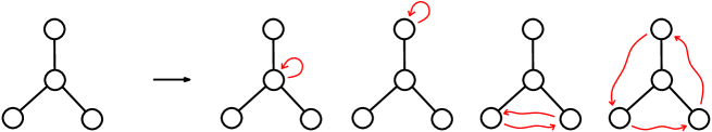
Figure 2. An unlabeled nonplane tree of size $4$ yields 4 unlabeled cycle-pointed trees.

Theorem 5 (unbiased pointing).

Let $\mathcal{A}$ be a species. Then, for $n\geq 0$, each unlabeled structure of $\widetilde{\mathcal{A}}_{n}$ gives rise to exactly $n$ unlabeled structures in $\widetilde{\mathcal{A}^{\circ}_{n}}$; that is, for each $A\in\mathcal{A}[n]$ there are exactly $n$ non-isomorphic structures $(A,c)$ in $\mathcal{A}^{\circ}[n]$. Hence, the ordinary generating series of $\mathcal{A}^{\circ}$ satisfies

$$\widetilde{\mathcal{A}^{\circ}}(x)=x\frac{\mathrm{d}}{\mathrm{d}x}\widetilde{\mathcal{A}}(x).$$ (20)

Proof.

Given $\tilde{A}\in\widetilde{\mathcal{A}}_{n}$, let $S$ be the set of unlabeled pointed structures of $\widetilde{\mathcal{A}^{\circ}}$ whose underlying unpointed structure is $\tilde{A}$. The proof of the lemma reduces to proving that $S$ has cardinality $n$. Let $\mathrm{Sym}(\tilde{A})$ be the set of symmetries for the structure $\tilde{A}$, and let $\mathrm{RSym}(S)$ be the set of rooted c-symmetries for structures from $S$. Lemma 1 shows that $\tilde{A}$ has $n!$ symmetries and Lemma 4 shows that each structure of $\widetilde{\mathcal{A}^{\circ}_{n}}$ has $n!$ rooted c-symmetries. Hence $|\mathrm{Sym}(\tilde{A})|=n!$ and $|\mathrm{RSym}(S)|=|S|n!$. In addition, we have seen that a symmetry $(A,\sigma)$ of size $n$ on $\mathcal{A}$ has $n$ rooted c-symmetries on $\mathcal{A}^{\circ}$. Hence, $|\mathrm{RSym}(S)|=n|\mathrm{Sym}(\tilde{A})|$. Thus, we obtain $|S|n!=nn!$, and therefore $|S|=n$. ∎

Remark 3.1.

Theorem 5 is equivalent to a result known as Parker’s lemma [7, Section 2.8]. For a subgroup $G$ of the symmetric group $\mathfrak{S}_{n}$, say that a cycle $c$ in $g\in G$ is equivalent to a cycle $c^{\prime}$ in $g^{\prime}\in G$ if there exists $h\in G$ that maps the elements of $c$ to the elements of $c^{\prime}$ and preserves the cyclic order, i.e., for each element $x\in c$, the successor of $x$ in $c$ is mapped by $h$ to the successor of $h(x)$ in $c^{\prime}$. Let $a_{k}$ be the number of inequivalent cycles of length $k$. Then Parker’s lemma states that $\sum_{k=1}^{n}a_{k}=n$.

If this lemma is applied to the automorphism group of a fixed structure $A$ of size $n$, then $a_{k}$ is the number of unlabeled cycle-pointed structures arising from $A$ and such that the marked cycle has length $k$. So Parker’s lemma states that there are $n$ unlabeled cycle-pointed structures arising from $A$, i.e., it implies Theorem 5 (conversely, each permutation group is the automorphism group of a structure, so Parker’s lemma can be deduced from Theorem 5).

Remark 3.2.

The classical pointing operator, which selects a single atom in a structure, yields an equation similar to (20) for exponential generating series, which is useful for labeled enumeration. Given a species $\mathcal{A}$, let $\mathcal{A}^{\bullet}$ be the species of structures from $\mathcal{A}$ where an atom is distinguished. Then

$$\mathcal{A}^{\bullet}(x)=x\frac{\mathrm{d}}{\mathrm{d}x}\mathcal{A}(x).$$ (21)

An important contribution of this article is to define a pointing operator $\mathcal{A}\mapsto\mathcal{A}^{\circ}$ that yields the same equation, Equation (20), in the unlabeled case.

3.3. Basic Cycle-pointed Species and Constructions

Basic cycle-pointed species: $\mathcal{A}^{\circ}$, $\mathcal{A}^{{\circledast}}$,${}^{\phantom{1^{\phantom{1^{\phantom{1}}}}}}$
where $\mathcal{A}\in\{{\bf 0},{\bf 1},X,\textsc{Seq}^{[k]},\textsc{Set}^{[k]},\textsc{Cyc}^{[k]},\textsc{Seq},\textsc{Set},\textsc{Cyc}\}$
Pointed cycle-index sum:
$\displaystyle\bar{Z}_{\mathcal{A}^{\circ}}=\sum_{\ell\geq 1}\ell\ t_{\ell}\frac{\partial}{\partial s_{\ell}}Z_{\mathcal{A}}$
$\displaystyle\bar{Z}_{\mathcal{A}^{{\circledast}}}=\sum_{\ell\geq 2}\ell\ t_{\ell}\frac{\partial}{\partial s_{\ell}}Z_{\mathcal{A}}$
Construction	Notation	Pointed cycle index sum
Pointed union	$\mathcal{R}=\mathcal{P}+\mathcal{Q}$	$\bar{Z}_{\mathcal{R}}=\bar{Z}_{\mathcal{P}}+\bar{Z}_{\mathcal{Q}}^{\phantom{1}}$
Pointed product	$\mathcal{R}=\mathcal{P}\star\mathcal{B}$	$\bar{Z}_{\mathcal{R}}=\bar{Z}_{\mathcal{P}}\boldsymbol{\cdot}Z_{\mathcal{B}}$
Pointed substitution	$\mathcal{R}=\mathcal{P}\circledcirc\mathcal{B}$	$\bar{Z}_{\mathcal{R}}=\bar{Z}_{\mathcal{P}}\circledcirc Z_{\mathcal{B}}$

Figure 3. The rules to calculate the pointed cycle index sums of basic cycle-pointed species and of cycle-pointed species composed by $+$, $\star$, and $\circledcirc$.

3.3.1. Basic cycle-pointed species

Species of the form $\mathcal{A}^{\circ}$ or $\mathcal{A}^{{\circledast}}$ where $\mathcal{A}$ is a basic species as introduced in Subsection 2.4 will be called basic cycle-pointed species. The derivation rule in Equation (19) allows us to compute the pointed cycle index sum of basic cycle-pointed species, as indicated in Figure 3 (upper part).

3.3.2. Pointed constructions

It is clear that the disjoint union of two cycle-pointed species as defined in Section 2.4.2 is again a cycle-pointed species. We now adapt the constructions of product and substitution to obtain a pointed product and a pointed substitution operation that produce cycle-pointed species.

Pointed product. Let $\mathcal{A},\mathcal{B}$ be species, and let $\mathcal{P}\subseteq\mathcal{A}^{\circ}$ be a cycle-pointed species. Then the pointed product $\mathcal{P}\star\mathcal{B}$ of $\mathcal{P}$ and $\mathcal{B}$ is the subspecies of $(\mathcal{A}\boldsymbol{\cdot}\mathcal{B})^{\circ}$ of all those structures $((A,B),c)$ in $(\mathcal{A}\boldsymbol{\cdot}\mathcal{B})^{\circ}$ where the pointed cycle $c$ is from $A$, and $(A,c)\in\mathcal{P}$.

Pointed substitution. Let $E=((\pi,A,(B_{p})_{p\in\pi}),c)$ be a structure in $(\mathcal{A}\circ\mathcal{B})^{\circ}$. The study of automorphisms of structures in $\mathcal{A}\circ\mathcal{B}$ performed in Section 2.6.2 shows that

• $c$ is the cycle composed from cycles $c_{1},\ldots,c_{k}$ on different components $B_{p_{1}},\ldots,B_{p_{k}}$;

• the structure $(A,c^{\prime}=(p_{1},...,p_{k}))$ is cycle-pointed.

We call $(A,c^{\prime})\in\mathcal{A}^{\circ}$ the core-structure of $E$.

We can now define a substitution construction for cycle-pointed species. Let $\mathcal{P}\subseteq\mathcal{A}^{\circ}$ and let $\mathcal{B}$ be a species such that $\mathcal{B}[\emptyset]=\emptyset$. Then $\mathcal{P}\circledcirc\mathcal{B}$ is defined as the subspecies of structures from $(\mathcal{A}\circ\mathcal{B})^{\circ}$ whose core-structure is in $\mathcal{P}$.

Figure 4. A cycle-pointed graph obtained from a substitution.

As in the previous section, we make the convention that in expressions involving several of the symbols $+,\boldsymbol{\cdot},\star,\circ,\circledcirc$, the symbols $\circ,\circledcirc$ bind stronger than the symbols $\boldsymbol{\cdot},\star$, and the symbols $\boldsymbol{\cdot},\star$ bind stronger than the symbol $+$.

In a similar way to the labeled framework [2], our pointing operator behaves well with the three constructions $+$, $\boldsymbol{\cdot}$, and $\circ$:

Proposition 6.

The cycle-pointing operator obeys the following rules:

$$\left(\mathcal{A}+\mathcal{B}\right)^{\circ} = \mathcal{A}^{\circ}+\mathcal{B}^{\circ},$$ (22)

$$\left(\mathcal{A}\boldsymbol{\cdot}\mathcal{B}\right)^{\circ} = \mathcal{A}^{\circ}\star\mathcal{B}\ +\ \mathcal{B}^{\circ}\star\mathcal{A},$$ (23)

$$\left(\mathcal{A}\circ\mathcal{B}\right)^{\circ} = \mathcal{A}^{\circ}\circledcirc\mathcal{B}\;.$$ (24)

Proof.

It is easy to see that $(\mathcal{A}+\mathcal{B})^{\circ}$ is isomorphic to $\mathcal{A}^{\circ}+\mathcal{B}^{\circ}$. For the product, note that the pointed cycle $c$ of a structures from $(\mathcal{A}\boldsymbol{\cdot}\mathcal{B})^{\circ}$ has to be entirely on $A$ or entirely on $B$. The species that contains all structures $((A,B),c)$ where $c$ is on $A$ is isomorphic to $\mathcal{A}^{\circ}\star\mathcal{B}$, and the species that contains all structures $((A,B),c)$ where $c$ is on $B$ is isomorphic to $\mathcal{B}^{\circ}\star\mathcal{A}$. Hence, $(\mathcal{A}\boldsymbol{\cdot}\mathcal{B})^{\circ}=\mathcal{A}^{\circ}\star\mathcal{B}+\mathcal{B}^{\circ}\star\mathcal{A}$. For the expression for the substitution operation, we in fact have not only isomorphism, but even equality of species. This is clear from the fact that all core-structures of structures from $(\mathcal{A}\circ\mathcal{B})^{\circ}$ are from $\mathcal{A}^{\circ}$. ∎

As in the unpointed case, there are explicit rules to compute the pointed cycle index sums for each basic species and for each construction. To this end we need the following notion of composition for power series.

Definition 3.3.

Let $f$ and $g$ be two power series of the form $\bar{f}:=f(x_{1},y_{1};x_{2},y_{2};\ldots)$ and $g:=g(x_{1},x_{2},\ldots)$ such that $g(0,0,\ldots)=0$. Then the pointed plethystic composition of $f$ with $g$ is the power series

$$\bar{f}\circledcirc g:=f(g_{1},\bar{h}_{1};g_{2},\bar{h}_{2};\ldots),$$ (25)

with $g_{k}=g(x_{k},x_{2k},x_{3k},\ldots)$ and $\bar{h}_{k}=\bar{h}(x_{k},y_{k};x_{2k},y_{2k};\ldots)$ for $\bar{h}:=\sum_{\ell\geq 1}\ell t_{\ell}\frac{\partial}{\partial s_{\ell}}g$.

The following proposition is the counterpart of Proposition 2 for cycle-pointed species.

Proposition 7 (computation rules for pointed cycle index sums).

For each basic species $\mathcal{A}$, the pointed cycle index sum of the pointed species $\mathcal{A}^{\circ}$ and $\mathcal{A}^{{\circledast}}$ is given by the explicit expression given in Figure 3 (upper part) in terms of the cycle index sum of $\mathcal{A}$. For each of the fundamental pointed constructions $+$, $\star$, and $\circledcirc$ there is an explicit rule, given in Figure 3 (lower part), to compute the pointed cycle index sum of the resulting species.

Proof.

The statement is clear for the cycle-pointed atomic species and the pointed union. Let $\mathcal{A},\mathcal{B}$ be species, and let $\mathcal{P}\subseteq\mathcal{A}^{\circ}$ be a cycle-pointed species. For the cycle-pointed product $\mathcal{Q}=\mathcal{P}\star\mathcal{B}$ notice that, similarly as for a partitional product for species, a rooted c-symmetry on $\mathcal{Q}$ decomposes into a rooted c-symmetry on $\mathcal{P}$ and a symmetry on $\mathcal{B}$, since the automorphism has to act separately on the two component structures. Therefore, $\mathrm{RSym}(\mathcal{Q})$ can be considered as a partitional product of $\mathrm{RSym}(\mathcal{P})$ and $\mathrm{Sym}(\mathcal{B})$, which yields $\bar{Z}_{\mathcal{Q}}=\bar{Z}_{\mathcal{P}}\boldsymbol{\cdot}Z_{\mathcal{B}}$.

For the substitution construction, the proof is similar. Let $\mathcal{P}\subseteq\mathcal{A}^{\circ}$ be a cycle-pointed species and let $\mathcal{B}$ be a species such that $\mathcal{B}[\emptyset]=\emptyset$. Let $\mathcal{Q}=\mathcal{P}\circledcirc\mathcal{B}\subseteq(\mathcal{A}\circ\mathcal{B})^{\circ}$. Consider a rooted c-symmetry $(Q,\sigma,v)$. As we have seen in Section 2.6, the core structure $A$ is endowed with an induced automorphism $\sigma^{\prime}$. In addition, the automorphism is naturally rooted at the atom $v^{\prime}\in A$ where the $\mathcal{B}^{\circ}$-component that contains the root $v$ is substituted. We denote the cycle of $\sigma^{\prime}$ that contains $v^{\prime}$ by $c^{\prime}$. Now we have that $(A,c^{\prime})$ is cycle-pointed and the automorphism $\sigma^{\prime}$ rooted at $v^{\prime}$ is a rooted c-symmetry on $P=(A,c^{\prime})$. In addition, the components substituted at each atom of a cycle $c=(u_{1},\ldots,u_{k})$ of $\sigma^{\prime}$ are isomorphic copies of a same symmetry on $\mathcal{B}$. The components that are substituted at the atoms of the marked cycle $c^{\prime}$ are naturally rooted at the isomorphic representant of $v$. Finally, this decomposition is reversable: one can go back to the original composed symmetry using the composition of cycle operation.

To express these observations in an equation, we define the type of the rooted c-symmetry $(P,\rho,v)$ with $P=(A,c^{\prime})$ to be the sequence $(\ell;n_{1},n_{2},\dots,n_{k})$ where $\ell$ is the length of $c^{\prime}$, and $n_{i}$ is the number of unmarked cycles of length $i$ in $\rho$. Note that the size of $P$ is $\ell+\sum_{i}in_{i}$. The number $a(t)$ of rooted c-symmetries of type $t=(\ell;n_{1},n_{2},\dots,n_{n})$ on $\mathcal{P}$ is $n![t^{\ell}s_{1}^{n_{1}}\cdots s_{n}^{n_{n}}]\bar{Z}_{\mathcal{P}}$. The core type of a rooted c-symmetry on $\mathcal{P}\circledcirc\mathcal{B}$ is defined as the type of the rooted c-symmetry induced on the core structure.

Let $\bar{Z}_{\mathcal{R}}^{(t)}$ be the pointed cycle index sum of $\mathcal{P}$ restricted to the rooted c-symmetries with core-type $t=(\ell;n_{1},n_{2},\dots,n_{n})$. From the above discussion, we have

$$\bar{Z}_{\mathcal{R}}^{(t)}=\frac{a(t)}{n!}q_{\ell}b_{1}^{n_{1}}b_{2}^{n_{2}}\ldots b_{n}^{n_{n}},\ \mathrm{where}\ b_{i}:=Z_{\mathcal{B}}(s_{1},s_{2},\ldots),\ q_{\ell}:=\bar{Z}_{\mathcal{B}^{\circ}}(s_{\ell},t_{\ell};s_{2\ell},t_{2\ell};\ldots).$$ (26)

Summing over all possible types of rooted $c$-symmetries $t$, we obtain
1      $\displaystyle\bar{Z}_{\mathcal{R}}=\bar{Z}_{\mathcal{P}}(b_{1},q_{1};b_{2},q_{2};\ldots),\ \mathrm{where}\ b_{i}:=Z_{\mathcal{B}}(s_{1},s_{2},\ldots),\ q_{\ell}:=\bar{Z}_{\mathcal{B}^{\circ}}(s_{\ell},t_{\ell};s_{2\ell},t_{2\ell};\ldots).$ ∎

In the following we introduce recursive specifications that involve pointed constructions. Cycle-pointed specifications are like standard recursive specifications (Definition 2.5), but with two sorts of variables (where one is reserved for cycle-pointed species) and where we are allowed to use additionally the pointed constructions.

Definition 3.4.

A recursive cycle-pointed specification with variables $x_{1},\dots,x_{m},y_{1},\dots,y_{m^{\prime}}$ over the species $\mathcal{A}_{1},\dots,\mathcal{A}_{\ell}$ and over cycle-pointed species $\mathcal{B}_{1},\dots,\mathcal{B}_{k}$ is a system $\Psi$ of equations $x_{1}=e_{1},\dots,x_{m}=e_{m},y_{1}=f_{1},\dots,y_{m^{\prime}}=f_{m^{\prime}}$ where each $e_{i}$ is

• of the form $a+b$ or $a\boldsymbol{\cdot}b$ with $a,b\in\{x_{1},\ldots,x_{m},\mathcal{A}_{1},\dots,\mathcal{A}_{\ell}\}$, or

• of the form $a\circ b$ with $a\in\{\mathcal{A}_{1},\dots,\mathcal{A}_{\ell}\}$ and $b\in\{x_{1},\dots,x_{m},\mathcal{A}_{1},\dots,\mathcal{A}_{\ell}\}$,

and each $f_{i}$ is

• of the form $a+b$ with $a,b\in\{y_{1},\ldots,y_{m^{\prime}},\mathcal{B}_{1},\dots,\mathcal{B}_{k}\}$, or

• of the form $a\star b$ with $a\in\{y_{1},\ldots,y_{m^{\prime}},\mathcal{B}_{1},\dots,\mathcal{B}_{k}\}$ and $b\in\{x_{1},\ldots,x_{m},\mathcal{A}_{1},\dots,\mathcal{A}_{\ell}\}$, or

• of the form $a\circledcirc b$ with $a\in\{\mathcal{B}_{1},\dots,\mathcal{B}_{k}\}$ and $b\in\{x_{1},\dots,x_{m},\mathcal{A}_{1},\dots,\mathcal{A}_{\ell}\}$.

To define the species $\mathcal{X}_{1},\dots,\mathcal{X}_{m},\mathcal{Y}_{1},\dots,\mathcal{Y}_{m^{\prime}}$ that are given by a recursive cycle-pointed specification $\Psi$ with variables $x_{1},\dots,x_{m},y_{1},\dots,y_{m^{\prime}}$ over the species $\mathcal{A}_{1},\dots,\mathcal{A}_{\ell},\mathcal{B}_{1},\dots,\mathcal{B}_{k}$ where $\mathcal{B}_{1},\dots,\mathcal{B}_{k}$ are pointed, we again (as in Section 2.5) consider sequences of species $\mathcal{X}_{j}^{(i)}$ and $\mathcal{Y}_{j}^{(i)}$ for $i\geq 1$. For $i=1$, we define $\mathcal{X}_{j}^{(i)}=\bf 0$ for all $1\leq j\leq m$, and $\mathcal{Y}_{j}^{(i)}=\bf 0^{\circ}$ for all $1\leq j\leq{m^{\prime}}$. For $i>1$ the species $\mathcal{X}^{(i)}_{j}$ and $\mathcal{Y}^{(i)}_{j}$ are obtained by evaluating the corresponding expressions for $x_{j}$ and $y_{j}$, respectively (as in Section 2.5). We say that $\Psi$ is admissible if in expressions of the form $a\circ b$ or $a\circledcirc b$ the species substituted for $b$ never contain structures of size $0$.

Note that also the new pointed constructions are monotone, so in case that for each $n$ the sets $\bigcup_{i\geq 1}\mathcal{X}^{(i)}[n]$ and $\bigcup_{i\geq 1}\mathcal{Y}^{(i)}[n]$ are finite it is straightforward (and analogous to Definition 2.6) to define the species $\mathcal{X}_{1},\dots,\mathcal{X}_{m},\mathcal{Y}_{1},\dots,\mathcal{Y}_{m^{\prime}}$ specified by admissible recursive specifications $\Psi$ over $\mathcal{A}_{1},\dots,\mathcal{A}_{\ell},\mathcal{B}_{1},\dots,\mathcal{B}_{k}$.

Definition 3.5.

Let $\mathfrak{A}$ be a class of species. The class of species that is cycle-pointing decomposable over $\mathfrak{A}$ is the smallest class of species $\mathfrak{B}$ that contains $\mathfrak{A}$, contains all species that can be specified by cycle-pointed recursive specifications over pointed and unpointed species from $\mathfrak{B}$, and contains all species obtained from species of the form $\mathcal{A}^{\circ}$ in $\mathfrak{B}$ by applying the unpointing operation.

Plenty of examples of species that are decomposable over simple basic species can be found in Section 4.

Proposition 8.

If a species $\mathcal{A}$ is decomposable (in the sense of Definition 2.7), then the pointed species $\mathcal{A}^{\circ}$ is cycle-pointing-decomposable.

Proof.

Follows directly from Proposition 6. ∎

Remark 3.3.

The ordinary generating series inherit simple computation rules from the ones for pointed cycle index sums. As expected, for the sum and product constructions, one gets

$$\mathcal{R}=\mathcal{P}+\mathcal{Q} \Rightarrow \widetilde{\mathcal{R}}(x)=\widetilde{\mathcal{P}}(x)+\widetilde{\mathcal{Q}}(x),$$ (27)

$$\mathcal{Q}=\mathcal{P}\star\mathcal{B} \Rightarrow \widetilde{\mathcal{Q}}(x)=\widetilde{\mathcal{P}}(x)\cdot\widetilde{\mathcal{B}}(x).$$ (28)

For the substitution construction, the computation rule is:

$$\hskip 28.45274pt\mathcal{Q}=\mathcal{P}\circledcirc\mathcal{B} \Rightarrow \widetilde{\mathcal{Q}}(x)=\bar{Z}_{\mathcal{P}}(\widetilde{\mathcal{B}}(x),\widetilde{\mathcal{B}^{\circ}}(x);\widetilde{\mathcal{B}}(x^{2}),\widetilde{\mathcal{B}^{\circ}}(x^{2});\ldots),$$ (29)

where $\widetilde{\mathcal{B}^{\circ}}(x)=x\frac{\mathrm{d}}{\mathrm{d}x}\widetilde{\mathcal{B}}(x)$. Hence, to compute the ordinary generating series of a decomposable cycle-pointed species, the only place where the cycle index sum or pointed cycle index sum is needed (as a refinement of ordinary generating series) is for the species that is the first argument of a substitution or pointed substitution construction.

Remark 3.4.

As an exercise, the reader can check just by standard algebraic manipulations that the computation rules for cycle-index sums are consistent with Proposition 6. For instance, proving $\bar{Z}_{(\mathcal{A}\circ\mathcal{B})^{\circ}}=\bar{Z}_{\mathcal{A}^{\circ}\circledcirc\mathcal{B}}$ is equivalent (by the computation rules) to proving the equality $\bar{Z}_{(\mathcal{A}\circ\mathcal{B})^{\circ}}=\bar{Z}_{\mathcal{A}^{\circ}}\circledcirc Z_{\mathcal{B}}$, which reduces to checking the following identity on power series:

$$\Delta(f\circ g)=(\Delta f)\circledcirc g\;,$$ (30)

where $\Delta$ is the operator that associates to a power series $f(x_{1},x_{2},x_{3},\ldots)$ the power series

$$\Delta f(x_{1},y_{1};x_{2},y_{2};\ldots):=\sum_{\ell\geq 1}\ell\ y_{\ell}\frac{\partial}{\partial x_{\ell}}f(x_{1},x_{2},x_{3},\ldots).$$

Similarly, to prove $\bar{Z}_{(\mathcal{A}+\mathcal{B})^{\circ}}=\bar{Z}_{\mathcal{A}^{\circ}+\mathcal{B}^{\circ}}$ and $\bar{Z}_{(\mathcal{A}\boldsymbol{\cdot}\mathcal{B})^{\circ}}=\bar{Z}_{\mathcal{A}^{\circ}\star\mathcal{B}+\mathcal{B}^{\circ}\star\mathcal{A}}$, one has to check the identities $\Delta(f+g)=\Delta f+\Delta g$, and $\Delta(f\cdot g)=\Delta f\cdot g+f\cdot\Delta g$, respectively.

4. Application to Enumeration

In this section we demonstrate that cycle-pointing provides a new way of counting many classes of combinatorial structures in the unlabeled setting. Typically, species satisfying a “tree-like” decomposition are amenable to our method. This includes of course species of trees, but also species of graphs (provided that the species is closed under taking 2-connected components, and that the sub-species of 2-connected graphs is tractable), and species of planar maps.

The general scheme to enumerate unlabeled structures of a species $\mathcal{A}$, i.e., to obtain the coefficients $|\widetilde{\mathcal{A}_{n}}|$, is as follows. First, we observe that the task is equivalent to the task to enumerate unlabeled cycle-pointed structures from $\mathcal{A}^{\circ}$, because $|\widetilde{\mathcal{A}^{\circ}_{n}}|=n|\widetilde{\mathcal{A}_{n}}|$. Enumeration for $\mathcal{A}^{\circ}$ turns out to be easier since the marked cycle usually provides a starting point for a recursive decomposition.

For a cycle-pointed species of trees (and more generally for species satisfying tree-like decompositions), the first step of the decomposition scheme is to distinguish whether the marked cycle has length $1$ or greater than $1$. The general equation is

$$\mathcal{A}^{\circ}=X^{\circ}\star\mathcal{A}^{\prime}+\mathcal{A}^{{\circledast}},$$ (31)

where $\mathcal{A}^{\prime}$ is the derived species of $\mathcal{A}$, consisting of structures from $\mathcal{A}$ where one atom is marked with a special label, say $*$, as defined in [2]. Then each of the two species $\mathcal{A}^{\prime}$ and $\mathcal{A}^{{\circledast}}$ has to be decomposed. For derived structures (the species $\mathcal{A}^{\prime}$) we follow the classical root decomposition. For symmetric cycle-pointed structures (the species $\mathcal{A}^{{\circledast}}$) our decomposition strategy is different, and leads us to introduce the notion of center of symmetry.

4.1. Trees

We first illustrate our decomposition method for trees, which are defined as connected acyclic graphs (i.e., unless mentioned otherwise, trees are unrooted), and we start with the formal definition of the center of symmetry. Let $T$ be a symmetric cycle-pointed tree. A path of $T$ connecting two consecutive atoms of the marked cycle is called a connecting path (thus the number of connecting paths is the size of the marked cycle).

Claim 9 (center of symmetry).

Given a symmetric cycle-pointed tree $T$, all connecting paths of $T$ share the same middle $v_{c}$, called the central point for the marked cycle of $T$. The central point $v_{c}$ is the middle of an edge $e$ if these paths have odd length, and is a vertex $v$ if these paths have even length. In the first (second) case, the edge $e$ (the vertex $v$, resp.) is called the center of symmetry of $T$.

Proof.

We prove here that all connecting paths share the same middle. Let $U$ be the subgraph of $T$ formed by the union of all connecting paths. Observe that $U$ is connected, so $U$ is a subtree of $T$. In addition, $U$ is globally fixed by any c-automorphism of $T$ (indeed, the property of being on a connecting path is invariant under the action of a c-automorphism), and it contains the atoms of the marked cycle of $T$. Hence $U$ is the underlying structure of a cycle-pointed tree $(U,c)$. Consider the classical center of $U$, obtained by pruning the leaves (at each step, all leaves are simultaneously deleted) until the resulting tree is reduced to an edge or a vertex [2]. The central point $v_{c}$ of $U$ is defined as follows: if the center of $U$ is a vertex $v$, then $v_{c}:=v$, if the center of $U$ is an edge $e$, then $v_{c}$ is the middle of $e$. Let $\sigma$ be a c-automorphism of $(U,c)$ and let $\langle\sigma\rangle$ be the group of automorphisms generated by $\sigma$. It is well known that the central point is fixed by any automorphism on the tree, hence $v_{c}$ is equidistant from all atoms of the marked cycle, as the group $\langle\sigma\rangle$ acts transitively on the vertices of the marked cycle. In addition, $v_{c}$ is on at least one connecting path of $T$ (because $U$ is the union of these connecting paths). Hence, $v_{c}$ has to be on all connecting paths, as the group $\langle\sigma\rangle$ acts transitively on the connecting paths. Thus, $v_{c}$ has to be the middle of all connecting paths simultaneously. ∎

Remark 4.1.

Notice that the center of symmetry might not coincide with the classical center of the tree, as shown in Figure 5. However, in the case of plane trees, the two notions of center coincide.

Figure 5. Decomposition of a nonplane tree at its center of symmetry (in case the center of symmetry is a vertex).

4.1.1. Nonplane trees

Let $\mathcal{F}$ be the species of free trees, i.e., unrooted nonplane trees (equivalently, acyclic connected graphs), where the vertices are taken as atoms. Let $\mathcal{F}\ \!^{\prime}$ be the derived species of $\mathcal{F}$ (also the species of derived nonplane trees). Rooted nonplane trees can be decomposed at the root. Since the root does not count as an atom and since the children of the root node are unordered, we classically have

$$\mathcal{F}\ \!^{\prime}=\textsc{Set}\circ(X\boldsymbol{\cdot}\mathcal{F}\ \!^{\prime}).$$ (32)

In contrast, the decomposition of symmetric cycle-pointed trees does not start at atoms of the marked cycle, but at the center of symmetry, which is either an edge or a vertex (see Figure 5 for an illustration of the decomposition). In order to write down the decomposition, we introduce the species $\mathcal{L}$ consisting of a single one-edge graph. Note that $\mathcal{L}\simeq\textsc{Set}^{[2]}$, and that $\mathcal{L}^{{\circledast}}$ consists of the link graph carrying a marked cycle of length 2 that exchanges the two extremities of the edge.

Claim 10.

The species $\mathcal{F}^{{\circledast}}$ of symmetric cycle-pointed free trees satisfies

$$\mathcal{F}^{{\circledast}}=\mathcal{L}^{{\circledast}}\circledcirc\mathcal{R}+X\boldsymbol{\cdot}\textsc{Set}^{{\circledast}}\circledcirc\mathcal{R},$$ (33)

where $\mathcal{R}:=X\boldsymbol{\cdot}\mathcal{F}$ is the species of all pointed trees.

Proof.

Consider a tree produced from the species $\mathcal{L}^{{\circledast}}\circledcirc\mathcal{R}+X\boldsymbol{\cdot}\textsc{Set}^{{\circledast}}\circledcirc\mathcal{R}$ (for an example of a tree produced from $X\boldsymbol{\cdot}\textsc{Set}^{{\circledast}}\circledcirc\mathcal{R}$, see the transition between the right and the left drawing in Figure 5). Clearly, such a tree is free and cycle-pointed and it is symmetric because the marked cycle of the core-structure – an edge $e$ in the first case, a cycle-pointed set attached to a vertex $v$ in the second case – already has length greater than 1. Hence $\mathcal{F}^{{\circledast}}\supseteq\mathcal{L}^{{\circledast}}\circledcirc\mathcal{R}+X\boldsymbol{\cdot}\textsc{Set}^{{\circledast}}\circledcirc\mathcal{R}^{\circ}$. Notice also that in the first (second) case, $e$ ($v$, respectively) is the center of symmetry of the resulting tree. Indeed each connecting path connects vertices on two different subtrees attached at the center of symmetry, which, by symmetry, stands in the middle of such a path.

Conversely, for each symmetric cycle-pointed free tree $T$, we color blue its center of symmetry, which plays the role of a core-structure for $T$. Partition $\mathcal{F}^{{\circledast}}$ as $\mathcal{F}_{\mathrm{v}}^{{\circledast}}+\mathcal{F}_{\mathrm{e}}^{{\circledast}}$, where $\mathcal{F}_{\mathrm{v}}^{{\circledast}}$ ($\mathcal{F}_{\mathrm{e}}^{{\circledast}}$, respectively) gathers the trees in $\mathcal{F}^{{\circledast}}$ whose center of symmetry is a vertex (an edge, respectively). Define also $\mathcal{M}_{\mathrm{v}}$ ($\mathcal{M}_{\mathrm{e}}$) as the species of free trees with a distinguished vertex (edge, resp.) that is colored blue. Clearly $\mathcal{M}_{\mathrm{v}}=X\boldsymbol{\cdot}(\textsc{Set}\circ\mathcal{R})$ and $\mathcal{M}_{\mathrm{e}}=\mathcal{L}\circ\mathcal{R}$. From Proposition 6, we obtain $\mathcal{M}_{\mathrm{v}}^{{\circledast}}=X^{\circ}\star(\textsc{Set}\circ\mathcal{R})+X\boldsymbol{\cdot}\textsc{Set}^{\circ}\circledcirc\mathcal{R}$ and $\mathcal{M}_{\mathrm{e}}^{\circ}=\mathcal{L}^{\circ}\circledcirc\mathcal{R}$. Observe that $\mathcal{F}_{\mathrm{v}}^{{\circledast}}$ ($\mathcal{F}_{\mathrm{e}}^{{\circledast}}$) contains the structures of $\mathcal{M}_{\mathrm{v}}^{{\circledast}}$ (of $\mathcal{M}_{\mathrm{e}}^{{\circledast}}$) where the blue vertex (edge, resp.) is the center of symmetry. It is clear that the structures of $X^{\circ}\star(\textsc{Set}\circ\mathcal{R})$ have their marked cycle of length 1, so they are not in $\mathcal{F}_{\mathrm{v}}^{{\circledast}}$. Concerning the structures of $X\boldsymbol{\cdot}\textsc{Set}^{\circ}_{(1)}\circledcirc\mathcal{R}$, the atoms of the marked cycle are on a same subtree attached at the blue vertex, so that the blue vertex is not the center of symmetry. Hence the structures of $X\boldsymbol{\cdot}\textsc{Set}^{\circ}_{(1)}\circledcirc\mathcal{R}$ are not in $\mathcal{F}_{\mathrm{v}}^{{\circledast}}$. Similarly, the structures of $\mathcal{L}^{\circ}_{(1)}\circledcirc\mathcal{R}$ are not in $\mathcal{F}_{\mathrm{e}}^{{\circledast}}$. Therefore we obtain the second inclusion $\mathcal{F}^{{\circledast}}\subseteq\mathcal{L}^{{\circledast}}\circledcirc\mathcal{R}+X\boldsymbol{\cdot}\textsc{Set}^{{\circledast}}\circledcirc\mathcal{R}$. ∎

Proposition 11 (decomposing and counting free trees).

The species $\mathcal{F}^{\circ}$ of cycle-pointed free trees has the following cycle-pointed recursive specification over the species Set, $\mathcal{L}^{{\circledast}}$, $X$:

$$\left\{\begin{array}[]{rcl}\mathcal{F}^{\circ}&=&X^{\circ}\star\mathcal{F}\ \!^{\prime}+\mathcal{F}^{{\circledast}},\\ \mathcal{F}\ \!^{\prime}&=&\textsc{Set}\circ\mathcal{R},\ \ \mathcal{R}=X\boldsymbol{\cdot}\mathcal{F}\ \!^{\prime},\\ \mathcal{F}^{{\circledast}}&=&\mathcal{L}^{{\circledast}}\circledcirc\mathcal{R}+X\boldsymbol{\cdot}\textsc{Set}^{{\circledast}}\circledcirc\mathcal{R},\\ \mathcal{R}^{\circ}&=&X^{\circ}\star(\textsc{Set}\circ\mathcal{R})+X\boldsymbol{\cdot}\textsc{Set}^{\circ}\circledcirc\mathcal{R},\end{array}\right.$$ (34)

The ordinary generating function $f(x):=\widetilde{\mathcal{F}}(x)$ of free trees satisfies the equations

$$xf^{\prime}(x) = r(x)+x^{2}r^{\prime}(x^{2})+\left(\sum_{\ell\geq 2}x^{\ell}r^{\prime}(x^{\ell})\right)r(x)$$ (35)

$$= xr^{\prime}(x)(1-r(x))+x^{2}r^{\prime}(x^{2}),$$ (36)

where $r(x)$ is specified by $\displaystyle r(x)=x\exp\left(\sum_{i\geq 1}\frac{1}{i}r(x^{i})\right)$.

Proof.

The first three lines of the grammar are Equations (31), (32), and (33), respectively. The fourth line is obtained from the second line (i.e., $\mathcal{R}=X\boldsymbol{\cdot}(\textsc{Set}\circ\mathcal{R})$) using the derivation rules of Proposition 6.

Concerning the OGSs, let $r(x):=\widetilde{\mathcal{R}}(x)$ be the OGS of the species $\mathcal{R}$. Note that $\widetilde{\mathcal{F}^{\circ}}(x)=xf^{\prime}(x)$ and $\widetilde{\mathcal{R}^{\circ}}(x)=xr^{\prime}(x)$ by Theorem 5. By the computation rules for OGSs (Remark 2.1 and Remark 3.3), the second line of the grammar, i.e., $\mathcal{R}=X\boldsymbol{\cdot}(\textsc{Set}\circ\mathcal{R})$, yields $r(x)=x\exp(\sum_{i\geq 1}r(x^{i})/i)$; and the third line of the grammar yields

$$\widetilde{\mathcal{F}^{{\circledast}}}(x)=\overline{Z}_{\mathcal{L}^{{\circledast}}}(r(x),xr^{\prime}(x);r(x^{2}),x^{2}r^{\prime}(x^{2});\ldots)+x\overline{Z}_{\textsc{Set}^{{\circledast}}}(r(x),xr^{\prime}(x);r(x^{2}),x^{2}r^{\prime}(x^{2});\ldots).$$

Applying the derivation rule (19) to $\mathcal{L}=\textsc{Set}^{[2]}$ and Set, we get the expressions $\overline{Z}_{\mathcal{L}^{{\circledast}}}\!=\!t_{2}$ and $\overline{Z}_{\textsc{Set}^{{\circledast}}}\!=\!(\sum_{\ell\geq 2}t_{\ell})\boldsymbol{\cdot}Z_{\textsc{Set}}$. Hence $\widetilde{\mathcal{F}^{{\circledast}}}(x)\!=\!x^{2}r^{\prime}(x^{2})+\big{(}\sum_{\ell\geq 2}x^{\ell}r^{\prime}(x^{\ell})\big{)}\cdot r(x)$. Finally, the first line of the grammar yields $\widetilde{\mathcal{F}^{\circ}}(x)=r(x)+\widetilde{\mathcal{F}^{{\circledast}}}(x)$, which gives Expression (35) of $xf^{\prime}(x)$. Using $xr^{\prime}(x)=r(x)(1+\sum_{\ell\geq 1}x^{\ell}r^{\prime}(x^{\ell}))$, this expression simplifies to Expression (36) of $xf^{\prime}(x)$. ∎

Remark 4.2.

The expression $xf^{\prime}(x)=xr^{\prime}(x)(1-r(x))+x^{2}r^{\prime}(x^{2})$ clearly agrees with Otter’s formula [26]:

$$f(x)=r(x)-\frac{1}{2}(r^{2}(x)-r(x^{2})),$$ (37)

which can be obtained either from Otter’s dissimilarity equation or from the dissymmetry theorem [2]. The new result of our method is to yield an expression for $xf^{\prime}(x)$ – Equation (35) – that has only positive signs, as it reflects a positive decomposition grammar. This is crucial to obtain random generators without rejection in Section 5.

All the arguments we have used for free trees can be adapted to decompose and enumerate species $\mathcal{F}_{\Omega}$ of trees where the degrees of the vertices lie in a finite integer set $\Omega$ that contains $1$. It is helpful to define the auxiliary species $\mathcal{R}_{\Omega}$ that consists of trees from $\mathcal{F}_{\Omega}$ rooted at a leaf that does not count as an atom. By decomposing trees at the root, we note that $\mathcal{R}_{\Omega}$ has the recursive specification

$$\mathcal{R}_{\Omega}=X\boldsymbol{\cdot}\textsc{Set}_{\Omega-1}\circ\mathcal{R}_{\Omega},\ \ \mathrm{with}\ \ \textsc{Set}_{\Omega-1}:=\cup_{k\in\Omega}\textsc{Set}^{[k-1]}\;.$$

The species $\mathcal{R}_{\Omega}$ serves as elementary rooted species to express the pointed species arising from $\mathcal{F}_{\Omega}$.

Proposition 12 (decomposing and counting degree-constrained trees).

For any finite set $\Omega$ of positive integers containing $1$, let $\mathcal{F}_{\Omega}$ be the species of nonplane trees whose vertex degrees are in $\Omega$. Then the species $\mathcal{F}_{\Omega}^{\circ}$ has the following cycle-pointed recursive specification, where $\textsc{Set}_{\Omega}:=\cup_{k\in\Omega}\textsc{Set}^{[k]}$ and $\textsc{Set}_{\Omega-1}:=\cup_{k\in\Omega}\textsc{Set}^{[k-1]}$:

$$\left\{\begin{array}[]{rcl}\mathcal{F}_{\Omega}^{\circ}&=&X^{\circ}\star\mathcal{F}_{\Omega}\ \!^{\prime}+\mathcal{F}_{\Omega}^{{\circledast}},\\ \mathcal{F}_{\Omega}\ \!^{\prime}&=&\textsc{Set}_{\Omega}\circ\mathcal{R}_{\Omega},\ \ \mathcal{R}_{\Omega}=X\boldsymbol{\cdot}\textsc{Set}_{\Omega-1}\circ\mathcal{R}_{\Omega},\\ \mathcal{F}_{\Omega}^{{\circledast}}&=&\mathcal{L}^{{\circledast}}\circledcirc\mathcal{R}_{\Omega}+X\boldsymbol{\cdot}\textsc{Set}_{\Omega}^{{\circledast}}\circledcirc\mathcal{R}_{\Omega},\\ \mathcal{R}_{\Omega}^{\circ}&=&X^{\circ}\star\textsc{Set}_{\Omega}\circ\mathcal{R}_{\Omega}+X\boldsymbol{\cdot}\textsc{Set}_{\Omega}^{\circ}\circledcirc\mathcal{R}_{\Omega}.\end{array}\right.$$ (38)

The ordinary generating function $f_{\Omega}(x):=\widetilde{\mathcal{F}_{\Omega}}(x)$ satisfies the equation

$$xf_{\Omega}^{\prime}(x)=xZ_{\textsc{Set}_{\Omega}}(r_{\Omega}(x),r_{\Omega}(x^{2}),\ldots)+x^{2}r_{\Omega}^{\prime}(x^{2})+x\overline{Z}_{\textsc{Set}_{\Omega}^{{\circledast}}}(r_{\Omega}(x),xr_{\Omega}^{\prime}(x);r_{\Omega}(x^{2}),x^{2}r_{\Omega}^{\prime}(x^{2});\ldots),$$ (39)

where $r_{\Omega}(x)$ is specified by $\displaystyle r_{\Omega}(x)=x\boldsymbol{\cdot}Z_{\textsc{Set}_{\Omega-1}}(r_{\Omega}(x),r_{\Omega}(x^{2}),r_{\Omega}(x^{3}),\ldots)$. The power series $Z_{\textsc{Set}_{\Omega-1}}$, $Z_{\textsc{Set}_{\Omega}}$ and $\overline{Z}_{\textsc{Set}_{\Omega}^{{\circledast}}}$ appearing in the equation are polynomials that can be computed explicitly.

Example 1. Unrooted nonplane binary trees. Trees whose vertex degrees are in $\Omega:=\{1,3\}$ are called unrooted nonplane binary trees (note that rooting such a tree at a leaf, one obtains a rooted nonplane binary tree, i.e., each internal node has two unordered children). In that case, the elementary cycle index sums required in Equation (39) are

$$Z_{\textsc{Set}_{\Omega-1}}=1+\frac{1}{2}s_{1}^{2}+\frac{1}{2}s_{2},\ \ Z_{\textsc{Set}_{\Omega}}=s_{1}+\frac{1}{6}s_{1}^{3}+\frac{1}{2}s_{1}s_{2}+\frac{1}{3}s_{3},\ \ \overline{Z}_{\textsc{Set}_{\Omega}^{{\circledast}}}=t_{2}s_{1}+t_{3}.$$

Let $f(x)$ be the OGS of unrooted nonplane binary trees and $r(x)$ the OGS of rooted nonplane binary trees (rooted at a leaf that does not count as an atom). Firstly, from the expression of $Z_{\textsc{Set}_{\Omega-1}}$ one obtains

$$r(x)=x\boldsymbol{\cdot}(1+\frac{1}{2}r(x)^{2}+\frac{1}{2}r(x^{2})).$$

Then, Equation (39) yields

$$xf^{\prime}(x)=x\boldsymbol{\cdot}(r(x)+\frac{1}{6}r(x)^{3}+\frac{1}{2}r(x)r(x^{2})+\frac{1}{3}r(x^{3}))+x^{2}r^{\prime}(x^{2})+x\boldsymbol{\cdot}(x^{2}r^{\prime}(x^{2})r(x)+x^{3}r^{\prime}(x^{3})),$$

i.e.,

$$f^{\prime}(x)=r(x)+\frac{1}{6}r(x)^{3}+\frac{1}{2}r(x)r(x^{2})+\frac{1}{3}r(x^{3})+xr^{\prime}(x^{2})\boldsymbol{\cdot}(1+xr(x))+x^{3}r^{\prime}(x^{3}).$$

From this equation one can extract the counting coefficients of unrooted nonplane binary trees with respect to the number of vertices (after extracting first the coefficients of $r(x)$):

$$xf^{\prime}(x)=2\cdot\mathbf{1}\cdot x^{2}+4\cdot\mathbf{1}\cdot x^{4}+6\cdot\mathbf{1}\cdot x^{6}+8\cdot\mathbf{1}\cdot x^{8}+10\cdot\mathbf{2}\cdot x^{10}+12\cdot\mathbf{2}\cdot x^{12}+14\cdot\mathbf{4}\cdot x^{14}+16\cdot\mathbf{6}\cdot x^{16}+\ldots$$

Hence the first counting coefficients with respect to the number of internal nodes (starting with $0$ internal nodes) are $1$, $1$, $1$, $1$, $2$, $2$, $4$, $6$. Pushing further one gets $1$, $1$, $1$, $1$, $2$, $2$, $4$, $6$, $11$, $18$, $37$, $66$, $135$, $265$, $552$, $1132$, which coincides with Sequence A000672 in [32] (the number of trivalent trees with $n$ nodes).  $\square$

4.1.2. Plane trees.

A plane tree is a tree endowed with an explicit embedding in the plane. Hence, a plane tree is a tree where the cyclic order around each vertex matters. Let $\mathcal{E}$ be the species of plane trees, where again the atoms are the vertices. As usual the startegy to count plane trees is to decompose $\mathcal{E}^{\circ}$, distinguishing whether the marked cycle has length $1$ or larger than $1$:

$$\mathcal{E}^{\circ}=X^{\circ}\star\mathcal{E}^{\prime}+\mathcal{E}^{{\circledast}}.$$ (40)

The species $\mathcal{E}^{\prime}$ is decomposed with the help of another species of plane trees: denote by $\mathcal{A}$ the species of plane trees rooted at a leaf which does not count as an atom. Decomposing $\mathcal{A}$ at the root, we get

$$\mathcal{A}=X\boldsymbol{\cdot}\textsc{Seq}\circ\mathcal{A}.$$ (41)

Again the species $\mathcal{A}$ serves as elementary rooted species to express species of pointed plane trees:

Proposition 13 (decomposing and counting plane trees).

The species $\mathcal{E}^{\circ}$ of cycle-pointed plane trees has the following cycle-pointed recursive specification.

$$\left\{\begin{array}[]{rcl}\mathcal{E}^{\circ}&=&X^{\circ}\star\mathcal{E}\ \!^{\prime}+\mathcal{E}^{{\circledast}},\\ \mathcal{E}\ \!^{\prime}&=&\textsc{Cyc}\circ\mathcal{A},\ \ \mathcal{A}=X\boldsymbol{\cdot}\textsc{Seq}\circ\mathcal{A},\\ \mathcal{E}^{{\circledast}}&=&\mathcal{L}^{{\circledast}}\circledcirc\mathcal{A}+X\boldsymbol{\cdot}\textsc{Cyc}^{{\circledast}}\circledcirc\mathcal{A},\\ \mathcal{A}^{\circ}&=&X^{\circ}\star\textsc{Seq}\circ\mathcal{A}+X\boldsymbol{\cdot}\textsc{Seq}^{\circ}\circledcirc\mathcal{A},\end{array}\right.$$ (42)

The ordinary generating function $\widetilde{\mathcal{E}}(x)$ of plane trees satisfies the equation:

$$e^{\prime}(x) = 1+\sum_{\ell\geq 1}\frac{\phi(\ell)}{\ell}\log\frac{1}{1-a(x^{\ell})}+xa^{\prime}(x^{2})+\sum_{\ell\geq 2}\phi(\ell)\frac{x^{\ell}a^{\prime}(x^{\ell})}{1-a(x^{\ell})},$$ (43)

where $a(x)$ is the series of Catalan numbers: $\displaystyle a(x)=\frac{1}{2}\big{(}\ \!1-\sqrt{1-4x}\ \!\big{)}=\sum_{n\geq 0}\frac{1}{n+1}\binom{2n}{n}x^{n+1}$.

By coefficient extraction, one gets the following formula for the number $e_{n}$ of plane trees with $n+1$ vertices (entry A002995 in [32]):

$$e_{n}=\frac{1}{n+1}\Big{[}\frac{1}{2n}\binom{2n}{n}+\frac{n+1}{2n}\sum_{k|n,k\neq n}\phi(n/k)\binom{2k}{k}+\mathbf{1}_{\left\{\begin{subarray}{c}n\ \mathrm{odd}\\ n=2n^{\prime}\!+\!1\end{subarray}\right\}}\cdot\binom{2n^{\prime}}{n^{\prime}}\Big{]}.$$ (44)

Proof.

The grammar is obtained by arguments similar to those used to derive the grammar (34) for free trees. The only difference is that the cyclic order of the neighbors around each vertex matters, so a Set construction in the grammar for free trees typically has to be replaced by a Cyc construction in the grammar for plane trees. ∎

All the arguments apply similarly for species of plane trees where the degrees of vertices are constrained. As a counterpart to Proposition 11, we obtain:

Proposition 14 (decomposing and counting degree-constrained plane trees).

For any finite set $\Omega$ of positive integers containing $1$, let $\mathcal{E}_{\Omega}$ be the species of free trees where the degrees of vertices are constrained to lie in $\Omega$. Then the cycle-pointed species $\mathcal{E}_{\Omega}^{\circ}$ is decomposable, it satisfies the following decomposition grammar, where $\textsc{Cyc}_{\Omega}:=\cup_{k\in\Omega}\textsc{Cyc}^{[k]}$ and $\textsc{Seq}_{\Omega-1}:=\cup_{k\in\Omega}\textsc{Seq}^{[k-1]}$:

$$\left\{\begin{array}[]{rcl}\mathcal{E}_{\Omega}^{\circ}&=&X^{\circ}\star\mathcal{E}_{\Omega}\ \!^{\prime}+\mathcal{E}_{\Omega}^{{\circledast}},\\ \mathcal{E}_{\Omega}\ \!^{\prime}&=&\textsc{Cyc}_{\Omega}\circ\mathcal{A}_{\Omega},\ \ \mathcal{A}_{\Omega}=X\boldsymbol{\cdot}\textsc{Seq}_{\Omega-1}\circ\mathcal{A}_{\Omega},\\ \mathcal{E}_{\Omega}^{{\circledast}}&=&\mathcal{L}^{{\circledast}}\circledcirc\mathcal{A}_{\Omega}+X\boldsymbol{\cdot}\textsc{Cyc}_{\Omega}^{{\circledast}}\circledcirc\mathcal{A}_{\Omega},\\ \mathcal{A}_{\Omega}^{\circ}&=&X^{\circ}\star\textsc{Seq}_{\Omega-1}\circ\mathcal{A}_{\Omega}+X\boldsymbol{\cdot}\textsc{Seq}_{\Omega-1}^{\circ}\circledcirc\mathcal{A}_{\Omega}.\end{array}\right.$$ (45)

The ordinary generating function $e_{\Omega}(x):=\widetilde{\mathcal{E}_{\Omega}}(x)$ satisfies the equation:

$$e_{\Omega}\ \!^{\prime}(x)=\sum_{\begin{subarray}{c}k\in\Omega\\ r|k\end{subarray}}\frac{\phi(r)}{k}a_{\Omega}(x^{r})^{k/r}+xa_{\Omega}\ \!^{\prime}(x^{2})+\sum_{\begin{subarray}{c}k\in\Omega\\ r|k,r>1\end{subarray}}\phi(r)x^{r}a_{\Omega}\ \!^{\prime}(x^{r})a_{\Omega}(x^{r})^{k/r-1},$$ (46)

where $a_{\Omega}(x)$ is specified by $\displaystyle a_{\Omega}(x)=x\sum_{k\in\Omega}a_{\Omega}(x)^{k-1}$.

Example 2. $d$-regular plane trees. For $d\geq 3$, a $d$-regular plane tree is a plane tree such that each internal node has degree $d$, which corresponds to the case $\Omega=\{1,d\}$ in Proposition 14. It is easily shown that such a tree with $n$ internal nodes has $m=n(d-2)+2$ leaves. Let $\mathcal{E}_{[d]}$ be the species of $d$-regular plane trees, where the atoms are the leaves (it proves here more convenient to take leaves as atoms and to write the counting coefficients according to the number of internal vertices). Let $\mathcal{A}_{[d]}:=\mathcal{E}_{[d]}\ \!\!\!^{\prime}$ be the corresponding derived species, which satisfies $\mathcal{A}_{[d]}=X+(\mathcal{A}_{[d]})^{d-1}$. The decomposition for the cycle-pointed species $\mathcal{E}_{[d]}\ \!\!\!^{\circ}$ is

$$\mathcal{E}_{[d]}\ \!\!\!^{\circ}=X^{\circ}\star\mathcal{A}_{[d]}+\mathcal{L}^{{\circledast}}\circledcirc\mathcal{A}_{[d]}+(\textsc{Cyc}^{[d]})^{{\circledast}}\circledcirc\mathcal{A}_{[d]}.$$

Hence, the OGS $e_{[d]}(x):=\widetilde{\mathcal{E}_{[d]}}(x)$ satisfies:

$$xe_{[d]}\ \!\!\!^{\prime}(x)=xa_{[d]}(x)+x^{2}a_{[d]}\ \!\!\!^{\prime}(x^{2})+\sum_{r|d,r>1}\phi(r)x^{r}a_{[d]}\ \!\!\!^{\prime}(x^{r})a_{[d]}(x^{r})^{d/r-1},\ \mathrm{where}\ a_{[d]}(x)=x+a_{[d]}(x)^{d-1}.$$

The coefficients of each of the summand series (such as $a_{[d]}\ \!\!\!^{\prime}(x)a_{[d]}(x)^{k-1}$) have a closed formula, which can be found for instance using the univariate Lagrange inversion formula. From these formulas, we obtain the following expression for the number $e_{n,[d]}$ of $d$-regular plane trees with $n$ internal nodes:

$$e_{n,[d]}=\frac{1}{m}\!\left[\frac{1}{m-1}\binom{n\!+\!m\!-\!2}{n}+\mathbf{1}_{\left\{\begin{subarray}{c}2|m,\\ (d\!-\!2)|(m\!-\!2)/2\end{subarray}\right\}}\cdot\binom{n^{\prime}\!+\!m_{2}\!-\!1}{n^{\prime}}+\!\!\!\sum_{\begin{subarray}{c}r>1,r|d,r|m\\ (d\!-\!2)|(m-d)/r\end{subarray}}\!\!\!\phi(r)\binom{n_{r}\!+\!m_{r}\!-\!1}{n_{r}}\right]$$ (47)

where

$$m=n(d-2)+2,\ \ \ n^{\prime}\!=\!\frac{m-2}{2(d-2)}\!=\!\frac{n}{2},\ \ \ n_{r}\!=\!\frac{m-d}{r(d-2)}\!=\!\frac{n-1}{r},\ \ \ \ m_{r}=m/r.$$

One can extend this formula to any degree distribution on vertices, by adding variables marking the degree of each vertex and applying the multivariate Lagrange inversion formula. A general enumeration formula is given in [6] using the dissymmetry theorem.  $\square$

Remark 4.3.

As the only automorphisms for plane trees are rotations, a simple application of Burnside’s lemma is enough to get (47). (An adaptation of Burnside’s lemma to unrooted plane graphs is given in [22].) In contrast, free trees require more involved counting techniques using cycle index sums. Currently, these techniques are Otter’s dissimilarity equation, the dissymmetry theorem (these two methods being closely related), and now cycle-pointing.

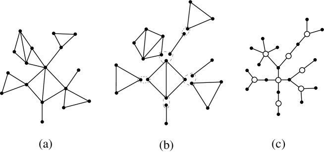
Figure 6. (a) A connected (outerplanar) graph, (b) its block-decomposition, (c) the associated Bv-tree.

4.2. Graphs

We extend here the decomposition principles which we have developed for trees to the more general case of a species of connected graphs, by taking advantage of a well-known “tree-like” decomposition of a connected graph into 2-connected components. (A 2-connected graph is a graph that has at least two vertices and has no separating vertex.) Given a connected graph $G$, a maximal 2-connected subgraph of $G$ is called a block of $G$. The set of vertices of $G$ is denoted $\mathfrak{V}(G)$ and its set of blocks is denoted $\mathfrak{B}(G)$. The Bv-tree of $G$ is the bicolored graph with vertex-set $\mathfrak{V}(G)\cup\mathfrak{B}(G)$ and edges corresponding to the adjacencies between the blocks and the vertices of $G$, see Figure 6. It can be shown that the Bv-tree of $G$ is indeed a tree, see [16, p.10] and [24] for details.

Proposition 15.

Let $\mathcal{G}$ be a species of connected graphs that satisfy the following stability property: “a connected graph is in $\mathcal{G}$ iff all its blocks are in $\mathcal{G}$”. Let $\mathcal{B}$ be the subspecies of graphs in $\mathcal{G}$ that are 2-connected. Then $\mathcal{G}$ admits a decomposition grammar from the species of 2-connected structures $\mathcal{B}^{\prime}$, $\mathcal{B}^{{\circledast}}$, and $(\mathcal{B}^{\prime})^{\circ}$:

$$\left\{\begin{array}[]{rcl}\mathcal{G}^{\circ}&=&X\boldsymbol{\cdot}\mathcal{G}^{\prime}+\mathcal{G}^{{\circledast}}.\\ \mathcal{G}^{\prime}&=&\textsc{Set}\circ\mathcal{K},\quad\mathcal{K}=\mathcal{B}^{\prime}\circ\mathcal{H},\quad\mathcal{H}=X\boldsymbol{\cdot}\mathcal{G}^{\prime},\\ \ \mathcal{G}^{{\circledast}}&=&\mathcal{B}^{{\circledast}}\circledcirc\mathcal{H}+X\boldsymbol{\cdot}\textsc{Set}^{{\circledast}}\circledcirc\mathcal{K},\\ \mathcal{H}^{\circ}&=&X^{\circ}\star\textsc{Set}\circ\mathcal{K}+X\boldsymbol{\cdot}\textsc{Set}^{\circ}\circledcirc\mathcal{K},\ \ \mathcal{K}^{\circ}=(\mathcal{B}^{\prime})^{\circ}\circledcirc\mathcal{H}.\par\end{array}\right.$$ (48)

Hence, if the species of 2-connected structures $\mathcal{B}^{{\circledast}}$ and $\mathcal{B}^{\prime}$ are decomposable (the latter implies that $(\mathcal{B}^{\prime})^{\circ}$ is decomposable), then the cycle-pointed species $\mathcal{G}^{\circ}$ is decomposable as well. More generally, if $Z_{\mathcal{B}^{\prime}}$ and $\overline{Z}_{\mathcal{B}^{{\circledast}}}$ are both solutions of an equation system involving the operations $\{+,\star,\circ,\circledcirc\}$ and basic cycle-index sums, then $Z_{\mathcal{G}^{\circ}}$ is also a solution of such an equation system.

Proof.

The first line of the grammar is obtained as usual by distinguishing whether the marked cycle has length 1 or greater than 1. The second line easily follows from the block decomposition, as shown for instance in [14]. To wit, the marked vertex of a graph in $\mathcal{G}^{\prime}$ is incident to a collection of blocks, and a connected graph is possibly attached at each non-marked vertex of these blocks. Let us prove the third line in a similar way as for free trees (Claim 10). Consider a graph $G$ in $\mathcal{G}^{\prime}$, and let $T$ be the Bv-tree of $G$. Clearly the Bv-tree of a graph has less structure than the graph itself, so any automorphism of $G$ induces an automorphism on $T$. In particular $T$ is a symmetric cycle-pointed tree, hence it has a center of symmetry that either corresponds to a block or to a vertex of $G$. The species of graphs in $\mathcal{G}^{{\circledast}}$ whose center of symmetry in the Bv-tree is a vertex (a block) is denoted $(\mathcal{G}^{{\circledast}})_{\mathrm{v}}$ ($(\mathcal{G}^{{\circledast}})_{\mathrm{B}}$, resp.). Let $\mathcal{G}_{\mathrm{v}}$ ($\mathcal{G}_{\mathrm{B}}$) be the species of graphs in $\mathcal{G}$ with a marked vertex (block, resp.) that is colored blue. Then clearly $\mathcal{G}_{\mathrm{v}}=X\boldsymbol{\cdot}\mathcal{G}^{\prime}$ and $\mathcal{G}_{\mathrm{B}}=\mathcal{B}\circ(X\boldsymbol{\cdot}\mathcal{G}^{\prime})$. Hence, following the notations introduced in the grammar, $\mathcal{G}_{\mathrm{v}}=\mathcal{H}=X\boldsymbol{\cdot}\textsc{Set}\circ\mathcal{K}$ and $\mathcal{G}_{\mathrm{B}}=\mathcal{B}\circ\mathcal{H}$. Note that the structures in $(\mathcal{G}^{{\circledast}})_{\mathrm{v}}$ ($(\mathcal{G}^{{\circledast}})_{\mathrm{B}}$) are the graphs in $\mathcal{G}_{\mathrm{v}}\ \!\!^{{\circledast}}$ ($\mathcal{G}_{\mathrm{B}}\ \!\!^{{\circledast}}$) such that the center of symmetry of the associated Bv-tree is the blue vertex (block, resp.). It is easy to check, in a similar way as for free trees, that this property holds only for the graphs of $\mathcal{G}_{\mathrm{v}}\ \!\!^{{\circledast}}$ that are in $X\boldsymbol{\cdot}\textsc{Set}^{{\circledast}}\circledcirc\mathcal{K}$ and only for the graphs of $\mathcal{G}_{\mathrm{B}}\ \!\!^{{\circledast}}$ that are in $\mathcal{B}^{{\circledast}}\circledcirc\mathcal{H}$. Finally, the 4th line, which is necessary to have only species of 2-connected structures as terminal species, is obtained from the second line by applying the derivation rules (Proposition 6). ∎

Remark 4.4.

Trees are exactly connected graphs where each block is an edge. In other words, the species $\mathcal{F}$ of free trees is the species $\mathcal{G}$ of connected graphs formed from the species $\mathcal{B}=\mathcal{L}$ (the one-element species that consists of the link graph). One easily checks that, in that case, the grammar (48) for $\mathcal{G}$ is equivalent to the grammar (34) for free trees.

4.2.1. Cacti graphs

Cacti graphs form an important class of graphs that have several algorithmic applications. They consist of cycles attached together in a tree-like fashion; in other words, the species of cacti graphs arises from the species of 2-connected structures as $\mathcal{B}=\mathcal{L}+\mathcal{P}$ where $\mathcal{L}$ is the species of the link graph and $\mathcal{P}$ is the speices of polygons with at least 3 edges (i.e., $\mathcal{B}$ is the species of polygons where one allows the degenerated 2-sided polygon).

Thanks to the grammar (48), the unlabeled enumeration of connected cacti graphs reduces to the calculation of the cycle-index sums for the species of 2-connected structures $\mathcal{B}^{\prime}$ and $\mathcal{B}^{{\circledast}}$ (the cycle-index sum $\overline{Z}_{(\mathcal{B}^{\prime})^{\circ}}$ is also required, but it can directly be deduced from $Z_{\mathcal{B}^{\prime}}$ by differentiation). Since the 2-connected cacti graphs are polygons, the possible automorphisms are from the dihedral group. In addition, the presence of a marked vertex (for $\mathcal{B}^{\prime}$) or cycle (for $\mathcal{B}^{{\circledast}}$) restricts the symmetries. For instance, if a structure in $\mathcal{B}^{\prime}$ has a marked (unlabeled) vertex $v$, then the automorphisms have to fix $v$; there are only two such symmetries for each polygon, the identity and the unique reflection whose axis passes by $v$. Accordingly, we have two terms in the expression of $Z_{\mathcal{B}^{\prime}}$ below, the first one for the identity, and the second one for reflections (where one distinguishes whether the polygon has odd or even length).

$$Z_{\mathcal{B}^{\prime}}=\frac{1}{2}\frac{s_{1}}{1-s_{1}}+\frac{1}{2}\frac{s_{1}+s_{2}}{1-s_{2}}$$

For $\mathcal{B}^{{\circledast}}$, all symmetries must be nontrivial and have to respect the marked cycle. These symmetries are of two types: rotation and reflection, which yields the two main terms in the expression of $\overline{Z}_{\mathcal{B}^{{\circledast}}}$ below.

$$\overline{Z}_{\mathcal{B}^{{\circledast}}}=\sum_{r\geq 2}\frac{\phi(r)}{2}\frac{t_{r}}{1-s_{r}}+\frac{t_{2}(s_{1}^{2}+2s_{1}+1)}{2(1-s_{2})^{2}}$$

The expressions for $Z_{\mathcal{B}^{\prime}}$ and $\overline{Z}_{\mathcal{B}^{{\circledast}}}$ can be used to enumerate unlabeled cacti graphs. We just have to translate (using the computation rules in Remark 2.1 and Remark 3.3) the grammar (48) – applied to the species of cacti graphs – into an equation system satisfied by the corresponding ordinary generating functions.

Proposition 16 (enumeration of unlabeled cacti graphs).

The ordinary generating function $c(x)=\sum_{n}c_{n}x^{n}$ of unlabeled cacti graphs counted with respect to the number of vertices satisfies

$$xc^{\prime}(x) = H(x)+I(x),$$

$$H(x) = x\exp\Big{(}\sum_{r\geq 1}\frac{K(x^{r})}{r}\Big{)},\ \ \mathrm{with}\ K(x)=\frac{1}{2}\frac{H(x)}{1-H(x)}+\frac{1}{2}\frac{H(x)+H(x^{2})}{1-H(x^{2})},$$

$$I(x) = \sum_{r\geq 2}\frac{\phi(r)}{2}\frac{x^{r}H^{\prime}(x^{r})}{1-H(x^{r})}+\frac{x^{2}H^{\prime}(x^{2})(H(x)^{2}+2H(x)+1)}{2(1-H(x^{2}))^{2}}+H(x)\sum_{r\geq 2}x^{r}K^{\prime}(x^{r}),$$

from which one can extract the counting coefficients $c_{n}$ (after firstly extracting the coefficients of $H(x)$):

$$xc^{\prime}(x)=1\cdot\mathbf{1}\cdot x+2\cdot\mathbf{1}\cdot x^{2}+3\cdot\mathbf{2}\cdot x^{3}+4\cdot\mathbf{4}\cdot x^{4}+5\cdot\mathbf{9}\cdot x^{5}+6\cdot\mathbf{23}\cdot x^{6}+7\cdot\mathbf{63}\cdot x^{7}+\ldots.$$

4.2.2. Outerplanar graphs

Outerplanar graphs are graphs that can be drawn in the plane so that all vertices are incident to the outer face. They form a fundamental subspecies of the species of planar graphs, which already captures some difficulties of the species of all planar graphs; for example, the convergence rate of sampling procedures using the Markov Chain approach is not known. However, outerplanar graphs are easier to tackle with the decomposition approach. For enumeration, we use the well-known property that 2-connected outerplanar graphs, except for the one-edge graph, have a unique hamiltonian cycle. Hence, the species $\mathcal{B}$ of 2-connected outerplanar graphs can be identified with the species of dissections of a polygon (allowing a degenerated 2-sided dissection). This time, to obtain the cycle index sums $Z_{\mathcal{B}^{\prime}}$ and $\overline{Z}_{\mathcal{B}^{{\circledast}}}$, we have to count not polygons (as for cacti graphs) but dissections of a polygon under the action of the dihedral group. We only sketch the method here (the principles for counting such dissections are well known, going back to earlier articles of Read [30], see also [3] for more detailed calculations).

For each type of symmetry (rotation or reflection), one considers the “quotient dissection”, as shown in Figure 7. Notice that a dissection fixed by a rotation has either a central edge (only for the rotation of order two) or a central face. In case of a central edge $e$, it turns out to be more convenient to “double” $e$, so as to always have a central face before taking the quotient. Thus, the quotient dissection has a marked face (the quotient of the central face) that might have degree one (only for rotations of order at least three) or two (only for rotations of order at least two). Concerning quotient dissections under a reflection, there are two special vertices $v_{1}$ and $v_{2}$ on the boundary (the intersections of the original polygon with the reflection-axis), and there might be some other special vertices, all of degree three, on the boundary path from $v_{1}$ to $v_{2}$; see Figure 7.

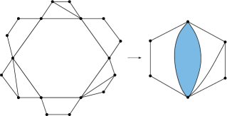
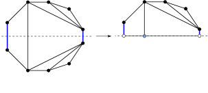
Figure 7. Left (Right, resp.): the quotient of a dissection under a rotation (reflection, resp.).

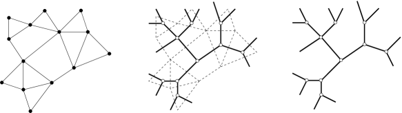
Figure 8. The dual tree of a dissection.

The second ingredient is to take the dual of such quotient dissections in order to obtain plane trees, which are easier to decompose and to count. Notice that if the rotation is the identity rotation, then the associated plane tree is in the species $\mathcal{F}$ of plane trees with no vertex of degree two. Notice also that each leaf of the tree corresponds to a vertex of the dissection; see Figure 8 for an example. The generating function of $\mathcal{F}$ with respect to the number of leaves satisfies

$$F(x)=x+\frac{F(x)^{2}}{1-F(x)}.$$ (49)

To calculate $Z_{\mathcal{B}^{\prime}}$ and $Z_{\mathcal{B}^{{\circledast}}}$, one computes separately the contributions of rotations and reflections to $Z_{\mathcal{B}^{\prime}}$ and to $Z_{\mathcal{B}^{{\circledast}}}$. In each case, using duality, the contribution is easily expressed in terms of the series $F(x)$. All calculations done, one finds:

$$Z_{\mathcal{B}^{\prime}}=\frac{1}{2}\big{(}F(s_{1})+(s_{1}+s_{2})P(s_{2})\big{)},\ \ \ \ \overline{Z}_{\mathcal{B}^{{\circledast}}}=\frac{1}{2}\sum_{r\geq 2}\phi(r)t_{r}G(s_{r})+\frac{1}{2}t_{2}\big{(}1+s_{1}^{2}Q(s_{2})+2s_{1}R(s_{2})+S(s_{2})\big{)},$$

where

$\displaystyle G(x)=\frac{F^{\prime}(x)}{1-F(x)},\ \ P(x)=\frac{1}{x}\frac{F(x)}{1-2F(x)},$

$\displaystyle Q(x)=\frac{\mathrm{d}}{\mathrm{d}x}P(x),\ \ R(x)=\frac{\mathrm{d}}{\mathrm{d}x}(xP(x)),\ \ S(x)=\frac{\mathrm{d}}{\mathrm{d}x}(x^{2}P(x)).$

Similarly as for cacti graphs, the expressions for $Z_{\mathcal{B}^{\prime}}$ and $\overline{Z}_{\mathcal{B}^{{\circledast}}}$ make it possible to enumerate unlabeled connected outerplanar graphs. Translating the grammar (48) into an equation system on the corresponding generating functions, we obtain the following.

Proposition 17 (Enumeration of unlabeled connected outerplanar graphs).

The ordinary generating function $o(x)=\sum_{n}o_{n}x^{n}$ of unlabeled connected outerplanar graphs counted with respect to the number of vertices satisfies the system:

$$xo^{\prime}(x) = H(x)+I(x),$$

$$H(x) = x\exp\Big{(}\sum_{r\geq 1}\frac{K(x^{r})}{r}\Big{)},\ \ \mathrm{with}\ K(x)=\frac{1}{2}F(H(x))+\frac{1}{2}(H(x)+H(x^{2}))\cdot P(H(x^{2})),$$

$$I(x) = \frac{1}{2}\sum_{r\geq 2}\phi(r)x^{r}H^{\prime}(x^{r})G(H(x^{r}))+H(x)\sum_{r\geq 2}x^{r}K^{\prime}(x^{r})$$

$$+\frac{1}{2}x^{2}H^{\prime}(x^{2})\big{(}1+H(x)^{2}Q(H(x^{2}))+2H(x)R(H(x^{2}))+S(H(x^{2}))\big{)},$$

where the series $F$, $G$, $P$, $Q$, $R$, $S$ are defined above. One extracts from this system (extracting firstly the coefficients in $F$, $Q$, $R$, $S$, then in $H$ and $K$, then in $I$) the counting coefficients $o_{n}$:

$$xo^{\prime}(x)=1\cdot\mathbf{1}\cdot x+2\cdot\mathbf{1}\cdot x^{2}+3\cdot\mathbf{2}\cdot x^{3}+4\cdot\mathbf{5}\cdot x^{4}+5\cdot\mathbf{13}\cdot x^{5}+6\cdot\mathbf{46}\cdot x^{6}+7\cdot\mathbf{172}\cdot x^{7}+\ldots.$$

4.3. Maps

A map is a planar graph embedded on a sphere up to isotopic deformation, i.e., it is a planar graph together with a cyclic order of the neighbors around each vertex. There is a huge literature on maps since the pioneering work of Tutte [33]. As we show next, the decomposition grammar (48) for maps is actually simpler than for graphs, and it allows us to enumerate (unrooted unlabeled) 2-connected maps in terms of not necessarily connected maps. To write down the grammar, it turns out to be more convenient to take half-edges as atoms instead of vertices. Denote by $\mathcal{M}$ the species of maps – so $\mathcal{R}:=\mathcal{Z}\boldsymbol{\cdot}\mathcal{M}^{\prime}$ is the species of rooted maps (maps with a marked half-edge) – and by $\mathcal{B}$ the species of 2-connected maps (the loop-map is considered as 2-connected).

Proposition 18.

The species of rooted maps and symmetric cycle-pointed maps (in each length $\ell\geq 2$ of the marked cycle) have the following recursive specification over the corresponding species of rooted and cycle-pointed 2-connected maps.

$$\left\{\begin{array}[]{rcl}\mathcal{R}$\!\!\!$&=&$\!\!\!$\mathcal{K}\boldsymbol{\cdot}\textsc{Seq}\circ\mathcal{K},\ \ \mathcal{K}=X\boldsymbol{\cdot}\mathcal{B}^{\prime}\circ\mathcal{H},\ \ \mathcal{H}=X\boldsymbol{\cdot}(1+\mathcal{R})\;,\\ \mathcal{M}^{\circ}_{(\ell)}$\!\!\!$&=&$\!\!\!$\mathcal{B}^{\circ}_{(\ell)}\circledcirc\mathcal{H}+\textsc{Cyc}^{\circ}_{(\ell)}\circledcirc\mathcal{K}\ \mathrm{for}\ \ell\geq 2\;.\end{array}\right.$$ (50)

Proof.

The arguments are similar to the proof for graphs (Proposition 15). The only difference is that one takes the embedding into account, hence corners (which are in one-to-one correspondence with half-edges for a given map) play for maps a similar role as vertices do for graphs, and a Set construction typically becomes a Cyc construction here. Let us comment here on the decomposition for symmetric cycle-pointed maps (the one for rooted maps is well known, see [33]). One has

$$\mathcal{M}^{{\circledast}}=\mathcal{B}^{{\circledast}}\circledcirc\mathcal{H}+\textsc{Cyc}^{{\circledast}}\circledcirc\mathcal{K},$$ (51)

where the first (second) term takes account of the maps whose center of symmetry – for the associated block-decomposition tree – is a block (vertex, respectively). Further simplification is possible, since a rooted map has only the identity as automorphism. Hence, the species of rooted maps $\mathcal{H}$ and $\mathcal{K}$ satisfy $\mathcal{H}^{\circ}=\mathcal{H}^{\circ}_{(1)}$ and $\mathcal{K}^{\circ}=\mathcal{K}^{\circ}_{(1)}$. Thus, Equation (51) can be “sliced” into a collection of equations, one for each length $\ell\geq 2$ of the marked cycle. ∎

An important property of any map automorphism – as shown by Liskovets [22] – is that all its cycles have the same length $\ell$, which is also the order of the automorphism. Hence, the number of half-edges of a cycle-pointed map with a marked cycle of length $\ell$ is divisible by $\ell$. For $\ell\geq 1$, denote by $M_{(\ell)}(x)$ ($B_{(\ell)}(y)$) the series counting unlabeled cycle-pointed maps (2-connected maps, respectively), according to the number of half-edges, divided by $\ell$. In particular, $R(x):=M_{(1)}(x)$ and $S(x):=B_{(1)}(x)$ are the series counting rooted maps and rooted 2-connected maps, respectively. We clearly have

$$\overline{Z}_{\mathcal{M}^{\circ}_{(\ell)}}=\frac{t_{\ell}}{s_{\ell}}M_{(\ell)}(s_{\ell}),\ \ \ \ \overline{Z}_{\mathcal{B}^{\circ}_{(\ell)}}=\frac{t_{\ell}}{s_{\ell}}B_{(\ell)}(s_{\ell})\;.$$

Given this simplification, the grammar (50) is translated into the following system relating the series counting species of maps and species of 2-connected maps:

$$R(x) = \frac{K(x)}{1-K(x)},\ \ \ \ H(x)=x(1+R(x)),\ \ \ \ K(x)=\frac{x}{H(x)}S(H(x)),$$ (52)

$$M_{(\ell)}(x) = \frac{xH^{\prime}(x)}{H(x)}B_{(\ell)}(H(x))+\phi(\ell)\frac{xK^{\prime}(x)}{1-K(x)}\ \ \mathrm{for}\ \ell\geq 2.$$ (53)

In the case of maps, the decomposition grammar is used in the other direction, i.e., one obtains the enumeration of (unrooted) 2-connected maps from maps. Indeed, unconstrained maps are easier to count, by a method of quotient [22] similar to the one we have used for counting dissections in Section 4.2.2.

Let us first review (from Tutte [33]) how one obtains an expression for the series $S(y)$ counting rooted 2-connected maps from an expression for the series $R(x)$ counting rooted maps. One starts from the following expression of $R(x)$:

$$R(x)=\frac{\beta(2-9\beta)}{(1-3\beta)^{2}},\ \ \ \mathrm{with}\ \ \beta=\beta(x)\ \ \mathrm{specified\ by}\ \ \beta=x^{2}+3\beta^{2}.$$ (54)

Next, notice that the change of variable $y=H(x)=x(1+R(x))$ between rooted maps and rooted 2-connected maps is such that $y^{2}$ is also rational in $\beta$:

$$y^{2}=x^{2}(1+R(x))^{2}=\beta\frac{(1-4\beta)^{2}}{(1-3\beta)^{3}}.$$

Equivalently:

$$y^{2}=\eta(1-\eta)^{2},\ \ \mathrm{where}\ \ \eta:=\frac{\beta}{1-3\beta},$$

so the dependence between $\eta$ and $\beta$ is invertible: $\beta=\eta/(1+3\eta)$. Notice also from (52) that

$$S(y)=\frac{H(x)}{x}K(x)=(1+R(x))K(x)=R(x)=\frac{\beta(2-9\beta)}{(1-3\beta)^{2}}.$$

Replacing $\beta$ by $\eta/(1+3\eta)$, one gets

$$S(y)=\eta(2-3\eta),\ \ \mathrm{with}\ \eta=\eta(y)\ \mathrm{specified\ by}\ \eta=\frac{y^{2}}{(1-\eta)^{2}},$$

which can also be written as

$$S(y)=\overline{S}(y^{2}),\ \ \mathrm{with}\ \overline{S}(y)=\overline{\eta}(2-3\overline{\eta}),\ \mathrm{and}\ \overline{\eta}:=\overline{\eta}(y)\ \mathrm{specified\ by}\ \overline{\eta}=\frac{y}{(1-\overline{\eta})^{2}}.$$ (55)

In a similar way, if two series $f(x)=g(y)$ are related by the change of variables $y=H(x)$ and if $f(x)$ is rational in $\beta(x)$, then $g(y)$ is rational in $\eta(y)$ (replacing $\beta$ by $\eta/(1+3\eta)$). For instance, for $\ell\geq 3$, it has been shown by Liskovets using the quotient method (see [12] for the reformulation on series) that

$$M_{(\ell)}(x)=\phi(\ell)\frac{6\beta(x)}{1-6\beta(x)}.$$

Since $H(x)/x=1+R(x)$ and $K(x)=R(x)/(1+R(x))$ are rational in $\beta$, as well as $xH^{\prime}(x)$ and $xK^{\prime}(x)$ (noticing that $x\mathrm{d}f/\mathrm{d}x=2x^{2}\mathrm{d}f/\mathrm{d}x^{2}=2\beta(1-3\beta)\cdot(\mathrm{d}f/\mathrm{d}\beta)/(\mathrm{d}x^{2}/\mathrm{d}\beta)$), one finds from (53) a rational expression in $\beta$ for the series $B_{(\ell)}(H(x))$. Replacing $\beta$ by $\eta/(1+3\eta)$ in that expression, one finally gets:

$$B_{(\ell)}(y)=\phi(\ell)\frac{2\eta(y)}{1-3\eta(y)}\ \ \mathrm{for}\ \ell\geq 3,$$

which can also be written as

$$B_{(\ell)}(y)=\phi(\ell)G(y^{2})\ \ \mathrm{for}\ \ell\geq 3,\ \mathrm{with}\ G(y)=\frac{2\overline{\eta}(y)}{1-3\overline{\eta}(y)}.$$ (56)

In a similar way, starting from the expression (given in [12])

$$M_{(2)}(x)=-1+\frac{1-2\beta(x)}{(1-6\beta(x))(1-3\beta(x))}+x\cdot\frac{2}{(1-6\beta(x))(1-3\beta(x))},$$

one obtains the following expression for $B_{(2)}(y)$:

$$B_{(2)}(y)=\frac{\eta(y)(3-\eta(y))}{1-3\eta(y)}+y\frac{2}{1-3\eta(y)},$$

which can also be written as

$$B_{(2)}(y)=P(y^{2})+yQ(y^{2}),\mathrm{with}\ P(y)=\frac{\overline{\eta}(y)(3-\overline{\eta}(y))}{1-3\overline{\eta}(y)}\ \mathrm{and}\ Q(y)=\frac{2}{1-3\overline{\eta}(y)}.$$ (57)

Proposition 19 (counting unrooted 2-connected maps, recover [23]).

The number $t_{n}$ of (unrooted unlabeled) 2-connected maps with $n$ edges satisfies:

$$t_{n}=\frac{1}{2n}\Big{(}s_{n}+u_{n}+\frac{1}{2}\sum_{k|n,k\neq n}\phi(n/k)\cdot(9k^{2}-9k+1)s_{k}\Big{)},$$ (58)

where $\displaystyle s_{n}=\frac{2(3n-3)!}{n!(2n-1)!}$, $\displaystyle u_{n}=\frac{n(n+1)}{2}s_{(n+1)/2}$ if $n$ is odd, and $\displaystyle u_{n}=\frac{(3n-4)n}{8}s_{n/2}$ if $n$ is even.

Proof.

Cycle-pointing ensures that the generating function $\widetilde{\mathcal{B}^{\circ}}(y)=\sum_{n}2nt_{n}y^{2n}$ satisfies

$$\widetilde{\mathcal{B}^{\circ}}(y)=S(y)+B_{(2)}(y^{2})+\sum_{\ell\geq 3}B_{(\ell)}(y^{\ell})=S(y)+\Big{(}B_{(2)}(y^{2})-G(y^{4})\Big{)}+\sum_{\ell\geq 2}\phi(\ell)G(y^{2\ell}).$$

Extracting the coefficient $[y^{2n}]$ in this equation yields

$$2nt_{n}=s_{n}+u_{n}+\sum_{\ell\geq 2,\ell|n}\phi(\ell)v_{n/\ell}=s_{n}+u_{n}+\sum_{k|n,k\neq n}\phi(n/k)v_{k},$$ (59)

where $s_{n}=[y^{n}]\overline{S}(y)$, $v_{n}=[y^{n}]G(y)$, $u_{n}=[y^{n}](B_{(2)}(y)-G(y^{2}))$, which is $[y^{n/2}]P(y)-v_{n/2}$ if $n$ is even and $y^{(n-1)/2}Q(y)$ if $n$ is odd. Notice that the series $\overline{S}(y)$, $G(y)$, $P(y)$, and $Q(y)$ are rational in the simple series $\overline{\eta}(y)=y/(1-\overline{\eta}(y))^{2}$. Hence the Lagrange inversion formula [2, Section 3.1] allows us to extract exact formulas for the coefficients $s_{n}$, $v_{n}$, and $u_{n}$. Substituting these exact expressions in (59), one obtains the announced formula for $t_{n}$. ∎

The enumeration of unrooted 2-connected maps has first been done by Liskovets and Walsh [23] using the quotient method in a quite involved way. More recently, the counting formula has been recovered in [12] using a method of extraction at a center of symmetry on quadrangulations. What we do here is equivalent to [12], but the cycle-pointed framework allows us to write the equations on generating functions in a more systematic way.

4.4. Asymptotic enumeration

Cycle-pointing makes it possible to easily obtain an asymptotic estimate for the coefficients counting the number of unlabeled structures from a species, provided that the singular behavior of the OGS counting the associated species of rooted unlabeled structures is known.

We illustrate the method on free trees. Let $R(x)$ be the OGS of rooted unlabeled nonplane trees, which is specified by $R(x)=x\exp(\sum_{i\geq 1}R(x^{i})/i)$. It is well known that $R(x)$ has a dominant singularity $\rho<1$ of the square-root type [10, VII.5]. That is, in the slit complex neighborhood $D_{\epsilon}:=\{x\;|\;x-\rho\notin\mathbb{R}_{+}\ \mathrm{and}\ |x-\rho|<\epsilon\}$ we have the expansion

$$R(x)=1-a\ \!X+o(X),\ \ \mathrm{where}\ X=\sqrt{1-x/\rho},$$ (60)

which yields – using transfer theorems of analytic combinatorics [10, VI] – the asymptotic estimate

$$R_{n}\sim c\,n^{-3/2}\,\rho^{-n},\ \ \mathrm{where}\ c=\frac{a}{2\sqrt{\pi}}\approx 0.43922,\ \ \rho\approx 0.33832,$$ (61)

for the number of rooted unlabeled nonplane trees with $n$ vertices.

To obtain a similar estimate for free trees, we consider the OGS $P(x)$ of cycle-pointed nonplane trees and start from the expression of $P(x)$ obtained in Proposition 11:

$$P(x)=x^{2}R^{\prime}(x^{2})+\big{(}1+\sum_{\ell\geq 2}x^{\ell}R^{\prime}(x^{\ell})\big{)}R(x).$$

Notice that, since $\rho<1$, the series $A:=x^{2}R^{\prime}(x^{2})$ and $B:=1+\sum_{\ell\geq 2}x^{\ell}R^{\prime}(x^{\ell})$ are analytic at $x=\rho$, and the value at $x=\rho$ of $B$ is the positive constant

$$b:=1+\sum_{\ell\geq 2}\rho^{\ell}R^{\prime}(\rho^{\ell}).$$ (62)

Therefore, from the singular expansion (60) of $R(x)$, we obtain

$$P(x)=P(\rho)-ab\ \!X+o(X)\;.$$ (63)

Let us simplify further the positive constant $b=B(\rho)$. First, by deriving the equation that specifies $R(x)$, one obtains $xR^{\prime}(x)=R(x)\big{(}1+\sum_{i\geq 1}x^{i}R^{\prime}(x^{i})\big{)}$, which yields

$$B(x)R(x)=xR^{\prime}(x)(1-R(x))\;.$$

By deriving the singular expansion of $R(x)$, one obtains

$$R^{\prime}(x)=\frac{a}{2\rho}X^{-1}+o(X^{-1})\;,$$

hence $xR^{\prime}(x)(1-R(x))$ converges to $a^{2}/2$ as $x\to\rho$, i.e., $b=a^{2}/2$.

Proposition 20 (asymptotic enumeration of free trees).

The number $F_{n}$ of unlabeled free trees with $n$ vertices satisfies

$$F_{n}\sim(2\pi c^{3})n^{-5/2}\rho^{-n},$$ (64)

where $c$ is the constant and $\rho^{-1}$ is the growth ratio in the estimate (61) for rooted nonplane trees ($R_{n}\sim c\ \!n^{-3/2}\rho^{-n}$).

Proof.

From the singular expansion (63) of $P(x)$ we obtain (again by the transfer theorems of singularity analysis)

$$x^{n}[P(x)]\sim\frac{ab}{2\sqrt{\pi}}n^{-3/2}\rho^{-n}\;.$$

Using $c=a/(2\sqrt{\pi})$ and $b=a^{2}/2$, we have $ab/(2\sqrt{\pi})=2\pi c^{3}$. Finally, Theorem 5 (unbiased pointing) yields $F_{n}=\frac{1}{n}[x^{n}]P(x)$, so $F_{n}\sim(2\pi c^{3})n^{-5/2}\rho^{-n}$. ∎

It is also possible to get the estimate of $F_{n}$ from Otter’s dissimilarity equation (or from the dissymmetry theorem). However, we find that cycle-pointing provides a more transparent explanation why the asymptotic estimate of the coefficients $F_{n}$ counting unlabeled structures from an unrooted “tree-like” species $\mathcal{F}$ is of the universal type $cn^{-5/2}\rho^{-n}$. The argument is very simple:

• The OGS $P(x)$ of the cycle-pointed species $\mathcal{F}^{\circ}$ is positively expressed in terms of the OGS of the rooted species, which has a square-root dominant singularity. Therefore, $P(x)$ inherits the same singularity and singularity type (square-root).

• Transfer theorems of singularity analysis ensure that a square-root dominant singularity yields an asymptotic estimate in $cn^{-3/2}\rho^{-n}$ for the coefficients $[x^{n}]P(x)$. Since $F_{n}=\frac{1}{n}[x^{n}]P(x)$, one gets $F_{n}\sim c\ \!n^{-5/2}\,\rho^{-n}$.

This strategy applies to all species of trees encountered in this section, as well as to cacti graphs and connected outerplanar graphs (in all cases one starts from the singular expansion of the OGS counting the corresponding rooted species).

5. Application to Random Generation

Recently, so-called Boltzmann samplers have been introduced by Duchon et al [9] as a general method to efficiently (typically in linear time) generate uniformly at random combinatorial structures that admit a decomposition. In contrast to the more costly recursive method of sampling [25], which is based on counting coefficients of the recursive decomposition, Boltzmann samplers are primarily based on generating functions. Until now Boltzmann samplers were developed in the labeled setting [9] and partially in the unlabeled setting [13].

In this section we provide a more complete method in the unlabeled setting. In order to deal with the substitution construction and the cycle-pointing operator (which are not covered in [13]), we have to describe samplers not solely based on ordinary generating functions, but on cycle index sums – also known as Pólya operators. Therefore we call these random generators Pólya-Boltzmann samplers.

With these refined samplers we are able to design in a systematic way (via specific generation rules) a Pólya-Boltzmann sampler for species that admit a recursive decomposition, thereby allowing in the decomposition all operators that have been described in this article. When specialized suitably, a Pólya-Boltzmann sampler reduces to an ordinary Boltzmann sampler, hence it provides a uniform random sampler for species of unlabeled structures. In particular, we obtain highly efficient random generators for the species in Section 4: for trees, cacti graphs, outerplanar graphs, etc.

5.1. Ordinary Boltzmann Samplers

Let $\mathcal{A}$ be a species of structures, and let $\widetilde{\mathcal{A}}(x)$ be the ordinary generating series for $\mathcal{A}$. A real number $x>0$ is said to be admissible iff the sum defining $\widetilde{\mathcal{A}}(x)$ converges ($x$ within the disk of convergence of the series). Given a fixed admissible value $x>0$, an ordinary Boltzmann sampler for unlabeled structures from ${\mathcal{A}}$ is a random generator $\Gamma\widetilde{\mathcal{A}}(x)$ that draws each structure $\gamma\in\widetilde{\mathcal{A}}$ with probability

$$\mathbb{P}_{x}(\gamma)=\frac{x^{|\gamma|}}{\widetilde{\mathcal{A}}(x)}\;.$$ (65)

Notice that this distribution has the fundamental property to be uniform, i.e., any two unlabeled structures of the species with the same size have the same probability.

5.1.1. Automatic rules to design Boltzmann samplers

As described in [9], there are simple rules to assemble Boltzmann samplers for the two classical constructions Sum and Product ($\mathrm{Bern}(p)$ stands for a Bernoulli law, returning “true” with probability $p$ and “false” with probability $1-p$).

$\mathcal{C}=\mathcal{A}+\mathcal{B}$.	$\Gamma\widetilde{\mathcal{C}}(x)$:	if $\mathrm{Bern}(\widetilde{\mathcal{A}}(x)/\widetilde{\mathcal{C}}(x))$ return $\Gamma\widetilde{\mathcal{A}}(x)$ else return $\Gamma\widetilde{\mathcal{B}}(x)$
$\mathcal{C}=\mathcal{A}\ \!\boldsymbol{\cdot}\ \!\mathcal{B}$.	$\Gamma\widetilde{\mathcal{C}}(x)$:	return $(\Gamma\widetilde{\mathcal{A}}(x),\Gamma\widetilde{\mathcal{B}}(x))$ {independent calls}

These rules can be used recursively. For instance, the species $\mathcal{T}$ of rooted binary trees satisfies

$$\mathcal{T}=X+\mathcal{T}\boldsymbol{\cdot}\mathcal{T},$$ (66)

which translates to the following Boltzmann sampler:

$\Gamma\widetilde{\mathcal{T}}(x)$:

if $\mathrm{Bern}\left(\frac{x}{\widetilde{T}(x)}\right)$ return leaf else return $(\Gamma\widetilde{\mathcal{T}}(x),\mathrm{node},\Gamma\widetilde{\mathcal{T}}(x))$.

5.1.2. The complexity model

Typically, when $\mathcal{F}$ has a recursive specification over the species $\mathcal{A}_{1},\dots,\mathcal{A}_{l}$, then our sampling procedure $\Gamma\widetilde{\mathcal{F}}(x)$ will require that we can evaluate the ordinary generating functions for $\mathcal{A}_{1},\dots,\mathcal{A}_{l}$ at real values $x$. Indeed, for a species $\mathcal{F}$ defined as $\mathcal{A}_{1}+\mathcal{A}_{2}$, each Bernoulli choice requires to draw a uniform value in $[0,1]$ and compare it with a ratio of the form $\widetilde{\mathcal{A}_{1}}(x)/\widetilde{\mathcal{F}}(x)$. In the following we work with the complexity model where we assume that there exists an oracle that provides at unit cost the exact values of these generating functions at $x$, and that a random number in $[0,1]$ can be generated and compared with a fixed value such as $\widetilde{\mathcal{A}}(x)/\widetilde{\mathcal{C}}(x)$ in constant time as well. We will refer to this complexity model as the real-arithmetic complexity model in the following.

The model is justified since in many applications we obtain expressions for the ordinary generating series that allow a rapid numeric evaluation of those series at given values, for example with the Newton method. Then, in practice, one works at a fixed precision, say $N$ bits (typically $N=64$, correspondingly roughly to 20 decimal digits).

Let us mention that the Boltzmann samplers for the constructions Multiset and Cycle—as given in [13] and recovered in a more general framework here—require typically the values of the generating functions not only at $x$, but at all powers $x^{i}$. Since combinatorial species often have exponential growth rate (which is the case for all examples presented here), the dominant singularity $\rho$ satisfies $\rho<1$, hence $x\leq\rho<1$. Therefore the values $\widetilde{\mathcal{A}}(x^{i})$ decrease exponentially fast with $i$. When working at fixed precision of $N$ bits, one can thus discard the powers greater than $k=N/\log_{2}(1/\rho)$ and assume that the oracle provides the evaluations of the generating functions at $x,x^{2},\ldots,x^{k}$. For a more detailed study and implementation of the evaluation procedures we refer to the recent article by Pivoteau, Salvy, and Soria [27].

Proposition 21 (Duchon et al. [9]).

Let $\mathcal{F}$ be a species that can be decomposed recursively from $\{\mathbf{1},X\}$ in terms of the constructions $\{+,\boldsymbol{\cdot}\}$ (this is meant analogous to but more restricted than Definition 2.7). Then one can obtain in a systematic way (from the recursive specification) an ordinary Boltzmann sampler $\Gamma\widetilde{\mathcal{F}}(x)$ for $\mathcal{F}$. In addition, in the real-arithmetic complexity model, $\Gamma\widetilde{\mathcal{F}}(x)$ operates in linear time in the size of the output.

This result was recently extended in [13] to other constructions, such as the Multiset and Cycle constructions (and their counterpart with fixed number of components). In this section we extend this result to the substitution construction, and to the cycle-pointed constructions. It follows that any species that is cycle-pointed decomposable over species where we already have a Pólya-Boltzman sampler also has a Pólya-Boltzman sampler.

Remark 5.1.

Note that in the general results on sampling we consider species up to isomorphism. Theoretically, this is a necessary assumption, since isomorphisms between species might in artificial examples be non-effective. However, in all the presented examples and applications in this article, the isomorphisms between species are straightforward and efficiently computable. The effectiveness of isomorphisms between the output species of the sampling procedures and the actual species are actually more related to the question how combinatorial structures are represented on a computer, and in particular they do not concern the complexity of the sampling task itself.

5.1.3. Targeting Boltzmann samplers

Boltzmann samplers often lead to very efficient exact-size and approximate-size random samplers. In order to draw unlabeled structures uniformly at random from a species $\mathcal{A}$ at (in case of exact-size sampling) or around (in case of approximate-size sampling) a target-size $n$, one simply repeats calling the Boltzmann sampler $\Gamma\widetilde{\mathcal{A}}(x)$ – with a suitably chosen value of $x$ – until the size of the output is $n$ (exact-size sampling) or is in $[n(1-\epsilon),n(1+\epsilon)]$ (approximate-size sampling), where $\epsilon$ is a tolerance-parameter fixed by the user. It turns out that for a wide class of species, which covers the species encountered in Section 4 (trees, cacti graphs, outerplanar graphs), this method works very well, as proved in [9].

Proposition 22 (Duchon et al [9]).

Let $\mathcal{F}$ be a species such that asymptotically

$$|\widetilde{\mathcal{F}}_{n}|\sim c\;n^{-3/2}\;\rho^{-n}$$

for some positive constant $c$, and where $\rho$ is the radius of convergence of $\widetilde{\mathcal{F}}(x)$, assuming that $\widetilde{\mathcal{F}}(\rho)$ is convergent. Also suppose that there is a Boltzmann sampler $\Gamma\widetilde{\mathcal{F}}(\rho)$ at $x=\rho$ such that the cost of generating a structure is linearly bounded by the size of the structure all along the generation process. Then $\Gamma\widetilde{\mathcal{F}}(\rho)$ yields an exact-size (approximate-size, resp.) sampler for unlabeled structures from $\mathcal{F}$ with expected complexity $O(n^{2})$ ($O(n/\epsilon)$, resp.), where $n$ is a target-size and $\epsilon$ is a tolerance-ratio.

The exact-size and approximate-size samplers are obtained by running $\Gamma\widetilde{\mathcal{F}}(\rho)$ until the size of the output is in the target domain $\Omega_{n}$ (that is, $\Omega_{n}=\{n\}$ for exact-size sampling, and $\Omega_{n}=[n(1-\epsilon),n(1+\epsilon)]$ for approximate-size sampling). To obtain the stated complexity, it is necessary that the generation of too large structures is aborted as soon as the size of the generated object gets larger than $\mathrm{Max}(\Omega_{n})$.

5.2. Pólya-Boltzmann Samplers for classical species

Let $\mathcal{A}$ be a species. Recall that a symmetry on a species $\mathcal{A}$ is a pair $(A,\sigma)$ where $A\in\mathcal{A}$ and $\sigma$ is an automorphism of $A$. A symmetry has a weight-monomial $w_{(A,\sigma)}$, as defined in (3); and the cycle index sum $Z_{\mathcal{A}}(s_{1},s_{2},\ldots)$ is the sum of the weight-monomials over all the symmetries on $\mathcal{A}$. Similarly as for the one-variable case, a vector $(s_{i})_{i\geq 1}$ of nonnegative real values is said to be admissible if the sum defining $Z_{\mathcal{A}}(s_{1},s_{2},\ldots)$ converges. Given an admissible vector $(s_{i})_{i\geq 1}$, a Pólya-Boltzmann sampler is a procedure $\Gamma Z_{\mathcal{A}}(s_{1},s_{2},\ldots)$ that randomly samples symmetries on $\mathcal{A}$ such that each symmetry $(A,\sigma)$ is drawn with probability

$$\mathbb{P}_{(s_{1},s_{2},\ldots)}(A,\sigma)=\frac{w_{(A,\sigma)}}{Z_{\mathcal{A}}(s_{1},s_{2},\ldots)},$$ (67)

where the weight-monomial $w_{(A,\sigma)}$ is evaluated at $(s_{1},s_{2},\ldots)$. This probability distribution is called the Pólya-Boltzmann distribution for $\mathcal{A}$ at $(s_{i})_{i\geq 1}$. The following simple lemma ensures that Pólya-Boltzmann samplers are a refinement of ordinary Boltzmann samplers, in the same way as cycle index sums are a refinement of ordinary generating functions.

Lemma 23 (Pólya-Boltzmann samplers extend ordinary Boltzmann samplers).

Consider a species $\mathcal{A}$ having a Pólya-Boltzmann sampler $\Gamma Z_{\mathcal{A}}(s_{i})_{i\geq 1}$. Then, for any value $x$ admissible for $\widetilde{\mathcal{A}}(x)$, the sampler $\Gamma Z_{\mathcal{A}}(x,x^{2},x^{3},\ldots)$ is an ordinary Boltzmann sampler for unlabeled structures from $\mathcal{A}$ at $x$.

Proof.

The generator $\Gamma Z_{\mathcal{A}}(x,x^{2},\ldots)$ gives weight $x^{n}/(n!Z_{\mathcal{A}}(x,x^{2},\ldots))$ to each symmetry of size $n$. Since $Z_{\mathcal{A}}(x,x^{2},\ldots)=\widetilde{\mathcal{A}}(x)$ by Lemma 1, this weight simplifies to $x^{n}/(n!\widetilde{\mathcal{A}}(x))$. In addition, we have seen in Lemma 1 that each unlabeled structure $\gamma\in\tilde{\mathcal{A}}_{n}$ gives rise to $n!$ symmetries. Hence, each unlabeled structure of size $n$ has weight $x^{n}/\widetilde{\mathcal{A}}(x)$ when calling $\Gamma Z_{\mathcal{A}}(x,x^{2},\ldots)$, i.e., $\Gamma Z_{\mathcal{A}}(x,x^{2},\ldots)$ is an ordinary Boltzmann sampler for unlabeled structures from ${\mathcal{A}}$. ∎

In the next two sections, we describe Pólya-Boltzmann samplers for unlabeled structures from basic species and for the constructions $\{+,\boldsymbol{\cdot},\circ\}$. Note that the output of a Pólya-Boltzmann sampler for a species $\mathcal{A}$ consists of a species from ${\mathcal{A}}[n]$ together with an automorphism on that structure. In all the random generators to be described (as well as in the procedures for cycle-pointed species), the resulting structure $S$ is made well-labeled by applying a procedure DistributeLabels that substitutes $[1,\dots,|S|]$ for the atoms of $S$ uniformly at random (i.e., according to a permutation of size $|S|$ taken uniformly at random).

(1) Sequence.

Algorithm $~{}~{}\Gamma Z_{\textsc{Seq}}(s_{1},s_{2},\ldots)$, with $s_{1}<1$:

$k\leftarrow\mathrm{Geom}(s_{1})$;

return a sequence of $k$ atoms (endowed with the identity-automorphism).

(2) Set.

Define the probability distribution relative to $(s_{i})_{i\geq 1}$:

$\displaystyle\Pr(K\leq k)=\frac{1}{Z_{\textsc{Set}}(s_{1},s_{2},\ldots)}\prod_{j\leq k}\exp\left(\tfrac{1}{j}s_{j}\right)$.

Let $\textsc{Max\_Index}(s_{1},s_{2},\ldots)$ be a generator for this distribution.

Algorithm $~{}~{}\Gamma Z_{\textsc{Set}}(s_{1},s_{2},\ldots)$ :

$J\leftarrow\textsc{Max\_Index}(s_{1},s_{2},\ldots)$;

for $j$ from $1$ to $J-1$ do $\displaystyle k_{j}\leftarrow\mathrm{Pois}\left(\tfrac{s_{j}}{j}\right)$ end for

$\displaystyle k_{J}\leftarrow\mathrm{Pois}_{\geq 1}\left(\tfrac{s_{J}}{J}\right)$ {Poisson conditioned to output a strictly positive integer}

return a collection of cycles of atoms where there are $k_{j}$ cycles in each length $j>0$.

(3) Cycle.

Given $(s_{i})_{\geq 1}$ such that $Z_{\textsc{Cyc}}(s_{1},s_{2},\ldots)$ converges, consider the probability distribution

$\displaystyle\Pr(R=r)=\frac{1}{Z_{\textsc{Cyc}}(s_{1},s_{2},\ldots)}\frac{\varphi(r)}{r}\log\left(1/(1-s_{r})\right)$ for $r\geq 1$.

Let $\textsc{ReplicOrder}(s_{1},s_{2},\ldots)$ be a generator of this distribution.

Algorithm $~{}~{}\Gamma Z_{\textsc{Cyc}}(s_{1},s_{2},\ldots)$

$r\longleftarrow$ $\textsc{ReplicOrder}(s_{1},s_{2},\ldots)$;

$j\longleftarrow$ $\mathrm{Loga}\left(s_{r}\right)$;

Draw an integer $b\in[1..r-1]$ that is relatively prime to $r$ uniformly at random ;

return the cycle of length $j\times r$ endowed with the automorphism:

“each atom is mapped to the atom that is $j\times b$ units further on the cycle”.

(1’) Sequence of size $k$.

Algorithm $~{}~{}\Gamma Z_{\textsc{Seq}^{[k]}}(s_{1},s_{2},\ldots)$ :

return a sequence of $k$ atoms (endowed with the identity-automorphism).

(2’) Set of size $k$.

Algorithm $~{}~{}\Gamma Z_{\textsc{Set}^{[k]}}(s_{1},s_{2},\ldots)$ :

Draw a partition sequence $\pi$ of order $k$ such that $\displaystyle\Pr(\pi)=\frac{s_{1}^{n_{1}}s_{2}^{n_{2}}\ldots s_{k}^{n_{k}}\cdot[s_{1}^{n_{1}}...s_{k}^{n_{k}}]Z_{\textsc{Set}^{[k]}}}{Z_{\textsc{Set}^{[k]}}(s_{1},s_{2},\ldots)}$

return a collection of $n_{1}$ cycles of length $1$, $n_{2}$ cycles of length $2$, $\ldots$, $n_{k}$ cycles of length $k$.

(3’) Cycle of size $k$.

Algorithm $~{}~{}\Gamma Z_{\textsc{Cyc}^{[k]}}(s_{1},s_{2},\ldots)$ :

Draw a divisor $r$ of $k$ with distribution $\displaystyle\Pr(r)=\frac{\phi(r)s_{r}^{k/r}}{kZ_{\textsc{Cyc}^{[k]}}(s_{1},s_{2},\ldots)}$

Draw an integer $b\in[1..r-1]$ that is relatively to $r$ uniformly at random;

return the cycle of length $k$ endowed with the automorphism:

“each atom is mapped to the atom that is $kb/r$ units further on the cycle”.

Figure 9. Pólya-Boltzmann samplers for basic species. In all these random samplers, the output structure is made well-labeled using the procedure DistributeLabels.

We also assume to have generators for classical distributions:

• $\mathrm{Geom}(p)$ returns an integer under the geometric law of parameter $p\in[0,1]$: $\Pr(k)=p^{k-1}(1-p)$;

• $\mathrm{Pois}(\lambda)$ returns an integer under the Poisson law of parameter $\lambda$: $\Pr(k)=e^{-\lambda}\lambda^{k}/k!$; and

• $\mathrm{Loga}(\lambda)$ returns an integer under the distribution $\Pr(k)=(\log(1/(1-\lambda)))^{-1}\lambda^{k}/k$; this distribution we call Loga law of parameter $\lambda$.

The generators for those distributions (more generally, any generator for an explicit distribution on integers) can be easily obtained from the “inversion method” [8, §2.1] and [21, §4.1]).

5.2.1. Pólya-Boltzmann samplers for basic species

At first, let us describe Pólya-Boltzmann samplers for the basic species Seq, Set, Cyc, and their counterparts $\textsc{Seq}^{[k]}$, $\textsc{Set}^{[k]}$, $\textsc{Cyc}^{[k]}$. In each case, the design of the sampler is guided by the expressions of the cycle index sums for the basic species as given in Figure 1.

Proposition 24.

The random generators shown in Figure 9 are Pólya-Boltzmann samplers for the corresponding species.

Proof.

For Seq, the proof is easy. Since $Z_{\textsc{Set}}=\sum_{k\geq 1}s_{1}^{k}$, the probability of a sequence to have size $k$ must be $s_{1}^{k}/Z_{\textsc{Set}}$, i.e., the size distribution is a geometric law of parameter $s_{1}$.

For Set, observe that the sum of weight-monomials over all symmetries of type $(n_{1},n_{2},\dots,n_{k})$ in $Z_{\textsc{Set}}$ is

$$\frac{s_{1}^{n_{1}}}{n_{1}!}\frac{(s_{2}/2)^{n_{2}}}{n_{2}!}\cdots\frac{(s_{k}/k)^{n_{k}}}{n_{k}!}.$$

Therefore, a Pólya-Boltzmann sampler has to draw a collection of cycles such that the number $n_{i}$ of cycles of length $i$ follows a Poisson law of parameter $s_{i}/i$ for $i\geq 1$, and the $n_{i}$’s are independent. This is precisely what the algorithm $\Gamma Z_{\textsc{Set}}$ in Figure 9 does, upon choosing a priori the size of the largest cycle to be drawn.

For Cyc, the argument is similar. As we have seen in Section 2.6.1, the sum of the weight-monomials over all the symmetries of order $r$ is

$$Z_{\textsc{Cyc}}^{(r)}:=\frac{\phi(r)}{r}\log\Big{(}\frac{1}{1-s_{r}}\Big{)}.$$

Therefore the order of the automorphism has to be chosen with probability $Z_{\textsc{Cyc}}^{(r)}/Z_{\textsc{Cyc}}$. In addition, for each fixed order $r$, the probability of the cycle being $r\times k$ has to be $s_{r}^{k}/k/\log(1/(1-s_{r}))$, i.e., the size (divided by $r$) has to follow a Loga law of parameter $s_{r}$. Finally, for all automorphisms of size $r$ and size $r\times k$, all possible ‘rotation angles’ (there are $\phi(r)$ possibilities) have to be equiprobable. This is exactly what the generator $\Gamma Z_{\textsc{Cyc}}$ does.

The proof that the generators for the species $\textsc{Seq}^{[k]}$, $\textsc{Set}^{[k]}$, and $\textsc{Cyc}^{[k]}$ are Polya-Boltzmann samplers follows similar arguments upon restricting to structures of size $k$. ∎

5.2.2. Pólya-Boltzmann samplers for combinatorial constructions

As shown in Figure 10, Pólya-Boltzmann samplers make it possible to have a simple sampling rule for each of the standard constructions; that is, sampling rules not only for sum and product, but also for the substitution construction.

Sum: $\mathcal{C}=\mathcal{A}+\mathcal{B}$.

Given $(s_{i})_{i\geq 1}$ such that $Z_{a}:=Z_{\mathcal{A}}(s_{1},s_{2},\ldots)$ and $Z_{b}:=Z_{\mathcal{B}}(s_{1},s_{2},\ldots)$ converge:

Algorithm $\Gamma Z_{\mathcal{C}}(s_{1},s_{2},\ldots)$ :

if $\displaystyle\mathrm{Bern}\big{(}Z_{a}/(Z_{a}+Z_{b})\big{)}$ then return $\Gamma Z_{\mathcal{A}}(s_{1},s_{2},\ldots)$

else return $\Gamma Z_{\mathcal{B}}(s_{1},s_{2},\ldots)$ end if

Product: $\mathcal{C}=\mathcal{A}\boldsymbol{\cdot}\mathcal{B}$.

Given $(s_{i})_{i\geq 1}$ such that $Z_{\mathcal{A}}(s_{1},s_{2},\ldots)$ and $Z_{\mathcal{B}}(s_{1},s_{2},\ldots)$ converge:

Algorithm $\Gamma Z_{\mathcal{C}}(s_{1},s_{2},\ldots)$ :

return $(\Gamma Z_{\mathcal{A}}(s_{1},s_{2},\ldots),\Gamma Z_{\mathcal{B}}(s_{1},s_{2},\ldots))$ {independent calls}

Substitution: $\mathcal{C}=\mathcal{A}\circ\mathcal{B}$.

Given $(s_{i})_{i\geq 1}$ such that $b_{i}:=Z_{\mathcal{B}}(s_{i},s_{2i},s_{3i},\ldots)$ converges for each $i\geq 1$,

and $Z_{\mathcal{A}}(b_{1},b_{2},b_{3},\ldots)$ converges:

Algorithm $\Gamma Z_{\mathcal{C}}(s_{1},s_{2},\ldots)$ :

Compute $(A,\sigma_{A})\leftarrow\Gamma Z_{\mathcal{A}}(b_{1},b_{2},b_{3},\ldots)$;

for each cycle $C=(u_{1},\ldots,u_{k})$ of $\sigma_{A}$ ($u_{1}$ has smallest label in $C$) do

Compute $(B,\sigma_{B})\leftarrow\Gamma Z_{\mathcal{B}}(s_{k},s_{2k}\ldots)$;

Replace each atom of $C$ by a copy of $B$;

for each cycle $D$ of $\sigma_{B}$ do

Let $E_{D}$ be the cycle composed of the copies of $D$ at $u_{1},\ldots,u_{k}$

end for

end for

return the resulting structure and the automorphism consisting of

the composed cycles $E_{D}$

Figure 10. The rules to specify a Pólya-Boltzmann sampler for a species that has a recursive specification. In all these random samplers, the finally returned structure is made well-labeled using the procedure DistributeLabels.

Proposition 25.

Let $\mathcal{C}=\mathcal{A}\wedge\mathcal{B}$, with $\wedge\in\{+,\boldsymbol{\cdot},\circ\}$. When there are Pólya-Boltzmann samplers for $\mathcal{A}$ and $\mathcal{B}$, then there is also a Pólya-Boltzmann sampler $\Gamma Z_{\mathcal{C}}(s_{1},s_{2},\ldots)$ for $\mathcal{C}$ that can be constructed from the samples for $\mathcal{A}$ and $\mathcal{B}$, as given in Figure 10.

Proof.

For $\mathcal{C}=\mathcal{A}+\mathcal{B}$, the proof is easy. Note that $\mathrm{Sym}(\mathcal{A}+\mathcal{B})=\mathrm{Sym}(\mathcal{A})+\mathrm{Sym}(\mathcal{B})$. As shown in [9] (for the standard weight $x^{n}/n!$), a disjoint union yields a Bernoulli switch on Boltzmann samplers, with probability corresponding to the ratio of the series for $\mathcal{A}$ divided by the series for $\mathcal{C}$ (this argument works as well here, where we take the refined weight $s_{1}^{n_{1}}s_{2}^{n_{2}}\ldots s_{k}^{n_{k}}/n!$). Therefore the probability of the Bernoulli switch has to be $Z_{\mathcal{A}}/Z_{\mathcal{C}}$.

For product, $\mathcal{C}=\mathcal{A}\boldsymbol{\cdot}\mathcal{B}$, $\mathrm{Sym}(\mathcal{C})$ is like a partitional product of $\mathrm{Sym}(\mathcal{A})$ and $\mathrm{Sym}(\mathcal{B})$. Therefore, a Boltzmann sampler classically consists of two independent calls to Boltzmann samplers, as shown in [9] (again, for the standard weight $x^{n}/n!$). All the arguments work the same way for the refined weight $s_{1}^{n_{1}}s_{2}^{n_{2}}\ldots s_{k}^{n_{k}}/n!$. Therefore, one has to call independently a Pólya-Boltzmann sampler for $\mathcal{A}$ and a Pólya-Boltzmann sampler for $\mathcal{B}$.

For substitution, $\mathcal{C}=\mathcal{A}\circ\mathcal{B}$, recall (from Section 2.6.2, Equation (13)) that for each partition sequence $\pi$, the sum of the weight-monomials over all the symmetries on $\mathcal{C}$ of type $\pi=(n_{1},\dots,n_{n})$ satisfies the expression

$$Z_{\mathcal{C}}^{(\pi)}=\frac{a_{\pi}}{n!}b_{1}^{n_{1}}b_{2}^{n_{2}}\ldots b_{k}^{n_{n}},\ \ \mathrm{where}\ a_{\pi}=n![s_{1}^{n_{1}}\cdots s_{n}^{n_{n}}]Z_{\mathcal{A}}(s_{1},s_{2},\ldots)\ \mathrm{and}\ b_{i}=Z_{\mathcal{B}}(s_{i},s_{2i},\ldots).$$

Hence, a Pólya-Boltzmann sampler for $\mathcal{C}$ must draw the core structure following the Pólya-Boltzmann distribution for $\mathcal{A}$ with parameters $(b_{1},b_{2},\ldots)$. In addition, as discussed in Section 2.6.2, once the type $\pi$ of the core symmetry is fixed, the structures substituted at the cycles of the core-automorphism form a partitional product of the form

$$\mathrm{Sym}(\mathcal{B})^{n_{1}}\boldsymbol{\cdot}\{\mathrm{Sym}(\mathcal{B})\ \mathrm{duplicated}\}^{n_{2}}\boldsymbol{\cdot}(\cdots)\boldsymbol{\cdot}\{\mathrm{Sym}(\mathcal{B})\ \mathrm{replicated}\ k\ \mathrm{times}\}^{n_{k}}.$$

Recall that a partitional product yields independent Boltzmann samplers. Hence, once the core-automorphism $(A,\sigma_{A})$ is drawn, the symmetries in $\mathcal{B}$ that are substituted at each cycle of $\sigma_{A}$ must be independent calls of a Pólya-Boltzmann sampler for $\mathcal{B}$, and the parameters of the sampler must be $(s_{i},s_{2i},\ldots)$ if the replication order is $i$ ($i$ is also the length of the cycle of the core structure where the substitution occurs). This is precisely what the generator $\Gamma Z_{\mathcal{C}}$ does. ∎

5.2.3. Pólya-Boltzmann samplers for decomposable species

The random generation rules shown in Figure 9 for basic species and Figure 10 for general constructions can be combined to design a Pólya-Boltzmann sampler for species that are decomposable over those basic species.

Definition 5.1.

A Pólya-Boltzmann sampler $\Gamma Z_{\mathcal{A}}(s_{1},s_{2},\ldots)$ is called linear if, in the real-arithmetic complexity model described above, the number of computation steps for generating a structure from $\mathcal{A}$ is linearly bounded by the size of the structures all along the generation process.

Theorem 26.

Let $\mathcal{A}$ be a species that is decomposable over species $\mathcal{A}_{1},\dots,\mathcal{A}_{l}$ (Definition 2.7), each having a linear Pólya-Boltzmann sampler. Then also the species $\mathcal{A}$ has a linear Pólya-Boltzmann sampler $\Gamma Z_{\mathcal{A}}(s_{1},s_{2},\ldots)$.

Proof.

Given Proposition 25, the Pólya-Boltzmann sampler for $\mathcal{A}$ is straightforward by ‘unrolling’ the recursive specifications that show that $\mathcal{A}$ is decomposable; so we are left with the task to show that we also have a linear Pólya-Boltzmann sampler for $\mathcal{A}$.

Our argument is based on the following concept. The decomposition tree for structures $A$ from $\mathcal{A}$ is defined as follows. The leaves of this tree are structures from the species $\mathcal{A}_{1},\dots,\mathcal{A}_{l}$. The other vertices of this tree are structures from the species $\mathcal{X}^{(i)}_{j}$ that appear in the definition of recursive specifications (Definition 2.6). Suppose that $\mathcal{A}$ is specified by variable $x_{s}$ in the recursive specification, and that $n$ is the size of $A$. The root of the decomposition tree is $A$ itself, which is a structure from $\mathcal{X}^{(n)}_{s}$. To define the children of a vertex $A^{\prime}$ from $\mathcal{X}^{(i)}_{j}$ in the decomposition tree, consider the species $\mathcal{X}^{(i-1)}_{k}$ for which $x_{k}$ appears in the expression $e_{j}$ in the recursive specification. The children are the structures of those species from which $A$ has been constructed. The size of a decomposition tree is the number of its internal (i.e., non-leaf) vertices.

Let $A$ be a structure from $\mathcal{A}$, and let $A_{1},\dots,A_{t}$ be the leafs of the decomposition tree for $A$. Note that the cost of the sampling procedure for producing $A$ is linearly bounded by the size of the decomposition tree for $A$ plus the total cost for sampling $A_{1},\dots,A_{t}$. The size of $A$ is distributed over all structures $A_{1},\dots,A_{t}$ from terminal classes, consequently $|A|=|A_{1}|+\dots+|A_{t}|$. Since the samplers for the terminal classes are linear, we conclude that the total cost for sampling $A_{1},\dots,A_{t}$ is linear in $|A|$.

We finally show that the size of the decomposition tree for $A$ is linear in the size $n$ of $A$. More specifically, when $m$ is the number of variables in the recursive specification of $\mathcal{A}$, then the size of the decomposition tree is bounded by $2mn$. Otherwise, there would be a branch in the decomposition tree that contains two vertices $B_{1}$ from $\mathcal{X}^{(n_{1})}_{j}$ and $B_{2}$ from $\mathcal{X}^{(n_{2})}_{j}$ (corresponding to the same variable $x_{j}$) such that $B_{1}$ and $B_{2}$ have the same size $n$. But then, by looping through the corresponding cycle in the decomposition grammar, we can produce infinitely many distinct structures of size $n$ from the recursive specification, contradicting the fact that $\mathcal{X}_{j}[n]$ is finite. The details of this argument are easy and left to the reader. ∎

Consequently, the rooted species we have encountered (i.e., with a single marked atom) in Section 4 can be endowed with efficient random samplers.

Proposition 27.

In the real-arithmetic complexity model (oracle assumption), the following species admit an exact-size sampler of expected complexity $O(n^{2})$ ($n$ being the target-size) and an approximate-size sampler of expected complexity $O(n/\epsilon)$ ($\epsilon$ being the tolerance-ratio) for the uniform distribution on unlabeled structures: rooted nonplane (plane, resp.) trees, rooted nonplane (plane, resp.) trees whose node degrees are constrained to lie in a finite integer set $\Omega$, rooted cacti graphs, rooted connected outerplanar graphs.

Proof.

All the rooted tree species stated here are decomposable over the discussed basic species, as we have seen in Section 4. (For instance, the species $\mathcal{F}^{\prime}$ of rooted nonplane trees satisfies $\mathcal{F}^{\prime}=\textsc{Set}\circ(X\boldsymbol{\cdot}\mathcal{F}^{\prime})$.) Hence, by Theorem 26, the species of rooted trees can be endowed with a linear Pólya-Boltzmann sampler. A species $\mathcal{G}^{\prime}$ of rooted connected graphs – provided that it is closed under taking 2-connected components – is decomposable in terms of the subspecies $\mathcal{B}^{\prime}$ of rooted 2-connected graphs:

$$\mathcal{G}^{\prime}=\textsc{Set}\circ(\mathcal{B}^{\prime}\circ(X\boldsymbol{\cdot}\mathcal{G}^{\prime})).$$

As we have explained in Sections 4.2.1 and 4.2.2, there is a decomposition strategy for rooted 2-connected cacti graphs (rooted polygons) and rooted 2-connected outerplanar graphs (rooted dissections of a polygon). The linear Pólya-Boltzmann sampler $\Gamma Z_{\mathcal{B}^{\prime}}$ yields in turn a linear Pólya-Boltzmann sampler for $\mathcal{G}^{\prime}$ (using the specification of $\mathcal{G}^{\prime}$ in terms of $\mathcal{B}^{\prime}$ stated above). Hence, each of the rooted species stated above has a linear Pólya-Boltzmann sampler, which becomes a linear ordinary Boltzmann sampler when specialized to $s_{i}=x^{i}$.

Moreover, all these rooted species obey the universal asymptotic form $c\ \!\rho^{-n}n^{-3/2}$, as shown in [26] for trees, in [31] for cacti graphs, and in [3] for outerplanar graphs. Hence, by Proposition 22, a Boltzmann sampler run at the dominant singularity yields an exact-size (approximate-size, respectively) sampler with expected complexity $O(n^{2})$ ($O(n/\epsilon)$, respectively). ∎

5.3. Pólya-Boltzmann samplers for cycle-pointed species

5.3.1. Definition

Given a cycle-pointed species $\mathcal{P}$, a vector $(s_{i},t_{i})_{i\geq 1}$ of nonnegative real values is said to be admissible if the sum of weight-monomials defining $Z_{\mathcal{P}}$ converges when evaluated at this vector. Given a fixed admissible vector $(s_{i},t_{i})_{i\geq 1}$, a Pólya-Boltzmann sampler is a procedure $\Gamma\overline{Z}_{\mathcal{P}}(s_{i},t_{i})_{i\geq 1}$ that generates a rooted $c$-symmetry on $\mathcal{P}$ at random such that each rooted $c$-symmetry $(P,\sigma,v)$ of $\mathcal{R}(\mathcal{P})$ is drawn with probability

$$\mathbb{P}(P,\sigma,v)=\frac{w_{(P,\sigma,v)}}{\overline{Z}_{\mathcal{P}}((s_{i},t_{i})_{i\geq 1})},$$ (68)

with $w_{(P,\sigma,v)}$ as defined in (15). This probability distribution is called the Pólya-Boltzmann distribution for $\mathcal{P}$ at $(s_{i},t_{i})_{i\geq 1}$. Similarly as for classical species, the procedure of calling $\Gamma Z_{\mathcal{P}}(x^{i},x^{i})_{i\geq 1}$ (where $x$ is admissible for the ordinary generating function $\tilde{\mathcal{P}}(x)$) and then returning the underlying unlabeled structure yields an ordinary Boltzmann sampler $\Gamma\tilde{\mathcal{P}}(x)$. The following sampling rules make it possible to systematically assemble Pólya-Boltzmann samplers for cycle-pointed species.

5.3.2. Pólya-Boltzmann samplers for basic cycle-pointed species

(1) Cycle-pointed sequence.

Algorithm $~{}~{}\Gamma\overline{Z}_{\textsc{Seq}^{\circ}}(s_{1},s_{2},\ldots)$ :

$k_{1}\leftarrow\mathrm{Geom}(s_{1})$; $k_{2}\leftarrow\mathrm{Geom}(s_{1})$; {indep. calls}

return a sequence of $k_{1}+k_{2}+1$ atoms (endowed with the identity-automorphism)

where the atom at position $k_{1}+1$ is marked.

(2) Cycle-pointed (symmetric cycle-pointed, resp.) set.

Given $(s_{i},t_{i})_{i\geq 1}$ such that $\displaystyle\sum_{i\geq 1}t_{i}$ converges, define the distribution:

$\displaystyle\Pr(K)=\frac{t_{K}}{\sum_{i\geq 1}t_{i}}$ for $K\geq 1$ ($\displaystyle\Pr(K)=\frac{t_{K}}{\sum_{i\geq 2}t_{i}}$ for $K\geq 2$, resp.).

Let $\textsc{Root\_Cycle\_Size}(t_{1},t_{2},\ldots)$ ($\textsc{Root\_Cycle\_Size}_{\geq 2}(t_{1},t_{2},\ldots)$, resp.) be a generator for this distribution.

Algorithm $~{}~{}\Gamma\overline{Z}_{\textsc{Set}^{\circ}}(s_{1},t_{1};s_{2},t_{2};\ldots)$ ($~{}~{}\Gamma\overline{Z}_{\textsc{Set}^{{\circledast}}}(s_{1},t_{1};s_{2},t_{2};\ldots)$, resp.) :

$K\leftarrow\textsc{Root\_Cycle\_Size}(t_{1},t_{2},\ldots)$  ($K\leftarrow\textsc{Root\_Cycle\_Size}_{\geq 2}(t_{1},t_{2},\ldots)$, resp.);

$\gamma\leftarrow\Gamma Z_{\textsc{Set}}(s_{1},s_{2},\ldots)$;

Add to $\gamma$ a marked cycle of length $K$;

return $\gamma$.

(3) Cycle-pointed (symmetric cycle-pointed, resp.) cycle.

Given $(s_{i},t_{i})_{\geq 1}$ such that $Z:=\overline{Z}_{\textsc{Cyc}^{\circ}}(s_{1},t_{1};s_{2},t_{2};\ldots)$ ($Z:=\overline{Z}_{\textsc{Cyc}^{{\circledast}}}(s_{1},t_{1};s_{2},t_{2};\ldots)$, resp.) converges,

consider the probability distribution

$\displaystyle\Pr(R=r)=\frac{1}{Z}\varphi(r)\frac{t_{r}}{1-s_{r}}$ for $r\geq 1$ ($r\geq 2$, resp.).

Let $\textsc{ReplicOrder}(s_{1},t_{1};s_{2},t_{2};\ldots)$ be a generator of this distribution.

Algorithm $~{}~{}\Gamma\overline{Z}_{\textsc{Cyc}^{\circ}}(s_{1},t_{1};s_{2},t_{2};\ldots)$ ($~{}~{}\Gamma\overline{Z}_{\textsc{Cyc}^{{\circledast}}}(s_{1},t_{1};s_{2},t_{2};\ldots)$, resp.) :

$r\longleftarrow$ $\textsc{ReplicOrder}(s_{1},t_{1};s_{2},t_{2};\ldots)$;

$j\longleftarrow$ $1+\mathrm{Geom}\left(s_{r}\right)$;

Draw an integer $b\in[1..r-1]$ that is relatively prime to $r$ uniformly at random ;

return the cycle of length $j\times r$ with a marked atom, and endowed with the automorphism:

“each atom is mapped to the atom that is $j\times b$ units further on the cycle”

(the marked cycle is the automorphism-cycle containing the marked atom).

(1’) Cycle-pointed sequence of size $k$; denote $\mathcal{E}:=\textsc{Seq}^{[k]}$.

Algorithm $~{}~{}\Gamma\overline{Z}_{\mathcal{E}^{\circ}}(s_{1},t_{1};s_{2},t_{2};\ldots)$ :

return a sequence of $k$ atoms (with the identity-automorphism) where one atom taken u.a.r. is marked

(2’) Cycle-pointed (symmetric cycle-pointed, resp.) set of size $k$; denote $\mathcal{S}:=\textsc{Set}^{[k]}$.

A marked (marked symmetric, resp.) partition sequence of order $k$ is a sequence $\overline{\pi}=(\ell,n_{1},n_{2},\ldots,n_{k})$

such that $\ell\geq 1$ ($\ell\geq 2$, resp.) and $\ell+\sum_{i}in_{i}=k$ (one block is marked).

The corresponding coefficient $[t^{\ell}s_{1}^{n_{1}}\ldots s_{k}^{n_{k}}]$ is denoted $\mathrm{coef}_{\overline{\pi}}(\overline{Z}_{\mathcal{S}^{\circ}})$ ($\mathrm{coef}_{\overline{\pi}}(\overline{Z}_{\mathcal{S}^{{\circledast}}})$, resp.)

Algorithm $~{}~{}\Gamma\overline{Z}_{\mathcal{S}^{\circ}}(s_{1},t_{1};s_{2},t_{2};\ldots)$ ($~{}~{}\Gamma\overline{Z}_{\mathcal{S}^{{\circledast}}}(s_{1},t_{1};s_{2},t_{2};\ldots)$, resp.) :

Draw a partition-sequence $\overline{\pi}$ of order $k$ with probability:

$\displaystyle\Pr(\overline{\pi})=\frac{t_{\ell}s_{1}^{n_{1}}s_{2}^{n_{2}}\ldots s_{k}^{n_{k}}\cdot\mathrm{coef}_{\overline{\pi}}(Z_{\mathcal{S}^{\circ}})}{Z_{\mathcal{S}^{\circ}}(s_{1},t_{1};s_{2},t_{2};\ldots)}$ ($\displaystyle\Pr(\overline{\pi})=\frac{t_{\ell}s_{1}^{n_{1}}s_{2}^{n_{2}}\ldots s_{k}^{n_{k}}\cdot\mathrm{coef}_{\overline{\pi}}(Z_{\mathcal{S}^{{\circledast}}})}{Z_{\mathcal{S}^{{\circledast}}}(s_{1},t_{1};s_{2},t_{2};\ldots)}$, resp.)

return a collection of $n_{1}$ cycles of length $1$, $n_{2}$ cycles of length $2$, $\ldots$, $n_{k}$ cycles of length $k$,

together with a marked cycle of length $\ell$ (with a marked atom on it taken u.a.r.).

(3’) Cycle-pointed (symmetric cycle-pointed, resp.) cycle of size $k$; denote $\mathcal{C}:=\textsc{Cyc}^{[k]}$.

Algorithm $~{}~{}\Gamma\overline{Z}_{\mathcal{C}^{\circ}}(s_{1},t_{1};s_{2},t_{2};\ldots)$ ($~{}~{}\Gamma\overline{Z}_{\mathcal{C}^{{\circledast}}}(s_{1},t_{1};s_{2},t_{2};\ldots)$, resp.) :

Draw a divisor $r$ of $k$ (divisor $r\geq 2$ of $k$) with distribution

$\displaystyle\Pr(r)=\frac{\phi(r)t_{r}s_{r}^{-1+k/r}}{\overline{Z}_{\mathcal{C}^{\circ}}(s_{1},t_{1};s_{2},t_{2};\ldots)}$ ($\displaystyle\Pr(r)=\frac{\phi(r)t_{r}s_{r}^{-1+k/r}}{\overline{Z}_{\mathcal{C}^{{\circledast}}}(s_{1},t_{1};s_{2},t_{2};\ldots)}$, resp.)

Draw an integer $b\in[1..r-1]$ that is relatively prime to $r$ uniformly at random;

return the cycle of length $k$ with a marked atom and endowed with the automorphism:

“each atom is mapped to the atom that is $kb/r$ units further on the cycle”.

Figure 11. Pólya-Boltzmann sampler for basic cycle-pointed species. In all these random samplers, the finally returned structure is made well-labeled using the procedure DistributeLabels.

Cycle-pointed sum: $\mathcal{R}=\mathcal{P}+\mathcal{Q}$.

Given $(s_{i},t_{i})_{i\geq 1}$ such that $\overline{Z}_{p}:=\overline{Z}_{\mathcal{P}}(s_{1},t_{1};s_{2},t_{2};\ldots)$ and $\overline{Z}_{q}:=\overline{Z}_{\mathcal{Q}}(s_{1},t_{1};s_{2},t_{2};\ldots)$ converge:

Algorithm $\Gamma\overline{Z}_{\mathcal{R}}(s_{1},t_{1};s_{2},t_{2};\ldots)$ :

if $\displaystyle\mathrm{Bern}\big{(}\overline{Z}_{p}/(\overline{Z}_{p}+\overline{Z}_{q})\big{)}$ then return $\Gamma\overline{Z}_{\mathcal{P}}(s_{1},t_{1};s_{2},t_{2};\ldots)$

else return $\Gamma\overline{Z}_{\mathcal{Q}}(s_{1},t_{1};s_{2},t_{2};\ldots)$ end if

Cycle-pointed product: $\mathcal{R}=\mathcal{P}\star\mathcal{B}$ (analog for $\mathcal{R}=\mathcal{B}\star\mathcal{P}$)

Given $(s_{i},t_{i})_{i\geq 1}$ such that $Z_{\mathcal{B}}(s_{1},s_{2},\ldots)$ and $\overline{Z}_{\mathcal{P}}(s_{1},t_{1};s_{2},t_{2};\ldots)$ converge:

Algorithm $\Gamma\overline{Z}_{\mathcal{R}}(s_{1},t_{1};s_{2},t_{2};\ldots)$ :

return $(\Gamma\overline{Z}_{\mathcal{P}}(s_{1},t_{1};s_{2},t_{2};\ldots),\Gamma Z_{\mathcal{B}}(s_{1},s_{2},\ldots))$ {independent calls}

Cycle-pointed substitution: $\mathcal{R}=\mathcal{P}\circledcirc\mathcal{B}$.

Given $(s_{i},t_{i})_{i\geq 1}$ such that $b_{i}:=Z_{\mathcal{B}}(s_{i},s_{2i},s_{3i},\ldots)$ and $q_{i}:=\overline{Z}_{\mathcal{B}^{\circ}}(s_{i},t_{i};s_{2i},t_{2i};\ldots)$ converge

for each $i\geq 1$, and such that $\overline{Z}_{\mathcal{P}}(b_{1},q_{1};b_{2},q_{2};\ldots)$ converges:

Algorithm $\Gamma\overline{Z}_{\mathcal{R}}(s_{1},t_{1};s_{2},t_{2};\ldots)$ :

Compute $(P,\sigma_{P},v)\leftarrow\Gamma\overline{Z}_{\mathcal{P}}(b_{1},q_{1};b_{2},q_{2};\ldots)$;

for each unmarked cycle $C=(u_{1},\ldots,u_{k})$ of $\sigma_{P}$ ($u_{1}$ has smallest label in $C$)

Compute $(B,\sigma_{B})\leftarrow\Gamma Z_{\mathcal{B}}(s_{k},s_{2k},\ldots)$;

Replace each atom of $C$ by a copy of $B$;

for each cycle $D$ of $\sigma_{B}$ do

Let $E$ be the cycle composed from the copies of $D$ at $u_{1},\ldots,u_{k}$;

end for

end for

Let $F\!=\!(v_{1},\ldots,v_{\ell})$ be the marked cycle of $P$ ($v_{1}$ has smallest label in $F$);

Compute $(Q,\sigma_{Q},q)\leftarrow\Gamma\overline{Z}_{\mathcal{B}^{\circ}}(s_{\ell},t_{\ell};s_{2\ell},t_{2\ell};\ldots)$;

Replace each atom of $F$ by a copy of $Q$;

for each cycle $G$ of $\sigma_{Q}$ do

Let $H$ be the cycle composed from the copies of $G$ at $v_{1},\ldots,v_{\ell}$;

end for

In the resulting structure $R$, mark the cycle composed from the copies of

the marked cycle of $Q$;

return $(R,\sigma_{R},r)$, where $\sigma_{R}$ is the automorphism consisting of the cycles $E$

and the cycles $H$, and where $r$ is the atom $q$ in the copy of the marked cycle

of $Q$ substituted at $v$.

Figure 12. The rules to specify a Pólya-Boltzmann sampler for a cycle-pointed species assembled from other species using the cycle-pointed constructions $\{+,\star,\circledcirc\}$. In all these random samplers, the output structure is made well-labeled using the procedure DistributeLabels.

Proposition 28.

The random generators shown in Figure 11 are Pólya-Boltzmann samplers for the corresponding basic cycle-pointed species.

Proof.

The arguments are very similar to the ones in the proof of Proposition 24. Observe that $\textsc{Seq}^{\circ}=(X^{\circ}\star\textsc{Seq})\star\textsc{Seq}$. The marked atom (the atom bearing the marked cycle, which has length 1 here) must be preceded by a sequence of $k_{1}$ atoms and followed by a sequence of $k_{2}$ atoms such that $k_{1}$ and $k_{2}$ follow independently a geometric law of parameter $s_{1}$.

Next, we have $\textsc{Set}^{\circ}_{(\ell)}=\mathcal{C}_{(\ell)}\star\textsc{Set}$ where $\mathcal{C}_{(\ell)}$ is the cycle-pointed species of cycles of $\ell$ atoms (the cycle being marked), which explains the samplers $\Gamma\overline{Z}_{\textsc{Set}^{\circ}}$ and $\Gamma\overline{Z}_{\textsc{Set}^{{\circledast}}}$ in Figure 11.

A cycle-pointed structure in $\textsc{Cyc}^{\circ}_{\ell}$ consists of $\ell$ isomorphic copies (attached cyclically in a chain) of an object in $X^{\circ}\star\textsc{Seq}$. Additionally, one needs to specify the shift of the automorphism; if the cycle has length $n\ell$, the possible shifts are $n\cdot i$ where $i\in[1..\ell]$ is relatively prime to $\ell$, hence there are $\phi(\ell)$ possibilities for the shift.

The proofs for the samplers with $k$ components follow similar arguments. ∎

5.3.3. Pólya-Boltzmann samplers for cycle-pointed constructions

Proposition 29.

Let $\mathcal{R}$ be a species with a recursive specification over other species having a Pólya-Boltzmann sampler. Then the random sampler $\Gamma\overline{Z}_{\mathcal{R}}(s_{1},t_{1};s_{2},t_{2};\ldots)$, as given in Figure 12, is a Pólya-Boltzmann sampler for $\mathcal{R}$.

Proof.

The arguments are very similar to the ones in the proof of Proposition 25. For the cycle-pointed sum, $\mathcal{R}=\mathcal{P}+\mathcal{Q}$, we have $\mathrm{RSym}(\mathcal{R})=\mathrm{RSym}(\mathcal{P})+\mathrm{RSym}(\mathcal{Q})$. Therefore the Pólya-Boltzmann sampler has to be a Bernoulli switch with probability $\overline{Z}_{\mathcal{P}}/\overline{Z}_{\mathcal{R}}$ followed by a call to the Pólya-Boltzmann sampler of either $\mathcal{P}$ or $\mathcal{Q}$ (depending on the Bernoulli ouput to be “true” or “false”). (We work here with the refined weight $t^{\ell}s_{1}^{n_{1}}s_{2}^{n_{2}}\ldots s_{k}^{n_{k}}/n!$ instead of the standard weight $x^{n}/n!$, but the arguments given in [9] work the same way with these refined weights.)

For the cycle-pointed product, $\mathcal{R}=\mathcal{P}\star\mathcal{B}$, $\mathrm{RSym}(\mathcal{R})$ is like a partitional product of $\mathrm{RSym}(\mathcal{P})$ and $\mathrm{Sym}(\mathcal{B})$. Therefore, a Boltzmann sampler for $\mathcal{R}$ consists of two independent calls to Pólya-Boltzmann samplers for $\mathcal{P}$ and for $\mathcal{B}$. (Again the only difference here with [9] is that we consider refined weights: $t^{\ell}s_{1}^{n_{1}}s_{2}^{n_{2}}\ldots s_{k}^{n_{k}}/n!$ for $\mathcal{P}$, and $s_{1}^{n_{1}}s_{2}^{n_{2}}\ldots s_{k}^{n_{k}}/n!$ for $\mathcal{B}$.) The arguments are the same for $\mathcal{B}\star\mathcal{P}$.

For cycle-pointed substitution, $\mathcal{R}=\mathcal{P}\circledcirc\mathcal{B}$, recall (from Equation (26) in the proof of Proposition 7) that for each marked integer partition $\overline{\pi}$, the sum of the weight-monomials over all the symmetries on $\mathcal{R}$ whose core has type $\overline{\pi}=(\ell;n_{1},n_{2},\ldots,n_{k})$ satisfies the expression

$$\overline{Z}_{\mathcal{R}}^{(\overline{\pi})}=\frac{a_{\overline{\pi}}}{n!}q_{\ell}b_{1}^{n_{1}}b_{2}^{n_{2}}\ldots b_{k}^{n_{k}},\ \ \mathrm{where}\ b_{i}=Z_{\mathcal{B}}(s_{i},s_{2i},\ldots),\ q_{\ell}=\overline{Z}_{\mathcal{B}^{\circ}}(s_{\ell},t_{\ell};s_{2\ell},t_{2\ell};\ldots).$$

Hence, a Pólya-Boltzmann sampler for $\mathcal{R}$ must draw the core structure following the Pólya-Boltzmann distribution for $\mathcal{P}$ with parameters $(b_{1},q_{1};b_{2},q_{2};\ldots)$. In addition, once the type $\overline{\pi}$ of the core symmetry is fixed, the structures substituted at the cycles of the core automorphism form a partitional product of the form

$$\{\mathrm{RSym}(\mathcal{B}^{\circ})\ \mathrm{replicated}\ \ell\ \mathrm{times}\}\star\mathrm{Sym}(\mathcal{B})^{n_{1}}\star\{\mathrm{Sym}(\mathcal{B})\ \mathrm{duplicated}\}^{n_{2}}\star\cdots\star\{\mathrm{Sym}(\mathcal{B})\ \mathrm{replicated}\ k\ \mathrm{times}\}^{n_{k}}.$$

Recall that a partitional product yields independent Boltzmann samplers. Hence, once the core symmetry $(P,\sigma)$ is drawn, the symmetries in $\mathcal{B}$ that are substituted at each cycle of $\sigma_{A}$ must be independent calls of a Pólya-Boltzmann sampler for $\mathcal{B}$, except for the marked cycle where we have to call a Pólya-Boltzmann sampler for $\mathcal{B}^{\circ}$. In addition, for an unmarked (marked, resp.) cycle, the parameters of $\Gamma Z_{\mathcal{B}}$ (of $\Gamma\overline{Z}_{\mathcal{B}^{\circ}}$, resp.) must be $(s_{i},s_{2i},\ldots)$ ($(s_{i},t_{i};s_{2i},t_{2i};\ldots)$, resp.) if the cycle has length $i$, as indicated by the expression of $\overline{Z}_{\mathcal{R}}^{(\pi)}$ given above. This is precisely what the generator $\Gamma\overline{Z}_{\mathcal{R}}$ does. ∎

5.3.4. Pólya-Boltzmann samplers for decomposable cycle-pointed species

Similarly as for decomposable species, the random generation rules shown in Figure 11 (basic cycle-pointed species) and Figure 12 (cycle-pointed constructions) can be combined to design a Pólya-Boltzmann sampler for any species with a cycle-pointed recursive decomposition over basic species. We assume here again that an oracle provides the required evaluations of cycle-index sums and pointed cycle-index sums for the species appearing in the decomposition; and that the cost of drawing $k$ under a specific integer distribution (such as ReplicOrder in $\Gamma Z_{\textsc{Cyc}}$) has linear cost in $k$.

Theorem 30.

Any species $\mathcal{P}$ with a cycle-pointed recursive specification (Definition 3.4) over species $\mathcal{A}_{1},\dots,\mathcal{A}_{l}$ having a linear Pólya-Boltzmann sampler can be endowed with a linear Pólya-Boltzmann sampler $\Gamma Z_{\mathcal{P}}(s_{1},t_{1};s_{2},t_{2};\ldots)$.

Proof.

Analogous to the proof of Theorem 26. ∎

Consequently, the unrooted species we have encountered in Section 4 can be endowed with efficient random samplers.

Proposition 31.

In the real-arithmetic complexity model (oracle assumption), the following unlabeled species admit an exact-size sampler and an approximate-size sampler of expected complexities $O(n^{2})$ and $O(n/\epsilon)$ ($n$ being the target-size, $\epsilon$ the tolerance-ratio): unrooted nonplane (plane, resp.) trees, unrooted nonplane (plane, resp.) trees whose node degrees are constrained to lie in a finite integer set $\Omega$, unrooted cacti graphs, unrooted connected outerplanar graphs.

Proof.

The crucial point is that cycle-pointing is unbiased, hence finding an exact-size (approximate-size, resp.) sampler for a species $\mathcal{A}$ is equivalent to finding one for the cycle-pointed species $\mathcal{A}^{\circ}$.

For each of the unrooted tree species listed above, we have shown in Section 4 that the corresponding cycle-pointed species is decomposable. If $\mathcal{G}$ is a species of connected graphs (closed under taking 2-connected components), the grammar (48) given in Proposition 15 ensures that the cycle-pointed species $\mathcal{G}^{\circ}$ is decomposed in terms of the 2-connected graph species $\mathcal{B}^{\circ}$, $\mathcal{B}^{\prime}$, and $(\mathcal{B}^{\prime})^{\circ}$. For cacti graphs and outerplanar graphs, there is a decomposition strategy for the 2-connected subspecies (polygons for cacti graphs, dissections of a polygon for outerplanar graphs), which easily yields linear Pólya-Boltzmann samplers for the species $\mathcal{B}^{\circ}$, $\mathcal{B}^{\prime}$, and $(\mathcal{B}^{\prime})^{\circ}$. Since $\mathcal{G}^{\circ}$ is specified over these three species, there is also a linear Pólya-Boltzmann sampler for $\mathcal{G}^{\circ}$.

Hence, for each unrooted species $\mathcal{A}$ stated above, there is a linear Pólya-Boltzmann sampler for $\mathcal{A}^{\circ}$, which becomes a linear ordinary Boltzmann sampler when specializing to $(s_{i}=x^{i},t_{i}=x^{i})$. Moreover, the counting coefficients $|\widetilde{\mathcal{A}_{n}}|$ obey the asymptotic form $c\ \!\rho^{-n}n^{-5/2}$, as shown in [26] for trees, [31] for cacti graphs, and [3] for outerplanar graphs. Therefore the coefficients $|\widetilde{\mathcal{A}^{\circ}_{n}}|$ obey the asymptotic form $c\ \!\rho^{-n}n^{-3/2}$.

Hence, by Proposition 22, running the Boltzmann sampler $\Gamma\overline{Z}_{\mathcal{A}^{\circ}}$ at $(s_{i}=\rho^{i},t_{i}=\rho^{i})$ – with $\rho$ the dominant singularity of $\widetilde{\mathcal{A}}(x)$ – yields an exact-size (approximate-size, resp.) sampler for unlabeled structures from $\mathcal{A}$ with expected complexity $O(n^{2})$ ($O(n/\epsilon)$, respectively). ∎

5.4. Simplifications

5.4.1. Regarding the labels

Notice that the last step of all the random generation rules – as written in Figure 9, 10, 11, and 12 – is a call to a procedure that distributes distinct labels uniformly at random on the atoms of the output structure. A Pólya-Boltzmann sampler for a decomposable species calls each of these random generation rules a certain number of times until the structure is completely build. It is however not necessary to call the label-distribution procedure at each step; one can just wait until the complete structure is build to distribute the labels. (If one is only interested in the underlying unlabeled structure of the final output, one can simply forget about any label-distribution procedure.)

5.4.2. Regarding the cycles in automorphisms

We want to remark that one can simplify the random generation rules by forgetting about the cyclic order of the atoms in each part of the symmetries (automorphisms), i.e., storing only the partition of the atoms induced by the automorphism. The composition of cycles then corresponds to merging the corresponding parts of the partition; and the line “draw an integer that is relatively prime to $r$” is deleted in the Pólya-Boltzmann samplers for cycle-pointed species. These simplified random samplers output the profile of a symmetry drawn under the Pólya-Boltzmann distribution (by profile we mean that the cyclic order of the atoms in each part is forgotten). This is actually enough if one is just interested in the underlying unlabeled structure, which is mostly the case in practice, since Pólya-Boltzmann samplers are used as a tool to design ordinary Boltzmann samplers.

5.4.3. Specialization to ordinary Boltzmann samplers

Let $\mathcal{F}$ be a species with a recursive decomposition (cycle-pointed or not) over finitely many other species. Remark 2.1 and Remark 3.3 ensure that, to compute $\widetilde{\mathcal{F}}(x)$, the only species in the recursive specification for which it is necessary to know the cycle-index sum are the core species of the substitution operations in the recursive specification. For all the other species that appear in the recursive specification, it is enough to compute just the ordinary generating function.

A similar remark holds for random generation. Namely, if one wants an ordinary Boltzmann sampler $\Gamma\widetilde{\mathcal{F}}(x)$, it suffices to have Pólya-Boltzmann samplers for the species that appear as core species of substitution operations in the recursive specification. For all the other species, an ordinary Boltzmann sampler is enough.

1      (1) Rooted nonplane trees.        Algorithm $~{}~{}\Gamma\widetilde{\mathcal{R}}(x)$:                  $J\leftarrow\textsc{Max\_Index}(\widetilde{\mathcal{R}}(x),\widetilde{\mathcal{R}}(x^{2}),\ldots)$;                  for $j$ from $1$ to $J-1$ do $\displaystyle k_{j}\leftarrow\mathrm{Pois}\left(\widetilde{\mathcal{R}}(x^{j})/j\right)$ end for                  $\displaystyle k_{J}\leftarrow\mathrm{Pois}_{\geq 1}\left(\widetilde{\mathcal{R}}(x^{J})/J\right)$; {Poisson conditioned to output a strictly positive integer}                  $\gamma\leftarrow\textsc{RootNode}$;                  for $j$ from $1$ to $J$ do                       $\tau_{j}\leftarrow\Gamma\widetilde{\mathcal{R}}(x^{j})$; $\gamma\leftarrow\gamma+\{k_{j}\ \mathrm{copies\ of}\ \tau_{j}\ \mathrm{pending\ from\ the\ root}\}$ end for        return $\gamma$. (2) Cycle-pointed nonplane trees. [An auxiliary Boltzmann sampler for unlabeled cycle-pointed rooted nonplane trees]        Algorithm $~{}~{}\Gamma\widetilde{\mathcal{R}^{\circ}}(x)$                  $\ell\leftarrow\textsc{Root\_Cycle\_Size}(x\widetilde{\mathcal{R}}^{\prime}(x),x^{2}\widetilde{\mathcal{R}}^{\prime}(x^{2}),\ldots)$;                  $\tau\leftarrow\Gamma\widetilde{\mathcal{R}^{\circ}}(x^{\ell})$; $\tau^{\prime}\leftarrow\Gamma\widetilde{\mathcal{R}}(x)$;                  Attach (at their roots) $\ell$ copies of $\tau$ and one copy of $\tau^{\prime}$ at a node        return the resulting tree [The Boltzmann sampler for unlabeled cycle-pointed nonplane trees]        Algorithm $~{}~{}\Gamma\widetilde{\mathcal{F}^{\circ}}(x)$                  if $\mathrm{Bern}(\widetilde{\mathcal{R}}(x)/p(x))$ return $\Gamma\widetilde{\mathcal{R}}(x)$                  else if $\mathrm{Bern}\big{(}x^{2}\widetilde{\mathcal{R}}^{\prime}(x^{2})/(p(x)-\widetilde{\mathcal{R}}(x))\big{)}$                       $\tau\leftarrow\Gamma\widetilde{\mathcal{R}^{\circ}}(x^{2})$;                       return two copies of $\tau$ attached at an edge                  else                      $\ell\leftarrow\textsc{Root\_Cycle\_Size}_{\geq 2}(x\widetilde{\mathcal{R}}^{\prime}(x),x^{2}\widetilde{\mathcal{R}}^{\prime}(x^{2}),\ldots)$;                      $\tau\leftarrow\Gamma\widetilde{\mathcal{R}^{\circ}}(x^{\ell})$; $\tau^{\prime}\leftarrow\Gamma\widetilde{\mathcal{R}}(x)$;                      Attach (at their roots) $\ell$ copies of $\tau$ and one copy of $\tau^{\prime}$ at a node        return the resulting tree

Figure 13. Ordinary Boltzmann samplers for rooted nonplane trees and cycle-pointed nonplane trees. Taking $x=\rho$ the singularity of $\widetilde{\mathcal{R}}(x)$, we repeatedly call $\Gamma\widetilde{\mathcal{R}}(x)$ ($\Gamma\widetilde{\mathcal{F}^{\circ}}(x)$, respectively) until we reach the target size; this yields an exact-size sampler of expected complexity $O(n^{2})$ and an approximate-size sampler of complexity $O(n/\epsilon)$ for rooted nonplane trees (for free trees, respectively).

5.5. Examples

To illustrate how our samplers (and the simplifications discussed above) operate in practice, we give here two examples: the species $\mathcal{R}$ of rooted nonplane trees, already treated in [13], and the species $\mathcal{F}$ of unrooted nonplane trees, also called free trees; here, one has to consider the associated cycle-pointed species, which is new.

In order to obtain uniform random samplers for unlabeled structures from $\mathcal{R}$, we design an ordinary Boltzmann sampler for $\mathcal{R}$ via Pólya-Boltzmann samplers. Recall that $\mathcal{R}$ is specified by $\mathcal{R}=X\boldsymbol{\cdot}\textsc{Set}(\mathcal{R})$. Hence, according to Section 5.4.3, we need a Pólya-Boltzmann sampler for Set in order to recursively specify an ordinary Boltzmann sampler $\Gamma\widetilde{\mathcal{R}}(x)$. Actually, according to the discussion in Section 5.4.2, we just need the profile of the automorphism computed by $\Gamma Z_{\textsc{Set}}$. Given these simplifications and the definition of $\Gamma Z_{\textsc{Set}}$ (Figure 9), we obtain the ordinary Boltzmann sampler $\Gamma\widetilde{\mathcal{R}}(x)$ shown in Figure 13.

Let us now discuss the species of free trees $\mathcal{F}$. We want to sample unlabeled structures from $\mathcal{F}$ uniformly at random. Since cycle-pointing is unbiased, it suffices to sample unlabeled structures from the cycle-pointed species $\mathcal{F}^{\circ}$. From the decomposition grammar for $\mathcal{F}^{\circ}$ given in Proposition 11, we can design an ordinary Boltzmann sampler via Pólya-Boltzmann samplers. According to Section 5.4.3, the only species for which we need Pólya-Boltzmann samplers (as refinements of ordinary Boltzmann sampers ) are the species Set, $\textsc{Set}^{\circ}$, and $\textsc{Set}^{{\circledast}}$. Again, only the profile of the automorphisms returned by these samplers is necessary. Given the definition of $\Gamma Z_{\textsc{Set}}$, $\Gamma\overline{Z}_{\textsc{Set}^{\circ}}$, and $\Gamma\overline{Z}_{\textsc{Set}^{{\circledast}}}$ (Figure 9), we obtain the ordinary Boltzmann sampler $\Gamma\widetilde{\mathcal{F}^{\circ}}$ for unlabeled structures shown in Figure 13.

Note that in these Boltzmann samplers, the only evaluations required are those of the series $p(x)$, and of $r(x^{i})$ and $x^{i}r^{\prime}(x^{i})$ for any $i\geq 1$. As discussed in Section 5.1.2, in practice we evaluate these series up to the power $i=N/\log_{2}(1/\rho)$, where $N$ is the precision (number of bits).

Acknowledgements. Omid Amini, Olivier Bodini, Philippe Flajolet, and Pierre Leroux are greatly thanked for fruitful discussions and suggestions. Further, we thank two anonymous referees for their helpful comments.

References

- [1] J. P. Bell, S. N. Burris, and K. A. Yeats. Counting rooted trees: The universal law . Electronic Journal of Combinatorics Volume 13(1) R63, 2006.
- [2] F. Bergeron, G. Labelle, and P. Leroux. Combinatorial Species and Tree-like Structures. Cambridge University Press, 1997.
- [3] M. Bodirsky, É. Fusy, M. Kang, and S. Vigerske. Enumeration of unlabeled outerplanar graphs. Electronic Journal of Combinatorics, 14, R66, 2007.
- [4] M. Bodirsky and M. Kang. Generating outerplanar graphs uniformly at random. Comb. Prob. and Computing, 15:333–343, 2006.
- [5] B. Bollobás. Random Graph. Cambridge University Press, 2nd ed., 2001.
- [6] M. Bona, M. Bousquet, G. Labelle, and P. Leroux. Enumeration of m-ary cacti, Advances in Applied Mathematics, 24:22–56, 2000.
- [7] P. Cameron. Permutation groups. Cambridge University Press, 1999.
- [8] L. Devroye. Non-uniform Random Variate Generation. Springer, 1986.
- [9] P. Duchon, P. Flajolet, G. Louchard, and G. Schaeffer. Boltzmann Samplers for the Random Generation of Combinatorial Structures. Combinatorics, Probability and Computing, 13(4-5):577–625, 2004.
- [10] P. Flajolet and R. Sedgewick. Analytic Combinatorics. Cambridge University Press, 2009.
- [11] P. Flajolet, P. Zimmerman, and B. van Cutsem. A calculus for the random generation of labelled combinatorial structures. Theoretical Computer Science, 132(1-2):1–35, 1994.
- [12] É. Fusy. Counting unrooted maps using tree-decomposition. Séminaire Lotharingien de Combinatoire, B54Al (2007), 44 pp.
- [13] É. Fusy, P. Flajolet, and C. Pivoteau. Boltzmann sampling of unlabelled structures. In Proceedings of the Fourth Workshop on Analytic Algorithmics and Combinatorics (ANALCO), 2007.
- [14] O. Giménez and M. Noy. Asymptotic enumeration and limit laws of planar graphs J. Amer. Math. Soc. 22, 309-329, 2009.
- [15] L. A. Goldberg, M. Jerrum. The “Burnside Process” Converges Slowly, Combinatorics, Probability and Computing, 11(1):21-34, 2002.
- [16] F. Harary and E. M. Palmer. Graphical Enumeration. Academic Press, New York and London, 1973.
- [17] P. Hell and J. Nešetřil. Graphs and Homomorphisms. Oxford University Press, 2004.
- [18] J. A. Howell, T. F. Smith, and M. S. Waterman. Computation of generating functions for biological molecules. SIAM J. Appl. Math., 39:119–133, 1980.
- [19] M. Jerrum. Uniform sampling modulo a group of symmetries using Markov chain simulation. Technical Report ECS-LFCS-94-288, Univ. Edinburgh, 1994.
- [20] M. Jerrum and A. Sinclair. The Markov Chain Monte Carlo Method: An Approach to Approximate Counting and Integration. Approximation Algorithms (D. Hochbaum), PWS Publishing Company, Boston, 1997.
- [21] D. E. Knuth. The Art of Computer Programming, 3rd edn, Vol. 2, Seminumerical Algorithms, Addison-Wesley, 1998.
- [22] V. Liskovets. A census of non-isomorphic planar maps. In Coll. Math. Soc. J. Bolyai, Proc. Conf. Algebr. Meth. in Graph Th., volume 25:2, pages 479–494, 1981.
- [23] V. Liskovets and T. Walsh. The enumeration of non-isomorphic 2-connected planar maps. Canad. J. Math., volume 35:3, pages 417–435, 1983.
- [24] B. Mohar and C. Thomassen. Graphs on surfaces. Johns Hopkins University Press, 2001.
- [25] A. Nijenhuis and H. Wilf. Combinatorial algorithms. Academic Press Inc., 1979.
- [26] Otter. The number of trees. Annals of Math., 49:583–599, 1948.
- [27] C. Pivoteau, B. Salvy and M. Soria. Boltzmann Oracles for Combinatorial Systems. Proceedings of the Fifth Colloquium on Mathematics and Computer Science: Algorithms, Trees, Combinatorics and Probabilities, 2008.
- [28] G. Pólya. Kombinatorische Anzahlbestimmungen für Gruppen, Graphen und chemische Verbindungen. Acta Mathematica 68 (1): 145–254, 1937.
- [29] G. Pólya and R. C. Read. Combinatorial Enumeration of Groups, Graphs and Chemical Compounds. Springer Verlag, 1987.
- [30] R. C. Read. On general dissections of a polygon. Aequationes Mathematicae, 18, University of Waterloo, pages 370–388, 1978.
- [31] B. Shoilekova. Unlabelled enumeration of cacti graphs. Manuscript, 2007.
- [32] N. Sloane. The On-Line Encyclopedia of Integer Sequences. http://www.research.att.com/~njas/sequences/A000672, 2003.
- [33] W. T. Tutte. A census of planar maps. Canad. J. Math., 15:249–271, 1963.
- [34] H. S. Wilf. The uniform selection of free trees. J. Algorithms, 2(2):204–207, 1981.