Another possible interplay between gravitation and cosmology

Abstract

I describe here some features of a non-geometrical approach to quantum gravity which leads to another picture of ties of gravitation and cosmology. The role of taking into account the effect of time dilation of the standard cosmological model is considered. It is shown that the correction for no time dilation leads to a good accordance of Supernovae 1a data and predictions of the considered model. The distributions of stretch factor values of Supernovae 1a for the cases of time dilation and no time dilation are discussed.

The general theory of relativity and the standard cosmological model of our time are connected very closely via the main idea of a cosmological expansion. Their interplay engenders such strange and ”dark” concepts as Big Bang, inflation, dark energy and dark matter. The last of such fantoms is dark flow [1]; the authors try to interpret in a frame of the standard model the observed motion of galaxy clusters as a result of interaction with another bubble of a multiverse (it is necessary to have a very hard belief in the current paradigm to introduce such the explanation as the first one). Of course, it is difficult to find some other explanation of observed flat rotation curves of galaxies and related phenomena than dark matter, but, perhaps, it is not impossible. But in the case of inflation and dark energy, the ones are obvious buttresses of the standard model in the troubles.

There is a very small, but iron made, effect which frustrates the harmony of this connection: the Pioneer anomaly [2]. It is impossible to embed the one in a frame of general relativity; from another side, a magnitude and a sign of this effect (the probe’s deceleration is approximately equal to $Hc$, where $c$ is the light velocity and $H$ is the Hubble constant) overshade seeming successes of the current cosmological model.

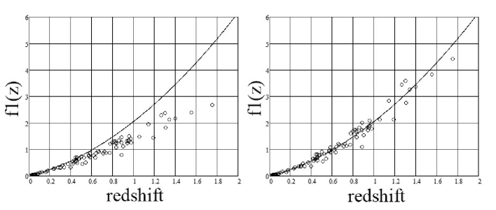
Figure 1: The theoretical function $f_{1}(z)$ of this model with $b=2.137$ (solid); Supernovae 1a observational data from Table 5 of [10] transformed to the linear scale (circles, 82 points): corrected for time dilation (left panel) and corrected for no time dilation (right panel).

I describe here some features of a non-geometrical approach to quantum gravity [3] which leads to another interplay of gravitation and cosmology. My model is based on the idea of an existence of the background of super-strong interacting gravitons. An interaction of light with this background gives a specific redshift mechanism which does not need any cosmological expansion; its peculiarity is an additional relaxation of any light flux that may be connected with the observed deviation of the Hubble diagram from its expected view without dark energy in the standard model. Due to this relaxation, any observer can see only a part of the universe; the property is sufficient to explain the very important results of observations of a bulk flow of clusters reported in [1] without any exotic and dark names. In the model, the Newton and Hubble constants may be computed. An important feature of the model is an essential difference of inertial and gravitational masses of black holes; it means that an existence of black holes contradicts to the equivalence principle. Additionally, the property of asymptotic freedom of this model at very short distances leads to the important consequence: a black hole mass threshold should exist [4, 5]. A full mass of black hole should be restricted from the bottom with $m_{0}$; the rough estimate for it is: $m_{0}\sim 10^{7}M_{\odot}$. The range of transition to gravitational asymptotic freedom for a pair of protons is between $10^{-11}-10^{-13}$ meter, while for a pair of electrons it is between $10^{-13}-10^{-15}$ meter. This transition is non-universal [4]; it means that a geometrical description of gravity on this or smaller scales, for

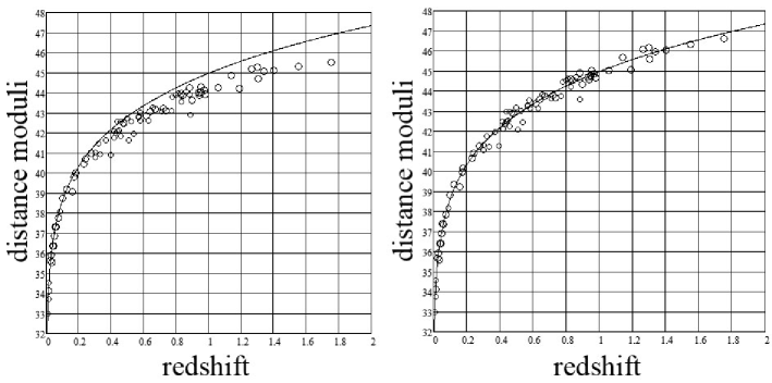
Figure 2: The theoretical Hubble diagram $\mu_{0}(z)$ of this model with $b=2.137$ (solid); Supernovae 1a observational data from Table 5 of [10] (circles, 82 points): corrected for time dilation (left panel) and corrected for no time dilation (right panel).

example on the Planck one, is not valid. Theoretical predictions for galaxy/quasar number counts were found in this model [6] based only on the luminosity distance and the geometrical one as functions of a redshift; there is not any visible contradiction with observations.

In the model, the luminosity distance $D_{L}$ is equal to [3]:

$$D_{L}=a^{-1}\ln(1+z)\cdot(1+z)^{(1+b)/2}\equiv a^{-1}f_{1}(z),$$

where $f_{1}(z)\equiv\ln(1+z)\cdot(1+z)^{(1+b)/2}$, $a=H/c,$ and $b=2.137$ for soft radiation. Time dilation is absent in this model; but observational data are usually corrected for this effect of the standard cosmological model [7, 8]. Due to the correction for time dilation, the observed flux is overestimated in $(1+z)$ times, and one should correct distance moduli $\mu_{0}=5\log D_{L}+25$ as [9]:

$$\mu_{0}^{{}^{\prime}}=\mu_{0}+2.5\log(1+z),$$

where $\mu_{0}^{{}^{\prime}}$ are distance moduli in any model without time dilation. The comparison of predictions of the model with Supernovae 1a observational data by Riess et al. [10] is shown on Figs. 1, 2. On Fig. 1, I have used the linear scale of the vertical axis; to re-compute values of $f_{1}(z)$ from observations, one can apply the transformation:

$$f_{1}(z)=10^{(\mu_{0}(z)-c_{1})/5},$$

where $c_{1}$ is a constant (here its value is $c_{1}=43.4$). The left panels of

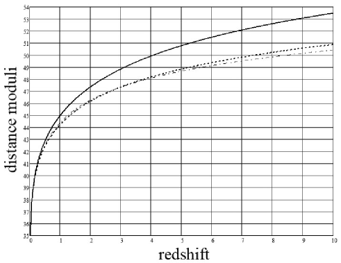
Figure 3: The three theoretical Hubble diagrams: $\mu_{0}(z)$ of this model with $b=2.137$ (solid); $\mu_{0}(z)$ of this model with $b=1.137$ taking into account the effect of time dilation of the standard model (dash); $\mu_{c}(z)$ for a flat Universe with the concordance cosmology by $\Omega_{M}=0.27$ and $w=-1$ (dadot).

these figures are the same as Figs. 2, 3 of [3]; it is obvious now that the essential differences between predictions of the model and observations were caused namely by the correction for cosmological time dilation. After the correction for no time dilation, the same observations are fitted very well with the theoretical curve (the right panels). Some further details may be found in my recent paper [11].

As it was shown in [12], theoretical distance moduli $\mu_{c}(z)$ for a flat Universe with the concordance cosmology by $\Omega_{M}=0.27$ and $w=-1$, which give the best fit to GRB observations by Schaefer [13], are very close to the Hubble diagram $\mu_{0}(z)$ with $b=1.1$ of this model. From the considered above, we see that the avoidance of the effect of cosmological time dilation means the transition to $b=2.137-1=1.137$ - very close to that value. We may do now some predictions about the behavior of the universe in a frame of the standard model for high $z$ comparing the theoretical Hubble diagrams (see Fig. 3): $\mu_{0}(z)$ of this model with $b=1.137$ taking into account the effect of time dilation of the standard model (dash); and $\mu_{c}(z)$ for a flat Universe with the concordance cosmology by $\Omega_{M}=0.27$ and $w=-1$ (dadot). You can see a good accordance of this diagrams up to $z\approx 4;$ for higher redshifts we should expect the accelerated expansion again. The extra acceleration should decrease from big $z$ to the smaller ones. We must bide new data from the future space missions to verify this prediction.

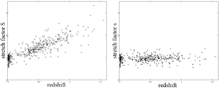
Figure 4: The observed values of stretch factor $S$ without correction for time dilation (left panel, $\times$) and the corresponding values of stretch factor $s$ corrected for time dilation (right panel, $+$); data are taken from Table 11 of [14] by Kowalski et al. (the Union compilation of SNe 1a).

Let us discuss briefly the distributions of stretch factor values of Supernovae 1a. Supernovae light curves are characterized by observers with the observed timescale stretch factor $S$. In the standard cosmological model, to find the stretch factor $s$ in the supernova rest frame one should divide $S$ by $(1+z)$, where the factor $(1+z)^{-1}$ takes into account the effect of time dilation [7]. After it, the timescale of light curve is corrected by the factor $S$, when its magnitude is corrected only by the stretch factor $s$ – in the standard model approach; but in any model with no time dilation it is necessary to use the factor $S$ for both normalizations. On Fig. 4, the data from the Union compilation of SNe 1a by Kowalski et al. [14] are used to show the distributions of values of $S$ and $s$ for nearby SNe 1a (104 points with $z\leq 0.1$) and for high-z SNe 1a (294 points with $z>0.1$). The values of the average $\langle s\rangle$ and $\sigma$ for $s$ are almost identical for these two subsamples: $\langle s\rangle$ is equal to $0.91$ and $0.97$, $\sigma$ is equal to $0.143$ and $0.144$ for nearby and remote events. Usually, it is interpreted as the main argument in the proof that time dilation takes place [7]. But there are obvious physical arguments to show that the distributions of the stretch factor should be different for nearby and remote explosions: $1)$ the lower boundary of the distribution should rise with $z$ due to increasing the luminosity distance; $2)$ the upper boundary should rise too because we have not a possibility to observe in the local volume very rare events, and they may be seen only in a very big volume. We see both these expected peculiarities on the left panel of Fig. 4, but not on the right one.

In this model, energy losses of any massive body due to forehead collisions with gravitons lead to the body acceleration by a non-zero velocity $v$: $w_{0}=-ac^{2}(1-v^{2}/c^{2}).$ For small velocities: $w_{0}\simeq-Hc,$ that may be connected with the Pioneer anomaly [15].

Astrophysical and cosmological observations may be used not only as confirmations of the standard model from new and new dark sides but in another manner: to clarify and to found better our knowledge of gravitation, perhaps, even beyond general relativity.

References

- [1] Kashlinsky, A. et al. ApJ 2010, 712, L81-l85 [http://arxiv.org/abs/0910.4958].
- [2] Anderson, J.D. et al. Phys. Rev. Lett. 1998, 81, 2858; Phys. Rev. 2002, D65, 082004; [gr-qc/0104064 v4].
- [3] Ivanov, M.A. In the book ”Focus on Quantum Gravity Research”, Ed. D.C. Moore, Nova Science, NY - 2006 - pp. 89-120; [hep-th/0506189], [http://ivanovma.narod.ru/nova04.pdf].
- [4] Ivanov, M.A. [arXiv:0901.0510v1 [physics.gen-ph]].
- [5] Ivanov, M.A. Gravitational asymptotic freedom and matter filling of black holes. Contribution to PIRT-09, Moscow, 6-9 July 2009 [http://vixra.org/abs/0907.0036].
- [6] Ivanov, M.A. [astro-ph/0606223].
- [7] Perlmutter, S. et al. Bull. Am. Astron. Soc. 1997, 29, 1351 [astro-ph/9812473v1].
- [8] Blondin, S. et al. ApJ 2008, 682, 724-736 [arXiv:0804.3595v1].
- [9] Brynjolfsson, Ari [astro-ph/0406437v2].
- [10] Riess, A.G. et al. ApJ 2004, 607, 665; [astro-ph/0402512].
- [11] Ivanov, M.A. Contribution to the VI Int. Workshop on the Dark side of the Universe (DSU2010), Guanajuato U., Leon, Mexico, 1-6 June, 2010 [http://ivanovma.narod.ru/no-time-dilation10.pdf].
- [12] Ivanov, M.A. [astro-ph/0609518].
- [13] Schaefer, B.E. [astro-ph/0612285].
- [14] Kowalski, M. et al. ApJ 2008, 686, 749-778; [arXiv:0804.4142v1 [astro-ph]].
- [15] Ivanov, M.A. [arXiv:0711.0450v2 [physics.gen-ph]].