Acceleration techniques for regularized Newton methods applied to electromagnetic inverse medium scattering problems

Abstract

We study the construction and updating of spectral preconditioners for´ regularized Newton methods and their application to electromagnetic inverse medium scattering problems. Moreover, we show how a Lepskiĭ-type stopping rule can be implemented efficiently for these methods. In numerical examples, the proposed method compares favorably with other iterative regularization method in terms of work-precision diagrams for exact data. For data perturbed by random noise, the Lepskiĭ-type stopping rule performs considerably better than the commonly used discrepancy principle.

1 Introduction

In this paper we study the efficient numerical solution of an inverse scattering problem for time harmonic electromagnetic waves. The forward problem is essentially described by the time-harmonic Maxwell equations

$$\mbox{curl }\mbox{curl }\mathbf{E}(\mathbf{r})-\kappa^{2}n(\mathbf{r})^{2}\mathbf{E}(\mathbf{r})=0$$

for the electric field $\mathbf{E}$. Our aim is to reconstruct a local inhomogeneity of the refractive index $n$ of a medium, given far field measurements for many incident waves. A more detailed discussion of the forward problem is given in §2.

After discretization the inverse problem is described by a nonlinear, ill-conditioned system of equations ${\bf F}({\bf x})={\bf y}$ with a function ${\bf F}:D({\bf F})\subset\mathbb{R}^{M}\to\mathbb{R}^{N}$, which is infinitely smooth on the subset $D({\bf F})\subset\mathbb{R}^{M}$ where it is defined. Since the system is highly ill-conditioned, we have consider the effects of data noise. Here we assume an additive noise model for the observe data ${\bf y}^{\rm obs}$:

$${\bf y}^{\rm obs}={\bf F}({\bf x})+{\bf\epsilon}$$ (1)

The noise vector ${\bf\epsilon}$ is assumed to be a vector of random variables with known finite covariance matrix and a known bound on the expectation $\|\mathbb{E}{\bf\epsilon}\|\leq\delta$.

In this article we contribute to preconditioning techniques for the Levenberg-Marquardt algorithm and the iteratively regularized Gauss-Newton method (IRGNM). These methods are obtained by applying Tikhonov regularization with some an initial guess ${\bf b}_{k}$ and a regularization parameter $\gamma_{k}$ to the Newton equations ${\bf A}_{k}{\bf h}_{k}={\bf y}^{\rm obs}-{\bf F}({\bf x}_{k})$. Here ${\bf A}_{k}:={\bf F}^{\prime}[{\bf x}_{k}]\in\mathbb{R}^{N\times M}$ denotes the Jacobian of ${\bf F}$ at ${\bf x}_{k}$. This leads to normal equations of the form

$${\bf G}_{k}^{\top}{\bf G}_{k}{\bf h}_{k}={\bf G}_{k}^{\top}{\bf g}_{k}$$ (2)

with

$${\bf G}_{k}:=\left(\begin{array}[]{c}{\bf A}_{k}\\ \sqrt{\gamma_{k}}{\bf I}\end{array}\right)\in\mathbb{R}^{(N+M)\times M}\qquad\mbox{and}\qquad{\bf g}_{k}:=\left(\begin{array}[]{c}{\bf y}^{\rm obs}-{\bf F}({\bf x}_{k})\\ \sqrt{\gamma_{k}}{\bf b}_{k}\end{array}\right).$$

The choice ${\bf b}_{k}=0$ corresponds to the Levenberg-Marquardt algorithm and the choice ${\bf b}_{k}={\bf x}_{0}-{\bf x}_{k}$ to the IRGNM. As opposed to the Levenberg-Marquardt algorithm as used in optimization we simply choose the regularization parameter $\gamma_{k}$ of the form

$$\gamma_{k}=\gamma_{0}\gamma^{-k}\qquad\mbox{with }\gamma>1.$$ (3)

Convergence and convergence rates of the IRGNM in an infinite dimensional setting have been studied first in [2, 7, 19]. For further references and results including a convergence analysis of Levenberg-Marquardt algorithm we refer to the monographs [1, 22].

As an alternative, Hanke [17] suggested to apply the conjugate gradient (CG) method the normal equation ${\bf A}_{k}^{\top}{\bf A}_{k}{\bf h}_{k}={\bf A}_{k}^{\top}({\bf y}^{\rm obs}-{\bf F}({\bf x}_{k}))$ and use the regularizing properties of the CG method applied to the normal equation with early stopping. This is referred to as Newton-CG method. Regularized Newton methods with inner iterative regularization methods have also been studied by Rieder [31, 32]. Finally, applying a gradient method to the functional ${\bf x}\mapsto\frac{\mu}{2}\|{\bf F}({\bf x})-{\bf y}^{\rm obs}\|_{2}^{2}$ leads to the nonlinear Landweber iteration ${\bf x}_{k+1}:={\bf x}_{k}-\mu{\bf A}_{k}^{\top}({\bf F}({\bf x}_{k})-{\bf y}^{\rm obs})$ first studied in [18]. For an overview on iterative regularization methods for nonlinear ill-posed problems we refer to [22].

A continuation method for inverse electromagnetic medium scattering problems with multi-frequency data has been studied in [3]. For an overview on level set methods for inverse scattering problems we refer to [11, 12].

For the inverse electromagnetic scattering problem studied in this paper the evaluation of $\bf{F}$ and one row of its Jacobian $\bf{A}_{k}$ is very expensive and involves the solution of a three-dimensional forward scattering problem for many incident waves. Therefore, a computation of the full Jacobian is not reasonable, and regularization method for the inverse problem should only access $\bf{A}_{k}$ via matrix-vector multiplications ${\bf v}\mapsto{\bf A}_{k}{\bf v}$ and ${\bf g}\mapsto{\bf A}_{k}^{\top}{\bf g}$. Hence, from the methods discussed above only Landweber iteration and Newton-CG can be implemented directly. However, the convergence of Landweber iteration is known to be very slow, which is confirmed by our numerical experiments reported in §6. Preconditioning techniques for Landweber iteration have been studied in [13], but it is not clear how to apply these techniques to inverse electromagnetic medium scattering problems since the operator does not act in Hilbert scales. To use the IRGNM and Levenberg-Marquardt, we have to solve the system of equations (2) by iterative methods. It turns out that standard iterative solvers need many iterations since the systems becomes very ill-conditioned as $\gamma_{k}\to 0$.

For the efficient solution of these linear systems we apply the CG-method and exploit its close connection to Lanczos’ method. The latter method is used to approximately compute eigenpairs of ${\bf G}_{k}^{\top}{\bf G}_{k}$ to construct a spectral preconditioner for the CG-method. Since the eigenvalues $\lambda_{1}\geq\ldots\geq\lambda_{M}$ of ${\bf A}_{k}^{\top}{\bf A}_{k}$ decay at an exponential rate, it turns out that the approximations determined by Lanczos’ method are well suited to construct an efficient spectral preconditioner. Spectral preconditioning is reviewed in §3. In §4 we describe how the original method proposed in [20] can be improved by the construction of updates of the preconditioner during the Newton iteration. For a convergence analysis of the IRGNM in combination with the discrepancy principle (4) discussed below we refer to [24, 26]. It should be mentioned that all known convergence results need some condition restricting the degree of nonlinearity of ${\bf F}$, and unfortunately none of these conditions has been verified for the electromagnetic medium scattering problem.

An essential element of any iterative regularization method for an ill-posed problem is a data-driven choice of the stopping index. The most common rule is Morozov’s discrepancy principle [30], which consists in stopping the Newton iteration at the first index $K$ satisfying

$$\|{\bf F}({\bf x}_{K})-{\bf y}^{\rm obs}\|\leq\tau\delta<\|{\bf F}({\bf x}_{k})-{\bf y}^{\rm obs}\|,\qquad 0\leq k<{K},\quad\tau>1.$$ (4)

The discrepancy principle is also frequently used for random noise setting $\delta=\sqrt{\mathbb{E}\|{\bf\epsilon}\|^{2}}$. However, it is easy to see that this cannot give good results in the limit $N\to\infty$ (see e.g. [5]), and this is confirmed in our numerical experiments. In §5 we show how a Lepskiĭ-type stopping rule can be implemented efficiently in combination with the regularization method studied in §4.

Finally, in §6 we report on some numerical experiments to demonstrate the efficiency of the methods proposed in this paper.

2 electromagnetic medium scattering problem

The propagation of time-harmonic electromagnetic waves in an inhomogeneous, non-magnetic, isotropic medium without free charges is described by the time-harmonic Maxwell equations

$$\mbox{curl }\mbox{curl }\mathbf{E}(\mathbf{r})-\kappa^{2}(1-a(\mathbf{r}))\mathbf{E}(\mathbf{r})=0,\qquad\mathbf{r}\in\mathbb{R}^{3}$$ (5a)

(see [8]). Here $$\mathbf{E}:\mathbb{R}^{3}\to\mathbb{C}^{3} \Re\left(\mathbf{E}(\mathbf{r})e^{-i\omega t}\right) \omega>0 \kappa:=\sqrt{\varepsilon_{0}\mu_{0}}\omega \varepsilon_{0} \mu_{0}$$ describes the space-dependent part of a time-harmonic electromagnetic field of the form with angular frequency . Moreover, denotes the wave number, the electric permittivity of vacuum, and the magnetic permeability of vacuum. The refractive index of the medium given by

$$n(\mathbf{r})=\sqrt{1-a(\mathbf{r})}$$

is assumed to be $$C^{1,\alpha} \,\mathrm{supp}\,a\subset B_{1}=\{\mathbf{r}\in\mathbb{R}^{3}:|\mathbf{r}|<1\}$$-smooth, real and positive in this paper. Moreover, we assume that . Now, given a plane incident wave

$$\mathbf{E}^{\mathrm{i}}(\mathbf{r})=\mathbf{E}^{\mathrm{i}}(\mathbf{r};\mathbf{d},\mathbf{p})=\exp(-i\kappa\mathbf{r}\cdot\mathbf{d})\mathbf{p}$$

with direction $$\mathbf{d}\in S^{2} \mathbf{p}\in\mathbb{C}^{3} \mathbf{p}\cdot\mathbf{d}=0 \mathbf{E}:\mathbb{R}^{3}\to\mathbb{C}^{3} \mathbf{E}^{\mathrm{s}}:=\mathbf{E}-\mathbf{E}^{\mathrm{i}}$$ and polarization such that , the forward scattering problem consists in finding a total field satisfying (5a) such that the scattered field satisfies the Silver-Müller radiation condition

$$\lim_{|\mathbf{r}|\to\infty}\left(\mbox{curl }\mathbf{E}^{\mathrm{s}}(\mathbf{r})\times\mathbf{r}-i\kappa|\mathbf{r}|\mathbf{E}^{\mathrm{s}}(\mathbf{r})\right)=0$$ (5b)

uniformly for all directions $\hat{\mathbf{r}}=\mathbf{r}/|\mathbf{r}|\in S^{2}$. The latter condition implies that $\mathbf{E}^{\mathrm{s}}$ has the asymptotic behavior

$$\mathbf{E}^{\mathrm{s}}(\mathbf{r};\mathbf{d},\mathbf{p})=\frac{e^{i\kappa|\mathbf{r}|}}{|\mathbf{r}|}\mathbf{E}^{\infty}(\hat{\mathbf{r}};\mathbf{d},\mathbf{p})+O\left(\frac{1}{|\mathbf{r}|^{2}}\right),\qquad|\mathbf{r}|\to\infty$$

with a function $\mathbf{E}^{\infty}(\cdot;\mathbf{d},\mathbf{p}):S^{2}\to\mathbb{C}^{3}$ called the far field pattern of $\mathbf{E}^{\mathrm{s}}$. It satisfies $\mathbf{E}^{\infty}(\hat{\mathbf{r}};\mathbf{d},\mathbf{p})\cdot\hat{\mathbf{r}}=0$.

The inverse problem studied in this paper is to reconstruct $a$ given measurements of $\mathbf{E}^{\infty}(\hat{\mathbf{r}};\mathbf{d},\mathbf{p})$ for all $\hat{\mathbf{r}},\mathbf{d}\in S^{2}$ and $\mathbf{p}\in\mathbb{C}^{3}$ such that $\mathbf{d}\cdot\mathbf{p}=0$.

The forward scattering problem has an equivalent formulation in terms of the electromagnetic Lippmann-Schwinger equation

$$\mathbf{E}(\mathbf{r})+\kappa^{2}\int_{B_{1}}\!\!\Phi(\mathbf{r}-\tilde{\mathbf{r}})a(\tilde{\mathbf{r}})\mathbf{E}(\tilde{\mathbf{r}})\,{\rm d}\tilde{\mathbf{r}}+\mbox{grad }\!\!\int_{B_{1}}\!\!\Phi(\mathbf{r}-\tilde{\mathbf{r}})\frac{\mbox{grad }a(\tilde{\mathbf{r}})}{1-a(\tilde{\mathbf{r}})}\cdot\mathbf{E}(\tilde{\mathbf{r}})\,{\rm d}\tilde{\mathbf{r}}=\mathbf{E}^{i}(\mathbf{r})$$ (6)

for $\mathbf{r}\in\mathbb{R}^{3}$ with the scalar fundamental solution $\Phi(\mathbf{r}):=\exp(i\kappa|\mathbf{r}|)/(4\pi|\mathbf{r}|)$. For the numerical solution of the forward scattering problems we use a fast solver of (6), which converges super-linearly for smooth refractive indices (see [21]).

We typically use between $3\cdot 32^{3}=98304$ and $3\cdot 64^{3}=786\,432$ degrees of freedom to represent $\mathbf{E}(\cdot;\mathbf{d},\mathbf{p})$ for each $\mathbf{d},\mathbf{p}\in S^{2}$. The unknown perturbation $a$ of the refractive index is represented by a set of coefficients $\mathbf{x}\in\mathbb{R}^{M}$ with $500\leq M\leq 2\,000$ using tensor products of splines in radial direction and spherical harmonics in angular direction (see [20]). Moreover, we use 25 incident waves with random incident directions $\mathbf{d}_{j}$ and random polarizations $\mathbf{p}_{j}$ where the directions $\mathbf{d}_{j}$ were drawn from the uniform distribution on $S^{2}$. The exact data are given by complex numbers $\mathbf{E}^{\infty}(-\tilde{\mathbf{d}}_{l};\mathbf{d}_{j},\mathbf{p}_{j})\cdot\tilde{\mathbf{p}}_{l}$ for $j\in\{1,\dots,25\}$ and $l\in\{1,\dots,100\}$ where the $\tilde{\mathbf{d}}_{j}$ and $\tilde{\mathbf{p}}_{j}$ were generated in the same way as the $\mathbf{d}_{j}$ and $\mathbf{p}_{j}$. This yields a real data vector $\mathbf{y}\in\mathbb{R}^{N}$ of size $N=2\cdot 25\cdot 100=5000$.

3 spectral preconditioning

3.1 CG method and Lanczos’ method

Let us start by recalling the preconditioned conjugate gradient (CG) method and its connection to Lanczos’ method (see e.g. [10, 15, 33]). We consider a preconditioned equation

$${\bf M}^{-1}{\bf G}^{\top}{\bf G}{\bf h}={\bf M}^{-1}{\bf G}^{\top}{\bf g},$$ (7)

where ${\bf G}\in\mathbb{R}^{N\times M}$ is an arbitrary matrix of rank $M$, and ${\bf M}\in\mathbb{R}^{M\times M}$ is a symmetric and positive definite preconditioning matrix. Although the matrix ${\bf M}^{-1}{\bf G}^{\top}{\bf G}$ is not symmetric in general, the induced linear mapping in $\mathbb{R}^{M}$ is symmetric and positive definite with respect to the scalar product $\left<x,y\right>_{{\bf M}}:=\left<{\bf M}x,y\right>$ since

$$\left<{\bf M}^{-1}{\bf G}^{\top}{\bf G}{\bf x},{\bf y}\right>_{{\bf M}} = \left<{\bf x},{\bf G}^{\top}{\bf G}{\bf y}\right>=\left<{\bf x},{\bf M}^{-1}{\bf G}^{\top}{\bf G}{\bf y}\right>_{{\bf M}},$$

$$\left<{\bf M}^{-1}{\bf G}^{\top}{\bf G}{\bf x},{\bf x}\right>_{{\bf M}} = \left<{\bf x},{\bf G}^{\top}{\bf G}{\bf x}\right>=\|{\bf G}{\bf x}\|^{2}>0\quad\mbox{for }{\bf x}\neq 0.$$

Therefore, the CG-method applied to (7) can be coded as follows:

Algorithm 1

(Preconditioned conjugate gradient method)

• ${\bf h}^{0}=0;\hskip 2.84544pt{\bf d}^{0}={\bf g};\hskip 2.84544pt{\bf r}^{0}={\bf G}^{\top}{\bf d}^{0};\hskip 2.84544pt{\bf p}^{1}={\bf z}^{0}={\bf M}^{-1}{\bf r}^{0};\hskip 2.84544ptl=0;$

• while $\|{\bf r}^{l}\|>\varepsilon\gamma\|{\bf h}^{l}\|$

  • $l=l+1;$

  • ${\bf q}^{l}={\bf G}{\bf p}^{l};$

  • $\alpha_{l}=\left<{\bf r}^{l-1},{\bf z}^{l-1}\right>/\|{\bf q}^{l}\|^{2};$

  • ${\bf h}^{l}={\bf h}^{l-1}+\alpha_{l}{\bf p}^{l};$

  • ${\bf d}^{l}={\bf d}^{l-1}-\alpha_{l}{\bf q}^{l};$

  • ${\bf r}^{l}={\bf G}^{\top}{\bf d}^{l};$

  • ${\bf z}^{l}={\bf M}^{-1}{\bf r}^{l};$

  • $\beta_{l}=\left<{\bf r}^{l},{\bf z}^{l}\right>/\left<{\bf r}^{l-1},{\bf z}^{l-1}\right>;$

  • ${\bf p}^{l+1}={\bf z}^{l}+\beta_{l}{\bf p}^{l}$.

The stopping criterion $\|{\bf r}^{l}\|>\varepsilon\gamma\|{\bf h}^{l}\|$ ensures a relative accuracy of $\varepsilon/(1-\varepsilon)$ of the approximate solution if $\|((\bf{G}^{\top}\bf{G})^{-1}\|\leq 1/\gamma$ (i.e. $\gamma=\gamma_{k}$ if ${\bf G}={\bf G}_{k}$, see [24, 25]).

Quantities arising in Algorithm 1 can be used to approximate the largest eigenvalues and corresponding eigenvectors of ${\bf M}^{-1}{\bf G}^{\top}{\bf G}$ as follows: Multiplying ${\bf z}^{j}={\bf p}^{j+1}-\beta{\bf p}^{j}$ from the left by $\|{\bf z}^{j}\|^{-1}_{{\bf M}}{\bf G}$ and using the definitions and identities

$$\tilde{{\bf z}}^{j}:=\frac{{\bf z}^{j}}{\sqrt{({\bf z}^{j})^{\top}{\bf M}{\bf z}^{j}}},\quad\tilde{{\bf q}}^{j}:=\frac{{\bf q}^{j}}{\|{\bf q}^{j}\|},\qquad\frac{\|{\bf q}^{j+1}\|}{\|{\bf z}^{j}\|_{{\bf M}}}=\frac{1}{\sqrt{\alpha_{j+1}}},\quad\frac{\|{\bf q}^{j}\|}{\|{\bf z}^{j}\|_{{\bf M}}}=\frac{1}{\sqrt{\alpha_{j}\beta_{j}}}$$

yields

$${\bf G}\tilde{{\bf z}}^{0}=\frac{1}{\sqrt{\alpha_{1}}}\tilde{{\bf q}}^{j},\quad{\bf G}\tilde{{\bf z}}^{j}=\frac{1}{\sqrt{\alpha_{j+1}}}\tilde{{\bf q}}^{j+1}-\sqrt{\frac{\beta_{j}}{\alpha_{j}}}\tilde{{\bf q}}^{j},\qquad j=1,\ldots,l-1.$$ (8)

The identity $\alpha_{j}{\bf q}^{j}={\bf d}^{j-1}-{\bf d}^{j}$ multiplied from the left by $(\|{\bf q}^{j}\|\alpha_{j})^{-1}{\bf G}^{\top}$ together with

$$\frac{\|{\bf z}^{j-1}\|_{{\bf M}}}{\|{\bf q}^{j}\|\alpha_{j}}=\frac{1}{\sqrt{\alpha_{j}}},\qquad\frac{\|{\bf z}^{j}\|_{{\bf M}}}{\|{\bf q}^{j}\|\alpha_{j}}=\sqrt{\frac{\beta_{j}}{\alpha_{j}}}$$

yields

$${\bf M}^{-1}{\bf G}^{\top}{\bf\tilde{q}}^{j}=\frac{1}{\sqrt{\alpha_{j}}}{\bf z}^{j-1}-\sqrt{\frac{\beta_{j}}{\alpha_{j}}}{\bf z}^{j},\qquad j=1,\ldots,l.$$ (9)

Putting (8) and (9) together we have for all $j=1,\ldots,l-1$

$${\bf M}^{-1}{\bf G}^{\top}{\bf G}\tilde{{\bf z}}^{0} = \frac{1}{\alpha_{1}}\tilde{{\bf z}}^{0}-\frac{\sqrt{\beta_{1}}}{\alpha_{1}}\tilde{{\bf z}}^{1},$$

$${\bf M}^{-1}{\bf G}^{\top}{\bf G}\tilde{{\bf z}}^{j} = -\frac{\sqrt{\beta_{j}}}{\alpha_{j}}\tilde{{\bf z}}^{j-1}+\left(\frac{1}{\alpha_{j+1}}+\frac{\beta_{j}}{\alpha_{j}}\right)\tilde{{\bf z}}^{j}-\frac{\sqrt{\beta_{j+1}}}{\alpha_{j+1}}\tilde{{\bf z}}^{j+1}.$$

These formulas can be rewritten as

$${\bf M}^{-1}{\bf G}^{\top}{\bf G}{\bf Z}_{l}={\bf Z}_{l}{\bf T}_{l}-\left(0,\ldots,0,\frac{\sqrt{\beta_{l}}}{\alpha_{l}}\tilde{{\bf z}}^{l}\right)$$ (10)

where ${\bf Z}_{l}:=(\tilde{{\bf z}}^{0},\ldots,\tilde{{\bf z}}^{l-1})$ and

$${\bf T}_{l}:=\left(\begin{array}[]{ccccc}\frac{1}{\alpha_{1}}&-\frac{\sqrt{\beta_{1}}}{\alpha_{1}}\\ -\frac{\sqrt{\beta_{1}}}{\alpha_{1}}&\frac{1}{\alpha_{2}}+\frac{\beta_{1}}{\alpha_{1}}&-\frac{\sqrt{\beta_{2}}}{\alpha_{2}}\\ &\ddots&\ddots&\ddots\\ &&\ddots&\ddots&-\frac{\sqrt{\beta_{l-1}}}{\alpha_{l-1}}\\ &&&-\frac{\sqrt{\beta_{l-1}}}{\alpha_{l-1}}&\frac{1}{\alpha_{l}}+\frac{\beta_{l-1}}{\alpha_{l-1}}.\end{array}\right),$$

If we denote by $\theta_{1}>\ldots>\theta_{l}>0$ and ${\bf v}_{1},\ldots,{\bf v}_{l}$ the eigenvalues with corresponding eigenvectors of the symmetric and positive definite matrix ${\bf T}_{l}$, (10) implies

$${\bf Z}_{l}^{\top}{\bf M}^{-1}{\bf G}^{\top}{\bf G}{\bf Z}_{l}{\bf v}_{j}=\theta_{j}{\bf v}_{j},\qquad j=1,\ldots,l.$$

Hence, in the case that ${\bf z}^{l}$ vanishes $\theta_{1}>\ldots>\theta_{l}$ are exact eigenvalues of ${\bf M}^{-1}{\bf G}^{\top}{\bf G}$ with corresponding eigenvectors ${\bf Z}_{l}{\bf v}_{1},\ldots,{\bf Z}_{l}{\bf v}_{l}$. In the typical case ${\bf z}^{l}\neq 0$ the vectors ${\bf Z}_{l}{\bf v}_{j}$ usually converge rapidly to the eigenvectors corresponding to the outliers in the spectrum of ${\bf M}^{-1}{\bf G}^{\top}{\bf G}$ (cf. [10, 15] and the references on the Kaniel-Paige theory therein) and Lanczos’ method can be interpreted as a particular case of the Rayleigh-Ritz method. This connection can be used to interpret the so-called Ritz values $\theta_{1}>\ldots>\theta_{l}$ and the Ritz vectors ${\bf Z}_{l}{\bf v}_{1},\ldots,{\bf Z}_{l}{\bf v}_{l}$ as approximations to some eigenpairs of ${\bf M}^{-1}{\bf G}^{\top}{\bf G}$.

If ${\bf W}{\bf\Lambda}{\bf W}^{\top}$ is an eigendecomposition of the matrix ${\bf T}_{l}$ with ${\bf M}={\bf I}$, i.e. ${\bf W}=({\bf w}_{1},\ldots,{\bf w}_{\tilde{l}})$ is orthogonal and ${\bf\Lambda}=\mbox{diag}(\theta_{1}^{(2)},\ldots,\theta_{\tilde{l}}^{(2)})$, one can prove the equality (see [24])

$$\|{\bf G}^{\top}{\bf G}({\bf Z}_{\tilde{l}}{\bf w}_{i})-({\bf Z}_{\tilde{l}}{\bf w}_{i})\theta_{i}^{(2)}\|=\frac{\sqrt{\beta_{\tilde{l}}}}{\alpha_{\tilde{l}}}|{\bf w}_{i}(\tilde{l})|,\qquad i=1,\ldots,\tilde{l},$$ (11)

where ${\bf w}_{i}(\tilde{l})$ denotes the bottom entry of ${\bf w}_{i}$. This identity can be used to judge the accuracy of the Ritz pairs and to decide which of them to use in the spectral preconditioner.

3.2 Spectral preconditioning with Tikhonov regularization

Assume now that ${\bf G}$ is of the special form

$${\bf G}:=\left(\begin{array}[]{c}{\bf A}\\ \sqrt{\gamma}\;{\bf I}\end{array}\right)$$

with ${\bf A}\in\mathbb{R}^{N\times M}$. Let ${\bf u}_{1},\dots,{\bf u}_{M}$ be orthonormal eigenvectors of ${\bf A}^{\top}{\bf A}$, and let $\lambda_{1},\dots,\lambda_{M}$ be the corresponding eigenvalues.

Given eigenpairs $(\lambda_{j},{\bf u}_{j})$ for $j$ in some non-empty subset $\mathcal{J}\subset\{1,2,\dots,M\}$, we define a spectral preconditioner for ${\bf G}^{\top}{\bf G}=\gamma{\bf I}+{\bf A}^{\top}{\bf A}$ by

$${\bf M}:=\gamma{\bf I}+\sum_{j\in\mathcal{J}}\lambda_{j}{\bf u}_{j}({\bf u}_{j})^{\top}.$$

Its properties are summarized in the following proposition:

Proposition 2

Assume that $\mathrm{rank}(\mathbf{A})=M$. Then

• ${\bf M}$ is symmetric and positive definite, and its inverse is given by

  $${\bf M}^{-1}=\frac{1}{\gamma}{\bf I}+\sum_{j\in\mathcal{J}}\left(\frac{1}{\lambda_{j}+\gamma}-\frac{1}{\gamma}\right){\bf u}_{j}{\bf u}_{j}^{\top}.$$

• ${\bf M}^{-1}{\bf G}^{\top}{\bf G}{\bf x}={\bf x}+\sum_{j\notin\mathcal{J}}\frac{\lambda_{j}}{\gamma}\left<{\bf x},{\bf u}_{j}\right>{\bf u}_{j}={\bf G}^{\top}{\bf G}{\bf M}^{-1}{\bf x}$.

• The spectrum of the preconditioned matrix is given by

  $$\sigma({\bf M}^{-1}{\bf G}^{\top}{\bf G})=\left\{1+\frac{\lambda_{j}}{\gamma}:j\notin\mathcal{J}\right\}\cup\{1\},$$ (12)

  and the eigenvalue $1$ has multiplicity $\#\mathcal{J}$.

• If $\mu\neq 1$ is an eigenvalue of ${\bf M}^{-1}{\bf G}^{T}{\bf G}$ with corresponding eigenvector $\mathbf{u}$, then $(\gamma(\mu-1),\mathbf{u})$ is an eigenpair of $\mathbf{A}^{\top}\mathbf{A}$.

Proof: ${\bf M}$ is obviously symmetric, and it is positive definite since all its eigenvalues are $\geq\gamma>0$. The formula for the inverse follows from a straightforward computation.

Let $\mathcal{U}:=\mathrm{span}\{u_{j}:j\in\mathcal{J}\}$. Identifying matrices with their induced linear mappings, we have ${\bf M}|_{\mathcal{U}}={\bf G}^{\top}{\bf G}|_{\mathcal{U}}$ and ${\bf M}|_{\mathcal{U}^{\perp}}=\gamma{\bf I}|_{\mathcal{U}^{\perp}}$, and $\mathcal{U}$ and $\mathcal{U}^{\perp}$ are invariant under all the involved linear mappings. Therefore,

$${\bf M}^{-1}{\bf G}^{\top}{\bf G}|_{\mathcal{U}}={\bf I}|_{\mathcal{U}}={\bf G}^{\top}{\bf G}{\bf M}^{-1}|_{\mathcal{U}},$$

$${\bf M}^{-1}{\bf G}^{\top}{\bf G}|_{\mathcal{U}^{\perp}}=\frac{1}{\gamma}{\bf G}^{\top}{\bf G}|_{\mathcal{U}^{\perp}}={\bf G}^{\top}{\bf G}{\bf M}^{-1}|_{\mathcal{U}^{\perp}}.$$

Since ${\bf G}^{\top}{\bf G}{\bf x}=\sum_{j=1}^{M}(\gamma+\lambda_{j})\left<{\bf x},{\bf u}_{j}\right>{\bf u}_{j}$ for all ${\bf x}\in\mathbb{R}^{M}$, assertion b) follows. c) is obtained from b) by inserting the eigenvectors ${\bf u}_{j}$ into the formula.

If $(\mu,{\bf u})$ is an eigenpair of ${\bf M}^{-1}{\bf G}^{T}{\bf G}$ and $\mu\neq 1$, it follows that ${\bf u}\in\mathcal{U}^{\perp}$. Therefore, $\mu{\bf u}=\frac{1}{\gamma}{\bf G}^{T}{\bf G}{\bf u}={\bf u}+\frac{1}{\gamma}{\bf A}^{\top}{\bf A}{\bf u}$. This implies assertion d). $\Box$

Remark 3

We comment on the assumption $\mathrm{rank}(\mathbf{A})=M$ in Proposition 2. For the acoustic medium scattering problem injectivity of the continuous Fréchet derivative $F^{\prime}[{\bf x}]$ has been shown in [20, Prop. 2.2]. For the electromagnetic medium scattering problem uniqueness proofs for the nonlinear inverse problem (see [9, 16]) can be modified analogously to show injectivity of $F^{\prime}[{\bf x}]$. It is easy to see that this implies injectivity of ${\bf A}$ if ${\bf A}$ is a sufficiently accurate discrete approximation of $F^{\prime}[{\bf x}]$ on a finite dimensional subspace.

4 IRGNM with updated spectral preconditioners

Spectral preconditioning in Newton methods is particularly useful for exponentially ill-posed problems such as the electromagnetic inverse medium scattering problem. Typically, Lanczos’ method approximates outliers in the spectrum well, whereas eigenvalues in the bulk of the spectrum are harder to approximate. Frequently the more isolated an eigenvalue is, the better the approximation (see [23] and [10, Chapter 7]). For exponentially ill-conditioned problems the spectrum of ${\bf G}_{k,m}^{\top}{\bf G}_{k,m}$ consists of a small number of isolated eigenvalues and a large number of eigenvalues clustering at $\gamma_{k}$. If all the large isolated eigenvalues are found and computed accurately, spectral preconditioning reduces the condition number significantly.

Updating the preconditioner may be necessary for the following reasons:

• If the matrix ${\bf G}_{k,m}^{\top}{\bf G}_{k,m}$ has multiple isolated eigenvalues, the Lanczos’ method approximates at most one Ritz pair corresponding to this multiple eigenvalue.

• During Newton’s method the regularization parameter $\gamma_{k}$ tends to zero. Hence, if we keep the number of known eigenpairs for the construction of the preconditioner ${\bf M}_{k,m}$ fixed, the number of CG-steps will increase rapidly during our frozen Newton method (see [25]).

In the preconditioned Newton iteration we keep the Jacobian ${\bf A}_{m}={\bf F}^{\prime}({\bf x}_{m})$ frozen for several Newton steps and replace eq. (7) by

$${\bf M}_{k,m}^{-1}{\bf G}_{k,m}^{\top}{\bf G}_{k,m}{\bf h}={\bf M}_{k,m}^{-1}{\bf G}_{k,m}^{\top}{\bf g}_{k},$$ (13a)

where

$${\bf G}_{k,m}:=\left(\begin{array}[]{c}{\bf A}_{m}\\ \sqrt{\gamma_{k}}\;{\bf I}\end{array}\right)\qquad\mbox{and}\qquad{\bf g}_{k}:=\left(\begin{array}[]{c}{\bf y}^{\rm obs}-{\bf F}({\bf x}_{k})\\ \sqrt{\gamma_{k}}{\bf b}_{k}\end{array}\right).$$ (13b)

Moreover, given some eigenpairs $\{(\lambda_{j}^{(m)},{\bf u}_{j}^{(m)}):j\in\mathcal{J}\}$ of ${\bf A}_{m}^{\top}{\bf A}_{m}$ with orthonormal eigenvectors ${\bf u}_{j}^{(m)}$, the spectral preconditioner is defined by

$${\bf M}_{k,m}:=\gamma_{k}{\bf I}+\sum_{j\in\mathcal{J}}\lambda_{j}^{(m)}{\bf u}_{j}^{(m)}({\bf u}_{j}^{(m)})^{\top}.$$ (14)

A preconditioned semi-frozen Newton method with updates of the preconditioner can be coded as follows:

Algorithm 4

Input: initial guess ${\bf x}_{0}$, data ${\bf y}^{\delta}$, $\delta$ and/or $\mathbf{Cov}_{\epsilon}$ (see (1))

• $k:=0$; $m:=0$

• repeat

  • Evaluate ${\bf F}({\bf x}_{k})$ and define ${\bf G}_{k,m},{\bf g}_{k}$ by (13b);

  • if $\sqrt{k+1}\geq\sqrt{m+1}+1$

    • $m:=k$;

    • Solve ${\bf G}_{k,k}^{\top}{\bf G}_{k,k}{\bf h}_{k}={\bf G}_{k,k}^{\top}{\bf g}_{k}$ by CG-method;

    • Compute via Lanczos’ method orthonormal Ritz pairs $\{(\mu_{j}^{(m)},{\bf u}_{j}^{(m)}):j\in\tilde{\mathcal{J}}\}$ of ${\bf G}_{k,k}^{\top}{\bf G}_{k,k}$;

    • Select subset $\mathcal{J}\subset\tilde{\mathcal{J}}$ (see (11)) and set $\lambda_{j}^{(m)}:=\gamma_{k}(\mu_{j}^{(m)}-1)$ for $j\in\mathcal{J}$ (see Prop. 2);

  • else

    • Define ${\bf M}_{k,m}$ by (14);

    • if MustUpdate()           (see Remark 4 below!)

      • Solve ${\bf M}_{k,m}^{-1/2}{\bf G}_{k,m}^{\top}{\bf G}_{k,m}{\bf M}_{k,m}^{-1/2}{\bf\tilde{h}}_{k}={\bf M}_{k,m}^{-1/2}{\bf G}_{k,m}^{\top}{\bf g}_{k}$ by CG-method;

      • ${\bf h}_{k}:={\bf M}_{k,m}^{1/2}{\bf\tilde{h}}_{k}$;

      • Compute Ritz pairs $\{(\mu_{j}^{(m)},{\bf u}_{j}^{(m)}):j\in\tilde{\mathcal{J}}_{2}\}$ of ${\bf M}_{k,m}^{-1/2}{\bf G}_{k,m}^{\top}{\bf G}_{k,m}{\bf M}_{k,m}^{-1/2}$ using Lanczos’ method;

      • Select subset $\mathcal{J}_{2}\subset\tilde{\mathcal{J}}_{2}$ (see Remark 6) and set $\lambda_{j}^{(m)}:=\gamma_{k}(\mu_{j}^{(m)}-1)$ for $j\in\mathcal{J}_{2}$;

      • Set $\mathcal{J}:=\mathcal{J}\cup\mathcal{J}_{2}$ and reorthogonalize $\{{\bf u}_{j}^{(m)}:j\in\mathcal{J}\}$;

    • else

      • Solve ${\bf M}_{k,m}^{-1}{\bf G}_{k,m}^{\top}{\bf G}_{k,m}{\bf h}_{k}={\bf M}_{k,m}^{-1}{\bf G}_{k,m}^{\top}{\bf g}_{k}$ by CG-method;

    • end

  • end

  • ${\bf x}_{k+1}:={\bf x}_{k}+{\bf h}_{k}$; $k:=k+1$;

• until Stop()    (see §5)

• Select stopping index $K$ (see §5) and return ${\bf x}_{K}$;

We add some remarks on heuristics and implementation details for Algorithm 4:

1. Usually round-off errors cause loss of orthogonality in the residual vectors ${\bf z}^{j}$ computed in Algorithm 1. This loss of orthogonality is closely related to the convergence of the Ritz vectors (see [10, 24]). To sustain stability, Algorithm 1 was amended by a complete reorthogonalization scheme based on Householder transformations (see [15]).

2. The necessity of reorthogonalization is also our reason for preconditioning with ${\bf M}_{k,m}^{-1/2}$ from both sides instead of ${\bf M}_{k,m}^{-1}$ from the left when updating the preconditioner. In the latter case, reorthogonalization would have to be performed with respect to the inner product $\langle\cdot,\cdot\rangle_{{\bf M}_{k,m}}$, which is more complicated. Note that

   $${\bf M}_{k,m}^{-1/2}{\bf x} = \frac{1}{\sqrt{\gamma_{k}}}{\bf x}+\sum_{j\in\mathcal{J}}\left(\frac{1}{\sqrt{\gamma_{k}+\lambda_{j}}}-\frac{1}{\sqrt{\gamma_{k}}}\right)({\bf u}_{j}^{\top}{\bf x}){\bf u}_{j},$$

   $${\bf M}_{k,m}^{1/2}{\bf x} = \sqrt{\gamma_{k}}{\bf x}+\sum_{j\in\mathcal{J}}\left(\sqrt{\gamma_{k}+\lambda_{j}}-\sqrt{\gamma_{k}}\right)({\bf u}_{j}^{\top}{\bf x}){\bf u}_{j}.$$

3. Spectrally preconditioned linear systems react very sensitively to errors in the eigenelements (see [14, 24]). Hence, to ensure efficiency of the preconditioner it is necessary that the approximations of the Ritz pairs used in the construction of the preconditioner be of high accuracy. This is achieved by choosing $\varepsilon=10^{-9}$ in Algorithm 1 when updating or recomputing the preconditioner, whereas $\varepsilon=1/3$ is sufficient otherwise. Numerical experience shows that computation time invested into improved accuracy of the Ritz pairs pays off in the following Newton steps.

4. MustUpdate(): We update the preconditioner if the last update or recomputation is at least 4 Newton steps ago and the number of inner iterations in the previous Newton step is $>5$.

5. We found it useful not to perform a complete recomputation of the current preconditioner if it works well. Therefore, we amend the condition $\sqrt{k+1}\geq\sqrt{m+1}+1$ by the additional requirement that the number of inner iterations in the previous step be not too small, say $>8$. The condition $\sqrt{k+1}\geq\sqrt{m+1}+1$ is a generalization of the rule to recompute the preconditioner whenever $k+1$ is a square number, which was proposed in the original paper [20]. Under certain conditions it was shown in [25] to be optimal among all rules where $\sqrt{\cdot}$ is replaced by a function $x\mapsto x^{\mu}$ with $\mu\in(0,1]$.

6. For updating the preconditioner we only select Ritz values of ${\bf M}_{k,m}^{-1/2}{\bf G}_{k,m}^{\top}{\bf G}_{k,m}{\bf M}_{k,m}^{-1/2}$ which are sufficiently well separated from the cluster at $1$, say $\geq 1.1$. First, these eigenvalues are usually computed more accurately by Lanczos’ method, and second, they are more relevant for preconditioning.

7. In the initial phase when the updates ${\bf h}_{k}$ are large, keeping the Jacobian frozen is not efficient. Therefore, we use other methods in this phase, e.g. Newton-CG. In some cases globalization strategies will be necessary in this phase, although this was not the case in the examples reported below.

5 Implementation of a Lepskiĭ-type stopping rule

Lepskiĭ-type stopping rules for regularized Newton methods have been studied in [4, 5]. We refer to the original paper [27] on regression problems and to [29, 28] for a considerable simplification of the idea and its application to linear inverse problems. As opposed to the discrepancy principle, Lepskiĭ-type stopping rules yield order optimal rates of convergence for all smoothness classes up to the qualification of the underlying linear regularization method (in case of random noise typically only up to a logarithmic factor).

A crucial element of Lepskiĭ’s method are estimates of the propagated data noise error, and the performance depends essentially on the sharpness of these estimates. Let ${\bf R}_{k}:=({\bf G}_{k}^{\top}{\bf G}_{k})^{-1}{\bf A}_{k}$. If $\mathbf{\epsilon}\in\mathbb{R}^{N}$ is a deterministic noise vector, an estimate of the propagated data noise error is given by

$$\|{\bf R}_{k}\mathbf{\epsilon}\|\leq\|{\bf R}_{k}\|\,\|\mathbf{\epsilon}\|\leq\frac{1}{2\gamma_{k}}\|\mathbf{\epsilon}\|,$$ (15)

and these estimates are sharp if $(\gamma_{k},\mathbf{\epsilon})$ is an eigenpair of ${\bf A}_{k}{\bf A}_{k}^{\top}$. However, if $\mathbf{\epsilon}$ is a random vector with $\mathbb{E}\mathbf{\epsilon}=0$, finite second moments with covariance matrix ${\bf Cov}_{\mathbf{\epsilon}}=(\mathrm{Cov}(\epsilon_{i},\epsilon_{j}))_{i,j=1..N}$, the estimate (15) is usually very pessimistic, and we have

$$\sqrt{\mathbb{E}\|{\bf R}_{k}\mathbf{\epsilon}\|^{2}}=\sqrt{\mathrm{trace}({\bf R}_{k}^{\top}{\bf Cov}_{\mathbf{\epsilon}}{\bf R}_{k})}.$$ (16)

Denoting the right hand side of (15) or (16), respectively, by $\Phi(k)$, the Lepskiĭ stopping rule is defined by

$$K_{\rm bal}:=\min\{k\leq K_{\max}:\|{\bf x}_{k}-{\bf x}_{m}\|\leq\rho\Phi(m),m=k+1,\dots,K_{\max}\}$$ (17)

with a parameter $\rho>4$ and a maximal Newton step number $K_{\max}$. We choose $\rho=4.1$ in our numerical experiments and $K_{\max}:=\max\{k\in\mathbb{N}:\Phi(k)\leq R\}$ with a reasonable upper bound on the size of propagated data noise in the optimal reconstruction. $R$ may be an a-priori known bound $\|\bf{x}-\bf{x}_{0}\|$. However, it is advisable to choose a smaller value of $R$ to reduce the number of Newton iterations. The final results ${\bf x}_{K_{\rm bal}}$ do not depend critically on $R$.

The main computational challenge in the implementation of the stopping rule (17) for random noise is the efficient and accurate computation of $\Phi(k)$. One possibility is to generate $L$ independent copies $\mathbf{\epsilon}_{1},\dots,\mathbf{\epsilon}_{L}$ of the noise vector and use the approximation $\Phi(k)\approx(L^{-1}\sum_{l=1}^{L}\|{\bf R}_{k}\mathbf{\epsilon}_{l}\|^{2})^{1/2}$. However, this involves the iterative solution of $L+1$ instead of $1$ least squares system and leads to a tremendous increase of the computational cost.

With the methods described in the previous sections we can construct approximations ${\bf R}_{k}^{\rm app}:=\sum_{j\in\mathcal{J}_{m}}\frac{\sqrt{\lambda_{j}}}{\gamma_{k}+\lambda_{j}}{\bf u}_{j}{\bf w}_{j}^{\top}$ of ${\bf R}_{k}$, which allow cheap matrix-vector multiplications not involving evaluations of the forward mapping ${\bf F}$. This yields the approximation

$$\Phi(k)\approx\left(\frac{1}{L}\sum_{l=1}^{L}\|{\bf R}_{k}^{\rm app}\mathbf{\epsilon}_{l}\|^{2}\right)^{1/2}.$$ (18)

Here ${\bf w}_{j}:={\bf A}_{m}{\bf u}_{j}/\|{\bf A}_{m}{\bf u}_{j}\|$ denote the approximated left singular vectors of ${\bf A}_{m}$, which can be computed directly by an appropriately modified Lanczos method (see e.g. [15]). In the case of white noise, i.e. ${\bf Cov}_{\mathbf{\epsilon}}=\sigma^{2}{\bf I}_{N}$, the expected value of the right hand side is given by the simple expression

$$\Phi(k)\approx\sigma\left(\sum_{j=\mathcal{J}_{m}}\frac{\lambda_{j}}{(\gamma_{k}+\lambda_{j})^{2}}\right)^{1/2}.$$ (19)

Obviously, equality holds in (19) if $(\lambda_{j}^{2})_{j\in\mathcal{J}_{m}}$ is a complete set of eigenvalues of ${\bf A}_{m}^{\top}{\bf A}_{m}$ (with multiplicities). Under certain assumptions it has been shown in [6] in an infinite dimensional setting that the left hand side can be bounded by a small constant times the right hand side uniformly in $\gamma_{k}$ if $(\lambda_{j}^{2})_{j\in\mathcal{J}_{m}}$ contains all eigenvalues $\geq\gamma_{k}$. Our numerical results in section 6 indicate that this approximation is sufficiently accurate.

Figure 1: An exact refractive index and its reconstruction by the IRGNM with updated preconditioner at iteration 23. The plots show the cube $[-1,1]^{3}$, the wave number is $\kappa=1$.

6 Numerical results

As a test example we use the refractive index shown in Figure 1. For further information on the forward problem and its numerical solution we refer to §2 and [21].

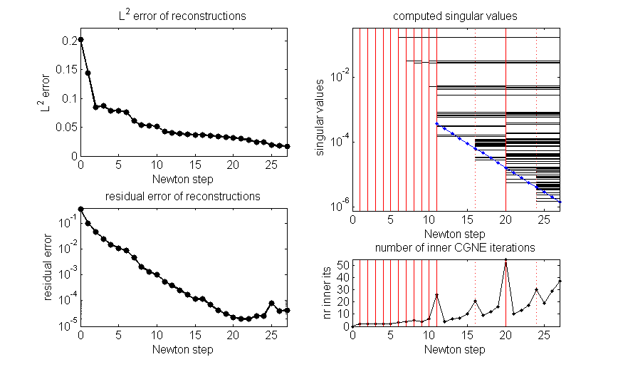
Figure 2: Performance of the preconditioned Newton method applied to the example in Figure 1. The left panels show the continuous $L^{2}$-error of the reconstructed refractive indices and the norm of the residuals $\|{\bf F}({\bf x}_{k})-{\bf y}^{\rm obs}\|_{2}$ over the Newton step $k$. The upper right panel shows the computed singular values used for preconditioning (solid horizontal lines). After step 11 the method changed from Newton-CG to IRGNM. At steps $m=11$ and $20$ the preconditioner was completely recomputed for the derivative at a new iterate. This is indicated by solid vertical lines. Updates of the preconditioner, indicated by dotted vertical lines, were performed at steps 16 and 24. The dots on the diagonal line indicate the values of the regularization parameter $\sqrt{\gamma_{k}}$. Some sufficiently accurate singular values computed during the Newton-CG phase are shown for their own interest although they were not used in the computation. The right lower panel shows the number of inner CGNE iterations over the Newton step $k$

Figure 2 illustrates the performance of the IRGNM with updated preconditioners. In the update steps for the preconditioner at $k=16$ and $24$ the new singular values mainly fall into two categories: First, we have singular values which are not well separated from the cluster for the regularization parameter $\gamma_{m}$ but are well separated for $\gamma_{k}$. These singular values are in or near the interval $[\sqrt{\gamma_{k}},\sqrt{\gamma_{m}}]$. The second category are multiple or nearly multiple singular values where only one element in the eigenspace is found in the application of Lanczos’ method. The use of an update clearly reduces the number of inner CGNE steps in the following Newton iterations.

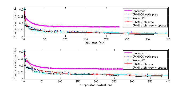
Figure 3: Work-precision diagram comparing the performance of different methods applied to the problem in Figure 1 for exact data.

Moreover, in Fig 3 we compared the speed of convergence of the iterative regularization methods discussed in the introduction for exact data. Here we measure ”speed” both in terms of cpu-time and in terms of the number of evaluations of ${\bf F}$, ${\bf F}^{\prime}[{\bf x}_{m}]$ or ${\bf F}^{\prime}[{\bf x}_{m}]^{\prime}$. Landweber iteration is clearly the slowest method although some good progress is achieved in the first few steps. The Newton-CG method performs very well up to some accuracy after which on it becomes slow, a behavior also observed in most other examples. We stopped the Newton-CG iteration at an $L^{2}$-error of $\approx 0.28$, which was achieved by the updated preconditioned IRGNM 2.5 times earlier. We also include a comparison with the preconditioned IRGNM without updating as suggested in [20]. The updating improves the performance particularly at high accuracies. Note that in the first Newton steps where $a$ is still small, the iterative solution of the forward problem is faster than in later Newton steps.

stopping rule	stopping index	$L^{2}$ error at stopping index
optimal	$15.93\pm 0.57$	$0.0406\pm 0.0010$
Lepskiĭ	$12.20\pm 0.54$	$0.0474\pm 0.0016$
discrepancy	$4.87\pm 0.43$	$0.0744\pm 0.0001$

Table 1: Performance of stopping rules averaged over 15 noise samples for the problem in Figure 1. The numbers indicate means and standard deviations.

Finally, we tested the performance of the Lepskiĭ-type stopping for randomly perturbed data. More precisely, we added independent Gaussian variables to each data point. The ”relative noise level” $\|\epsilon\|/\|{\bf y}\|$ was about $2\%$, but we stress that such a point-wise definition of the noise level does not make sense for random noise when considering the limit $N\to\infty$. We compare the discrepancy principle with $\tau=2$ to Lepskiĭ’s method with $\rho=4.1$. Moreover, we look at the optimal stopping index for each noise sample. As expected, the discrepancy principle stops the iteration too early. Note in Figure 2 that $\|{\bf F}({\bf x}_{k})-{\bf F}({\bf x})\|$ is at least an order of magnitude smaller than $\|\varepsilon\|$ at the optimal $k\approx 16$. (In Figure 2 we used exact data, but the behavior is similar for noisy data.) The results in Tab. 1 indicate that Lepskiĭ’s stopping rule is stable and yields considerably better results than the discrepancy principle.

Acknowledgments:

The second author acknowledges financial support by DFG (German Research Foundation) in the Research Training Group 1023 ”Identification in Mathematical Models: Synergy of Stochastic and Numerical Methods”.

References

• [1] A. Bakushinskii and M. Kokurin, Iterative methods for approximate solution of inverse problems, Springer, 2004.
• [2] A. B. Bakushinsky, The problem of the convergence of the iteratively regularized Gauss-Newton method, Comput. Maths. Math. Phys., 32 (1992), pp. 1353–1359.
• [3] G. Bao and P. Li, Inverse medium scattering problems for electromagnetic waves, SIAM J. Appl. Math., 65 (2005), pp. 2049–2066.
• [4] F. Bauer and T. Hohage, A Lepskij-type stopping rule for regularized Newton methods, Inverse Problems, 21 (2005), pp. 1975–1991.
• [5] F. Bauer, T. Hohage, and A. Munk, Regularized Newton methods for nonlinear inverse problems with random noise, SIAM J. Numer. Anal., 47 (2009).
• [6] N. Bissantz, T. Hohage, A. Munk, and F. Ruymgaart, Convergence rates of general regularization methods for statistical inverse problems and applications, SIAM J. Numer. Anal., 45 (2007), pp. 2610–2636.
• [7] B. Blaschke, A. Neubauer, and O. Scherzer, On convergence rates for the iteratively regularized Gauss-Newton method, IMA J. Num. Anal., 17 (1997), pp. 421–436.
• [8] D. Colton and R. Kress, Inverse Acoustic and Electromagnetic Scattering Theory, Springer, Berlin, Heidelberg, New York, second ed., 1997.
• [9] D. Colton and L. Päivärinta, The uniqueness of a solution to an inverse scattering problem for electromagnetic waves, Arch. Ration. Mech. Anal., 119 (1992), pp. 59–70.
• [10] J. Demmel, Applied Numerical Linear Algebra, Society for Industrial and Applied Mathematics, 1997.
• [11] O. Dorn and D. Lesselier, Level set methods for inverse scattering, Inverse Problems, 22 (2006), pp. R67–R131.
• [12]  , Level set methods for inverse scattering—some recent developments, Inverse Problems, 25 (2009), p. 125001.
• [13] H. Egger and A. Neubauer, Preconditioning Landweber iteration in Hilbert scales, Numer. Math., 101 (2005), pp. 643–662.
• [14] L. Giraud and S. Gratton, On the sensitivity of some spectral preconditioners, SIAM J. Matrix Anal. Appl., 27 (2006), pp. 1089–1105.
• [15] G. H. Golub and C. F. van Loan, Matrix Computations, The John Hopkins University Press, Baltimore, second ed., 1983.
• [16] P. Hähner, Stability of the inverse electromagnetic inhomogeneous medium problem, Inverse Problems, 16 (2000), pp. 155–174.
• [17] M. Hanke, Regularizing properties of a truncated Newton-CG algorithm for nonlinear inverse problems, Numer. Funct. Anal. Optim., 18 (1997), pp. 971–993.
• [18] M. Hanke, A. Neubauer, and O. Scherzer, A convergence analysis of the Landweber iteration for nonlinear ill-posed problems, Numer. Math., 72 (1995), pp. 21–37.
• [19] T. Hohage, Logarithmic convergence rates of the iteratively regularized Gauss-Newton method for an inverse potential and an inverse scattering problem, Inverse Problems, 13 (1997), pp. 1279–1299.
• [20]  , On the numerical solution of a three-dimensional inverse medium scattering problem, Inverse Problems, 17 (2001), pp. 1743–1763.
• [21]  , Fast numerical solution of the electromagnetic medium scattering problem and applications to the inverse problem, J. Comp. Phys., 214 (2006), pp. 224–238.
• [22] B. Kaltenbacher, A. Neubauer, and O. Scherzer, Iterative Regularization Methods for Nonlinear ill-posed Problems, Radon Series on Computational and Applied Mathematics, de Gruyter, Berlin, 2008.
• [23] A. Kuijlaars, Which eigenvalues are found by the Lanczos method?, SIAM J. Matrix Anal. Appl., 22 (2000), pp. 306–321.
• [24] S. Langer, Preconditioned Newton methods for ill-posed problems, PhD thesis, University of Göttingen, Germany, 2007.
• [25]  , Complexity analysis of the IRGNM with inner CG-iteration, J. Inv. Ill-Posed Probl., (to appear).
• [26] S. Langer and T. Hohage, Convergence analysis of an inexact iteratively regularized Gauss-newton method under general source conditions, Journal of Inverse and Ill-posed Problems, 15 (2007), pp. 311–327.
• [27] O. V. Lepskiĭ, On a problem of adaptive estimation in Gaussian white noise, Theory Probab. Appl., 35 (1990), pp. 454–466.
• [28] P. Mathé, The Lepskiĭ principle revisited, Inverse Problems, 22 (2006), pp. L11–L15.
• [29] P. Mathé and S. Pereverzev, Geometry of ill-posed problems in variable Hilbert scales, Inverse Problems, 19 (2003), pp. 789–803.
• [30] V. Morozov, On the solution of functional equations by the method of regularization, Soviet Math. Dokl., 7 (1966), pp. 414–417.
• [31] A. Rieder, On the regularization of nonlinear ill-posed problems via inexact Newton iterations, Inverse Problems, 15 (1999), pp. 309–327.
• [32] A. Rieder, Inexact Newton regularization using conjugate gradients as inner iteration, SIAM J. Numer. Anal., 43 (2005), pp. 604–622.
• [33] H. van der Vorst, Iterative Krylov Methods for Large Linear Systems, Cambridge University Press, Cambridge, 2003.