Elastic properties of graphene flakes: boundary effects and lattice vibrations

Abstract

We present a calculation of the free energy, the surface free energy and the elastic constants (“Lamé parameters” i.e, Poisson ratio, Young’s modulus) of graphene flakes on the level of the density functional theory employing different standard functionals. We observe that the Lamé parameters in small flakes can differ from the bulk values by 30% for hydrogenated zig-zag edges. The change results from the edge of the flake that compresses the interior. When including the vibrational zero point motion, we detect a decrease in the bending rigidity, $\kappa$, by $\sim 26\%$. This correction is depending on the flake size, $N$, because the vibrational frequencies flow with growing $N$ due to the release of the edge induced compression. We calculate Grüneisen parameters and find good agreement with previous authors.

I Introduction

Since its fabrication has become technologically feasibleNovoselov et al. (2004), graphene has been in the focus of frontier researchZhang et al. (2005); Novoselov et al. (2006); Geim and Novoselov (2007). One of its most celebrated properties are its massless low energy excitationsNovoselov et al. (2005); Castro Neto et al. (2009) (“Dirac fermions”), which emanate from the symmetries of the honeycomb lattice. The electronic properties of graphene flakes are quite different from bulk graphene due to the finite size and the presence of edgesNakada et al. (1996); Stampfer et al. (2009). In particular, calculations suggest that the zigzag edges of graphene nano-ribbons (quasi $1d$) have two flat bands at the Fermi energyFujita et al. (1996); Brey and Fertig (2006) that introduce magnetismWakabayashi et al. (1998); Son et al. (2006a, b); Hod et al. (2007a); jun Kan et al. (2008); Peres et al. (2006); Pisani et al. (2007); en Jiang et al. (2007). Recent theoretical studies on zigzag edged graphene flakes also confirm a tendency towards edge magnetismFernández-Rossier and Palacios (2007); Wang et al. (2009); Pisani et al. (2007); en Jiang et al. (2007). This gives additional motivation for fabricating graphene based nano structuresG mez-Navarro et al. (2008); Danneau et al. (2008); Lauffer et al. (2008); Li et al. (2008); Haluka et al. (2007); Miao et al. (2007) for further studies. The fabrication of such structures with well defined edges still poses a considerable technological challenge. Therefore, only very few experiments with structures exhibiting zigzag edges have been reportedCasiraghi et al. (2009); de Parga et al. (2008); Tan et al. (2009); a detailed investigation of the edge physics still needs to be done.

An increased interest in the elastic properties of graphene has developed recentlyFasolino et al. (2007); Gui et al. (2008); Atalaya et al. (2008); Garcia-Sanchez et al. (2008); G mez-Navarro et al. (2008); Lee et al. (2008); Pereira et al. (2009); Choi et al. (2010); Zakharchenko et al. (2009); Hod and Scuseria (2009); Cadelano et al. (2009); Guinea et al. (2009); Reddy et al. (2009); Lu et al. (2009); Ribeiro et al. (2009). This is, for instance, because experiments suggest that graphene samples exhibit a corrugated structureMeyer et al. (2007); Stolyarova et al. (2007); Ishigami et al. (2007); de Parga et al. (2008) (“ripples”) even at relatively low temperatures. Their origin is thought to be due to residual elastic strain produced by the experimental preparation techniqueBao et al. (2009).

Also for elastic properties, edge effects can be highly relevant. For this reason, flake elastic properties are certainly interesting in their own right. Namely, there is an intimate relation between the electronic structure and the atomic geometry of graphene. For example, the electronic spectrum of a certain class of arm-chair graphene nano-ribbons is reported to acquire a spectral gap due to an edge induced lattice dimerization along the transport directionSon et al. (2006b).

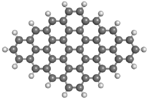
Figure 1: Geometry of the $N{\times}N$ hydrogenated graphene flakes(here $N{=}4$), that we have used for the density functional calculations.

In our study we investigate the free energy, the elastic properties, and the phonon spectrum of $N\times N$ graphene sheets (“flakes”) as displayed in Fig. 1 using the density functional theory (DFT). We show, that the different chemical nature of C-C bonds at the hydrogenated edge as compared to the bulk leads to an nearly homogenous compression, i.e. strain. As a consequence, the average C-C-distance in a $3\times 3$ flake is reduced by a substantial amount, $0.3\%$; for comparison, strain as achieved in typical pressure experiments does not usually exceed values $\sim 1\%$Mohiuddin et al. (2009); Lee et al. (2008); Chen et al. (2009).

The presence of the surface induced strain leaves various traces in the flakes’ interior observables. (a) The flakes elastic constants, i.e. the Lamé parameters, are enhanced as compared to the bulk case. For isotropic strain in smallest flakes ($3\times 3$), the (inverse) compressibility $\mu+\lambda$ (precise definition see below, Eq. (2)) increases by 30%; for shear forces the increase is even bigger, almost a factor of 2. (b) Under bond compression the interatomic forces typically increase, so that even the short wavelength vibrations, in particular the optical phonons, exhibit a “blue shift” of their frequencies with decreasing flake sizes. This flow can be seen in the variation of the Raman spectra with strain Ferrari et al. (2006); Ni et al. (2008); Casiraghi et al. (2009); Mohiuddin et al. (2009); Proctor et al. (2009); Tsoukleri et al. (2009) and can be described in the standard manner by Grüneisen parameters. The values that we find here of Grüneisen parameters, agree reasonably well with previous reportsMohiuddin et al. (2009); Reich et al. (2000); Ni et al. (2008).

Even though one might suspect, that our topics have already been dealt with extensively in the literatureSánchez-Portal et al. (1999); Reich et al. (2000, 2002); Hod et al. (2007b); Tsoukleri et al. (2009), a detailed investigation of the elastic properties of nano-flakes is yet to be done; this refers, in particular, to an analysis of edge and finite size effects of hydrogenated zig-zag flakes which we perform in this work.

II Free energy of homogenous, planar flakes

We consider the free energy of a graphene flake as depicted in Fig. 1 with a homogenous C-C-distance, $d$, as the sum of all its bond energies:

$$F_{N}(d)=N_{\rm i}\Psi(d)+N_{\rm e}\psi(d)+N_{\rm c}\psi^{\rm c}(d)+\frac{\phi^{\rm e}(d)}{N_{\rm e}}+\frac{\phi^{\rm i}(d)}{N_{\rm i}}$$ (1)

where $N_{\rm i}$ denotes the number of internal C-C-bonds with an associated binding energy $\Psi$, $N_{\rm e}$ denotes the number of edge located C-C-bonds with energy $\psi$ and $\psi^{\rm c}$ includes the corner contributions, where $N_{\rm c}$ is the number of bonds linking the corner atoms, $N_{\rm c}{=}6$ in Fig. 1. The binding energy per C-C-CH edge group is close to $2\psi$ but not identical to it. For instance, $\psi$ also includes corrections of internal bonds, that still “feel” the presence of the surface. Similarly, $N_{c}\psi^{\rm c}$ is approximating the binding energy of the corner groups (two HC-CH groups and two C-CH-C groups).

We mention, that the representation (1) is slightly simplified in the following sense. In general, the boundary (shape) of a given flake, e.g as depicted in Fig. 1, does not share the hexagonal symmetry of the honeycomb lattice. For this reason, in flakes with a fully relaxed atomic structure bond lengths and bond angles are not strictly all the same. Our DFT-calculations indicate, however, that such distortions, though clearly detectable, give only small corrections to those phenomenological parameters that we are mostly interested in.

The continuum theory of $2d$-membranes has been devised for an inhomogeneous flake with neighboring bonds exhibiting slowly (in space ) varying bond distances, $d({\bf r})$, and angles. In this formulation the elastic energy is represented by the functionalLandau and Lifshitz (1959),

$$E = \frac{\kappa}{2}\int_{\cal A}\!d^{2}{\bf r}(\nabla^{2}h)^{2}+\frac{\mu+\lambda}{2}\int_{\cal A}d^{2}{\bf r}\ (u_{xx}{+}u_{yy})^{2}$$ (2)

$$+\frac{\mu}{2}\int_{\cal A}\!d^{2}{\bf r}\ \left[4u_{xy}^{2}+(u_{xx}{-}u_{yy})^{2}\right].$$

The flake coordinates are given with respect to a planar reference state with area ${\cal A}$, that lives in the ${\bf r}{=}(x,y)$-plane; accordingly, the in plane coordinates constitute the displacement vector, ${\bf u}(x,y)$, that measures the translation of each membrane point $(x,y,z)$ with respect to the reference state. The out of plane distortions define the height field $h(x,y)$; for the planar case $h{=}0$. ${\bf u}$ and $h$ together constitute the strain tensor ($i,j=x,y$),

$$u_{ij}=\frac{1}{2}\left[\partial_{i}u_{j}+\partial_{j}u_{i}+\partial_{i}h\partial_{j}h+\sum_{k}\partial_{i}u_{k}\partial_{j}u_{k}\right].$$ (3)

It is clear that the form of $u_{ij}$ depicted in Eq. (3) is symmetric construction, with respect to the spatial derivatives of ${\bf u}$ ensure its invariance under in plane rotations by $90^{\circ}$ which correspond to ${\bf u}\propto(y,-x)$.

The total elastic energy (2) is a sum over contributions which resemble local oscillators in the membrane plane. The first term is proportionate to the curvature $\nabla^{2}h$ and introduces the bending rigidity $\kappa$. It describes the energy cost for bending the membrane without changing the bond lengths or in plane bond angles. The Lamé parameters, $\lambda$ and $\mu$, appearing in the second and third term of Eq. (2) describe the in plane rigidity.

For homogenous, planar membranes the elastic theory (2) may be considered as a continuum approximation to (1) which does not make explicit reference to boundary terms. Edges are accounted for only in the boundary conditions and (possibly) in a dependency of the Lamé parameters on the position with respect to the edge. Usually not included in (2) is the fact that this spatial dependency supports long range terms, $\sim 1/{\rm flakesize}$. They modify the Lamé parameters appearing in (2) even inside the flake’s interior.

Phenomenological parameters

Isotropic strain:

In order to illustrate the cooperative effect between surface and bulk, we consider an expansion of (1) in terms of the variable $\varepsilon{=}(d-d_{0})/d_{0}$; $\varepsilon$ quantifies the strain inside the flake. The bulk free energy per bond has an expansion,

$$\Psi = \Psi_{0}+\frac{1}{2}\Psi_{2}\ \varepsilon^{2}+\frac{1}{6}\Psi_{3}\ \varepsilon^{3}+\frac{1}{24}\Psi_{4}\ \varepsilon^{4}\ldots$$ (4)

where the bulk bond length $d_{0}$ is to be determined at $N_{{\rm i,e}}\to\infty$. The surface free energy may also be expanded about a minimum bond length, $d_{0}^{\rm e}$, but in general $d_{0}^{\rm e}\neq d_{0}$. After all, in the limit $N_{{\rm i,e}}\to\infty$, just the first term in Eq. (1) contributes to the free energy per area and therefore $d_{0}$ needs to minimizes $\Psi$, only. Hence, we introduce the relative deviation of surface and bulk optimal bond lengths, ${\mathfrak{d}}{=}(d_{0}-d_{0}^{\rm e})/d_{0}$, so that we have an expansion

$$\psi = \bar{\psi}_{0}+\frac{1}{2}\bar{\psi}_{2}\ (\varepsilon{+}{\mathfrak{d}})^{2}+\frac{1}{6}\bar{\psi}_{3}\ (\varepsilon{+}{\mathfrak{d}})^{3}+\frac{1}{24}\bar{\psi}_{4}\ (\varepsilon{+}{\mathfrak{d}})^{4}\ldots$$ (5)

$$\equiv \psi_{0}+\psi_{1}\ \varepsilon+\frac{1}{2}\psi_{2}\ \varepsilon^{2}+\frac{1}{6}\psi_{3}\ \varepsilon^{3}+\ldots$$

where the coefficients in the second line are defined in terms of the expansion the line before. The elastic properties of the flake are determined by the expansion parameters $\Psi_{2,3,4},\psi_{1,2,3}$.

At any finite value of $N_{{\rm i,e}}$, optimization must also include the boundary (i.e. surface) terms and therefore the optimal value of $\varepsilon$, $\varepsilon_{N}$, is non-vanishing in this case; specifically,

$$\varepsilon_{N} = -\frac{\psi_{1}}{\Psi_{2}}\frac{N_{\rm e}}{N_{\rm i}}$$

$$\approx -{\mathfrak{d}}\ \frac{\bar{\psi}_{2}}{\Psi_{2}}\frac{N_{\rm e}}{N_{\rm i}}.$$

In order to calculate the feedback of this shift into the elastic parameters, we expand $F$ in the vicinity of its minimum, $\varepsilon_{N}$, to the fourth order in $\varepsilon$. Recalling that this corresponds to a strain ${\bf u}({\bf x}){=}\varepsilon{\bf x}$ we can compare the result with Eq. (2) and thus find:

$$\mu+\lambda=\frac{1}{4}\left(\Psi_{2}+\frac{N_{\rm e}}{N_{\rm i}}\psi_{2}\right)+\frac{1}{4}\Psi_{3}\varepsilon_{N}$$

$$+\frac{\varepsilon}{12}\left(\Psi_{3}+\frac{N_{\rm e}}{N_{\rm i}}\psi_{3}+\Psi_{4}\varepsilon_{N}\right).$$ (7)

The first term in the rhs-expression (II) simply accounts for the separate, additive contributions of bulk and surface (i.e. edge) free energies. The edge contribution, that appears here, could formally be accounted for in a generalized version of Eq. (2) where one adds a boundary term. Similarly, by allowing for a dependency of the Lamé parameters on strain itself, one could also include additive an-harmonic effects, second bracket first two terms. In either case, the phenomenological parameters are universal in the sense, that they are the same for each flake size and geometry.

The interesting pieces are the terms in $\varepsilon_{N}$, which are mixing surface and bulk parameters: $\Psi_{3}\varepsilon_{N}\sim\psi_{1}\Psi_{3}/\Psi_{2}$. They encode the “cooperative” effect between boundary induced strain and bulk anharmonicities. It is due to them, that the flakes elastic parameters need to be adjusted in principle for every geometry separately.

Shear strain:

An analogous analysis as for the isotropic strain also applies to shear forces. The expansion is even in the shear strain ${\bf u}=(0,\varepsilon_{\rm s}x)$:

$$\Psi = \Psi_{0}+\frac{1}{2}\tilde{\Psi}_{2}\ \varepsilon_{\rm s}^{2}+\frac{1}{24}\tilde{\Psi}_{4}\ \varepsilon_{\rm s}^{4}+\ldots$$ (8)

$$\psi = \psi_{0}+\frac{1}{2}\tilde{\psi}_{2}\ \varepsilon_{\rm s}^{2}+\frac{1}{24}\tilde{\psi}_{4}\ \varepsilon_{\rm s}^{4}+\ldots.$$ (9)

The new expansion parameters, $\tilde{\Psi}_{i},\tilde{\psi}_{i},i=2,4,\ldots$, are, in general, dependent on the flake geometry. Again, by comparing to Eq. (2) we find

$$\mu=\tilde{\Psi}_{2}+\tilde{\psi}_{2}+\frac{1}{12}\varepsilon_{\rm s}^{2}\left(\tilde{\Psi}_{4}+\tilde{\psi}_{4}\right).$$ (10)

Here, surface and bulk free energies give strictly additive contributions, and a cooperative effect does not emerge.

III Density functional calculations

III.1 Method

In Fig. 1 we display the geometry of the $N\times N$-graphene flake that is employed in our calculations: $N_{\rm i}=(N-1)(3N-1)$, $N_{\rm e}=8(N-1)$. Electronic structure calculations have been performed for a given atomic configuration (C-C distance, flake geometry etc.) on the basis of the density functional theory as implemented in the quantum chemistry package TURBOMOLEAhlrichs et al. (1989). We are comparing GGA functionals (BP86Becke (1988); Perdew (1986), PBEPerdew and Wang (1992); Perdew et al. (1996)) with a hybrid functional (B3LYP Becke (1993)) and use a minimal basis set (SVPSchäfer et al. (1992)). Specifically, we are working at zero temperature and approximate the free (i. e. ground state) energy, Eq. (1), by the DFT estimate for the total binding energy of the flake:

$$F_{\rm el}(N,d):=E_{\rm el}(N,d)-E_{\rm free}(N).$$ (11)

with,

$$E_{\rm free}(N)=N_{\rm H}E_{\rm H}+N_{\rm C}E_{\rm C}$$ (12)

where $E_{\rm H/C}$ denote the DFT energies of a free charge neutral hydrogen/carbon atom and $N_{\rm H/C}$ denotes the number of hydrogen/carbon atoms in the flake.

III.2 Results and Discussion

Isotropic strain:

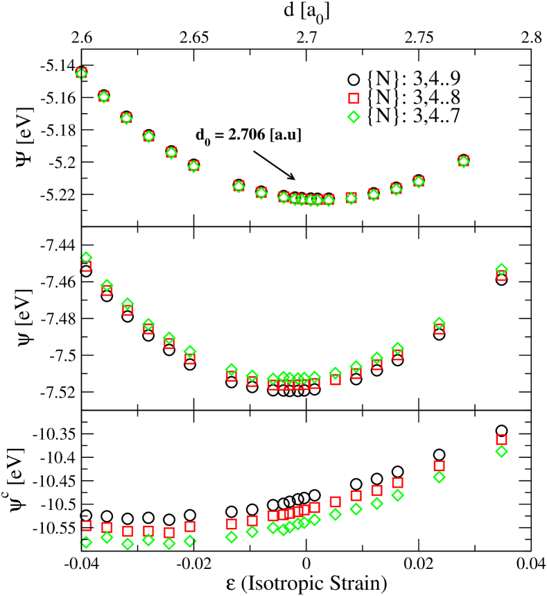
Figure 2: Bulk ($\Psi$), surface (edge, $\psi$) and corner ($\psi^{\rm c}$) free energy per carbon bond in the graphene flakes, Fig. 1, calculated with density functional theory (BP86-functional). Data based on the evaluation of three sets of flake sizes ranging from $\{N\}{=}3\ldots 9$, and a 5 parameter fit to Eqs. (1,11) per $d$ values. ($a_{0}$:= 0.529 $\AA$.)

A sequence of DFT calculations has been performed for $N{=}3\ldots 9$ and different values of the C-C distance, $d$. For each distance, $F_{\rm el}(N,d)$ has been calculated. In order to extract the expansion coefficients of Eq. (1), $\Psi(d),\psi(d),\psi^{\rm c}(d),\phi^{\rm e}(d),\phi^{\rm i}(d)$, we have performed five parameter fits on sets of raw DFT data. These fits were applied to three data sets consisting of $\{N\}{=}3,\ldots 7$, $\{N\}{=}3\ldots 8$ and $\{N\}{=}3\ldots 9$. The results for the surface, bulk and corner free energy have been displayed in Fig. 2. The scatter between the fitting parameters belonging to different data sets is relatively small, which illustrates the stability of the fit.

The lattice constant of bulk graphene is estimated from the minimum position of $\Psi(d)$ Fig. 2, upper panel as $d_{0}{=}2.706a_{0}$, where $a_{0}{=}0.529\AA$ denotes the Bohr radius. Comparing this position to the minimum of the edge (surface) free energy, Fig. 2, center panel, $d_{0}^{\rm e}{=}2.694a_{0}$, we find ${\mathfrak{d}}{=}0.44$%. This indicates clearly the compression of the C-C bond length near the edge. The shift of the minimum position to lower values becomes even more pronounced near the corners, i.e. in $\psi^{\rm c}(d)$, see Fig. 2, lower panel.

Furthermore, we can perform a certain consistency check by evaluating the bond energies. We have a binding energy $\Psi(d_{0}){=}-5.22$eV for bulk carbon atoms. The binding energy of $H$-atoms near edges (C-C-CH group) is approximately $\Delta E^{\rm e}_{\rm H}{\approx}2\psi(d_{0}){-}2\Psi(d_{0}){\approx}-4.6$eV; when going to the corners (HC-CH and C-CH-C groups) we have $\Delta E^{\rm c}_{\rm H}{\approx}\psi^{\rm c}(d_{0}){-}\Psi(d_{0})\approx-5.3$ which is roughly consistent with $\Delta E^{\rm e}_{\rm H}$, as it should be.

	$d_{0}[\AA]$	$d_{0}^{\rm e}[\AA]$
BP86	$1.432^{\pm 0.002}$	$1.427^{\pm 0.001}$
B3LYP	$1.426^{\pm 0.001}$	$1.421^{\pm 0.002}$
PBE	$1.431^{\pm 0.001}$	$1.426^{\pm 0.005}$

Table 1: Minimum C-C bond length as extracted from bulk free energy and surface free energy correspondingly (see Fig. 2, upper and middle panel). The distance in $d_{0}$ and $d_{o}^{\rm e}$ leads to a nearly homogenous pressure on the flake that modifies elastic and electronic-structure properties. Data is shown for three different functional used in DFT calculation.

To obtain also the other phenomenological parameters, a second (polynomial) fit of the traces $\Psi(d),\psi(d)$, Fig. 2, according to Eqs. (4,5) has been performed; all fitting parameters are summarized in Tab. 1,2 and 3.

	$-\Psi_{0}$ [eV]	$\frac{1}{2}\Psi_{2}$ [eV]	$-\frac{1}{6}\Psi_{3}$ [eV]
BP86	$5.223^{\pm 0.001}$	$46.301^{\pm 0.082}$	$128.301^{\pm 1.915}$
B3LYP	$5.008^{\pm 0.001}$	$47.723^{\pm 0.362}$	$154.59^{\pm 31.446}$
PBE	$5.373^{\pm 0.004}$	$45.57^{\pm 0.43}$	$187.309^{\pm 24.448}$

Table 2: Bulk free energy coefficients as defined in Eq. (4). These coefficients are extracted from fitting Eq. (4) to the data in Fig. 2, upper panel.

	$-\psi_{0}$  [eV]	$\psi_{1}$ [eV]	$\frac{1}{2}\psi_{2}$ [eV]	$-\frac{1}{6}\psi_{3}$ [eV]
BP86	$7.515^{\pm 0.006}$	$0.285^{\pm 0.015}$	$44.93^{\pm 0.43}$	$112.745^{\pm 18.718}$
B3LYP	$7.187^{\pm 0.006}$	$0.261^{\pm 0.015}$	$45.586^{\pm 2.154}$	$-$
PBE	$7.63^{\pm 0.01}$	$0.308^{\pm 0.011}$	$47.503^{\pm 1.082}$	$-$

Table 3: Edge (surface) coefficients as defined in Eq. (5). These coefficients are extracted from fitting Eq. (5) to the data in Fig. 2, middle panel.

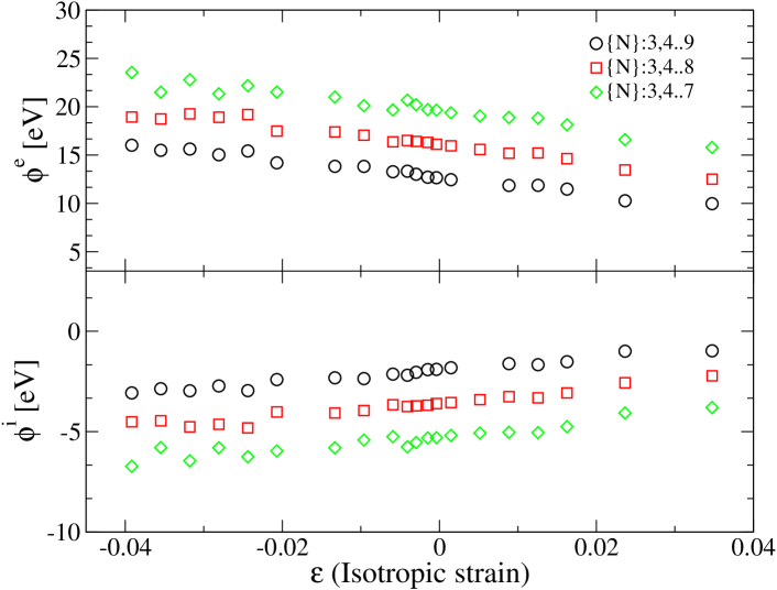
Figure 3: Dependency of the amplitudes $\phi^{\rm i,e}$ describing the corrections in $1/N_{\rm e,i}$ to the binding energy $\Delta F_{\rm el}(N)$. Data were obtained by the 5 parameters fit, already underlying the traces shown in Fig. 2.

When fitting the raw data to get $\Psi,\psi,\psi^{\rm c}$ the terms in $1/N_{\rm i,e}$ could not be neglected for the system sizes, that we considered. The corresponding amplitudes are displayed in Fig. 3. Unlike it was the case with the previous data, Fig. 2, the amplitudes $\phi^{\rm i,e}$ of the $1/N_{\rm i,e}$-corrections still exhibit a considerable variation with increasing system size, which is probably due to even higher order terms that have been neglected in the expansion Eq. (1). Interestingly, while the magnitude of $\phi^{\rm i,e}(\varepsilon)$ is still shifting the slope and perhaps also the sign of the two functions has converged, already. Under this assumption we may conclude, that both amplitudes flow closer to zero values when $\varepsilon$ increases. This behavior is compatible with the simple expectation, that the main effect incorporated in the $1/N_{\rm i,e}$-corrections is the discreteness of the flake’s electronic spectrum with level spacings $\Delta_{\rm i,e}$ for bulk and surface modes. With increasing $\varepsilon$ the bandwidth decreases and so do $\Delta_{\rm i,e}$ and $\phi^{\rm i,e}$.

Shear strain:

A largely analogous method as was adopted for the isotropic strain, has also been applied for shear forces. In this case, the convergence of the DFT calculations turned out to be considerably more difficult, so that the investigated system sizes range from $\{N\}{=}3\dots 7$, only. From our fitting procedure we could determine the response of the bulk and surface energy to the shear strain, $\varepsilon_{\rm s}$, as shown in Fig. 4. The parameters entering Eqs. (8,9) can be extracted and are listed in Tab. 4.

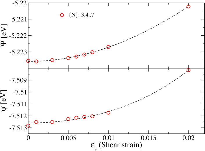
Figure 4: Change in the free energy when applying a shear strain in graphene flakes. Upper panel shows the change in bulk free energy per interior C-C bond; lower panel exhibits change in surface (edge) free energy per C-C bond. Data sets are for system sizes {N}=3$\ldots$7 and extracted from an expression analogous for shear to Eqs. (1,11). The lines indicate the polynomial fit according to Eqs. (8,9) with parameter given in Tab. 4.

[eV]	$\frac{1}{2}\tilde{\Psi}_{2}$	$-\frac{1}{24}\tilde{\Psi}_{4}$	$\frac{1}{2}\tilde{\psi}_{2}$	$\frac{1}{24}\tilde{\psi}_{4}$
BP86	8.396±0.426	871±50%	8.99±3.29	$5237^{\pm 60\%}$

Table 4: Bulk and surface shear free energy coefficients as extracted from fitting Eq. (8) (Eq. (9)) to the data in Fig. 4 upper panel (lower panel).

IV Flake elastic properties

In the previous subsection, the focus was on the behavior of the free energy on the flake size under isotropic and shear strain. In this section, we discuss and illustrate what our previous findings imply for the elastic properties of a single flake with a fixed size, $N$. Partly, we are considering the same set of data again, but now plotting observables directly for $N$ fixed.

IV.0.1 Homogenous isotropic strain

Fig. 5 shows, how the excess energy per unit cell grows under increasing strain for different flake sizes $N$. It is readily seen from this plot, that there is a shift of the equilibrium lattice constant $d(N)$ to smaller values. In the light of the previous section, this shift is the expected consequence of the surface induced strain $\varepsilon_{N}$. The inset shows, the scaling with $N_{\rm e}/N_{\rm i}$.

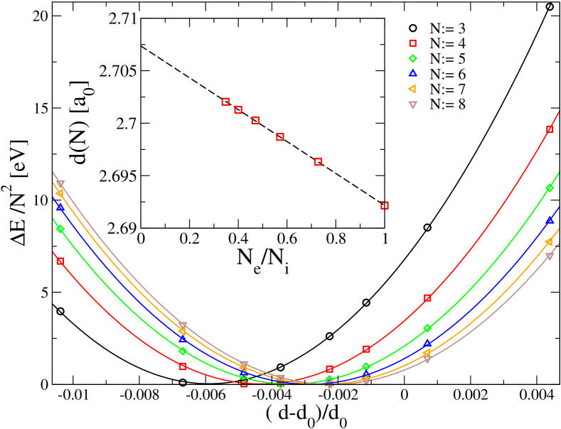
Figure 5: Excess energy $\Delta E$ per unit cell generated by rescaling all bond length, $d$, (homogeneous, isotropic strain). $\Delta E$ exhibits flow of the equilibrium bond length with the linear flake size $N$. Main panel: $\Delta E$ over bond length $d$ employed in the simulation. $d$ is measured relative to the bulk bond length. The lines serve as a guide to the eyes. Inset: Extrapolating the equilibrium bond length $d({N})$ into the bulk limit: $d_{\rm 0}=2.707\pm 0.001$.

In addition, we also extract the flake elastic constant $\mu{+}\lambda$ from the parabolic shape of the curves, Fig. 5. To this end, we replot the data in Fig. 6 left, so as to highlight the curvature and its strain dependency. On the basis of Eq. (II) we can conclude, that the offset of the curves is a consequence of (a) the presence of the surface and the extra energy required for its compression (term $N_{\rm e}/N_{\rm i}$ in Eq. (II)) and (b) the feedback of the surface strain $\varepsilon_{N}$ into the bulk C-C distance. Extrapolating the zero strain values into the limit, $N{\to}\infty$, we recover the previously derived bulk limit value. This check is displayed in Fig. 6, right. The plot also reveals, that the deviation of elastic parameters from their bulk values in small flakes may not be very small. For our smallest flakes, $N{=}3$ it reaches almost 30%.

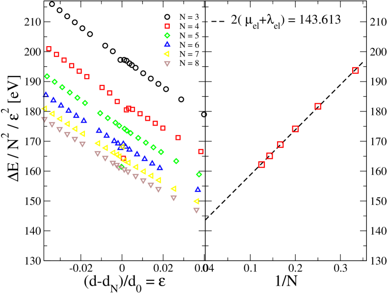
Figure 6: Estimating the sum of the Lamé parameters $\mu_{\rm el}+\lambda_{\rm el}$ and the boundary correction (offset of traces) from $\Delta E$ displayed in the previous Fig. 5. Left: Data for curvature exhibit a slope which indicates the linear dependency of the Lamé parameter $\lambda_{\rm{el}}$ on strain. (Linear terms in $\mu_{\rm{el}}$ do not appear, see Fig. 9.) Right: extrapolating the curvature at $\varepsilon=0$ into the bulk limit.

Additional information can be extracted from Fig. 6 left, about anharmonicities which manifest themselves in the slope of the curves displayed. This pre-factor of the an-harmonic term (linear in $\varepsilon$) in Eq. (II) admits the following interpretation. The slope changes with increasing $N$ since the contributions of the surface ($\psi_{3}$-term) and the surface induced bulk compression ($\Psi_{4}\varepsilon_{N}$-term) diminish. A non-vanishing value of $\Psi_{3}/12$ for the slope will remain however even in the bulk limit.

IV.0.2 Shear strain

Following the same strategy as we did before with Fig. 6, we plot in Fig. 7 the excess energy $\Delta E_{\rm s}$ induced by pure shear strain, ${\bf u}({\bf x})=\varepsilon_{\rm s}(0,x)$. Again, the plot emphasizes the curvature in this quantity, $\mu$, and how it evolves with the flake size.

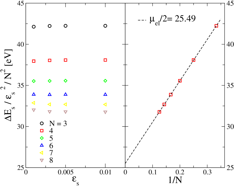
Figure 7: Estimate for Lamé parameter $\mu_{\rm el}$ determined from the excess energy $\Delta E_{\rm{s}}$ per unit cell under pure shear strain with strength $\varepsilon_{\rm s}$. (Procedure similar to previous Fig. 6.) Left panel: dependency of curvature of $\Delta E_{\rm{s}}(\varepsilon_{\rm{s}})$ on the linear flake size $N$. Due to mirror symmetries of the unit cell, linear corrections do not appear for the shear parameter $\mu_{\rm{el}}$. Right: extrapolating the curvature into the bulk limit.

Since $\Delta E_{\rm s}$ is even in the shear strain, only positive values of $\varepsilon_{\rm s}$ are given. Also, for the same reason an-harmonic terms exist only in the quartic order, so that the displayed data traces have zero slope. Similar to the previous case of isotropic strain, we also witness here a very strong dependency of the elastic constant on the flake size. In fact, for shear strain it reaches almost 70% for the small system sizes that we are considering.

	$d_{0}[\AA]$	$\mu_{\rm{el}}+\lambda_{\rm{el}}$[eV]	$\mu_{\rm{el}}$[eV]	$\nu$	Y[N$/$m]
BP86	1.432±0.001	70.715±0.011	50.95±0.01	0.162	356.23
B3LYP	1.427±0.001	71.21±0.12	-	-	-
PBE	1.431±0.002	69.027±0.012	-	-	-
prev.	1.42[Zakharchenko et al., 2009; Mounet and Marzari, 2005]	66.571[Zakharchenko et al., 2009]	49.45[Zakharchenko et al., 2009]	0.149[Kudin et al., 2001],	346[Zakharchenko et al., 2009]
calc.	1.41[Ribeiro et al., 2009]			0.173[Gui et al., 2008]	307[Reddy et al., 2009]
	1.45[Arroyo and Belytschko, 2004]			0.16[Arroyo and Belytschko, 2004]	345[Kudin et al., 2001]
				0.31[Cadelano et al., 2009]	336[Arroyo and Belytschko, 2004]
					312[Cadelano et al., 2009]
expt.	-	-	-	-	342[Lee et al., 2008]
(Graphene)
expt.	1.421[Weast and Astle, 2009]	-	-	0.165[Blakslee et al., 1970]	371[Bosak et al., 2007]
(Graphite)	1.422[Bosak et al., 2007]

Table 5: Comparison of C-C-bond distance in bulk graphene, elastic constants , Poisson ratio($\nu$) and Young’s modulus(Y) as extracted from Fig. (5,6,7) respectively by extrapolating the values in bulk limit ($N\rightarrow\infty$) with previous works. Data is shown for three different functionals we used in DFT calculation.

IV.0.3 Buckling induced strain

We present results from an additional DFT study, where we investigate the transverse stiffness of the graphene flake that gives rise to the elastic parameter $\kappa$. To this end we employ the following strategy. Each flake has a center pair or center ring of carbon atoms, see Figs. (1,8). To create a transverse probing field $h({\bf r})$, we lift the center atoms by the distance $h_{0}$ over the reference plane. After this, the atomic structure of the flake is relaxed under the constraint, that the set of edge atoms (H-atoms and edge C-atoms) can move only within the reference plane; edge atoms cannot shift in $h$-direction. In this way, a flake is equipped with a single ripple while at the same time the associated strain field ${\bf u}({\bf x})$ remains negligibly small. In order to estimate the integrated curvature we numerically compute the bi-variate function which interpolates the scattered data values($h({\bf r})$-field) at any predefined smooth mesh. We then use this interpolated function to perform the second order numerical derivative at any arbitrary precision.

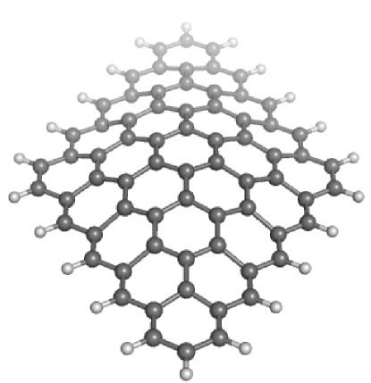
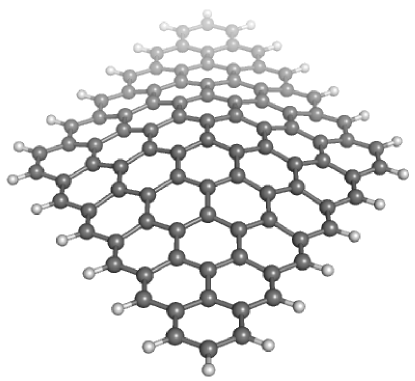
Figure 8: Buckling flakes of $N$=5, 6 with different central configurations of carbon atoms. The atomic configuration of C atoms is relaxed under the constraint that the center atoms remain at a given height $h_{0}$ above the ground plane, while edge atoms (H and C) remain sitting within this plane ($h=0$).

Fig. 9 displays how the excess energy $\Delta E_{h}$ associated with the ripple grows with the increased integrated curvature,

$$I_{\kappa}=\frac{1}{2}\int\ d^{2}{\bf r}\ (\Delta h({\bf r}))^{2}$$ (13)

The increase is linear, as expected from Eq. (2) with a slope that is only weakly dependent on the flake size, see inset Fig. 9, this implies that nonlinearities remain small as long as the ratio of the ripples amplitude and wave length , $h_{0}/L$, does not exceed $\sim$ 5%. The bending rigidity thus found is $\kappa_{\rm{el}}$ = 1.24 eV which is well consistent with the value 1.1eV obtained by Fasolino, Los and KatsnelsonFasolino et al. (2007).

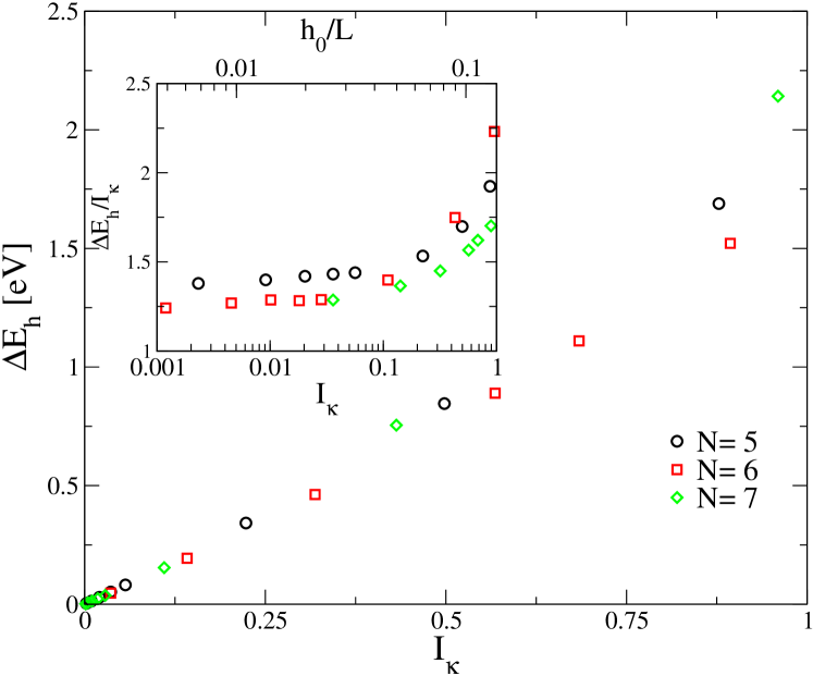
Figure 9: Estimating the Lamé parameter $\kappa$ determined from the excess energy $\Delta E$ of a bulging flake with maximum height at $h_{0}$ over the unperturbed (flat) plane (see Fig. 8). Main panel: Change of energy $\Delta E$ with the integrated curvature $I_{\kappa}=\int d^{2}{\bf r}\ (\Delta h({\bf r}))^{2}$ for different flake sizes $N$. Inset: The ratio $\kappa=\Delta E/I_{\kappa}$ depend on $N$ due to the effect of edge compression.

Notice, that there is a significant scattering of almost 20% in earlier theoretical estimates for $\kappa$ and derived quantities, see Tab. 2 in Ref. Odegard et al., 2002. Discrepancies appear because different theoretical techniques are being employed, e.g. empirical potentialsLu et al. (2009) and density functional theory, but also because of modeling artefacts. For example, extracting $\kappa$ from the elastic energy of carbon nano-tubes (radius $R$) requires a very careful extrapolation in $1/R$. If sub-leading terms are ignored, there is a pronounced tendency to overestimation, e.g. $\kappa=1.46$ eV in Ref. Kudin et al., 2001. These authors used nano-tubes with smaller tube radius, hence bigger curvature, where nonlinear effects become important. We can check the bending rigidity using the same curvature in Fig. 9 (inset) as reported in Ref. Kudin et al., 2001 and find a reasonable agreement with their value.

V Zero point motion

In this chapter we extend our analysis of flake elastic properties and take also the zero point motion of the atom cores into account, that constitute the hexagonal lattice. Now, the free energy acquires a second term,

$$F(N,d)=F_{\rm el}(N,d)+F_{\rm vib}(N,d)$$ (14)

with

$$F_{\rm vib}=\frac{1}{2}\sum_{p}\hbar\omega_{p}(N,d)$$ (15)

where $p$ labels all the flake’s vibrational modes. The vibrational excess energy associated with stretching the flake reads

$$\Delta F_{\rm vib}=\frac{\hbar}{2}\sum_{p}\omega_{p}(N,d)-\omega_{p}(N,d(N))$$ (16)

where $\omega(N,d(N))$ denotes the vibration energies in the absence of strain and $d(N)$ the equilibrium bond length, see inset Fig. 5. Also $\Delta F_{\rm vib}$ can be expanded in terms of the slow elastic modes,

$$\Delta F_{\rm{vib}}[h,{\bf u}]=\frac{1}{2}\int_{{\cal A}}d^{2}{\bf r}\,\gamma_{h}\left(\Delta h({\bf r})\right)^{2}-\int_{{\cal A}}d^{2}{\bf r}\,\sum_{ij}\gamma_{u}^{ij}u_{ij}({\bf r}),$$ (17)

with expansion parameters $\gamma_{h},\gamma_{u}$ that represent averages of Grüneisen parameters over all vibrational modes. In a two-dimensional sample with a mirror symmetry one expects $\gamma_{u}^{xy}=\gamma_{u}^{yx}=0$; the change in phonon frequencies should be even in the shear strain, $\varepsilon_{\rm s}$. Combining Eq. (17) with an expansion of $\Delta F_{\rm el}$ in full analogy with Eq. (2) and after completing the square, we find,

$$\Delta F_{\rm el\ vib}(N,d)=\frac{\kappa_{\rm el}+\gamma_{h}}{2}\ \int_{\it A}d^{2}{\bf r}(\nabla^{2}h)^{2}+\frac{\mu_{\rm el}+\lambda_{\rm el}}{2}\int_{A}d^{2}{\bf r}\left(u_{ii}-\frac{\gamma_{u}^{ii}}{\mu_{\rm el}+\lambda_{\rm el}}\right)^{2}+\frac{\mu_{\rm el}}{2}\int_{A}d^{2}{\bf r}\left(u_{xx}-u_{yy}\right)^{2}+u_{xy}^{2}.$$ (18)

For clarity, we have indicated in this expression the bare electronic coefficients (i.e. with frozen atomic cores) by $\kappa_{\rm el},\mu_{\rm el},\lambda_{\rm el}$. Likewise, the displacement field ${\bf u}({\bf x})$ is defined with respect to the optimum flake geometry ignoring vibrational terms.

In this way we can observe two facts. (i) Vibrations modify the bare transverse stiffness $\kappa_{\rm el}$ in Eq. (18), $\kappa=\kappa_{\rm{el}}+\gamma_{h}$. (ii) Vibrations also affect interatomic distances. The effect can be understood as an effective strain, which stretches the bare C-C distances: $\gamma_{u}^{ii}/(\mu_{\rm el}+\lambda_{\rm el})$. (iii) The change in the C-C bond lengths eventually feeds back into all elastic coefficients. Therefore, in a more complete treatment of higher order terms also modifications in $\mu_{\rm el},\lambda_{\rm el}$ would occur.

V.1 DFT calculations of the Grüneisen parameters

In order to estimate the Grüneisen parameters, $\gamma_{h},\gamma_{u}$, we should calculate the vibrational spectrum of flakes with and without applied strain. To this end we adopt the following procedure. For every flake size, $N$, we find the atomic geometry with the optimal electronic energy, see e.g. Fig. 1. This constitutes the set of freely relaxed “parent states”. The relaxation ensures the Hessian, that characterizes interatomic forces, to become a positive definite matrix.

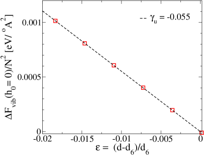
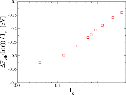
Figure 10: Left: Dependency of $\Delta F_{vib}$ on isotropic strain for system size $N{=}6$. The slope defines $\gamma_{u}$ as in Eq. (17). Right: Dependency of $\Delta F_{vib}$ on integrated curvature, $I_{\kappa}{=}\int\ d^{2}{\bf r}\ (\Delta h({\bf r}))^{2}$, as in Fig. 9.

In the present study we focus on the impact of phonons on the bulk elastic constants. There we may eliminate contributions of surface vibrations by assigning an infinite mass to the surface H and C atoms. Other than this, the calculation of vibrational modes and frequencies for the relaxed flake is a standard procedureDeglmann et al. (2002); Deglmann and Furche (2002).

Thereafter, each parent state thus obtained is used in order to create two new families. The first family is constructed to obtain $\gamma_{u}$. It derives by changing the bond length of edge C-C-pairs by a factor of $1+\varepsilon$ keeping all atoms still inside the base plane ($h{=}0$). For each value $\varepsilon$ the internal C-atoms are relaxed and the vibrational spectrum together with the average strain field, $I_{u}(\varepsilon)=\int d{\bf r}(u_{xx}{+}u_{yy})$, are recalculated. In this process it is important to have edge atoms at infinite mass. This ensures that the flake energy is in a (constrained) minimum so that all frequencies are real.

In order to determine $\gamma_{h}$ a second family has been constructed. It consists of the buckled flakes, Fig. 8, that we have studied in the previous section in order to extract $\kappa_{\rm el}$. Again, after assigning infinite mass to the edge atoms for each family member, the vibrational spectrum and the consecutive modification of the zero point energy can be calculated.

V.2 Results and Discussion

In Figs. 10 the change in the zero point energy, $\Delta F_{\rm{vib}}$, is plotted over the integrated strain fields. The Grüneisen parameters are given by the slope near zero strain; their numerical values are listed in Tab. 6.

	BP86, $N{=}6$	prev. calc.	expt.
$\gamma_{u}$ [eV/$\AA^{2}$]	-0.055	-	-
$\gamma_{h}$ [eV]	-0.32	-	-
$\gamma_{u}/(\mu_{\rm el}+\lambda_{\rm el})$	-0.004	-	-
$\gamma_{\rm D}$ [eV/$\AA^{2}$]	2.6	2.7[Mounet and Marzari, 2005]
$\gamma_{\rm G}$ [eV/$\AA^{2}$]	2.2	2.0[Thomsen et al., 2002]	$1.99$[Mohiuddin et al., 2009; Proctor et al., 2009]

Table 6: Survey over the fitted Grüneisen parameters extracted from the data Fig. 10 and Fig. 11 respectively.

For a discussion of our results we first recall, that the vibrational spectral density of states of the carbon sheet has a strong peak in the optical frequency regime, c.f. Fig. 11, near $1600\ {\rm cm}^{-1}$. It is the “G-peak”, that corresponds to an in-plane mode, where neighboring atoms vibrate in opposite direction as depicted in Fig. 12 (right). This mode gives the dominating contribution to the total zero point energy. Another significant contribution comes from the frequency range $500-1000\ {\rm cm}^{-1}$, where one observes the mixing of out-of-plane modes with in-plane modes. A third important mode is the “D-peak” near $1350\ {\rm cm}^{-1}$, that reflects the breathing mode as shown in Fig. 12 (left). This mode is particularly interesting when studying finite size(edge) effects in graphene flakes. The reason is that, in bulk graphene the coupling of the D-peak to the electromagnetic fields is suppressed, since the $D_{6h}$-symmetry of the hexagonal unit cell remains intact and inhibits the formation of the dipole moment. By contrast, in flake with an overall symmetry that is lower than $D_{6h}$, the D-peak is observable with a strength proportional to the inverse flake size.

Therefore, we can understand the sign of $\gamma_{h}$ as a consequence of a softening of these modes in the sample regions with non-zero curvature $(\Delta h({\bf r}))^{2}$. Similarly, $\gamma_{u}$ is negative, indicating the increase of the atomic oscillator frequency that occurs when the interatomic distance is diminished.

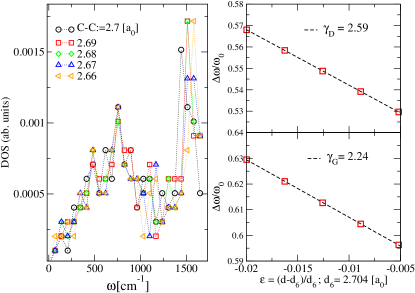
Figure 11: Left panel: Phonon density of states for the flake of size $N{=}6$. Data sets are shown for different C-C bond distances. Upper right panel shows the flow of D-peak with in-plane strain. Lower right panel shows the variation of Raman G-peak with strain, where $\omega_{0}$ is the Raman band frequency($\approx$ 2680 ${\rm cm}^{-1}$)Ni et al. (2008). The corresponding vibration modes are shown in Fig. 12.

While the sign of $\gamma_{h,u}$ was not unexpected, it is noteworthy that the vibrational contributions to the phenomenological material parameters are actually not so small. The bare electronic bending rigidity, $\kappa_{\rm el}$ is reduced by as much as 26% down to $\kappa{=}\kappa_{\rm el}+\gamma_{h}{=}0.88$eV. Similarly, when expressing the effect of vibrations on the atomic lattice as an effective strain pushing the atoms to larger distances, then this strain reaches values up to 0.4%.

Here, we also calculate the Grüneisen parameters associated with individual modes (see Fig. 12). The right panel in Fig. 11 shows the flow of the Raman frequencies (upper half D, lower G) with the applied strain. The frequency decreases linearly (as described in Eq. (17)) with decreasing compression due to anharmonicity of the interatomic potential. The slope essentially estimates the Grüneisen parameters, $\gamma_{\rm G}$ and $\gamma_{\rm D}$ for the vibrations shown in Fig. 12. Our results for $\gamma_{\rm G}$, $\gamma_{\rm D}$ are consistent with the earlier experiments and first principal calculations (see Tab. 6) available in literatureMounet and Marzari (2005); Thomsen et al. (2002); Proctor et al. (2009); Mohiuddin et al. (2009).

Figure 12: Schematic diagram of vibrating modes that give rise to D(left) and G(right) peaks in Raman spectra of graphene.

VI Conclusion

The elastic properties of edge hydrogenated graphene flakes have been investigated employing the density functional theory (DFT). Our study emphasizes the interplay between the edge and bulk properties which are mediated via long range elastic forces.

Specifically, we are able to disentangle bulk, surface and corner contributions to the free energy together with the leading higher order corrections. The binding energy per surface (edge) bond (7.5eV) is roughly two eV higher than the one for interior (bulk) bonds (5.2eV); similarly, edge bonds have a tendency to be shorter than bulk ones. As a consequence, the flake’s interior undergoes a surface induced compression which is the more pronounced the smaller the flake is. This compression manifests itself in the way in which various observables depend on the flake size, $N$. For example, elastic constants (i.e. Lamé parameters) of small flakes can exceed their bulk limit ($\mu+\lambda\approx 70$eV per ring, $\mu\approx 51$eV per ring, $\nu=0.162$) by 30% ($\mu+\lambda$) or even by 70% ($\mu$). In comparison, the sheet (out of plane, buckling) stiffness, $\kappa\approx 1.2$eV, is less sensitive to $N$. Non-linearities remain weak (less than 10% increase) as long as the ratio of out of plane amplitude and in plane wavelength of buckling is below 5%. To highlight the importance of quantum effects on elasticity we have also calculated the vibrational spectrum of graphene flakes. Quantum corrections affect mostly the sheet stiffness, $\kappa$, lowering it significantly, about 26% within our DFT framework.

Finally, based on these results we predict a pronounced shift of the Raman G- and D-peaks with decreasing flake size to higher values. It is a natural consequence of the edge induced flake compression. The associated Grüneisen parameters are $\gamma_{\rm D}\approx 2.6$eV/$\AA^{2}$ and $\gamma_{\rm G}=2.2$eV/$\AA^{2}$.

VII Acknowledgments

We are grateful to A. Bagrets, M. van Setten and V. Meded for helping us with the data visualization and also with the ab-initio calculation. We are thankful to J. Weissmüller for numerous discussions during this work. Also, we acknowledge support from the Landesgraduiertenförderung Baden-Württemberg and Center of Functional Nanostructures of the Deutsche Forschungsgemeinschaft, project 4.11.

References

- Novoselov et al. (2004) K. S. Novoselov, A. K. Geim, S. V. Morozov, D. Jiang, Y. Zhang, S. V. Dubonos, I. V. Grigorieva, and A. A. Firsov, Science 306, 666 (2004).
- Zhang et al. (2005) Y. Zhang, Y.-W. Tan, H. L. Stormer, and P. Kim, Nature 438, 201 (2005).
- Novoselov et al. (2006) K. S. Novoselov, E. McCann, S. V. Morozov, V. I. Fal’ko, M. I. Katsnelson, U. Zeitler, D. Jiang, F. Schedin, and A. K. Geim, Nature Phys. 2, 177 (2006).
- Geim and Novoselov (2007) A. K. Geim and K. S. Novoselov, Nature Mater. 6, 183 (2007).
- Novoselov et al. (2005) K. S. Novoselov, D. Jiang, F. Schedin, T. J. Booth, V. V. Khotkevich, S. V. Morozov, and A. K. Geim, Proc. Natl. Acad. Sci. 102, 1045 (2005).
- Castro Neto et al. (2009) A. H. Castro Neto, F. Guinea, N. M. R. Peres, K. S. Novoselov, and A. K. Geim, Rev. Mod. Phys. 81, 109 (2009).
- Nakada et al. (1996) K. Nakada, M. Fujita, G. Dresselhaus, and M. S. Dresselhaus, Phys. Rev. B 54, 17954 (1996).
- Stampfer et al. (2009) C. Stampfer, J. Güttinger, S. Hellmüller, F. Molitor, K. Ensslin, and T. Ihn, Phys. Rev. Lett. 102, 056403 (2009).
- Fujita et al. (1996) M. Fujita, K. Wakabayashi, K. Nakada, and K. Kusakabe, J. Phys. Soc. Jap. 65, 1920 (1996).
- Brey and Fertig (2006) L. Brey and H. A. Fertig, Phys. Rev. B 73, 235411 (2006).
- Wakabayashi et al. (1998) K. Wakabayashi, M. Sigrist, and M. Fujita, J. Phys. Soc. Jap. 67, 2089 (1998).
- Son et al. (2006a) Y.-W. Son, M. L. Cohen, and S. G. Louie, Nature 444, 347 (2006a).
- Son et al. (2006b) Y.-W. Son, M. L. Cohen, and S. G. Louie, Phys. Rev. Lett. 97, 216803 (2006b).
- Hod et al. (2007a) O. Hod, V. Barone, J. E. Peralta, and G. E. Scuseria, Nano Lett. 7, 2295 (2007a).
- jun Kan et al. (2008) E. jun Kan, Z. Li, J. Yang, and J. G. Hou, J. Am. Chem. Soc. 130, 4224 (2008).
- Peres et al. (2006) N. M. R. Peres, A. H. Castro Neto, and F. Guinea, Phys. Rev. B 73, 195411 (2006).
- Pisani et al. (2007) L. Pisani, J. A. Chan, B. Montanari, and N. M. Harrison, Phys. Rev. B 75, 064418 (2007).
- en Jiang et al. (2007) D. en Jiang, B. G. Sumpter, and S. Dai, J. Chem. Phys. 127, 124703 (2007).
- Fernández-Rossier and Palacios (2007) J. Fernández-Rossier and J. J. Palacios, Phys. Rev. Lett. 99, 177204 (2007).
- Wang et al. (2009) W. L. Wang, O. V. Yazyev, S. Meng, and E. Kaxiras, Phys. Rev. Lett. 102, 157201 (2009).
- G mez-Navarro et al. (2008) C. G mez-Navarro, M. Burghard, and K. Kern, Nano Lett. 8, 2045 (2008).
- Danneau et al. (2008) R. Danneau, F. Wu, M. F. Craciun, S. Russo, M. Y. Tomi, J. Salmilehto, A. F. Morpurgo, and P. J. Hakonen, Phys. Rev. Lett. 100, 196802 (2008).
- Lauffer et al. (2008) P. Lauffer, K. V. Emtsev, R. Graupner, T. Seyller, L. Ley, S. A. Reshanov, and H. B. Weber, Phys. Rev. B 77, 155426 (2008).
- Li et al. (2008) X. Li, X. Wang, L. Zhang, Lee, Sangwon, and H. Dai, Science 319, 1229 (2008).
- Haluka et al. (2007) M. Haluka, D. Obergfell, J. C. Meyer, G. Scalia, G. Ulbricht, B. Krauss, D. H. Chae, T. Lohmann, M. Lebert, M. Kaempgen, et al., Phys. Status Solidi (b) 244, 4143 (2007).
- Miao et al. (2007) F. Miao, S. Wijeratne, Y. Zhang, U. C. Coskun, W. Bao, and C. N. Lau, Science 317, 1530 (2007).
- Casiraghi et al. (2009) C. Casiraghi, A. Hartschuh, H. Qian, S. Piscanec, C. Georgi, A. Fasoli, K. S. Novoselov, D. M. Basko, and A. C. Ferrari, Nano Lett. 9 (2009).
- de Parga et al. (2008) A. L. V. de Parga, F. Calleja, B. Borca, J. M. C. G. Passeggi, J. J. Hinarejos, F. Guinea, and R. Miranda, Phys. Rev. Lett. 100, 056807 (2008).
- Tan et al. (2009) C. L. Tan, Z. B. Tan, K. Wang, L. Ma, F. Yang, F. M. Qu, J. Chen, C. L. Yang, and L. Lu (2009), eprint arXiv/0910.5777.
- Fasolino et al. (2007) A. Fasolino, J. H. Los, and M. I. Katsnelson, Nature Materials 6, 858 (2007).
- Gui et al. (2008) G. Gui, J. Li, and J. Zhong, Phys. Rev. B 78, 075435 (2008).
- Atalaya et al. (2008) J. Atalaya, A. Isacsson, and J. M. Kinaret, Nano Lett. 8, 4196 (2008).
- Garcia-Sanchez et al. (2008) D. Garcia-Sanchez, A. M. van der Zande, A. S. Paulo, B. Lassagne, P. L. McEuen, and A. Bachtold, Nano Lett. 8, 1399 (2008).
- Lee et al. (2008) C. Lee, X. Wei, J. W. Kysar, and J. Hone, Science 321, 385 (2008).
- Pereira et al. (2009) V. M. Pereira, A. H. Castro Neto, and N. M. R. Peres, Phys. Rev. B 80, 045401 (2009).
- Choi et al. (2010) S.-M. Choi, S.-H. Jhi, and Y.-W. Son, Phys. Rev. B 81, 081407 (2010).
- Zakharchenko et al. (2009) K. V. Zakharchenko, M. I. Katsnelson, and A. Fasolino, Phys. Rev. Lett. 102, 046808 (2009).
- Hod and Scuseria (2009) O. Hod and G. E. Scuseria, Nano Lett. 9, 2619 (2009).
- Cadelano et al. (2009) E. Cadelano, P. L. Palla, S. Giordano, and L. Colombo, Phys. Rev. Lett. 102, 235502 (2009).
- Guinea et al. (2009) F. Guinea, B. Horovitz, and P. Le Doussal, Solid State Commun 149, 1140 (2009).
- Reddy et al. (2009) C. D. Reddy, A. Ramasubramaniam, V. B. Shenoy, and Y.-W. Zhang, Appl. Phys. Lett. 94, 101904 (2009).
- Lu et al. (2009) Q. Lu, M. Arroyo, and R. Huang, J. Phys. D: Appl. Phys. 42, 102002 (6pp) (2009).
- Ribeiro et al. (2009) R. M. Ribeiro, V. M. Pereira, N. M. R. Peres, P. R. Briddon, and A. H. Castro Neto, New J. Phys. 11, 115002 (2009).
- Meyer et al. (2007) J. C. Meyer, A. K. Geim, M. I. Katsnelson, K. S. Novoselov, T. J. Booth, and S. Roth, 446, 60 (2007).
- Stolyarova et al. (2007) E. Stolyarova, K. Rim, S. Ryu, J. Maultzsch, P. Kim, L. Brus, T. Heinz, M. Hybertsen, and G. Flynn, Proc. Natl. Acad. Sci. 104 (2007).
- Ishigami et al. (2007) M. Ishigami, J. H. Chen, W. G. Cullen, M. S. Fuhrer, and E. D. Williams, Nano Lett. 7, 1643 (2007).
- Bao et al. (2009) W. Bao, F. Miao, Z. Chen, H. Zhang, W. Jang, C. Dames, and C. N. Lau, Nat. Nano. 4, 562 (2009).
- Mohiuddin et al. (2009) T. M. G. Mohiuddin, A. Lombardo, R. R. Nair, A. Bonetti, G. Savini, R. Jalil, N. Bonini, D. M. Basko, C. Galiotis, N. Marzari, et al., Phys. Rev. B 79, 205433 (2009).
- Chen et al. (2009) C. C. Chen, W. Bao, J. Theiss, C. Dames, C. N. Lau, and S. B. Cronin, Nano Lett. (2009).
- Ferrari et al. (2006) A. C. Ferrari, J. C. Meyer, V. Scardaci, C. Casiraghi, M. Lazzeri, F. Mauri, S. Piscanec, D. Jiang, K. S. Novoselov, S. Roth, et al., Phys. Rev. Lett. 97, 187401 (2006).
- Ni et al. (2008) Z. H. Ni, T. Yu, Y. H. Lu, Y. Y. Wang, Y. P. Feng, and Z. X. Shen, ACS Nano 2, 2301 (2008).
- Proctor et al. (2009) J. E. Proctor, E. Gregoryanz, K. S. Novoselov, M. Lotya, J. N. Coleman, and M. P. Halsall, Phys. Rev. B 80, 073408 (2009).
- Tsoukleri et al. (2009) G. Tsoukleri, J. Parthenios, K. Papagelis, R. Jalil, A. C. Ferrari, A. K. Geim, K. S. Novoselov, and C. Galiotis, Small 5, 2397 (2009).
- Reich et al. (2000) S. Reich, H. Jantoljak, and C. Thomsen, Phys. Rev. B 61, R13389 (2000).
- Sánchez-Portal et al. (1999) D. Sánchez-Portal, E. Artacho, J. M. Soler, A. Rubio, and P. Ordejón, Phys. Rev. B 59, 12678 (1999).
- Reich et al. (2002) S. Reich, C. Thomsen, and P. Ordejón, Phys. Rev. B 65, 153407 (2002).
- Hod et al. (2007b) O. Hod, J. E. Peralta, and G. E. Scuseria, Phys. Rev. B 76, 233401 (2007b).
- Landau and Lifshitz (1959) L. Landau and E. Lifshitz, Theory of Elasticity, Vol 7 (Pergamon Press, 1959).
- Ahlrichs et al. (1989) R. Ahlrichs, M. Bär, M. Häser, H. Horn, and C. Kölmel, Chem. Phys. Lett. 162, 165 (1989).
- Becke (1988) A. D. Becke, Phys. Rev. A 38, 3098 (1988).
- Perdew (1986) J. P. Perdew, Phys. Rev. B 33, 8822 (1986).
- Perdew and Wang (1992) J. P. Perdew and Y. Wang, Phys. Rev. B 45, 13244 (1992).
- Perdew et al. (1996) J. P. Perdew, K. Burke, and M. Ernzerhof, Phys. Rev. Lett. 77, 3865 (1996).
- Becke (1993) A. D. Becke, J Chem. Phys. 98, 5648 (1993).
- Schäfer et al. (1992) A. Schäfer, H. Horn, and R. Ahlrichs, J Chem. Phys. 97, 2571 (1992).
- Mounet and Marzari (2005) N. Mounet and N. Marzari, Phys. Rev. B 71, 205214 (2005).
- Kudin et al. (2001) K. N. Kudin, G. E. Scuseria, and B. I. Yakobson, Phys. Rev. B 64, 235406 (2001).
- Arroyo and Belytschko (2004) M. Arroyo and T. Belytschko, Phys. Rev. B 69, 115415 (2004).
- Weast and Astle (2009) R. C. Weast and M. J. Astle, CRC Handbook of Chemistry and Physics (CRC press, New York, 2009), 89th ed.
- Blakslee et al. (1970) O. L. Blakslee, D. G. Proctor, E. J. Seldin, G. B. Spence, and T. Weng, J. Appl. Phys. 41, 3373 (1970).
- Bosak et al. (2007) A. Bosak, M. Krisch, M. Mohr, J. Maultzsch, and C. Thomsen, Phys. Rev. B 75, 153408 (2007).
- Odegard et al. (2002) G. M. Odegard, T. S. Gates, L. M. Nicholson, and K. E. Wise, Compos. Sci. Technol. 62, 1869 (2002).
- Deglmann et al. (2002) P. Deglmann, F. Furche, and R. Ahlrichs, Chem. Phys. Lett. 362, 511 (2002).
- Deglmann and Furche (2002) P. Deglmann and F. Furche, J. Chem. Phys. 117, 9535 (2002).
- Thomsen et al. (2002) C. Thomsen, S. Reich, and P. Ordejón, Phys. Rev. B 65, 073403 (2002).