A multiwavelength study of star formation in the vicinity of Galactic region Sh 2-100

Abstract

We present multiwavelength investigation of morphology, physical-environment, stellar contents and star formation activity in the vicinity of star-forming region Sh 2-100. It is found that the Sh 2-100 region contains seven regions of ultracompact and compact nature. The present estimation of distance for three regions, along with the kinematic distance for others, suggests that all of them belong to the same molecular cloud complex. Using near-infrared photometry, we identified the most probable ionizing sources of six regions. Their approximate photometric spectral type estimates suggest that they are massive early-B to mid-O zero-age-main-sequence stars and agree well with radio continuum observations at 1280 MHz, for sources whose emissions are optically thin at this frequency. The morphology of the complex shows a non-uniform distribution of warm and hot dust, well mixed with the ionized gas, which correlates well with the variation of average visual extinction ($\sim$ 4.2 - 97 mag) across the region. We estimated the physical parameters of ionized gas with the help of radio continuum observations. We detected an optically visible compact nebula located to the south of the 850 $\mu$m emission associated with one of the regions and the diagnostic of the optical emission line ratios gives electron density and electron temperature of $\sim$ 0.67 $\times$ 10³ cm^-3 and $\sim$ 10⁴ K, respectively. The physical parameters suggest that all the regions are in different stages of evolution, which correlate well with the probable ages in the range $\sim$ 0.01 - 2 Myr of the ionizing sources. The spatial distribution of infrared excess stars, selected from near-infrared and IRAC color-color diagrams, correlates well with the association of gas and dust. The positions of infrared excess stars, ultracompact and compact regions at the periphery of an H i shell, possibly created by a WR star, indicate that star formation in Sh 2-100 region might have been induced by an expanding H i shell.

1 Introduction

Massive star formation is poorly understood as compared to low-mass stars, because their formation takes place in the dense core of a molecular cloud of high visual extinction, usually observable at far-infrared (FIR) to millimeter wavelengths and their evolutionary time scales are much shorter ($\leq$ 10⁵ yr) (e.g., Bernasconi & Maeder 1996). The radio free-free emission in terms of ultracompact (UCH ii ) regions, represents a later evolutionary sequence of a massive protostar outlined by Beuther et al. (2007), where the associated high mass protostar may still be in the accretion phase (e.g, Shepherd & Churchwell 1996) or has already ceased the accretion (Garay & Lizano 1999). The UCH ii region can further evolve into the less obscure stage of compact (CH ii ) and classical regions (Garay & Lizano 1999) by the disruption of associated gas and dust, revealing both, the embedded high-mass and lower mass stellar population at shorter wavelengths. Most of the high-mass star-forming regions in the Galaxy lie at a distance of more than 1 kpc. As a result, the problem in interpreting observations of massive star formation originates in source confusion at the core of distant molecular clouds due to their cluster mode formation. Statistically, it has been shown that the most luminous protostars form in molecular clouds associated with evolved regions (Dobashi et al. 2001), where the interplay between the stars’ radiation field and associated gas and dust makes the environment even more complex. Therefore, a detailed study of the star-forming region hosting young massive stars, using optical, near-infrared (NIR), mid-infrared (MIR) and radio bands, is necessary to understand the high-mass star formation scenario in these complexes.

In this paper, we have studied a young star-forming region (SFR) K3-50 shown in Fig. 1, which contains a group of regions, namely A, B, C, D, E, and F (cf. Israel 1976). The region C itself consists of two UCH ii regions, C1 and C2 (Harris 1975). The kinematic distance towards K3-50 ranges from 7.9 to 9.3 kpc (Harris 1975; Bronfman et al. 1996; Araya et al. 2002). In the present study we have adopted a widely used value of distance of $\sim$ 8.7 kpc for our analysis. We also derived distances of three regions that come out to be close to the value of 8.7 kpc. The group of regions is located within an area of radius $\sim$ 3^′.5 centered on $\alpha_{2000}=20^{h}01^{m}42^{s}$, $\delta_{2000}=+33^{\circ}33^{\prime}49^{\prime\prime}$, in the proximity of an evolved diffuse nebula Sh 2-100 of $\sim$ 4^′ in size (Sharpless 1959). Sh 2-100 is itself a part of the large molecular cloud complex W58, which consists of several classes of regions with widely varying physical parameters. The observed radio luminosity of the complex can be explained by the presence of OB association (cf. Israel 1976). In Fig. 1 one can notice that K3-50D, K3-50E, and K3-50F are associated with nebulosity. A faint nebulosity is also seen $\sim$ 15.5^′′ away in the southern direction of K3-50C2, whereas K3-50A appears as a stellar point-like source and is marked with a circle. The regions K3-50B and K3-50C1 are optically invisible radio sources, implying that the extinction is high enough to obscure the regions. By comparing the expected infrared Br$\alpha$ line fluxes as predicted from radio continuum fluxes, to the observed Br$\alpha$ line fluxes, Roelfsema et al. (1988) estimated visual extinction of 15, 26, 97 and 32 mag towards A (over 25^′′ aperture), B (over 5^′′ aperture), C1 and C2 (over 15^′′ aperture) respectively, while the extinction towards D was found to be 2 mag (5^′′ aperture). Observations at radio wavelengths suggest that these regions harbor at least one massive OB star (Harris 1975; Israel 1976; DePree et al. 1994). The UCH ii regions, astronomical masers, outflows, detection of high density tracer molecules and infrared (IR) sources with IR-excess are the trademarks of young star-forming regions. The evidence of weak bipolar molecular outflow by Phillips & Mampaso (1991) with CO $J$ = 2 - 1 transition, ionized outflow by DePree et al. (1994) with H76 alpha radio recombination line, detection of molecular core mapped in the HCO⁺ and CS (2-1) lines by Vogel & Welch (1983) and Bronfman et al. (1996) suggest the youthfulness of the Sh 2-100 region. These observations along with the presence of astronomical masers (H₂O by Kurtz & Hofner 2005; OH by Baudry & Desmurs 2002) imply active star formation is going on around Sh 2-100. The current star formation activity in the vicinity of Sh 2-100 region is probably the effect of feedback from the earlier generation stars of the W58 complex (Israel 1980).

Though there are several studies in the radio and infrared domain, most of them are concentrated on K3-50A and K3-50C. To continue our multiwavelength investigations of massive SFRs (cf. Ojha et al. 2004a; Ojha et al. 2004b; Ojha et al. 2004c; Tej et al. 2006; Samal et al. 2007; Pandey et al. 2008), we have studied an area of 8^′ $\times$ 8^′ of Sh 2-100 region to understand the star formation activity in this region. This paper presents new results from optical and infrared photometry, optical spectroscopy and low frequency radio continuum observations. Based on these observations, we have carried out a detailed study of the ionizing sources of individual regions, physical characteristics and the nature of associated lower mass population. With the following layout of the paper we tried to interpret the possible star formation scenario of W58 cloud complex. In Sect. 2, we describe our observations and the reduction procedures. In Sect. 3, we discuss other available datasets used in the present study. Sect. 4 describes the general morphology of the region. Sect. 5 describes the infrared and radio components associated with the region. In Sect. 6, we discuss the nature of individual regions. Sect. 7 is devoted to general discussion and star formation scenario in W58 complex. We present the main conclusions of our results in Sect. 8.

2 Observations and data reduction

2.1 Optical photometry

$UBV$ CCD photometric observations were performed for the Sh 2-100 region on 2006 October 24 and 25, using the 2K $\times$ 2K CCD system at the f/13 Cassegrain focus of the 104-cm Sampurnanand telescope (ST) of ARIES, Nainital (India). The 0.37 arcsec pixel^-1 plate scale gives a field of view (FOV) of $\sim$ 12${}^{\prime}.6\times 12^{\prime}.6$ on the sky. The observing conditions were photometric and the average FWHM during the observing period was $\sim$ 1^′′.7- 2^′′.0. To improve the signal-to-noise (S/N) ratio, observations were made in 2 $\times$ 2 pixel binning mode. Several bias frames and twilight flat field exposures were taken during the observations. We observed the standard area SA101 (Landolt 1992) on 2006 October 25 several times during the night to determine the atmospheric extinction coefficients and to calibrate the CCD systems. The initial processing of the CCD images was done using the IRAF data reduction package. Then, for a given filter, frames of same exposure time were co-added to improve the S/N. Photometric measurements of the stars were performed using DAOPHOT II package of MIDAS. The stellar images were well sampled and a variable point spread function (PSF) was applied from several uncontaminated stars present in the frames. The calibration from instrumental to standard system was done using the procedure outlined by Stetson (1987). The standardization residuals between the standard and transformed $V$ magnitude and colors are less than 0.02 mag. We used only those stars having photometric error in magnitudes $\leq 0.1$ in the present analyses.

2.2 Optical spectroscopy

Using the Himalaya Faint Object Spectrograph Camera (HFOSC) available with the 2.01 m Himalayan Chandra Telescope (HCT), operated by the Indian Institute of Astrophysics, Bangalore (India), we obtained optical spectra of possible ionizing sources of K3-50D, K3-50B and optical nebula associated with K3-50A on 2007 June 18 and 2007 October 29. The instrument is equipped with a SITe 2K $\times$ 4K pixel CCD. The central 2K $\times$ 2K region is used for imaging which corresponds to a FOV of $\sim$ $10^{\prime}$ $\times$ $10^{\prime}$, with a pixel size of 0^′′.3. The spectra were obtained with a grism (Gr 7) in the wavelength range of 3500-7000 Å at a spectral dispersion of 1.45 Å pixel^-1. The exposure time was 900s for each source. The spectroscopic observations were carried out under good photometric sky conditions. The one-dimensional spectra were extracted from the bias-subtracted and flat-field corrected images using the optimal extraction method (Horne 1986) of IRAF. Wavelength calibration of the spectra was done using FeAr lamp source to identify emission lines of the lamp and we fitted a lower order polynomial to find a dispersion solution. For flux calibration of the nebular spectrum, we used spectrophotometric standard star BD 284211 (Massey et al. 1988) observed on the same night.

2.3 Near-Infrared Observations

Imaging observations of the Sh 2-100 region centered on $\alpha_{2000}=20^{h}01^{m}44^{s}$, $\delta_{2000}=+33^{\circ}33^{\prime}07^{\prime\prime}$, in $J$ ($\lambda$ = 1.25 $\mu$m), $H$ ($\lambda$ = 1.63 $\mu$m), and $K_{\rm s}$ ($\lambda$ = 2.14 $\mu$m) bands were obtained on 2008 July 21 with the 1.4 m Infrared Survey Facility (IRSF) telescope and SIRIUS, a three-color simultaneous camera equipped with three 1024 $\times$ 1024 HgCdTe arrays. The FOV in each band is $\sim$ 7^′.8 $\times$ 7^′.8, with a pixel scale of 0^′′.45 at the f/10 Cassegrain focus. Further details of the instrument are given in Nagashima et al. (1999) and Nagayama et al. (2003). A sky field was also observed centered on $\alpha_{2000}=20^{h}00^{m}44^{s}$, $\delta_{2000}=+33^{\circ}31^{\prime}36^{\prime\prime}$ and used for sky subtraction. We obtained 120 dithered frames each of 10s, thus giving a total integration time of 1200s in each band. The observing conditions were photometric and the average FWHM during the observing period was $\sim$ 1^′′.8-2^′′.0. Data reduction was done using pipeline software based on IRAF package tasks. Dome flat-fielding and sky subtraction with a median sky frame were applied. Photometry of point sources was performed using the PSF algorithm ALLSTAR in the DAOPHOT package (Stetson 1987) within the IRAF environment. The PSF was determined from 15 relatively bright and isolated stars of the field. We used an aperture radius of 1 FWHM, with appropriate aperture corrections per band for the final photometry.

For photometric calibration, we used 54 isolated 2MASS Point Source Catalog (PSC) sources (see §3.1) with $K_{\rm s}$ mag range 12-14 and having error $<$ 0.05 mag. The same 2MASS sources were used for absolute position calibration and a position accuracy of better than $\pm$0^′′.1 was achieved. The sources with $K_{\rm s}$ mag $<$ 11 were saturated in our image. For such bright sources, 2MASS PSC data were used. For one source (i.e., a possible ionizing source of K3-50A), we have used the data (star id 68) from Alvarez et al. (2004), since the source was found to be $\approx$ 1.3 mag and 2.2 mag brighter than $K$-band and $H$-band, respectively, than in Alvarez et al. (2004). Alvarez et al. (2004) observation covers an area of $\sim$ 80^′′ $\times$ 80^′′ in the vicinity of K3-50A with a resolution (FWHM) of 0^′′.22. A comparison of present photometry with that of 2MASS photometry as a function of $J$ mag for the common sources is shown in Fig. 2, where the 2MASS sources of photometric error $\leq$ 0.1 mag and ‘read-flag’ values between 1 to 3 are selected to ensure good quality. We find that the photometric scatter in magnitude increases at the fainter end, whereas the mean photometric uncertainties are $\leq$ 0.1 in all the three bands. To plot the data in color-color (CC) and color-magnitude (CM) diagrams, the $JHK_{\rm s}$ data were transformed to California Institute of Technology (CIT) system using the relation given at the 2MASS website.

2.4 Optical and NIR narrow-band imaging

Optical CCD narrow-band images of the nebula around Sh 2-100 region were obtained in H$\alpha$ ($\lambda$ = 6563 Å, $\Delta\lambda$ = 100 Å) and [S II] ($\lambda$= 6724 Å, $\Delta\lambda$ = 100 Å) on 2007 June 18 with HFOSC on the HCT. We used $R$-band as a nearby continuum for the continuum subtraction.

Narrow-band NIR observations were carried out in $Br\gamma$  ($\lambda$ = 2.16 $\mu$m, $\Delta\lambda$ = 0.019 $\mu$m) and $K$ continuum ($\lambda$ = 2.264 $\mu$m, $\Delta\lambda$ = 0.054 $\mu$m) with HCT on 2004 October 10, using the NIR imager (NIRCAM), which is a 0.8 - 2.5 $\mu$m camera with 512 $\times$ 512 HgCdTe array. For our observations, the NIRCAM was used in the Camera-B mode which has a FOV of $\sim$ 3^′.6 $\times$ 3^′.6. We obtained several dithered (by $20^{\prime\prime}$) frames of the target centered on $\alpha_{2000}=20^{h}01^{m}47^{s}$, $\delta_{2000}=+33^{\circ}31^{\prime}38^{\prime\prime}$ in order to remove bad pixels, cosmic rays and to eliminate the presence of objects with extended emission for construction of sky images. Typical integration times per frame were 90s, and 20s in the $Br\gamma$, and $K$ continuum bands, respectively. The images were co-added to obtain the final image in each band. We also obtained several dithered sky frames close to the target position in both the bands. All images were bias and dark-subtracted and flat-field corrected. The continuum subtraction of the images was done after aligning and PSF matching.

Details of the log of observations are given in Table 1.

2.5 Radio continuum observations

In order to probe the ionized gas component, radio continuum interferometric observations at 1280 MHz and 610 MHz were carried out on 2004 January 25 and 2004 April 07, using Giant Metrewave Radio Telescope (GMRT) array. The GMRT has a “Y”-shaped hybrid configuration of 30 antennae, each 45 m in diameter. There are six antennae along each of the three arms (with arm length of $\sim$ 14 km). The rest of the twelve antennae are located in a random and compact $\rm 1\times 1$ $\rm km^{2}$ arrangement near the center. Details of the GMRT antennae and their configurations can be found in Swarup et al. (1991). The largest angular scales to which the GMRT is sensitive are 8^′ and 17^′ at 1280 and 610 MHz, respectively.

The flux and phase calibrators were observed in order to derive the phase and amplitude gains of the antennae and the details of the observations are given in Table. 2. 3C48 and 3C286 were used as the flux calibrators with assumed flux densities of 17.23 Jy at 1280 MHz and 21.03 Jy at 610 MHz, respectively. The phase calibrators were 2052+365 at 1280 MHz and 1924+334 at 610 MHz observations, with a bootstrapped flux density of 9.59 Jy and 6.03 Jy, respectively. The data analysis was done using AIPS. The estimated uncertainty of the flux calibration is within 7% at both frequencies. The image of the field was formed by Fourier inversion and cleaning algorithm task IMAGR. The high resolution images ($\sim$ 3^′′.3 $\times$ 3^′′.0 at 1280 MHz and $\sim$ 5^′′.5 $\times$ 4^′′.8 at 610 MHz) were made with a Briggs weighting function (robust factor = -1 to 0) halfway between uniform and natural weighting. Few iterations of self-calibration were carried out to remove the residual effects of atmospheric and ionospheric phase corruptions and to obtain improved maps. The system temperature correction was done using sky temperature from the 408 MHz map of Haslam et al. (1982). A correction factor equal to the ratio of the system temperature toward the source and flux calibrator has been used to scale the deconvolved images.

3 Other Available Data Sets

3.1 Near-Infrared Data from $2MASS$

For the IRSF photometric calibration, study of the bright end of the stellar population and astrometric calibration, we used 2MASS PSC (Cutri et al. 2003) in the $J$ (1.25 $\mu$m), $H$ (1.65 $\mu$m) and $K{\rm{}_{s}}$ (2.17 $\mu$m) bands. The 2MASS data have positional accuracy of better than $2^{\prime\prime}$. Our source selection was based on the ‘read-flag’ values of “1”, “2” or “3”, which generally indicate the best quality detections, photometry and astrometry (http://www.ipac.caltech.edu/2mass/releases/allsky/doc).

3.2 Mid-infrared data from Spitzer

The archived MIR data for the region were obtained with the Infrared Array Camera (IRAC; Fazio et al. 2004a) on board the Spitzer Space Telescope. The Basic Calibrated Data (BCD) images were downloaded from the Spitzer Space Telescope Archive using the Leopard package. The IRAC observations of the region were taken on 2005 October 22 (Program ID 20778, AOR key 15154944: A Young Stellar and Protostellar Census of Galactic Ultracompact Regions, PI: S. Carey). Mosaics were built at the native instrument resolution of 1^′′.2 per pixel with the standard BCDs using the MOPEX (Mosaicker and Point Source Extractor) software provided by Spitzer Science Center. To perform photometry with the DAOPHOT package provided within the IRAF environment, we first converted the pixel values of IRAC images, which are in MJy/sr units to DN/s using the conversion factor given in the “IRAC Data Handbook” version 3.0 (http://ssc.spitzer.caltech.edu/irac/dh/). We performed aperture photometry on the IRAC images with a source detection at the 5$\sigma$ level above the average local background. Due to the crowded nature of the field, an aperture radius of 2 pixels and a sky annulus extending from 2 to 6 pixels were used. The zero point magnitudes and appropriate aperture corrections were taken from the the “IRAC Data Handbook” version 3.0 for the final photometry. The detected sources were examined visually in each band to clean the sample of non-stellar objects and false detections around bright stars. We accepted good detections as those sources which have photometric uncertainties less than 0.2 mag.

3.3 Mid-infrared data from $MSX$

The Midcourse Space Experiment (MSX) surveyed the entire Galactic plane within $|$$b$$|$ $\leq$ 5^∘ in four MIR bands centered at 8.28 $\mu$m (A), 12.13 $\mu$m (C), 14.65 $\mu$m (D) and 21.34 $\mu$m (E) at a spatial resolution of 18^′′.3 (Price et al. 2001) and a global absolute astrometric accuracy of about 1^′′.9 (Egan et al. 2003). Point sources have been searched around Sh 2-100 region from MSX PSC Version 2.3 (Egan et al. 2003).

3.4 Mid- and far-infrared data from $IRAS-HIRES$

The data from the Infrared Astronomical Satellite ($IRAS$) survey in the two bands (25 and 60 $\mu$m ) for the region around Sh 2-100 were HIRES-processed (Aumann et al. 1990) at the Infrared Processing and Analysis Center (IPAC), Caltech, to obtain high angular resolution maps. We used $IRAS$-HIRES maps to generate the intensity distribution map due to thermal emission from the dust component around Sh 2-100.

4 General Morphology around Sh 2-100

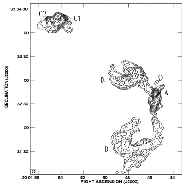
Figure 5: High resolution radio continuum map at 1280 MHz for the region around Sh 2-100 with a resolution of $\rm 3\arcsec.3\times 3\arcsec.0$. The contour levels are at 2.2 $\times$ (3, 4, 6, 8, 12, 16, 20, 24, 30, 36) mJy/beam, where $\sim$ 2.2 mJy/beam is the rms noise in the map. The labelled axes are in J2000 coordinates. Individual regions are also marked.

Fig. 3 represents a false $JHK_{\rm s}$ color-composite image ($J$, blue; $H$, green; and $K_{\rm s}$, red) of Sh 2-100 region, which reveals prominent nebulosities associated with the marked regions except K3-50C1, indicating that the extinction in the molecular cloud towards C1 is high enough to attenuate the emission at 2.14 $\mu$m. A dark lane is also observed in the direction of K3-50C2, bisecting its diffuse nebulosity into north and south components, which extend towards K3-50C1. A bridge between K3-50D and K3-50A is also seen in Fig. 3, which is not visible in POSS II image (Fig. 1), suggesting that the extinction is high towards north-western side of K3-50D. Fig. 3 also displays several red sources indicating the presence of young stellar sources still deeply embedded in the molecular cloud, whereas bluest stars are likely to be evolved/foreground objects of the field. The background objects would also appear red, but the locations of high column density regions should minimize the contamination of such objects. Fig. 4 shows contours of the 610 MHz radio free-free emission overlaid onto the IRSF $K_{\rm s}$-band image. In the $K_{\rm s}$-band image, the regions of recent star formation are traced by the bright nebulosity, whereas the regions detected in centimeter surveys of the cloud trace high-mass star formation. It is well established that formation of high mass stars in young complexes is accompanied with the simultaneous or subsequent formation of less massive sources, which can be studied in NIR (Persi et al. 2000). Our high angular resolution radio map at 1280 MHz is shown in Fig. 5, which was made with the robust parameter equal to -1, to see more compact emission features. In Fig. 5 one can notice a non-uniform distribution of free-free emission, indicating that Sh 2-100 is morphologically a complex region. The low brightness components K3-50E and K3-50F are resolved out in our high resolution map at 1280 MHz (Fig. 5). We therefore made a low resolution map ($\sim$ $\rm 44\arcsec\times 27\arcsec$) using uv range up to 10 $k\lambda$ with a robust parameter equal to 0, to recover the weak diffuse emission associated to these sources as seen in 610 MHz map. The resulting map is discussed in §6.5. On the other hand, 1280 MHz high resolution map partially resolves two UCH ii regions of K3-50C, which are not resolved in our 610 MHz map.

5 Infrared and Radio Properties of the Sh 2-100 star-forming region

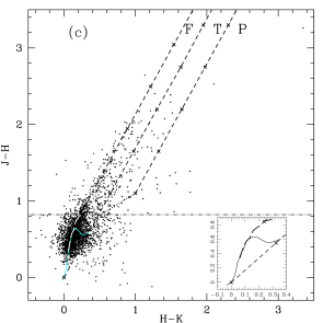
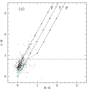
Figure 6: (a) NIR CM diagram of the Sh 2-100 star-forming region, showing the ZAMS locus (thin vertical solid line) reddened by $A_{\rm V}$ = 0, 10, 20, and 30 mag, respectively, and supergiant locus (thick dashed line) at zero reddening. The thick solid lines represent the loci of giants reddened by $A_{\rm V}$ = 0 and $A_{\rm V}$ = 3.3 mag, respectively. All the loci are drawn at the distance of 8.7 kpc. Slanting horizontal lines represent the standard reddening vector with a length of $A_{\rm V}$ = 30 mag, drawn from the MS locus corresponding to different spectral types. (b) NIR CM diagram for the relative control region. (c) NIR CC diagram of the Sh 2-100 region for the sources detected in the $JHK_{\rm s}$ bands. The continuous line marks the locus of MS and the thick dashed line is the locus of giant stars (see inset box). The three parallel dashed lines represent the reddening vectors with crosses representing a visual extinction of $A_{\rm V}$ = 5 mag. The locus of CTTS is also shown by a dotted line. The horizontal dashed-dotted line represents the $J-H$ color cut-off to distinguish NIR-excess stars from probable other kind of sources (see the text). (d) NIR CC diagram for the relative control region.

In order to examine the nature of the stellar populations of Sh 2-100 star-forming region, we have used NIR CC and CM diagrams for all the sources detected in $JHK_{\rm s}$ bands, which are shown in Fig. 6.

5.1 NIR Color-Magnitude Diagram

In $(H-K)$ versus $K$ CM diagram the nearly vertical solid lines represent zero-age-main-sequence (ZAMS) at a distance of 8.7 kpc reddened by $A_{V}$ = 0, 10, 20, and 30 mag, respectively. The parallel slanting lines represent the reddening vectors to the corresponding spectral type. Here, we would like to mention that uncertainty in spectral type determination is mainly due to error in the distance determination as well as the $K_{\rm s}$-band excess of the individual sources. Fig. 6$a$ reveals a large number of ZAMS stars earlier than B2 which cannot be explained on the basis of integrated Lyman continuum (Lyc) photons from our low resolution radio map. Here, we have incorporated low resolution map, because the high resolution ($\sim$ 3^′′.3 $\times$ 3^′′.0) observations at 1280 MHz reveal only compact sources (see Fig. 5), which will underestimate the total radio flux from the entire ($\sim$ 8^′ $\times$ 8^′) region. Since Sh 2-100 is located in the Galactic plane ($l$ $\approx$ 70^∘.2, $b$ $\approx$ 1^∘.6) at a distance of $\sim$ 8.7 kpc, it is natural that the region could be contaminated by Galactic field main-sequence (MS) and giant populations. Therefore in Fig. 6$a$, we overplotted the locus of giants (thick lines at $A_{\rm V}$ = 0 and 3.3 mag) and supergiants (dashed line at $A_{\rm V}$ = 0) using intrinsic colors and absolute magnitudes from Cox (2000) for G0 to M5 and O9 to M5 stars, respectively. From Fig. 6$a$, one can notice a group of sources located within the reddening strips between $A_{\rm V}$ = 0 and 3.3 mag for giants. Since the region is quite young (see §1), most of these sources must be field stars. However, as the region shows strong differential reddening (Roelfsema et al. 1988), it is worthwhile to mention that reddened early type MS stars may also fall within these reddening strips. The sample may also be contaminated by oxygen-rich asymptotic giant branch (AGB) stars and carbon-rich giants, as both these classes of objects can display NIR colors indistinguishable from those of normal, reddened stars (Bessell & Brett 1988). To estimate the probable massive stellar population, we selected a relatively controlled region (marked as a rectangular box in Fig. 3) which does not show nebulosity in $R$-band (see Fig. 1) as well as in $K_{\rm s}$-band (see Fig. 3). The region is also devoid of radio free-free emission above 5 mJy at 1415 MHz observation by Israel (1976). The 5 mJy flux at a distance of 8.7 kpc for an electron temperature of 10⁴ $K$ corresponds to the number of Lyc photons $\sim$ 2.9 $\times$ 10⁴⁶ s^-1, which corresponds to a ZAMS spectral type close to B0 (Panagia 1973). Therefore, if any young massive stars are present in the control region, their ZAMS spectral types must be later than B0. The sources detected in the control region are shown in Fig. 6$b$ and their positions contradict the above fact, hence we believe that the stellar population in our studied region is significantly contaminated by field stars. In comparison to the control region, a significant population in the Sh 2-100 region shows red $H-K$ colors, possibly the young population of the region.

5.2 NIR Color-Color Diagram

To further characterize the red sources, we use $J-H/H-K$ CC diagram as shown in Fig. 6$c$. The solid thin and thick dashed curves taken from Bessell & Brett (1988) represent the locus of early MS and late giant stars, respectively. The parallel dashed lines are the reddening vectors for early MS and late giant stars (drawn from the base and tip of the two branches). The dotted-line represents the locus of Classical T Tauri stars (CTTS, Meyer et al. 1997). The reddening vectors are plotted using $A_{J}/A_{V}$ = 0.265, $A_{H}/A_{V}$ = 0.155, $A_{K}/A_{V}$ = 0.090 for CIT system (Cohen et al. 1981). Since infrared excesses are interpreted as reflecting an early evolutionary stage for young stellar objects (YSOs), we classified the CC diagram into three zones (F, T and P) to study the nature of sources (for details see Ojha et al. 2004 b,c). The sources in the “F” region are generally considered to be either field stars, Class III objects or Class II objects with small NIR excess (so-called weak-line T Tauri stars). “T” sources are considered to be mostly Class II objects with large NIR excess (CTTS) or reddened early type ZAMS stars, having excess emission in $K_{\rm s}$-band . There may be an overlap in NIR colors of the upper-end band of Herbig Ae/Be stars and the lower-end band of T Tauri stars in the “T” region (Hillenbrand et al. 1992). The sources in “P” region are most likely Class I objects (protostar-like objects), having circumstellar envelopes. A significant overlap between protostars and T Tauri stars is also seen in CC plane by Robitaille et al. (2006). The Galactic evolved stars, star-forming galaxies and active galactic nuclei (AGNs) display similar colors as those of YSOs. The thermal emissions from heated dust can also be identified as a point source and may appear to the right of the “F” region like YSOs. Therefore, NIR CC diagram alone is not an efficient tool to distinguish YSOs from other variety of objects, which requires spectroscopic information of individual objects. Due to non-availability of spectroscopic observations, we used a statistical approach to identify the probable YSOs in the region by comparing the distribution of sources in NIR CC diagram of the Sh 2-100 region with that of the control region as shown in Fig 6$d$. Comparison reveals that sources lying in the “T” region and redward of “T” region” with (J-H) $\geq$ 0.8 in Fig 6$c$ are likely to be the young stellar population of the Sh 2-100 region. We do not discard the possibility of a few sources with colors below CTTS locus having been missed out in this selection criteria. In this case, we may be underestimating the number of YSO candidates.

5.3 IRAC Color-Color Diagram

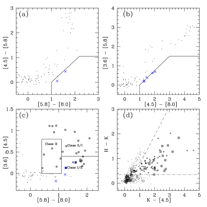
Figure 7: (a) & (b). IRAC CC diagrams to identify star-forming galaxies, using the method described in Gutermuth et al. (2008). The zones where these extragalactic sources are located in the CC diagrams are marked with solid lines. (c). IRAC CC diagram to identify YSOs. The different zones indicate the locations of Class II, Class I and Class 0 sources from Allen et al. (2004). (d). The $H-K$/$K-[4.5]$ CC diagram. The curved line is the MS locus of late M type dwarfs (Patten et al. 2006). The long-dashed line corresponds to the reddening vector (from Flaherty et al. 2007). The dashed-dotted horizontal line represents the $H-K$ color cut off for the selection of YSOs (see the text).

The circumstellar disk emission dominates at longer wavelengths, where the spectral energy distribution (SED) significantly deviates from the pure photospheric emission. Hence, the IRAC bands can be used to identify IR-excess emission sources (cf. Allen et al. 2004, Megeath et al. 2004). However, contamination from extragalactic sources such as polycyclic aromatic hydrocarbons (PAH)-rich star-forming galaxies and AGNs, limit the use of this method as both types of sources display colors similar to that of YSOs. Various authors have investigated the contamination of AGNs and galaxies in the IRAC CC diagrams. We followed the approach of Gutermuth et al. (2008) and Stern et al. (2005) to identify galaxies and AGNs in IRAC CC diagrams. The zones identified by Gutermuth et al. (2008) in [3.6]-[5.8]/[4.5]-[5.8] and [4.5]-[5.8]/[5.8]-[8.0] CC diagrams for PAH-rich star-forming galaxies are marked by solid lines in Figs. 7$a$ and 7$b$, where small dots represent the sources identified in all the four IRAC bands within a $\sim$ 8^′$\times$ 8^′ region, covering the FOV of our NIR observations. The sources marked as crosses in Figs. 7$a$ and 7$b$ are star-forming galaxies. Stern et al. (2005) found broad-line AGNs in a specific zone in the [3.6]-[4.5]/[5.8]-[8.0] CC diagram using optical spectroscopic observations, however this zone is also occupied by protostars (Allen et al. 2004). Similarly, in a nearby star-forming region, Fazio et al. (2004b) found that 50% of the sources with [3.6] $>$ 14.5 mag are extragalactic in nature. Since our star-forming region is at a farther distance, some of the YSOs in our sample may appear fainter than 14.5 mag in the IRAC 3.6 $\mu$m band. Our search of AGNs by combining both the methods as mentioned above, results no contamination of AGNs in our sample of YSOs. After identifying the extragalactic contamination we used IRAC [5.8]-[8.0]/[3.6]-[4.5] CC diagram, shown in Fig. 7$c$ to identify the IR-excess sources (i.e., YSOs). In the CC diagram, the regions occupied by Class II, Class I/II and Class 0/I objects are indicated following the classification scheme by Allen et al. (2004). However, as noted by Whitney et al. (2003b), the SEDs of highly inclined Class II sources closely resemble the SEDs, and therefore, the colors of Class I sources (Whitney et al. 2003b; Allen et al. 2004). These facts make the boundary between Class I and Class II sources somewhat indistinct and also Class II objects hidden behind large quantity of dust can also be shifted to Class I zone. Here, all the sources with [5.8]-[8.0] $\geq$ 0.4 and [3.6]-[4.5] $\geq$ 0.1 are assumed to be probable YSOs after eliminating star-forming galaxies. On the basis of the above criteria, the [5.8]-[8.0]/[3.6]-[4.5] CC diagram yields 27 YSOs, which are marked as squares in Fig. 7$c$. The search of YSOs on the basis of [5.8]-[8.0]/[3.6]-[4.5] CC diagram could be affected by the lower sensitivity of IRAC 5.8 and 8.0 $\mu$m bands to detect faint sources. As 4.5 $\mu$m emission traces hot circumstellar dust and is less affected by PAHs, we used a combination of $H$, $K$, and IRAC 4.5 $\mu$m bands to detect IR-excess sources. Fig. 7$d$ shows the $H-K$/$K-[4.5]$ CC diagram. The solid curve in the diagram represents the locus of MS late dwarfs (Patten et al. 2006) and the dashed line denotes the reddening vector from the tip of M6 dwarf, using the average extinction law by Flaherty et al. (2007). The stars with IR-excess are located to the right of the reddening vector and are marked as circles. The squares represent the YSOs selected from the IRAC [5.8]-[8.0]/[3.6]-[4.5] CC diagram. Since most of the field stars in the $K$/$H-K$ CM diagram (see Fig. 6$b$) have colors $H-K$ $\leq$ 0.35, we therefore adopted a conservative approach to select IR-excess sources in Fig. 7$d$ by considering sources having $H-K$ $\geq$ 0.35 and which are also lie to the right of the reddening vector. As can be seen in Fig. 7$d$ the majority of the YSOs selected on the basis of Fig. 7$c$ fall above these color cutoffs.

Combining IRAC photometry with NIR observations, we find a total of 150 likely YSO candidates with circumstellar disks, that include Class I and Class II sources, which indicate a site of active star formation. The spatial distributions of these YSO candidates are used to study the star formation scenario in this complex, along with their correlation to the associated gas and dust (see §7.2).

5.4 Ionized gas distribution

There are several radio interferometric studies, mainly towards the regions A, B, C and D in the frequency range of 5-15 GHz (Harris 1975; Kurtz et al. 1994; DePree et al. 1994) with resolutions better than 3^′′.5, available in the literature. Our radio continuum maps at 610 MHz & 1280 MHz are shown in Figs. 4 and 5, with a resolution of 5^′′.5 $\times$ 4^′′.8 and 3^′′.3 $\times$ 3^′′.0, respectively. To our knowledge these observations are the highest angular resolution images at low frequency to date. The 1280 MHz map shows the radio emission from the five components A, B, C1, C2 and D. The components C1 and C2 are embedded in an envelope of more diffuse emission, whereas the component A shows extended emission in northwest and southwest directions. The extended emission in the southwest appears to connect to the low brightness emission seen to the north of K3-50D. The measured peak position, integrated flux density and angular diameter, deconvolved from the beam for roughly spherical compact sources A, C2 and C1, were determined by fitting a two-dimensional elliptical Gaussian using the task JMFIT in AIPS. For irregular, diffuse extended sources D and B, these observed parameters were obtained using the task TVSTAT in AIPS. The flux densities and dimensions for these extended sources were obtained by integrating over the approximate angular size of the contour map above 3$\sigma$ (where $\sigma$ is the rms noise in the map). These observed estimations are given in Table 3. An error of 10-15 $\%$ is expected to be associated with these values due to the combination of the rms noise in the map ($\sigma$), the flux calibration error (within 7%) associated with source flux (S) and the uncertainty in flux extraction of the source ($\sigma_{\rm{source}}$). The combined error is estimated as; $\sigma_{\rm{S}}$ = $\sqrt{{\sigma}^{2}+(0.07S)^{2}+\sigma^{2}_{\rm{source}}}$. Here, we expected a negligible amount of the missing flux from the compact sources, however in the case of extended sources, the uncertainty in the flux estimation could be high, hence the quoted error for such sources should be considered as a conservative lower limit. The integrated flux and size of the cores of C1 and C2 should be considered as an upper limit, since the cores are embedded in an envelope of diffuse emission and the present angular resolution is insufficient to resolve C1 and C2. It is not known whether the extended emissions of the envelopes are either ionized by the sources in the cores and/or (partly) by the nearby external source. The radial velocity of the extended emissions and the compact cores are required to know their physical association. The images show that all the sources have complicated morphology. The determination of important physical parameters is hampered due to the complicated morphology of the sources because these parameters, such as density and surface brightness along the line of sight, depend on the source structure. In the present study, we calculate the physical parameters assuming the simplest geometry of uniform spherical model. The physical parameters are such as: $n_{e}$, the rms electron density; EM, the emission measure; $\tau$_c, the optical depth; $N_{Lyc}$, the number of Lyman continuum photons for a spherically symmetric region; and the spectral type of the ionizing source, assuming a single ZAMS star from the $N_{Lyc}$. These parameters were derived from the measured angular diameter and integrated flux density using the formulae given by Panagia & Walmsley (1978) and Mezger & Henderson (1967) for spherical, homogeneous nebulae. We have assumed an electron temperature of 10⁴ K and source size as the geometrical average of the major and minor axes, as listed in Table 3, to derive the physical parameters. The derived physical parameters are listed in Table 4. However, the uncertainties are associated with the values given in Table 4 because of our limited knowledge of the source structures, dust absorption of Lyc photons (Garay et al. 1993) at low frequency for CH ii and UCH ii regions (e.g., K3-50A & K3-50C) and missing flux from the low density components (e.g., K3-50D & K3-50B). As the gas seems to be clumpy in nature, the rms electron density of the regions is expected to be lower than the density at the peak positions. The sources K3-50C1 and K3-50A are optically thick at 1280 MHz, therefore the spectral type, electron density derived by this method should be considered as the lower limit. The spectral types of the ionizing sources for the components K3-50B and K3-50D may be earlier than the present estimation possibly due to missing flux from the low density components. The spectral types suggest that all the sources are ionized by massive late O-type ZAMS stars and their physical parameters point to a different evolutionary class of regions (Kurtz et al. 2000).

5.5 Candidates for the ionizing sources of the regions

The OB type stars associated with K3-50 region are significantly contaminated by the luminous field stars (see §5.1). Therefore, in order to identify the probable ionizing candidates of the individual regions, we used our $JHK_{\rm s}$ catalogue. We searched for ionizing sources in a circular area of radius $\sim$ 0.5 pc from their radio-emission peak, except for the source K3-50D which shows core-halo morphology (see §6.1). We identified the ionizing source of K3-50D using optical spectroscopy and discussed in section 6.1. The probable sources are shown in $(J-H)$ versus $(H-K)$ CC diagram (Fig. 8$a$) as well as in $(J-H)$ versus $J$ CM diagram (Fig. 8$b$). Fig. 9 shows $K_{\rm s}$-band image with the sources located within the radius $\sim$ 0.5 pc of each region, along with the ionizing source of K3-50D. The sources are labeled with numbers corresponding to the regions. In Fig. 8$a$, sources (A1, A2, C2 and F2) show NIR excess. Therefore, the spectral type estimation on the basis of $(J-H)$ versus $J$ CM diagram should be considered as an upper limit for these sources. In order to distinguish the Galactic field stars from the OB stars, we further constrain our analysis by using a reddening-free quantity Q = $(J-H)$ - 1.70 $(H-\mbox{$K_{\rm s}$~{}})$, which is $\sim$ 0 for early type stars with no NIR excess and $\sim$ 0.4-0.5 for Galactic field stars and negative for NIR excess sources (Comerón & Pasquali 2005). As the sources (A1, A2, C2 and F2) show considerable NIR excess and may be the candidates for ionizing sources, we selected the sources with Q value $<$ 0.3 as possible ionizing sources. It is worthwhile to point out that the sample identified using the criterian Q $<$ 0.3 may also be contaminated by objects such as; AGB stars, carbon stars, foreground F-type stars and background A-type giants (Comerón & Pasquali 2005). Since we are looking for early type stars within the radio emitting region in a circular area of radius $\sim$ 0.5 pc around the radio emission peak, we presume the probability of contamination is less, however this can not be ruled out. Moreover, in $(J-H)$ versus $J$ CM diagram, we selected luminous sources that have spectral type earlier than B3, which further reduces the possibility of contamination. The estimated photometric spectral types for the probable ionizing sources (details are discussed in their individual sections) with Q $<$ 0.3 along with the spectral type estimated from radio observations at frequencies in which these regions are optically thin, are mentioned in Table 5. Here, it is noted that the ZAMS spectral types given in Table 5 are taken from Panagia (1973), corresponding to the $N_{Lyc}$ photons s^-1 reported by DePree et al. (1994) from 14.7 GHz observations. It is evident from Table 5 that all the regions are excited by early-B to late-O type of stars, which confirms the estimation by radio observations, except the source A (see §6.2 for further discussion on source A).

6 Nature of Individual Sources

6.1 K3-50D

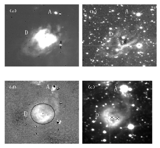
Figure 10: Images of K3-50D and K3-50A (clockwise from the top left panel) : (a) The continuum-subtracted image of H$\alpha$ (6563 Å) + [N ii] (6548 Å  and 6584 Å), (b) Bias and flat-field corrected image of [S ii] at 6717Å+ 6731 Å  (c) IRSF $K_{\rm s}$-band image with two bright sources (marked with crosses) inside the semi-circular shell (d) Continuum-subtracted Br$\gamma$ image, marked with a circle of $\sim$ 50^′′ radius around central bright star.

The morphological features of the nebula at different optical and NIR bands are shown in Fig. 10. The ionized gas is seen in H$\alpha$ with an extended ring, whereas [S ii] image shows a limb brightened shell towards the western side. The Br$\gamma$ image traces a semi-circular shell of ionized gas with the shell opening towards the north-western side. The same morphology is also seen in IRSF $K_{\rm s}$-band image. In the IRSF $K_{\rm s}$-band image, two bright sources are visible within the ring of ionized gas. The star situated at the center of nebula is the main ionizing source of ZAMS spectral type $\sim$ O5 (§5.5), whereas the colors ($J-H$ $\approx$  0.32, $H-K$ $\approx$  0.20) of the second source situated at 12^′′ towards the south-western direction from the central star suggest a reddened giant, which is supported by its $Q$ value of $\sim$ 0.38. A plausible model for this type of morphology could be the displacement and ionization of the gas due to the stellar wind produced by the massive star at the center of the nebula. The one-dimensional spectrum of the star in the range 3950-4750 Å is shown in Fig. 11$a$. We classified the spectrum by comparing the observed spectrum with those given by Walborn & Fitzpatrick (1990). Besides hydrogen Balmer lines (H_γ, H_δ, H_ϵ, etc), the spectrum displays prominent He ii line at $\lambda$ 4200 Å, and strong He ii line at $\lambda$ 4686 Å. These features indicate that the star should be an O-type of luminosity class V. In the case of O-type stars the classification of different subclasses are based on the strengths of the He ii lines at $\lambda$ 4541 Å  and $\lambda$ 4471 Å. The equal strength of the lines implies a spectral type of O7, whereas the greater the strength of $\lambda$ 4541 Å  He ii line as compared to $\lambda$ 4471 Å  line implies a spectral type earlier than O7. If the strength of He i + He ii $\lambda$ 4026 Å  $\leq$ $\lambda$ 4200 Å  He ii , it favors classification earlier than $\sim$ O5.5. Comparing the strengths of these lines we adopt the classification as $\sim$ O4V, which is in agreement with the estimation by Georgelin (1975). Roelfsema et al. (1988) estimated a visual extinction of 2 mag towards K3-50D from the ratio of expected Br$\alpha$ emission predicted from radio emissions to the observed Br$\alpha$ emission, whereas Persson & Frogel (1974) estimated a visual extinction of $\sim$ 4.4 mag using the spectrophotometric measurements of hydrogen lines of the nebula associated with the K3-50D. To estimate the extinction towards the region, we use the $(U-B)/(B-V)$ CC diagram. Morphologically K3-50D shows a bright star at the center and a partial ring of ionized gas of diameter $\sim$ 40^′′, therefore we restrict our optical analysis within a circular area of diameter $\sim$ 50^′′ to avoid field star contamination. The $(U-B)$ versus $(B-V)$ CC diagram of the region is shown in Fig. 11$b$. To match the observations, the ZAMS by Schmidt-Kaler (1982) is shifted along the reddening vector having a normal slope of $\frac{E(U-B)}{E(B-V)}=0.72$. The CC diagram indicates a minimum reddening of $E(B-V)_{min}$ = 1.36 mag for the stars within $\sim$ 50^′′ region. Using the relation $A_{\rm V}$ = 3.1 $\times$ $E(B-V)$, the estimated value of $A_{\rm V}$ comes out to be $\approx$  4.2 mag. We also estimated the average visual extinction for the region, using stars with spectral type earlier than A0 by ‘Q’ method (Johnson & Morgan 1953). The intrinsic colors of these stars were obtained from the relation $(B-V)_{0}$ = 0.332 $\times$ Q (Hillenbrand et al. 1993). To check the bias of the contamination of other field sources to this value, we estimated the visual extinction from the ionizing source of K3-50D. The O-type MS star shows a narrow range in their intrinsic colors. Adopting an intrinsic color $(B-V)_{0}$ = -0.33 (Cox 2000) for the ionizing star of K3-50D and using the measured photometric color $(B-V)$ = 1.04, we derived an excess $E(B-V)$ = 1.37, which in turn gives $A_{\rm V}$ $\approx$ 4.2 mag, which agrees well with the estimation based on the CC diagram. Since the distance estimates to the region are uncertain and vary from 4.5 to 12.5 kpc (Israel 1976), the present spectral classification of the ionizing star and reliable estimation of extinction together with the present apparent magnitude of the ionizing source enables us to derive its distance. Using the present spectral classification (O4V) along with $A_{\rm V}$ $\approx$ 4.2 mag, V = 13.31 and $M_{\rm V}$ -spectral type calibration table of Vacca et al. (1996), we estimated a distance of $\sim$ 8.5 kpc for the K3-50D region. However, the spectroscopic distance determination is strongly dependent on the assumed value of $M_{\rm V}$ and the values of $M_{\rm V}$ in case of O4V star vary from -5.4 (Schmidt-Kaler 1982) to -5.9 (Conti 1988) in the literature, which in turn can vary distance from 7.9 kpc to 10 kpc. However, recent investigation by Martins et al. (2005) found considerable shift in calibration of effective temperature in early type stars. The $M_{\rm V}$ value of O4V star ($M_{\rm V}$ = -5.5) by Martins et al. (2005) results in a distance of 8.6 kpc to the region. These estimations are consistent with the average kinematic distance ($\sim$ 8.7 kpc) towards K3-50 and supports its association with the W58 molecular cloud.

6.2 K3-50A

K3-50A is a CH ii region, ionized by a single O5.5V star and its angular size is $\sim$ 4^′′.1 $\times$ 3^′′.4 at 14.7 GHz (Kurtz et al. 1994). The radio continuum peak is coincident with 10 $\mu$m peak, whereas the associated optical emission (see §1) is located to the south-west ($\sim$ 2.5^′′) of the radio peak (Wynn-Williams et al. 1977) and the region is possibly ionized by multiple sources (Okamoto et al. 2003). We detected two NIR sources in all the three bands within $\sim$ 0.5 pc radius of the radio peak. The source A1 shows a large IR-excess ($H-K$ $\approx$  3.35) and is also more luminous ($K$ $\approx$  9.11) than any reddened O-type stars of the complex. The second bright source A2 is located outside the radio size ($\sim$ 4^′′) of K3-50A, hence the probability of this source as one of the ionizing candidates is rather low. Therefore, A1 is the most probable ionizing source of K3-50A. We speculate that all the point sources close to the nebula (e.g., A2) may be strongly contaminated by the intense $K_{\rm s}$-band nebulosity of K3-50A. The crowding in the region has already been noticed by Okamoto et al. (2003), therefore, the spectral classification on the basis of NIR photometry may be affected by source contamination along with bright nebulosity and will yield an earlier spectral type.

6.2.1 Spectrum of the Nebula

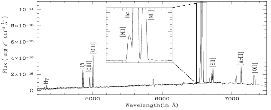
Figure 12: The observed flux-calibrated optical spectrum of the compact nebula associated with K3-50A.

Fig. 10$a$ shows the continuum-subtracted H$\alpha$ + [N ii]  image of the optical nebula associated with K3-50A. The spectrum of the nebula is presented in Fig. 12. The nebula shows forbidden emission lines as seen in the case of regions. We obtained the emission line fluxes by Gaussian fitting of the line profiles and by direct integration of the fluxes over the local continuum with SPLOT routine of the IRAF package. Uncertainties in these line intensities depend upon the strength of the lines and blending with adjacent lines. The measurement errors for the isolated bright lines (fluxes larger than $\sim$ 10^-14 ergs cm^-2 s^-1) are expected to be less than 10%, whereas for the weaker and blended lines like H$\alpha$ + [N ii]  and [S ii], the measurement uncertainties can be as large as 20%. Our measurements are consistent with that of Persson & Frogel (1974) for the common lines.

The physical parameters of the nebula can be derived from the diagnostic of line ratios with certain assumptions. Since our spectrum contains emission lines of hydrogen, their relative intensities can be used to estimate the reddening for the region. We obtained the reddening coefficient C($H_{\beta}$) $\approx$ 3.16, by comparing the observed ratio of H$\alpha$/H_β with the theoretical ones calculated by Osterbrock (1989), for the temperature 10⁴ K and density 10⁴ cm^-3, using Case-B recombination theory and extinction law of Cardelli, Clayton & Mathis (1989, hereafter CCM 89). Here, we would like to mention that the presence of extinction increases with the observed ratio, because extinction affects the H_β wavelength more than the H$\alpha$ wavelength and also the ratio depends on the geometry of the dust and gas cloud. However, Persson & Frogel (1974) found variable extinction within the region by comparing the radio, infrared and optical emission fluxes. Wynn-Williams et al. (1977) found that these emissions are not coincident and the location of peak intensity moves from the radio center towards the southwest direction as the wavelength decreases. The position of the optically visible nebula is approximately 2^′′.5 away from the peak of radio position. On the basis of a deep 9.7 $\mu$m absorption feature in the MIR spectra, it is interpreted that K3-50A is partly obscured by a dense dust cloud (Thronson & Harper 1979 and references therein), which supports similar conclusion of Wynn-Williams et al. (1977). To explain the strong extinction gradient across the region, Wynn-Williams et al. (1977) proposed a possible geometry that the K3-50A is a partially ionization bounded CH ii region formed near the edge of an obscuring cloud and is now eating its way to the less dense region at the edge, like the Orion Nebula region.

Assuming that the optical lines represent the physical properties of local environment, we retain our analysis with $A_{\rm V}$ $\sim$ 6.79 mag, which has been derived using the extinction law $A_{\rm V}$ $\sim$ 2.145 $\times$ C($H_{\beta}$) (CCM 89). All the line fluxes were dereddened using $A_{\rm V}$ $\sim$ 6.79 mag and extinction law of CCM 89. Table 6 lists the observed and reddening corrected emission line intensities relative to H_β. We estimate the electron density $\sim$ 0.67 $\times$ 10⁴ cm^-3 using 5-level atom program by Shaw & Dufour (1994) from the [S ii] ($\lambda$ 6717 / $\lambda$ 6731) line ratios, assuming $T_{e}$ = 10⁴ K. This assumption is not critical because the density calculated from [S ii] lines are nearly independent of $T_{e}$. The [S ii] line ratio ($\sim$ 0.54) lies close to the high density limit, probably due to the collisional quenching of forbidden lines, hence the estimated electron density should be considered as a conservative lower limit though it might be higher. It is noted that the density derived from the [S ii] lines is representative of a nebula $\sim$ 2^′′.5 away from the high-density core, traced by high frequency high resolution radio observations. Therefore, the electron density estimated with high frequency radio observations is expected to be higher than density from [S ii] lines. We estimate the electron temperature $T_{e}$ ([N ii] ) from the temperature sensitive intrinsic [N ii] (6548 Å+ 6583 Å/ 5755 Å) line intensity ratio, which turns out to be $\sim$ 10496 K. However, it should be noted that 5755 Å  line is quite faint as seen in the spectrum. A roughly linear, increasing trend in [O III] (4959 Å+ 5007 Å)/$H_{\beta}$ with stellar temperature is expected, because the nebular volume containing doubly ionized oxygen increases with the higher ionizing flux emitted by early spectral type stars. By comparing the [O III] (4959 Å+ 5007 Å)/$H_{\beta}$ value $\sim$ 1.79 of K3-50A, with that of values in the range 1.71 to 1.86 for the Galactic regions ionized by a single star (Kennicutt et al. 2000), a rough estimation of stellar temperature of the ionizing star hotter than 35900 K and cooler than 42700 K can be obtained. Thus, from the stellar temperature, a MS spectral type between O9 to O6.5 (Vacca et al. 1996) is expected as the probable exciting source of the nebula.

6.2.2 Sub-millimeter emission from cold dust

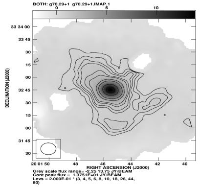
Figure 13: Contour map of spatial distribution of cold dust emission at 850 $\mu$m around K3-50A region. The contour levels are drawn above 3$\sigma$, where $\sigma$ is the rms noise ($\sim$ 2 mJy) in the map and the FWHM of the symmetric 2-D Gaussian beam is $\rm 14\arcsec.0$. The labelled axes are in J2000 coordinates.

As star-forming regions are optically thin for wavelengths longer than $\sim$ 200 $\mu$m, thermal dust emission can be used to determine the physical parameters such as mass and density of star-forming regions. Continuum sub-millimeter fluxes at 850 $\mu$m and 450 $\mu$m for the K3-50A were obtained from Thompson et al. (2006). The integrated flux densities at 450 $\mu$m and 850 $\mu$m are 256 $\pm$ 79.3 Jy and 37 $\pm$ 4.3 Jy, respectively. The peak flux densities are 53.6 $\pm$ 16.1 Jy/beam and 13.6 $\pm$ 1.4 Jy/beam at 450 and 850 $\mu$m, respectively. The 850 $\mu$m map is shown in Fig. 13. The bright continuum emission is concentrated towards the central region of K3-50A, showing a core peaking at $\alpha_{2000}=20^{h}01^{m}45^{s}$, $\delta_{2000}=+33^{\circ}32^{\prime}44^{\prime\prime}$, with extended emission along the northeast and southwest directions. For optically thin emission, the dust mass can be estimated from the standard method of Hildebrand (1983) and the total mass (dust plus gas) of the cloud is given by

$$M=\frac{d^{2}F_{\nu}C_{\nu}}{B_{\nu}(T_{\rm d})},$$ (1)

Where $F_{\nu}$ is the flux density at frequency $\nu$, $B_{\nu}(T_{\rm d})$ is the Planck function evaluated at frequency $\nu$ and dust temperature $T_{\rm d}$. The parameter $C_{\nu}$ is a mass conversion factor combining both the dust-to-gas ratio and the frequency-dependent dust opacity $\kappa_{\nu}$ and $d$ is the distance to the source in kpc. Various values for $C_{\nu}$ are quoted in the literature; here we have adopted a value for $C_{\nu}$ of 50 g  cm^-2 at 850 $\mu$m, following the method of Kerton et al. (2001), which is appropriate for dense molecular cores. The integrated flux over the region at 850 $\mu$m gives the mass of the cloud as $\sim$ 7800 $M_{\odot}$ for an assumed average dust temperature of 30 K for the entire cloud. The main error in this estimate is likely due to the uncertainty in the dust temperature. Because of non-linear dependence of the Planck function on temperature, a small change in temperature leads to a large change in the calculated dust mass (e.g., a 5 K error in temperature leads to an error of $\sim$ 40% in mass estimation). Hence we consider the present mass estimate from the dust emission to be accurate only within an order of magnitude.

6.2.3 Spectral Energy Distribution

The star A1 shows large infrared excess (Fig. 8$a$) and is located close to the peak of the molecular core having weak bipolar outflow (Phillips & Mampaso 1991), a phenomenon that is thought to be closely related to the accretion process. Molecular outflows are common phenomenon in the early stage of massive star formation prior to formation of UCH ii region (e.g., Beuther et al. 2002) and also during the UCH ii phase (e.g., Shepherd & Churchwell 1996). To investigate the nature of A1, we constructed SED using the recently available grid of models and fitting tools of Robitaille et al. (2006, 2007). The models are computed using a Monte-Carlo based radiation transfer code (Whitney et al. 2003a, b), using several combinations of central star, disk, in-falling envelope and bipolar cavity, for a reasonably large parameter space. To produce the observed SED, we have used the data from the following: 1.25-2.17 $\mu$m (Alvarez et al. 2004), 3.5 and 10.1 $\mu$m (Neugebaure & Garmire 1970); 8-21 $\mu$m, MSX PSC (Egan et al. 2003); 450 and 850 $\mu$m (Thompson et al. 2006). The SED is shown in Fig. 14. Here, we would like to mention that the angular resolutions for most of the data are not sufficient to derive precise parameters for a single YSO. We set MSX and sub-mm fluxes as upper limits to account for possible contribution from other sources that might be included within the large beam of the observations. We further set 20 to 10$\%$ error in NIR and MIR flux estimates due to possible uncertainties in the calibration, the extinction and intrinsic object variability. A distance range of 7 to 10 kpc and the visual extinction in the range from 15 to 30 mag are used as input parameters to the model to construct the SEDs. The parameters obtained from the weighted mean and standard deviation of all the models with ${\chi}^{2}-{\chi_{best}}^{2}<3$ (per data point), weighted by inverse square of ${\chi}^{2}$ of each model, suggest the associated source is a massive YSO with mass $M_{\star}$ = 42 $\pm$ 4.4 $M_{\odot}$ and of total luminosity Log($L_{\star}$) = 5.6 $\pm$ 0.2 $L_{\odot}$. The models also predict that the source is deeply embedded behind 17.5 $\pm$ 1.8 mag of visual extinction and has an envelope accretion rate of Log($\dot{M}_{env}$) = -3.8$\pm$ 0.2 $M_{\odot}$ yr^-1 with no disk. The SEDs of high mass protostars are dominated by the envelope flux, where the disk flux is almost embedded within the envelope flux. Therefore, the models with envelopes alone and the models with disks and envelopes successfully fit the same SED (Grave & Kumar 2009). It is to be noted that these models are valid for isolated objects. Therefore, considering the presence of multiple point sources claimed by Okamoto et al. (2003), the above parameters should be taken with caution. Nevertheless these models provide quantitative information about the nature of the object.

6.3 K3-50B

The $K_{\rm s}$-band image of K3-50B shows unusual distribution of dust within the region with an elongated hole from east to west (see Fig. 3). The morphology of 610 MHz map (Fig. 4) suggests a blister type region, where a sharp ionization bounded edge can be seen towards the western direction. Towards the east, the gradient of flux density indicates a density-bounded side of the blister morphology. The high resolution image at 1280 MHz (see Fig. 5) also shows non-uniform clumpy distribution of ionized gas. The complex structure of radio emission suggests that it may have been produced through excitation by multiple stars (e.g., Ojha et al. 2004a; Garay et al. 1993) or presence of density inhomogeneities within the region excited by a single luminous star. We detect four sources (marked in Fig. 9) within a radius of $\sim$ 0.5 pc from the center of the nebula. The source B4 is a bright infrared source ($K$ $\approx$  11.27, $H-K$ $\approx$  0.88) with $Q$ $\approx$  0.06, whereas the source B3 ($K$ $\approx$  12.47, $H-K$ = 0.31) has $Q$ $\approx$  0.31. The source B3 is bright in the optical wavelengths and being situated at the central region of the nebula gives an impression of it being one of the ionizing candidates. The optical spectrum of the source B3 in the range 3950-4750 Å  is shown in Fig. 15. Due to low S/N ratio, the exact spectral classification of the source is rather difficult, but the absence of absorption lines (He ii at $\lambda$ 4200 & $\lambda$ 4686 Å, He i at $\lambda$ 4026 & $\lambda$ 4471 Å, Si ii at $\lambda$ 4128 & $\lambda$ 4130 Å  and Mg ii at $\lambda$ 4481 Å), suggest that source B3 is not an OB-type star. The source B1 has $Q$ $\approx$  0.49, along with $H-K$ $\approx$  0.61, which suggests a reddened giant rather than a ZAMS star. The positions of the sources B1 and B3 on the CC diagram (Fig. 8$a$) fall close to the giant locus, confirming the above argument. The source B2 with $Q$ $\sim$ 0.12, indicates that it could be one of the ionizing candidates of ZAMS spectral type of B2-B3, but its low visual extinction ($A_{\rm V}$ $\approx$  3.8 mag) in comparison to $A_{\rm V}$ $\approx$ 26 mag (Roelfsema et al. 1988) towards K3-50B suggests a field star. The source B2 seems to have spectral type later than B2. As the star of spectral type later than B2V emits $<$ 2 $\%$ of its total output energy in terms Lyc photons per second, therefore the source B2 cannot be one of the main ionizing candidates of K3-50B. The position of the source B4 on NIR CM diagram (Fig. 8$b$) shows the characteristics of ZAMS spectral type $\sim$ O5, which is consistent with spectral type ($\sim$ O6-O5.5) derived from Lyc fluxes from radio observations, therefore B4 can be the most probable ionizing candidate for K3-50B. The spectral type estimation of B4 is not biased by excess emission as it does not possess NIR excess, therefore the complex structures of the K3-50B region are probably due to density inhomogeneities rather than due to multiple early-type sources in the region.

6.4 K3-50C

K3-50C is located $\sim$ 2^′.5 northeast from K3-50A and consists of two radio continuum sources C1 and C2. These sources are separated by $\sim$ 15^′′ and C1 is stronger than C2 at 8.4 GHz (Kurtz et al. 1994) and 15 GHz (DePree et al. 1994) radio wavelengths. However, below 20 $\mu$m C2 is much stronger than C1 and C1 is barely detected at 20 $\mu$m and is not seen at shorter wavelengths (Wynn-Williams et al. 1977), indicating that C1 is more deeply embedded in molecular cloud of high visual extinction as compared to C2. C2 is located at the center of a prominent $K_{\rm s}$-band nebulosity in K3-50C region, where we detect a bright NIR point source close to the radio peak. The positions of the source C2 on CC and CM diagrams (Figs. 8$a$ & 8$b$) indicate a reddened ZAMS spectral type between B0 - O9.5 with NIR excess. The NIR spectral type estimation agrees well with the $\sim$ O9 ZAMS spectral type derived from radio continuum observations. The position of C1 falls on the dark lane that bisects $K_{\rm s}$-band diffuse emission into north and south components (Fig. 3). A large variation of extinction is found in the direction of C1. At the peak of radio continuum emission no Br$\alpha$ was detected, indicating a visual extinction of $\geq$ 190 mag (Roelfsema et al. 1988), which is the possible cause for the non-detection of ionizing source(s) in our infrared survey around the radio peak. The N_Lyc photons s^-1 from the region suggest that C1 is ionized by a single O8-O9 ZAMS star. The spectral type estimation on the basis of radio continuum photons is an indirect approach in the absence of estimation based on direct stellar radiation from the star(s). Therefore, here the possibility that more than one star might be responsible for the ionization of C1 cannot be excluded, since massive star formation usually proceeds in cluster mode. In this case, the spectral type of the most luminous star must be later type than that derived from the single-star hypothesis.

6.5 K3-50E and K3-50F

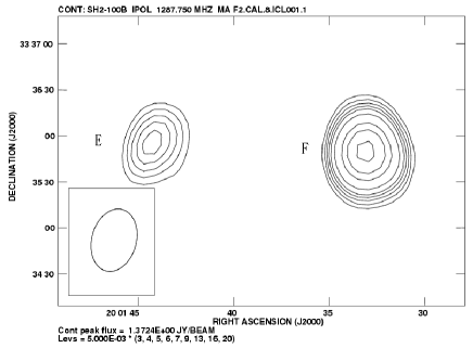
Figure 16: Low resolution ($\sim$ $\rm 44\arcsec\times 27\arcsec$) radio continuum map at 1280 MHz for the regions K3-50E and K3-50F. The contour levels are at 5.0 $\times$ (3, 4, 5, 6, 7, 9, 13, 16, 20) mJy/beam, where $\sim$ 5.0 mJy/beam is the rms noise in the map. The labelled axes are in J2000 coordinates.

K3-50E and K3-50F are two faint optical nebulosities separated by 2′.2 (Fig. 1). Our low resolution ($\sim$ 44^′′ $\times$ 27^′′) map at 1280 MHz (see Fig. 16) shows continuum emission from ionized gas around both the regions, with K3-50F being relatively brighter than K3-50E. In Fig. 4, bright $K_{\rm s}$-band sources can be seen within the radio contours, which are also visible in the optical (K3-50E: $V$ = 17.16, $B-V$ = 1.543; K3-50F: $V$ = 14.95, $B-V$ = 1.282). These sources are located within the radius of $\sim$ 0.5 pc from the radio peak, and so are most likely the ionizing sources of the nebulae. Their visual extinctions estimated using the ‘Q’ method (§6.1) suggest that they are extincted by visual extinction of 5.6 and 4.8 mag, respectively.

There are no definite estimations of distance for K3-50E and K3-50F in the literature but they are assumed as $\sim$ 8.7 kpc (Israel 1976). Hence, to estimate approximate distance we use the following relation given by Comerón & Torra (2001) for an ionization bounded optically thin region with an electron temperature of $\sim$ 10⁴ K :

$$D(kpc)\approx 5.35\times 10^{-3}[\frac{\nu^{0.1}(GHz)S_{\nu}(J_{y})}{\Sigma^{N}_{i=1}10^{-1.26H_{oi}}}]^{0.233}$$ (2)

where S_ν is the flux density in Jy at frequency $\nu$ (in GHz). $H_{oi}$ is the dereddened $H$-band magnitude of ‘i’ th ionizing star. Due to the small sizes of both the regions and our selection method to identify possible ionizing sources described in section 5.5, we believe that the two optically bright sources are most likely the ionizing sources of the regions. Using the above approximate relation, we obtain distances of $\sim$ 7.6 kpc and $\sim$ 8.4 kpc for K3-50E and K3-50F, respectively. Here, we assume that both the regions are ionization bounded and ionized by a single star. In Eq. 2 we have used radio fluxes ($\approx$  0.04 Jy for K3-50E and $\approx$  0.13 Jy for K3-50F) estimated from the low resolution map (Fig. 16), the $H$-band magnitudes ($\approx$  12.75 mag for K3-50E and $\approx$  12.25 mag for K3-50F) of the ionizing stars and extinction at $H$-band ($\approx$  0.87 mag for K3-50E and $\approx$  0.74 mag for K3-50F). Although the above approximate distance estimates agree with the kinematic distance (7.9 to 9.3 kpc) reported towards the direction of K3-50 SFR, the validity of the method is constrained by the number of assumptions concerning membership, dereddening, dust absorption of Lyc photons, leakage of ionizing photons from the regions and uncertainty in the radio flux estimations. The more precise distance can be estimated using observed photometric magnitudes and accurate spectral type of the ionizing sources as described in section 6.1 for K3-50D. We estimated Lyc photons per second from the integrated fluxes at an assumed distance of 8.7 kpc and that come out to be $\sim$ 1.5 $\times$ 10⁴⁷ s^-1 and $\sim$ 4.8 $\times$ 10⁴⁷ s^-1 for the K3-50E and K3-50F, respectively. These fluxes correspond to ZAMS spectral types of B0.5-B0 and B0-O9.5, respectively, consistent with the ZAMS spectral types estimated from $J-H$ versus $J$ CM diagram (see Fig. 8$b$ and Table 5).

7 General discussion

7.1 Extinction towards individual regions

The massive stars (M $>$ 8$M_{\odot}$) do not have pre-main-sequence (PMS) phase and the object reaches ZAMS while still embedded in the molecular cloud (Palla & Stahler 1990). We used probable ionizing sources (see Table 5) of the individual regions to derive their extinction values. We traced the ionizing stars back to their intrinsic ZAMS position in $(J-H)$ versus $J$ CM diagram (Fig. 8$b$) along the reddening vector. However, the uncertainty in estimation of extinction cannot be ruled out due to excess emission in $J$ and $H$ bands. This could be the case for the ionizing star A1 of K3-50A region, which shows maximum NIR excess among all the YSOs. The visual extinction toward regions A, B, C2, D, E and F is estimated to be 31.2, 16.1, 21.2, 4.4, 5.9 and 5.5 mag, respectively. Here it is to be noted that the extinction estimates for A1 and C2 must be towards the higher side as these stars have significant NIR excess. For example, in the case of A1, the extinction value derived from the SED fitting (§6.2.3) comes out to be 17.5 $\pm$ 1.8 mag. The above discussion along with the average extinction found towards C1 (see §1) indicate that the K3-50 SFR shows variable extinction in the range of 4.4 - 97 mag. A comparison of extinction found towards K3-50 to the ¹²CO(1-0) map by Israel (1980) for W58 complex at a resolution of 2^′.3 reveals the following facts: the position of K3-50C coincides with the ¹²CO(1-0) peak, whereas the regions K3-50D, K3-50E and K3-50F are located towards the edge, and therefore suffer less amount of extinction (see Fig. 17). The relatively better resolution ($\sim$ 1^′) 1 mm continuum map of Wynn-Williams et al. (1977) shows mainly two peaks (towards K3-50C and K3-50A) of dust emission, indicating that K3-50B is less obscured in comparison with both these sources. This agrees well with its low extinction value.

7.2 Spatial distribution of YSOs

The IR-excess in the case of YSOs can be due to circumstellar disk/envelope around the YSOs or weaker contribution from reflected stellar radiation of the dust emission. In any case IR-excess represents the association of young sources in a star-forming region. The spatial distribution of probable YSOs viz. Class II YSOs (asterisks), Class I YSOs (triangles), possible YSOs detected only in $H$ and $K_{\rm s}$ bands with $H-K$ $\geq$ 1.8 (filled circles), and selected from $H-K/K-[4.5]$ CC diagram (open circles) is shown in Fig. 17. Most of the Class I sources and sources with $H-K$ $\geq$ 1.8 are mainly concentrated towards the regions A, B and C2. The detection of sources with $H-K$ $\geq$ 1.8 towards A, B and C2 suggests that the extinction is so large that many YSOs may be too heavily extincted to be detected in $J$-band. Since most of these sources are also associated with $K_{\rm s}$-band nebulosity, they possibly have intrinsic NIR excess as well as local extinction. However, the IR-excess sources identified from $H-K/K-[4.5]$ CC diagram are spreaded over the entire region with less concentration towards the south-eastern direction. The spatial distribution of these IR-excess sources is well correlated with the diffuse emission seen in 8 $\mu$m band of Spitzer as well as with the intensity of CO emission. An inspection of the MSX PSC yields six sources within the investigated region with positive flux values in A (8.3 $\mu$m), C (12.1 $\mu$m), D (14.7 $\mu$m) and E (21.3 $\mu$m) of MSX bands. The positions of MSX point sources are shown in Fig. 17 as crosses. The spatial distribution of four sources coincides with the $K_{\rm s}$-band nebulosity associated to the regions. The position of one source (G070.2990+01.5762) falls on the north-eastern side of the K3-50A and the other source (G070.3164+01.6493) coincides with the intense compact $K_{\rm s}$-band nebulosity seen between K3-50E and K3-50F (see Fig. 3). An IRAS point source (IRAS 19597+3327A) is also detected in the proximity of G070.3164+01.6493 (hereafter IRAS-B, see details in appendix). To know the nature of these sources, we use CC plot as suggested by Lumsden et al. (2002) who derived criteria for identifying various Galactic plane sources using the MSX bands data. Fig. 18 shows the CC plot for the MSX point sources. The demarcations shown in Fig. 18 were derived from known sample of objects by Lumsden et al. (2002), where a significant overlap between massive YSOs and CH ii regions is seen in their sample having colors $F_{\rm 21}$/$F_{\rm 8}$ $\geq$ 8 and $F_{\rm 14}$/$F_{\rm 12}$ $\geq$ 1. Figure 18 shows that most of our sources fall in the overlap region of massive YSOs and CH ii regions. To study the nature of these sources we constructed SEDs with the help of their NIR and IRAC counterparts. For the construction of SEDs, IRAC sources with photometric error less than 0.25 have been used. Fig. 19 displays the SEDs for the sources between 1.25 $\mu$m to 8 $\mu$m. Protostars are classified on the basis of their spectral slopes from their SEDs. The general consensus is that rising and flat spectrum sources are, on an average, younger and are in a more embedded phase of star formation (Allen et al. 2004). The SEDs of massive stars associated to D, E and F show almost flatter spectrum or a minor increasing trend, whereas those of IRAS-B and C2 show rising trend at longer wavelengths. From SEDs it appears that the source C2 is relatively younger than the other sources, neglecting the effect of inclination, stellar temperature, contribution from the scattered light and extinction, which can cause diversity in the spectral slopes.

7.3 Age of the massive stars

The ages of young clusters are typically derived from the post-main-sequence evolutionary tracks, for the earliest members, if significant evolution has occurred. The presence of early O-type MS star (e.g., O4V in the case of K3-50D) in a star-forming region would indicate that the age of the region should be $<$ 3 Myr, as lifetime of an O4 star is of the order of 3 Myr (Meynet et al. 1994). Massive OB stars do not have optically visible PMS phase. As Sh 2-100 region contains a few optically detected early-B stars and the contraction time scale for such stars (B3V; 9$M_{\odot}$ to B0V; 18$M_{\odot}$) to reach ZAMS is approximately few $\times$ 10⁵ yr (Bernasconi & Maeder 1996), hence the expected ages of massive stars associated to the Sh 2-100 region must be of the order of few Myr. To estimate the ages of ionizing sources of K3-50D, K3-50E and K3-50F, we used V/B-V CM diagram. Fig. 20 shows intrinsic V/B-V CM diagram, where the stars are dereddened individually using the $Q$ method as discussed in section 6.1. We visually fit solar metallicity theoretical isochrone of 1 Myr by Girardi et al. (2002), assuming a distance of 8.7 kpc for the region. However, due to the distance uncertainty associated with the individual sources, uncertainty in the estimation of extinction based on Q method and the resolution of the isochrones to distinguish the ages between 1-3 Myr, the derived age ($\sim$ 1 Myr) should be considered as an approximate estimation. Probable ionizing stars of the remaining regions are embedded and not detected in the optical band. Consequently, their age estimation is rather difficult. Most of these stars show NIR excess, which is a signature of the presence of an inner disk. As the time scale for destruction of disks ranges from less than 10⁵ yr for an early O star to $\sim$ 5 $\times$ 10⁵ yr for B0V star (Bik et al. 2006 and references therein), the ages of the massive stars associated with K3-50A, K3-50B and K3-50C2 should be less than 1 Myr.

7.4 Mass Spectrum of Young Stellar Objects

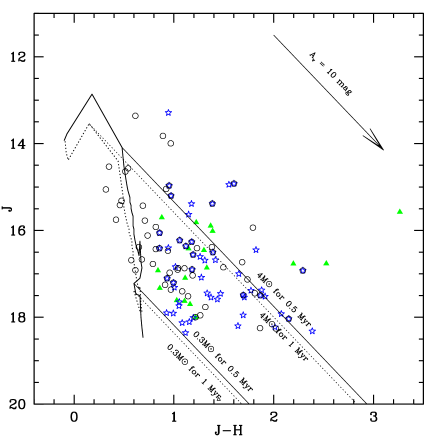
Figure 21: CM diagram for YSO candidates in Sh 2-100 SFR. The symbols are same as in Fig. 17. The PMS isochrone of 0.5 Myr (solid curve) and 1 Myr (dotted curve) from Siess et al. (2000) are drawn at a distance of 8.7 kpc and zero reddening. The reddening vectors corresponding to 0.3$M_{\odot}$ and 4$M_{\odot}$, are also shown in the figure.

Considering the presence of CH ii & UCH ii regions, astronomical masers and intense gas and dust, similar to the W3 Main region studied by Ojha et al. (2004b), we assumed PMS age of 0.5 Myr to 1 Myr for the YSOs to estimate their masses. To minimize the effect of NIR excess emission on mass estimation we preferred $J$-band luminosity rather than $H$ or $K$ band. Fig. 21 represents $(J-H)$ versus $J$ CM diagram for the YSOs. The solid and dotted curve lines in Fig. 21 denote the loci of 0.5 Myr and 1 Myr PMS isochrones by Siess et al. (2000). The solid and dotted slanting lines are the reddening vectors for 0.3 and 4 $M_{\odot}$ stars for the 0.5 Myr and 1 Myr isochrones, respectively. The different symbols represent the YSOs selected from NIR and IRAC CC diagram and are the same as in Fig. 17. The reddening vectors for the assumed age suggest that the majority of the YSOs have masses in the range of 0.3$M_{\odot}$ - 4$M_{\odot}$ indicating that stellar population in Sh 2-100 is mainly composed of low-mass YSOs. Although, the assumed age for the region is the subject of uncertainty and may not be accurate as compared to the ages estimated with the spectroscopic information of the sources in star clusters, the distibution of YSOs with wide colors (Fig. 21) probably indicates the combined effect of variable extinction, weak contribution of excess emission in $J$ and $H$ bands and/or sources in different evolutionary stages. Therefore, it would be very useful to get radial velocity information of the YSOs to confirm their association and ages with spectroscopic information.

7.5 A possible evolutionary status of the regions

The regions K3-50E and K3-50F contain massive B0-B0.5V MS stars. These early-type stars usually form in the dense core of a molecular cloud and can be seen in millimeter, mid-, far-infrared and/or as compact radio emissions. The presence of weak extended radio emission (Fig. 4) and lack of dust continuum emission at 25 $\mu$m and 60 $\mu$m (see Fig. 22) indicate that the associated regions are probably in an advanced stage of evolution. The presence of relatively intense radio emission at 1280 MHz and dust emission at 25 $\mu$m and 60 $\mu$m, respectively, indicate that K3-50D is younger or of age comparable with K3-50E & K3-50F. All the ionizing sources of these regions do not show infrared excess and their detection in the optical band suggests their evolved nature. The optical V/V-I diagram suggests that the age of the ionizing sources is of the order of 1 - 2 Myr. However, non-detection of ionzing source(s) in optical, relatively intense $K_{\rm s}$ -band emission as well as radio emission as compared to K3-50D suggest that K3-50B should be younger than K3-50D. The regions K3-50A and K3-50C (consisting of two sources C1 and C2) are possibly younger than K3-50B, due to their association with intense ¹²CO(1-0) emission, compact radio sizes and the ionzing sources possess infrared excess (e.g., C2 and A). The detection of OH masers (Baudry & Desmurs 2002) and ionized outflows (DePree et al. 1994; Balser et al. 2001) in both the cores indicate that they are not dynamically evolved objects and suggest that the star formation activity around K3-50C and K3-50A should not be more than $\sim$ few $\times$ 10⁵ yr. The component C1 is hidden behind a visual extinction $\geq$ 190 mag, therefore invisible in wavelength shorter than 20 $\mu$m, whereas the ionizing source of K3-50A is detected in NIR and embedded in molecular cloud having visual extinction $\sim$ 17.5 mag. K3-50C1 has lower dust temperature than K3-50A, possibly indicating that K3-50C1 is more deeply embedded in the molecular cloud as compared to K3-50A (Hunter et al. 1997). The above discussion reveals that K3-50C1 is most likely the youngest source of the region.

7.6 Star formation scenario in W58

W58 is a molecular cloud complex of an angular extent of about 60 arcmin. The ¹²CO distribution mainly reveals three distinct components (see Fig.3 of Israel 1980) and the associated SFRs to these components are K3-50, Sh 2-99 (S99) and W58G. Fig. 23 shows 8 $\mu$m emission from MSX A-band along with the distribution of H i emission around the SFR complex (thick solid line) taken from Fig. 6 of Israel (1980). The positions of different sources found towards the direction of W58 cloud complex are shown as crosses. The most intense northern CO component associated with K3-50 SFR peaks close to K3-50C, where most of the star formation activity is currently going on. The western CO component is associated with an optically visible region (Sh 2-99/G70.15+1.73) situated at a distance of $\sim$ 11^′ from K3-50A towards the south-western direction. The weaker southern CO component is associated with an region (W58G/G69.92+1.52) which is $\sim$ 23^′ away from K3-50A. In the case of region (W58G), a radial velocity of -65 km s^-1 has been measured, which differs significantly from the radial velocity - 22 to -25 km s^-1 found in the direction of W58. This indicates that W58G most likely is not related to W58 cloud complex (Israel 1980 and references therein), whereas the radial velocity of -22.9 km s^-1 for Sh 2-99 (Blair et al. 1975) suggests its association with W58.

With the help of H i emission observed by Read (1981) with a resolution of 2^′.5 $\times$ 4^′.6, Israel (1980) pointed out an H i /expanding shell of diameter $\sim$ 75 pc and suggested that the current star formation activity in Sh 2-99 and K3-50 region might have been induced by the interaction of this shell produced by stellar winds from the older generation stars of W58 cloud complex. To recognize such a shell, a potential way is to use the PAH emissions at 8 $\mu$m arising from the photodissociation region, which occurs at the interface between the molecular and neutral gas and thought to be excited by sub-Lyman UV photons from the massive star(s). Consequently, it can be used as a tracer of the neutral shell observed in the H i 21-cm line emission at the edge of expanding region (Deharveng et al. 2005). Fig. 23 shows the 8 $\mu$m PAH emission surrounding the bubble noticed by Israel (1980) and roughly coincides with the H i emission in terms of discrete patches. The absence of 8 $\mu$m emission in the interior of the H i shell can be interpreted as the destruction of PAH molecules by intense UV radiation from the associated massive star(s). The shape and large dimension of H i shell suggest that the stars producing stellar wind should be located inside the shell. A search of Simbad database results in a WR star (WR 131) of WN7h (hydrogen rich) subtype (Figer et al. 1997), whose position is marked in Fig. 23. The hydrogen rich WN7 stars are descendants of massive stars with initial masses above 50-60 $M_{\odot}$ (e.g., Crowther et al. 1995). Indeed, progenitors of such stars are believed to be core-hydrogen burning Of stars with strong stellar winds (Crowther et al. 1995). The presence of WR 131 in the H i shell and its approximate distance of $\sim$ 9.1 kpc (Georgelin et al. 1988) comparable with the distance estimates of W58 complex ($\sim$ 7.9 to 9.3 kpc), favors a probable association between the WR 131 and W58 complex. The catalog of Reed (1998) yields a few B-type stars which are projected inside the bubble, but their distances are not known so as to confirm their association. If indeed these sources are associated then the presence of H i shell can be due to the combined energy input from these sources.

WR 131 is not located at the center of the H i shell but at an off-center position, which could be due to the combination of an inhomogeneous medium, proper motion of the star, anisotropic winds and projection effect along the line of sight. If we assume WR 131 is the source to produce H i shell due to its strong stellar winds and since WR phase is short lived ($\sim$ 10⁵ yr) and the presence of WR star limits the maximal age $\sim$ 4.5 - 5 Myr of a cluster (Meynet & Maeder 2005), an upper limit of age $\sim$ 4 - 4.5 Myr can be assigned to WR 131, considering the estimated dynamical age ($\sim$ $10^{7}$ yr) of the bubble by Israel (1980). If the age of WR 131 is $\sim$ 4 - 4.5 Myr then one would expect the ages of the second generation stars, (if any), at the periphery of the bubble, should be less than that of a WR star. The presence of star formation activity, which might have started $\leq$ 2 Myr ago is evident at the north-eastern edge of the shell, with the existence of Class I sources, astronomical masers, UCH ii and CH ii regions containing young OB stars of ages 1-2 Myr. The presence of seven regions at different spatial locations and possibly at different evolutionary stages suggests star formation activity has proceeded at multiple sites in the cloud. The presence of WR 131 star of age $\sim$ 4 - 4.5 Myr and young massive stars still in accretion phase (e.g., C1 and A), associated with the same complex, indicates distribution of stars of different ages in the region. Israel (1980) suggested that at present the shell is colliding with a larger H i cloud to the northeast of W58 (i.e., east of K3-50C). In this conjuncture, one would expect Sh 2-99 and K3-50D to be relatively evolved regions and K3-50C to be the least evolved source as we move from southwest to northeast. On a large scale, it seems to be consistent with the scenario of sequential star formation because the probable age of K3-50D is $\sim$ 1 - 2 Myr, whereas the expected age of K3-50C1 is of $\sim$ few $\times$ 10⁵ yr. This is further supported by the presence of more intense molecular material observed towards K3-50C than Sh 2-99 (Israel 1980), along with the average extinction gradient of 4.2 to 97 mag from K3-50D to K3-50C1. However, it is not known whether the different condensations of Sh 2-100 region were in different stages of evolution before the passage of ionization front generated by the stellar winds of WR 131. It is also difficult to anticipate the projection/ orientation effect on the location of the WR star with respect to the Sh 2-100 region. The initial mass of the cloud associated with the individual region is also an important parameter as it governs evolution of the cloud in presence of external radiation pressure. Numerical models predict that if the pressure due to external ionized gas is too small to compress a massive molecular gas, the radiation field will not have any dynamic effect on the cloud (Bertoldi & McKee 1990; Lefloch & Lazareff 1994). At present the sequential star formation around Sh 2-100 region due to the interaction of H i bubble is suggestive. A more complete picture can be revealed with the help of high resolution, high sensitivity H i and CO observations covering the entire W58 complex. A positional and chronological study of the YSOs associated with the complex (e.g., Lee et al. 2005; Ogura 2006) can support the validity of sequential star formation. Since the region studied here is deeply embedded and shows a large variation in extinction, we would like to determine the intrinsic properties of the low mass PMS stars identified from the NIR and IRAC CC diagrams with follow up deep optical/NIR spectroscopic observations in order to determine their relative ages by constructing intrinsic Hertzsprung-Russell diagrams. These observations will allow us to have a better understanding of star formation history across the entire region and a much clearer picture of the triggered star formation across the W58 complex.

8 Conclusions

In this paper we have presented a multi-wavelength study of the stellar contents and physical environment of star-forming region (K3-50) in the proximity of diffuse region Sh 2-100. K3-50 consists of seven regions (A, B, C1, C2, D, E and F) of different classes and are thought to be a part of W58 molecular cloud complex located at a distance of $\sim$ 8.7 kpc. Our main conclusions are as follows:

1. We have identified the ionizing star of the optical visible nebula K3-50D. Optical spectroscopy suggests that an O4V star is responsible for the ionization. We have estimated a distance of $\sim$ 8.6 kpc for the K3-50D region. The approximate distances for the K3-50E and K3-50F regions have been estimated from the NIR photometry and radio continuum flux densities following the methodology by Comerón & Torra (2001). The distance estimation suggests that both the regions are likely the part of the W58 complex.

2. We identified the probable exciting sources for six regions using the $J$ vs. $J-H$ CM diagram. The photometric spectral types of the ionizing sources agree well within a subclass with that derived from radio observations based on the number of Lyc photons.

3. We derived physical parameters for all the five regions using 1280 MHz radio continuum observation. The regions cover a wide range in size ($\sim$ 0.2 to 1.6 pc), optical depth ($\sim$ 0.18 to 1.92), rms electron density ($\sim$ 740 to 6390 cm^-3) and rate of Lyc photons ($\sim$ 5.5 $\times$ 10⁴⁷ s^-1 to $\sim$ 1.1 $\times$ 10⁴⁹ s^-1). These physical parameters reflect different evolutionary stages of regions.

4. We estimated the total mass of the cloud associated with one of the regions (K3-50A) which was found to be $\sim$ 7800 $M_{\odot}$. At the center of the cloud core, we detected a possible massive YSO with $M_{\star}$ $\sim$ 42 $\pm$ 4.4 $M_{\odot}$, accreting with an effective envelope accretion rate of Log($\dot{M}_{env}$) $\sim$ -3.8$\pm$ 0.2 $M_{\odot}$ yr^-1.

5. Combining IRAC photometry with ground-based NIR observations within an area of $\sim$ 8^′ $\times$ 8^′, we found a total of 150 objects with circumstellar disks (i.e., YSOs), suggesting a site of active star formation. The distribution of these YSOs (Class II, Class I and $H-K$ $>$ 1.8 sources) in Sh 2-100 SFR correlates well with the association of gas and dust within the region.

6. The distribution of YSOs at the periphery of H i shell on a large scale supports the speculation by Israel (1980) that the star formation activity around K3-50 region might have been induced by an expanding spherical bubble which was created by strong stellar winds from older generation OB stars of the complex in the south-eastern direction.

The Sh 2-100 SFR region represents a broad sample of different stages of massive star formation all in the same cloud, from the cold, dense core at source C1 to the diffuse H II region at source F. The conclusions drawn in this paper on this cloud should be relevant and applicable to further deep study of the region with high resolution and high sensitivity instruments.

9 Acknowledgments

We thank the anonymous referee for a critical reading of the paper and several useful comments and suggestions, which greatly improved the scientific content of the paper. The authors would like to thank the staff of HCT operated by Indian Institute of Astrophysics, Bangalore, IRSF at South Africa in joint partnership between S.A.A.O and Nagoya University of Japan and GMRT managed by National Center for Radio Astrophysics of the Tata Institute of Fundamental Research (TIFR) for their assistance and support during observations. MRS would like to thank the TIFR for the kind hospitality during his visits to the institute, where a part of the work reported was carried out. MRS also thanks T. P. Prabhu and A. Tej for helpful discussions, as well as N. Chauhan and J. Jose for their helpful discussions on the Spitzer data reduction.

Appendix A: Selected interesting region

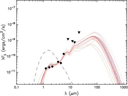
Figure 24: $Left$: $JHK$ color-composite image around IRAS-B region. $Right$: SED of the luminous source associated with IRAS-B. The filled circles represent NIR and Spitzer flux values, whereas the filled triangles denote upper limit of the MSX flux values. The solid lines show all models that fit the data reasonably with ${\chi}^{2}-{\chi_{best}}^{2}<3$ . The dashed line shows the SED of the stellar photosphere in the best-fitting model.

IRAS-B is situated at $\sim$ 3^′.3 northwest of K3-50A. An analysis of the IRAS fluxes reveals that this source has color characteristics (e.g., log (F25 )/log (F12 ) = 2.02 and log (F60 )/log (F12) = 5.06) consistent with being an UCH ii region (Wood & Churchwell 1989). A prominent $K_{\rm s}$-band nebulosity seen in the direction of IRAS-B is offset by $\sim$ 15^′′ in the western direction from the position of IRAS-B (see Fig. 24). Our NIR images reveal that the $K_{\rm s}$-band nebulosity contains few point sources and the position of the MSX point source (G070.3164+01.6493) falls on the $K_{\rm s}$-band nebulosity. The offset of IRAS-B may be due to the large IRAS beam. Therefore, the more accurate position of the IR source associated with IRAS-B can be inferred from the nearby MSX point source (G070.3164+01.6493), since the MSX survey has global absolute astrometric accuracy of 1^′′.9. The MSX CC plot (see Fig. 18) for the source suggests IRAS-B to be a massive YSO. Since there is no study available in the literature for IRAS-B, the distance to the source is unknown, which puts a limit to support in favor of a physical connection of this source with Sh 2-100, rather than a chance of alignment along the line of sight. However, if we assume a distance 8.7 kpc, our analysis leads to many useful conclusions. We acknowledge that this assumption is highly speculative, hence the results should be taken with caution. Analysis of NIR CM and CC diagrams suggest that the most luminous member associated with IRAS-B is a ZAMS star of spectral type $\sim$ O7-O8 with NIR excess. Since the source shows NIR excess, the spectral class assigned on the basis of CM diagram could have been estimated as an early type rather than its real spectral type, but this still disagrees with the ZAMS spectral type (earlier than O3) derived from IRAS point source fluxes using the equation of Casoli et al. (1986). This discrepancy could be due to large IRAS beam and/or presence of low mass stars, which can contribute significantly to the radiation emitted in the FIR. If we assume that an O8 star is present in the region, the absence of radio emission (up to $\sim$ 5 mJy) at 1280 MHz indicates that (i) either the ionizing star is heavily enshrouded by the dust so that all its ionizing radiation is absorbed or (ii) the region is suppressed by the accretion of matter (see, e.g., Yorke 1986) or (iii) the source must be a ZAMS star of spectral type later than B0. The spectral type B0 has been estimated from the Lyc photons derived using $\sim$ 5 mJy flux (3$\sigma$ flux of the map at 1280 MHz) and the calibration table of Panagia (1973), for an electron temperature of 10⁴ K. In order to get a qualitative estimation of the evolutionary stage of the source, we have fitted the models by Robitaille et al. (2006), which are already described in section 6.2.3. The SED is shown in Fig. 24. Though, the number of data points used for the SED fitting are quite less, nevertheless as stated by Robitaille et al (2007), some of the parameters can be constrained more narrowly than the others, depending upon the available fluxes. The parameters computed from the models as described in section 6.2.3, imply a source of mass $M_{\star}$ = 10.7 $\pm$ 1.8 $M_{\odot}$ and total luminosity Log$L_{\star}$ = 3.4 $\pm$ 0.2 $L_{\odot}$ lying behind 6.1 $\pm$ 0.2 mag of visual extinction. In the absence of sub-mm and mm data points, the resulting uncertainties in other parameters may be large, and therefore not quoted here. The mass of the object suggests a star of spectral type B2-B3V, but the lack of radio emission around the star at such a low visual extinction requires follow up high sensitivity, high frequency radio observations, along with $K_{\rm s}$-band spectroscopy to obtain the accurate nature of the massive star and its distance.

Table 1: Log of observational data.

Date (UT)	Filter	No of	Exposure (sec)	Telescope
		frames	per frame
2006 Oct 24	U	3	1000	ST
2006 Oct 25	U	3	300	ST
2006 Oct 24	B	3	900	ST
2006 Oct 25	B	3	300	ST
2006 Oct 24	V	3	600	ST
2006 Oct 25	V	3	100	ST
2007 Oct 29	Gr 7	1	900	HCT
2007 June 18	Gr 7	2	900	HCT
2008 July 21	J	120	10	IRSF
2008 July 21	H	120	10	IRSF
2008 July 21	Ks	120	10	IRSF
2007 June 18	H$\alpha$	1	300	HCT
2007 June 18	R	1	300	HCT
2007 June 18	[SII]	1	300	HCT
2004 Oct 10	Br$\gamma$	21	90	HCT
2004 Oct 10	Kcont	21	20	HCT

Table 2: Details of the GMRT radio continuum observations.

Rest freq. (MHz)	1280	610
Date of Obs.	25 Jan 2004	07 Apr 2004
Phase center	$\alpha_{2000}=20^{h}01^{m}45.50^{s}$	$\alpha_{2000}=20^{h}01^{m}45.50^{s}$
	$\delta_{2000}=33^{h}32^{m}43.02^{s}$	$\delta_{2000}=33^{h}32^{m}43.02^{s}$
Flux calibrator	3C48	3C286
Phase calibrator	2052+365	1924+334
On source int. time	1 (hr)	3 (hr)
Cont. Bandwidth	16 (MHz)	16 (MHz)
Synth. beam	3″.3 $\times$ 3″.0	5″.5 $\times$ 4″.8
rms noise	2.2 mJy/beam	0.9 mJy/beam

Table 3: Observed integrated flux and angular size for associated regions

Frequency			1280 MHz	1280 MHz
Source	Peak Position		Int. Flux	Angular Size
	$\alpha$(J2000)	$\delta$(J2000)	Jy
A	20:01:45.57	+33:32:42.86	0.387	7′′.1 $\times$ 4′′.6
B	20:01:48.01	+33:33:03.21	1.680	36′′.4 $\times$ 33′′.3
C1	20:01:53.87	+33:34:15.52	0.156	8′′.2 $\times$ 5′′.3
C2	20:01:55.08	+33:34:16.44	0.093	5′′.8 $\times$ 4′′.2
D	20:01:47.67	+33:31:50.61	1.880	42′′.9 $\times$ 37′′.8

Table 4: Derived parameters for the regions from radio observations

Source	$\tau_{c}$	rms $n_{e}$	EM	log NLyc	ZAMS${\dagger}$
		(103 cm-3)	(106 cm-6 pc)	(ph. s-1)	Spectral type
A	1.92	6.39	9.84	48.36	O8
B	0.22	0.88	1.14	49.00	O6
C1	1.38	5.04	7.07	48.34	O8
C2	0.84	4.89	4.28	47.74	O9.5
D	0.18	0.74	0.95	49.04	O6.5

Table 5: Spectral types of the ionizing sources of the regions

	Spectral Type
Source	NIR estimation ${\dagger}$	Radio estimation (Ref.)
A	$>$ O5	O5.5 (1)
B	O5	O5.5 (1)
C1	—	O9 (1)
C2	B0-O9.5	O9.5 (1)
D	O5	O6 (1)
E	B0.5	O8 (2)
F	B0	O9.5 (2)

Table 6: Observed and dereddened line intensities derived from the optical spectrum of K3-50A nebula

$\lambda$ (Å)	Lines	Obs. Flux ${\dagger}$	Dered. Flux ${\ddagger}$
3726, 9	[O ii]	0.299	3.121
4340	H$\gamma$	0.189	0.591
4861	H$\beta$	1.000	1.000
4959	[O iii]	0.502	0.416
5007	[O iii]	1.814	1.378
5755	[N ii]	0.059	0.016
5876	He i	0.412	0.094
6548	[N ii]	1.796	0.208
6563	H$\alpha$	24.79	2.839
6583	[N ii]	6.74	0.758
6678	He i	0.281	0.029
6717	[S ii]	0.502	0.050
6731	[S ii]	0.932	0.091
7065	He i	0.457	0.032
7136	[Ar iii]	0.986	0.065
7319, 20	[O ii]	0.350	0.019
7330, 31	[O ii]	0.733	0.040

Figure 1: POSS II $R$-band image of the region around Sh 2-100. The names (A, B, C1, C2, D, E and F) represent the different associated regions namely K3-50A, K3-50B, K3-50C1, K3-50C2, K3-50D, K3-50E and K3-50F, respectively, following the nomenclature by Israel (1976). The RA and DEC coordinates are in J2000.0 epoch.

Figure 2: Comparison of IRSF/SIRIUS $JHK_{\rm s}$ photometry with the 2MASS data for the common sources. The difference $\Delta$ (IRSF - 2MASS) in mag is plotted as a function of $J$ mag.

Figure 3: $JHK_{\rm s}$ color-composite image of the Sh 2-100 star-forming region ($J$, blue; $H$, green; and $K_{\rm s}$ , red). Locations of the different regions are also marked. The rectangular box shown by white lines to the left represents the region selected as relative control field (see §5.1). The enhanced green color seen below the region D is the artifact of the $H$-band due to a bright star. North is up and east is to the left.

Figure 4: IRSF $K_{\rm s}$-band image in logarithmic scale overlaid by the GMRT radio continuum contours at 610 MHz. The contour levels are at 0.88 $\times$ (3, 5, 8, 12, 17, 22, 28, 35, 43, 51, 70, 81, 93, 102) mJy/beam, where $\sim$ 0.88 mJy/beam is the rms noise in the map at the resolution of $\sim$ $5\arcsec.5\times 4\arcsec.8$. Individual regions are also marked in the figure. The labelled axes are in J2000 coordinates.

Figure 8: (a) CC diagram for the sources within 0.5 pc radius of the regions. The giant, dwarf, CTT loci and the reddening vectors are plotted in a similar manner as in Fig. 6$c$. (b) $J-H$ vs. $J$ CM diagram for the same sources with their $Q$ values. The nearly vertical solid lines represent the ZAMS loci at a distance of 8.7 kpc reddened by $A_{\rm V}$ = 0, 10 and 20 mag. The slanting lines show the reddening vectors corresponding to ZAMS spectral type.

Figure 9: Spatial distribution of the sources found within 0.5 pc radius of each region superposed on the $K_{\rm s}$-band image. The sources are labeled with numbers corresponding to the regions. North is up and east is to the left.

Figure 11: (a) The blue part of the spectrum of the most luminous star (V $\sim$ 13.31 mag) of K3-50D, displaying characteristics similar to $\sim$ O4 MS member. (b) The $(U-B)/(B-V)$ CC diagram for the stars lying within 50^′′ of K3-50D region. The continuous curve represents intrinsic ZAMS by Schmidt-Kaler (1982), shifted along the reddening vector of 0.72 slope for $E(B-V)_{min}$ = 1.36 mag.

Figure 14: SED for the luminous source (A1) at the center of K3-50A region. The filled circles represent flux values while the triangles denote upper limits of the flux values. The solid lines show all the models that fit the data reasonably with ${\chi}^{2}-{\chi_{best}}^{2}<3$. The dashed line shows the SED of the stellar photosphere in the best-fitting model.

Figure 15: The blue part of the optical spectrum of the star B3 of K3-50B region.

Figure 17: The spatial distributions of Class II (asterisks), Class I (filled triangles), sources detected only in $H$ and $K_{s}$ bands with $H-K$ $\geq$ 1.8 (filled circles), YSOs detected from $H-K/K-[4.5]$ CC diagram (open circles) and MSX point sources (crosses), overlaid on $K_{\rm s}$-band image (for color plot see online electronic version). The thin contours represent ¹²CO emission from Israel (1980) at a resolution of 2^′.3 integrated over a velocity range of 13 km s^-1. The thin white contours represent 8 $\mu$m emission from Spitzer. The contours start at 54 MJy sr^-1 ($\sim$ 3$\sigma$, where $\sigma$ is the rms noise of the map) and the innermost contour corresponds to a value of 450 MJy sr^-1. North is up and east is to the left.

Figure 18: CC plot for the MSX point sources around Sh 2-100 region. The limits derived by Lumsden et al. (2002) for massive YSOs and regions (dashed lines) are mentioned by their areas. The numbers represent the MSX point sources associated with different regions and are mentioned in the upper left corner of the figure.

Figure 19: SEDS of bright NIR sources within individual regions having IRAC counterparts.

Figure 20: The intrinsic $V/B-V$ CM diagram for the ionizing stars of K3-50D, K3-50E and K3-50F regions. The solid line shows the theoretical isochrones taken from Girardi et al. (2002) for 1 Myr at a distance of 8.7 kpc.

Figure 22: 2MASS $K_{\rm s}$-band image overlaid with the warm dust contours at 25 $\mu$m (black in color) and cold dust contours at 60 $\mu$m (white in color) taken from HIRES processed images of IRAS. The 25 $\mu$m contour levels are at 1.5, 2, 3, 4, 5, 10, 20, 40, 60, 80, 90 % of the peak value 43208 MJy sr^-1 and the 60 $\mu$m contour levels are at 1.5, 2, 3, 5, 7, 10, 15, 20, 25, 40, 60, 80, 90% of the peak value 44942 MJy sr^-1. Locations of the individual regions are also marked. The labelled axes are in J2000 coordinates.

Figure 23: MSX A-band image marked with area of H i emission (thick solid line) taken from Israel (1980). The crosses represent the positions of different sources in the W58 cloud complex (see the text). North is up and east is to the left.

References

- (1) Allen, L. E., et al. 2004, ApJS, 154, 363
- (2) Alvarez, C., Feldt, M., Henning, Th., Puga, E., Brandner, W., & Stecklum, B. 2004, ApJS,155, 123
- (3) Araya, E., Hofner, P., Churchwell, E., & Kurtz, S. 2002, ApJS, 138, 63
- (4) Aumann, H. H., Fowler, J. W., & Melnyk, M. 1990, AJ, 99, 1674
- (5) Balser, D. S., Goss, W. M., & De Pree, C. G. 2001, AJ, 121, 371
- (6) Baudry, A., & Desmurs, J. F. 2002, A&A, 394, 107
- (7) Bernasconi, P. A., & Maeder, A. 1996, A&A, 307, 829
- (8) Bertoldi, F., & McKee, C. F. 1990, ApJ, 354, 529
- (9) Bessell, M. S., & Brett, J. M. 1988, PASP, 100, 1134
- (10) Beuther, H., Schilke, P., Sridharan, T. K., Menten, K. M., Walmsley, C. M., & Wyrowski, F. 2002, A&A, 383, 892
- (11) Beuther, H., Churchwell, E. B., McKee, C. F., & Tan, J. C. 2007, in Protostars and Planets V, eds. B. Reipurth, D. Jewitt, & K. Keil (Tucson, AZ: Univ. Arizona Press), 165
- (12) Bik, A., Kaper, L., Waters, L. B. F. M., 2006, A&A, 455, 561
- (13) Blair, G. N., Peters, W. L., & Vanden Bout, P. A. 1975, ApJ, 200, L161
- (14) Bronfman, L., Nyman L.-A., May, T. 1996, A&AS, 115, 81
- (15) Cardelli, J. A., Clayton, G. C., & Mathis, J. S. 1989, ApJ, 345, 245
- (16) Casoli, F., Combes, F., Dupraz, C., Gerin, M., & Boulanger, F. 1986, A&A, 169, 281
- (17) Cohen, J. G., Persson, S. E., Elias, J. H., & Frogel, J. A. 1981, ApJ, 249, 481
- (18) Camerón, F., & Torra, J. 2001, A&A, 375, 539
- (19) Comerón, F., & Pasquali, A. 2005, A&A, 430, 541
- (20) Conti, P. S. 1988, in O Stars and Wolf-Rayet Stars, eds. P. S. Conti et al. (NASA SP-497; Washington), 119
- (21) Cox, A. N. 2000, Allen’s Astrophysical Quantities, Fourth edition (New York: AIP Press; Springer), ed. Arthur N. Cox
- (22) Crowther, P. A., Smith, L. J., Hillier, D. J., & Schmutz, W. 1995, A&A, 293, 427
- (23) Cutri, R. M., et al. 2003, 2MASS All-Sky Catalog of Point Sources (Pasadena: NASA / IPAC), http://irsa.ipac.caltech.edu /applications/Gator
- (24) Dobashi, K., Yonekura, Y., Matsumoto, T., Momose, M., Sato, F., Bernard, J.-P., & Ogawa, H. 2001, PASJ, 53, 85
- (25) DePree, C. G., Goss, W. M., Palmer, P., & Rubin, R. H. 1994, ApJ, 428, 670
- (26) Deharveng, L., Zavagno, A., & Caplan, J. 2005, A&A, 433, 565
- (27) Egan, M. P., et al. 2003, MSX6C Infrared Point Source Catalog (AFRL-VS- TR-2003-1589; Bedford: AFCRL)
- (28) Fazio, G. G., et al. 2004a, ApJS, 154, 10
- (29) Fazio, G. G. et al. 2004b, ApJS, 154, 39
- (30) Figer, D. F., McLean, I. S., & Najarro, F. 1997, ApJ, 486, 420
- (31) Flaherty, K. M., Pipher, J. L., Megeath, S. T., Winston, E. M., Gutermuth, R. A., Muzerolle, J., Allen, L. E., & Fazio, G. G. 2007, ApJ, 663, 1069
- (32) Garay, G., Rodriguez, L. F., Moran, J. M., & Churchwell, E. 1993, ApJ, 418, 368
- (33) Garay, G., & Lizano, S. 1999, PASP, 111, 1049
- (34) Georgelin, Y. M. 1975, These d’Etat, Univ. de Provence (Univ. d’Aix Marseille I)
- (35) Georgelin, Y. M., Boulesteix, J., Georgelin, Y. P., Le Coarer E., Marcelin M., & Monnet, G. 1988, A&A, 190, 61
- (36) Girardi, L., Bertelli, G., Bressan, A., Chiosi, C., Groenewegen, M. A. T., Marigo, P., Salasnich, B., & Wiess, A. 2002, A&A, 391, 195
- (37) Grave, J. M. C., & Kumar, M. S. N., 2009, A&A, 498, 147
- (38) Gutermuth, R. A. et al. 2008, ApJ, 674, 336
- (39) Harris, S. 1975, MNRAS, 170, 139
- (40) Haslam, C. G. T., Salter, C. J., Stoffel, H., & Wilson, W. E. 1982, A&AS, 47, 1
- (41) Hildebrand, R. H. 1983, QJRAS, 24, 267
- (42) Hillenbrand, L. A., Strom, S. E., Vrba, F. J., & Keene, J. 1992, ApJ, 397, 613
- (43) Hillenbrand, L. A., Massey, P., Strom, S. E., & Merrill, K. M. 1993, AJ, 106, 1906
- (44) Horne, K. 1986, PASP, 98, 609
- (45) Hunter, T. R. 1997, PhD thesis, California Institute of Technology
- (46) Israel, F. P. 1976, A&A, 48, 193
- (47) Israel, F. P. 1980, ApJ, 236, 465
- (48) Johnson, H. L., & Morgan, W. W. 1953, ApJ, 117, 313
- (49) Kennicutt, R. C. Jr., Bresolin, F., French, H., & Martin, P. 2000, ApJ, 537, 589
- (50) Kerton, C. R., Martin, P. G., Johnstone, D., Ballantyne, D. R., 2001, ApJ, 552, 601
- (51) Kurtz, S., Churchwell, E., & Wood, D. O. S. 1994, ApJS, 91, 659
- (52) Kurtz, S., Cesaroni, R., Churchwell, E., Hofner, P., & Walmsley, C. M. 2000, in Protostars and Planets IV, eds. V. Mannings, A. P. Boss, & S. S. Russell (Tucson, AZ: Univ. Arizona Press), 299
- (53) Kurtz, S., & Hofner, P. 2005, AJ, 130, 711
- (54) Landolt, A. U. 1992, AJ, 104, 340
- (55) Lee, H.-T., Chen, W. P., Zhang, Z.-W., & Hu, J.-Y. 2005, ApJ, 624, 808
- (56) Lefloch, B., & Lazareff, B. 1994, A&A, 289, 559
- (57) Lumsden, S. L., Hoare, M. G., Oudmaijer, R. D., & Richards, D. 2002, MNRAS, 336, L621
- (58) Massey, P., Strobel, K., Barnes, J. V., & Anderson, E. 1988, ApJ, 328, 315
- (59) Megeath, S. T., et al. 2004, ApJS, 154, 367
- (60) Martins, F., Schaerer, D., & Hillier, D. J. 2005, A&A, 436, 1049
- (61) Meyer, M. R., Calvet, N., & Hillenbrand, L. A. 1997, AJ, 114, 288
- (62) Meynet, G., Maeder, A., Schaller, G., Schaerer, D., & Charbonnel, C. 1994, A&AS, 103, 97
- (63) Meynet, G., & Maeder, A. 2005, A&A, 429, 581
- (64) Mezger, P. G., & Henderson, A. P. 1967, ApJ, 147, 471
- (65) Nagashima, C., et al. 1999, in Proc. Star Formation 1999, ed. T. Nakamoto (Nagano: Nobeyama Radio Obs.), 387
- (66) Nagayama, T., et al. 2003, Proc. SPIE, 4841, 459
- (67) Neugebauer, G., & Garmire, G. 1970, ApJ, 161, L91
- (68) Ojha, D. K., Ghosh, S. K., Kulkarni, V. K., Testi, L., Verma, R. P., & Vig, S. 2004a, A&A, 415, 1039
- (69) Ojha, D. K., et al. 2004b, ApJ, 608, 797
- (70) ——. 2004c, ApJ, 616, 1042
- (71) Okamoto, Y. K., Kataza, H., Yamashita, T., et al. 2003, ApJ, 584, 368
- (72) Osterbrock D. E., 1989, Astrophysics of Gaseous Nebulae and Active Galactic Nuclei. University Science Books, Mill Valley, CA
- (73) Ogura, K. 2006, Bull. Astron. Soc. India, 34, 111
- (74) Palla, F., & Stahler, S. W. 1990, ApJ, 360, L47
- (75) Panagia, N. 1973, AJ, 78, 929
- (76) Panagia, N. & Walmsley, C. M. 1978, A&A, 70, 411
- (77) Pandey, A.K., Sharma, S., Ogura, K., Ojha, D.K., Chen, W.P., Bhatt, B.C., & Ghosh, S.K. 2008, MNRAS, 383, 1241
- (78) Patten, B. M. et al. 2006, ApJ, 651, 502
- (79) Persi, P., Tapia, M., & Roth, M. 2000, A&A, 357, 1020
- (80) Persson, S. E., & Frogel, J. A. 1974, ApJ, 188, 523
- (81) Phillips, J. P., & Mampaso, A. 1991, A&AS, 88, 189
- (82) Price, S. D., Egan, M. P., Carey, S. J., Mizuno, D. R., & Kuchar, T. A. 2001, AJ 121, 2819
- (83) Read, P. R. 1981, MNRAS, 195, 371
- (84) Reed, B. C. 1998, ApJS, 115, 271
- (85) Robitaille, T. P., Whitney, B. A., Indebetouw, R., Wo od, K., & Denzmore, P. 2006, ApJS, 167, 256
- (86) Robitaille, T. P., Whitney, B. A., Indebetouw, R., & Wood, K. 2007, ApJS, 169, 328
- (87) Roelfsema, P. R., Goss, W. M., & Geballe, T. R. 1988, A&A, 207, 132
- (88) Samal, M. R., Pandey, A. K., Ojha, D. K., Ghosh, S. K., Kulkarni, V. K., & Bhatt, B. C. 2007, ApJ, 671, 555
- (89) Schmidt-Kaler, Th. 1982, Landolt-Bornstein, Vol. 2b, ed. K. Schaifers, H. H. Voigt & H. Landolt (Berlin: Springer), 19
- (90) Shepherd, D. S., & Churchwell, E. 1996, ApJ, 472, 225
- (91) Sharpless, S. 1959, ApJS, 4, 257
- (92) Shaw, R. A., & Dufour, R. J. 1994, in ASP Conf. Ser. 61, Astronomical Data Analysis Software and Systems III, eds. D. R. Crabtree, R. J. Hanisch, & J. Barnes (San Francisco: ASP), 327
- (93) Stern, D. et al. 2005, ApJ, 631, 163
- (94) Siess, L., Dufour, E., & Forestini, M., 2000, A&A, 358,593
- (95) Stetson, P. B. 1987, PASP, 99, 191
- (96) Swarup, G., Ananthakrishnan, S., Kapahi, V. K., Rao, A. P., Subrahmanya, C. R., & Kulkarni, V. K., 1991, Current Science, 60, 95
- (97) Tej, A., Ojha, D. K., Ghosh, S. K., Kulkarni, V. K., Verma, R. P., Vig, S., & Prabhu, T. P. 2006, A&A, 452, 203
- (98) Thompson, M. A., Hatchell J., Walsh, A. J., MacDonald, G. H., & Millar, T. J. 2006, A&A, 453, 1003
- (99) Thronson, H. A. Jr., & Harper, D. A. 1979, ApJ, 230, 133
- (100) Vacca, W. D., Garmany, C. D., & Shull, J. M. 1996, ApJ, 460, 914
- (101) Vogel, S. N., & Welch, W. J. 1983, ApJ, 269, 568
- (102) Walborn, N. R., & Fitzpatrick, E. L. 1990, PASP, 102, 379
- (103) Whitney, B.A., Wood, K., Bjorkman, J. E., & Wolff, M. J. 2003a, ApJ, 591, 1049
- (104) Whitney, B. A., Wood, K., Bjorkman, J. E., & Cohen, M. 2003b, ApJ, 598, 1079
- (105) Wood, D. O. S., & Churchwell, E. 1989, ApJS, 69, 831
- (106) Wynn-Williams, C. G., Matthews, K., Werner M. W., Becklin, E. E., & Neugebauer, G. 1977, MNRAS, 179, 255
- (107) Yorke, H. W. 1986, ARA&A, 24, 49