Classical approach in quantum physics

Abstract

The application of a classical approach to various quantum problems - the secular perturbation approach to quantization of a hydrogen atom in external fields and a helium atom, the adiabatic switching method for calculation of a semiclassical spectrum of hydrogen atom in crossed electric and magnetic fields, a spontaneous decay of excited states of a hydrogen atom, Gutzwiller’s approach to Stark problem, long-lived excited states of a helium atom recently discovered with the help of Poincar$\acute{\mathrm{e}}$ section, inelastic transitions in slow and fast electron-atom and ion-atom collisions - is reviewed. Further, a classical representation in quantum theory is discussed. In this representation the quantum states are treating as an ensemble of classical states. This approach opens the way to an accurate description of the initial and final states in classical trajectory Monte Carlo (CTMC) method and a purely classical explanation of tunneling phenomenon. The general aspects of the structure of the semiclassical series such as renormgroup symmetry, criterion of accuracy and so on are reviewed as well. In conclusion, the relation between quantum theory, classical physics and measurement is discussed.

1 Introduction

Classical physics is the foundation-stone in understanding of a microcosm, since all experimental devices are designed on classical principles. A classical approach can be used as an approximation in quantum physics also providing, sometimes, a more adequate description of dynamics than standard quantum approximations. The presented treatment involves all necessary quantum properties and the word ’classical’ in the title of this paper is used just to emphasize that this review (beside Sec.5) is based on the analysis of classical trajectories - not on the Schrödinger equation in semiclassical approximation. Besides, the classical approach to the real physical problems, for which an accurate asymptotic description can be developed, is presented, and original papers are cited only. The abstract problems, such as billiard models, Feigenbaum Universality and etc., are not discussed here since they are rather part of mathematics than physics.

The classical approach plays a fundamental role in quantum mechanics. Our understanding of any result in quantum theory relies upon classical language. For instance, since the degree of freedom ’spin’ has no analogue in classical mechanics, we have no idea how it looks like. The classical approach has also an advantage over different quantum approximations because of a more adequate description of dynamics of the system.

The semiclassical quantization conditions are formulated in the configuration space:

$$\int^{s_{2}}_{s_{1}}{p}(s)ds=\pi(k+\alpha_{1}+\alpha_{2})\hbar\ ,\ \ \ k=0,1,2,...$$ (1.1)

where $s_{1}$ and $s_{2}$ are caustics of a classical motion along the variable $s$ of the coordinate system where the Schödinger equation can be separated, and $\alpha_{1}$ and $\alpha_{2}$ are purely quantum phase shifts (so-called Morse indices) originating from the caustics; in the case of turning point $\alpha=\frac{1}{4}$, in the case of Coulomb singularity $\alpha=-\frac{1}{4}$ and in the case of the rotational motion $\alpha=0$. In contrast to classical mechanics, the quantization condition (1.1) is not invariant with respect to canonical transformations [1]. For instance, in action-angle variables $\{I,\varphi\}$ obtained from the set $\{p_{q},q\}$ by a canonical transformation, the motion is always a uniform rotation ($I=const,\varphi=\omega t$) and we lose the information about the type of caustics (turning points) which play a key role in quantization conditions.

For the isotropic potential $V(r)$ the problem is separable in the spherical coordinate $\{r,\vartheta,\varphi\}$ and Hamiltonian takes the form

$$H=\frac{1}{2m_{e}}\Bigl{[}{p_{r}}^{2}+\frac{1}{r^{2}}\Bigl{(}{p_{\vartheta}}^{2}+\frac{{p_{\varphi}}^{2}}{\sin^{2}\vartheta}\Bigr{)}\Bigr{]}+V(r),$$ (1.2)

where $m_{e}$ is the mass of the particle, $p_{r}=m_{e}\dot{r}$, $p_{\vartheta}=m_{e}r^{2}\dot{\vartheta}$ and $p_{\varphi}=m_{e}r^{2}\sin^{2}\vartheta\dot{\varphi}$ are canonically conjugate momenta to coordinates $r,\ \vartheta$ and $\varphi$, respectively. Since particle rotates uniformly along $\varphi$, $p_{\varphi}$ is conserved, caustics are absent and quantization condition (1.1) gives:

$$p_{\varphi}=m\hbar\ ,\ \ \ \ m=0,\pm 1,\pm 2,...,$$ (1.3)

The motion along $\vartheta$ variable is oscillation between two turning points $\vartheta_{1}=\arcsin(m\hbar/L)$ and $\vartheta_{2}=\pi-\arcsin(m\hbar/L)$, where $L$ is an angular momentum which is obtained from the quantization condition

$$\int_{\vartheta_{1}}^{\vartheta_{2}}\sqrt{L^{2}-\frac{m^{2}\hbar^{2}}{\sin^{2}\vartheta}}d\vartheta=(l+1/2)\hbar\ ,\ \ l=|m|,|m|+1,...,$$ (1.4)

as $L=(l+1/2)\hbar$ beside one exception - $l=0$. In this case we should accept value $L=0$ which follows from quantum treatment. At last, the energy level $E_{n_{r}l}$ for $l\neq 0$ is determined from the radial quantization condition

$$\int_{r_{1}}^{r_{2}}\sqrt{2m_{e}\Bigl{[}E_{n_{r}l}-V(r)-\frac{L^{2}}{2m_{e}r^{2}}\Bigr{]}}dr=(n_{r}+1/2)\hbar\ ,\ \ n_{r}=0,1,2,....$$ (1.5)

The quantization condition (1.5) gives correct value of energies even for the low lying levels since in this case the actual potential can be approximated by a parabolic well for which semiclassical and quantum spectra coincide. In the case $l=0$ ($L=0$), the quantization condition (1.5) depends on the type of inner caustic $r_{1}$. For Coulomb attraction $\alpha_{1}=-1/4$ and it compensates the contribution from the outer turning point $\alpha_{2}=1/4$ providing correct energy value.

Another general aspect is the use of the asymptotic techniques. The semiclassical approximation or the perturbation theory is the asymptotic series over a small parameter $\lambda$: $\sum_{n}a_{n}\lambda^{n}$. In the first case $\lambda=\hbar^{2}$, and in the second $\lambda$ is the amplitude of perturbation. Originally the asymptotic term $\{a_{n}\lambda^{n}\}$ is the estimation of the accuracy in the $(n-1)$-st order. At the beginning the terms $a_{n}\lambda^{n}$ decrease with increasing $n$ up to some index $n=n_{min}(\lambda)$. After that the terms start to increase and we lose the accuracy. The term $a_{n}\lambda^{n}$ can be considered as a correction only if the next term is smaller. Since the larger $\lambda$ the smaller $n_{min}(\lambda)$ is, in application, the leading term gives the correct result in the widest interval of $\lambda$ and we do not need any corrections which gradually lose the meaning of correction with increasing $\lambda$.

Atomic units ($m_{e}=e=\hbar=1$) are used throughout the review, unless otherwise explicitly indicated.

2 Energy spectrum and resonances

2.1 Secular perturbation theory

In the secular perturbation theory the Hamiltonian has the form $H({\bi p},{\bi r})=H_{0}({\bi p},{\bi r})+\lambda V(\bi{r})$, where $\lambda V(\bi{r})$ is perturbation. It is assumed that the unperturbed Hamiltonian $H_{0}(\bi{p},\bi{r})$ is separable. In the $N$ dimensional case the unperturbed system has $N$ independent integrals of motion $\Lambda_{i}$ ($i=1,2,...,N$), including the energy. Under weak perturbation these integrals of motion begin to change slowly in time. Then, the equation of motion for $\Lambda_{i}(t)$ can be averaged over an unperturbed motion (at fixed values of $\Lambda_{i}$) from which corrected integrals of motion and quantization conditions are obtained.

Usually, the secular perturbation theory is formulated in action-angle variables $\{I,\varphi\}$ which are obtained from the set $\{p_{q},q\}$ by a canonical transformation (see, e.g.,[2]). However, these variables are not appropriate for quantization conditions, because after the canonical transformation the motion is always a uniform rotation and the information about the type of caustics and Morse indices is lost.

2.1.1 Hydrogen atom in crossed electric and magnetic fields.

When two charged particles are moving in uniform electric $\bi F$ and magnetic $\bi B$ fields the problem of separation of the center of mass motion becomes nontrivial (see, e.g., [4]). The Hamiltonian of two particles with charges $Z_{1}=e$ and $Z_{2}=-e$ in external electric and magnetic fields has the form

$$H=\frac{1}{2m_{1}}\Bigl{(}{\bi p}_{1}+\frac{e}{c}{\bi A}_{1}\Bigr{)}^{2}+\frac{1}{2m_{2}}\Bigl{(}{\bi p}_{2}-\frac{e}{c}{\bi A}_{2}\Bigr{)}^{2}+e{\bi F}({\bi r}_{1}-{\bi r}_{2})-\frac{e^{2}}{r},$$ (2.1)

where ${\bi r}={\bi r}_{1}-{\bi r_{2}}$, $c$ is the light velocity, $m_{i}$, $\bi r_{i}$, ${\bi p}_{i}$, and $\bi A_{i}$ are the mass, the radius-vector, the momentum and the vector-potential for $i$-th particle ($i=1,2)$. The momentum is connected with the velocity ${\bi v}_{i}$ by the relation ${\bi p}_{i}={\bi v}_{i}-(e/c){\bi A}_{i}$. The gauge for the vector-potential is chosen in the form ${\bi A}_{i}=[{\bi B}\times{\bi r}_{i}]/2$, where squared brackets $[{\bi a}\times{\bi b}]$ denote the vector multiplication of two vectors ${\bi a}$ and ${\bi b}$. In this case, instead of the total momentum the vector ${\bi P}={\bi p}_{1}+{\bi p}_{2}-(e/2c)[{\bi B}\times{\bi r}]$ is conserved. After separation of ’the center of mass motion’ the Hamiltonian for a relative motion of particles takes the form

$$H=\frac{1}{2m}{\bi p}^{2}-\frac{e}{2\mu c}({\bi B}\cdot[{\bi r}\times{\bi p}])+\frac{e^{2}}{8mc^{2}}[{\bi B}\times{\bi r}]+e\Bigl{(}\bigl{(}{\bi F}+{\bi F}_{eff}\bigr{)}\cdot{\bi r}\Bigr{)}-\frac{e^{2}}{r},$$ (2.2)

where $M=m_{1}+m_{2}$ is the total mass, $m=m_{1}m_{2}/(m_{1}+m_{2})$ is the reduced mass, $\mu=m_{1}m_{2}/(m_{1}-m_{2})$ and $({\bi a}\cdot{\bi b})$ denotes the scalar product of two vectors ${\bi a}$ and $\bi b$. The separation constant $\bi P$ gives rise to an additional effective electric field ${\bi F}_{eff}=[{\bi P}\times{\bi B}]/Mc$. The appearance of the effective field ${\bi F}_{eff}$ is the trace of gauge invariance in the two body system; it reflects the uniform character of the homogeneous magnetic field.

The specific feature of hydrogen-like initial Hamiltonian $H_{0}$ is its huge degeneracy. In classical mechanics this degeneracy is manifested as a closed elliptic orbit of electron. In this case, we have only one quantization condition along this orbit, and only one quantum number is well defined. The missed quantization conditions are determined by the perturbation. For instance, for the spherical perturbation, the quantization conditions are written in the spherical coordinates, but if the perturbation is the uniform electric field, the quantization conditions are written in the parabolic coordinates.

The semiclassical quantization of the hydrogen atom in weak electric and magnetic fields at arbitrary orientations of $\bi F$ and $\bi B$ was carried out by Epstein in 1923 [5]. In this case, the equation of motion for the electron is

$$\frac{d{\bi p}}{dt}=-\frac{\bi r}{r^{3}}-{\bi F}+\frac{1}{c}[{\bi B}\times{\bi v}],$$ (2.3)

where ${\bi v}$ is the velocity of the electron; in the nonrelativistic case it is connected with momentum as ${\bi p}=m_{e}{\bi v}$. The unperturbed Kepler elliptic orbit is specified by angular momentum $\bi L=\bi{[r\times p]}$ and Runge-Lenz vector ${\bi A}={\bi[L\times p]}+{\bi r}/r$, and can be presented in terms of $\bi L$ and $\bi A$ as

$${\bi r}(t)=a[\cos\xi(t)-e]\frac{\bi A}{A}+a\sqrt{1-e^{2}}\sin\xi(t)\frac{[{\bi L}\times{\bi A}]}{LA},$$ (2.4)

where $a$ is the semimajor axis of the ellipse, $e=\sqrt{1-L^{2}/n^{2}}$ is the eccentricity and $\xi$ is the Kepler anomaly (or ’elliptic time’), which is connected with the actual time by the relation $t=\sqrt{a}(\xi-e\sin\xi)$. Under influence of perturbation $\bi L$ and $\bi A$ change slowly in time and the equations of motion averaged over Kepler period read

$$\frac{d{\bi L}}{dt}=\frac{3}{2}n^{2}[{\bi F}\times{\bi A}]+\frac{1}{2c}[{\bi B}\times{\bi L}],\ \ \ \frac{d{\bi A}}{dt}=\frac{3}{2}[{\bi F}\times{\bi L}]+\frac{1}{2c}[{\bi B}\times{\bi A}].$$ (2.5)

Now let us introduce instead of $\bi L$ and $\bi A$ the new variables ${\bi J_{1,2}}=({\bi L}\pm n{\bi A})/2$ which are subject to the relation

$${\bi J}_{1,2}^{2}=-\frac{1}{8H_{0}}=\frac{n^{2}}{4}$$ (2.6)

Then, equations (2.5) can be rewritten in the form

$$\frac{d{\bi J_{1}}}{dt}=\frac{1}{2c}[\tilde{\bi B}_{1}\times{\bi J}_{1}],\ \ \ \ \frac{d{\bi J_{2}}}{dt}=\frac{1}{2c}[\tilde{\bi B}_{2}\times{\bi J}_{2}].$$ (2.7)

where $\tilde{{\bi B}}_{1,2}=({\bi B}\pm 3cn{\bi F})$. Thus, the original problem (2.3) is reduced to the problem of two independent pseudo-particles with the ’angular momenta’ $\bi J_{1}$ and $\bi J_{2}$ placed in the separate effective magnetic fields $\tilde{\bi B}_{1}$ and $\tilde{\bi B}_{2}$, i.e. the vectors $\bi J_{1}$ and $\bi J_{2}$ uniformly rotate around the axes $\tilde{\bi B}_{1}$ and $\tilde{\bi B}_{2}$ with frequencies $\omega_{1}=|\tilde{\bi B}_{1}|/2c$ and $\omega_{2}=|\tilde{\bi B}_{2}|/2c$, respectively. The quantization of subsystems like that is quite simple. In this case, the integrals of motion are the ’angular momenta’ and projections of the ’angular momenta’ ${\bi J}_{1,2}$ onto the axes $\tilde{\bi B}_{1,2}$, respectively. In the 3D case, the quantization of angular momenta gives (see also quantization condition (1.4))

$${\bi J}_{1,2}^{2}=(j+1/2)^{2},$$ (2.8)

where $j$ is the ’angular’ quantum number. Comparing the right-hand sides of equations (2.6) and (2.8) the following value of angular quantum number is obtained $j=(n-1)/2$. For quantization of projections the well-known result is valid

$$\frac{1}{2c}({\bi J}_{1}\cdot{\tilde{\bi B}}_{1})=n_{1}\omega_{1},\ \ \ \frac{1}{2c}({\bi J}_{2}\cdot{\tilde{\bi B}}_{2})=n_{2}\omega_{2},\ \ \ n_{1,2}=-j,-j+1,...,j-1,j.$$ (2.9)

The first correction to the energy $E_{1}$ is the perturbation $\lambda V({\bi r},{\bi v})=-({\bi F}\cdot{\bi r})+({\bi B}\cdot{\bi L})$ averaged over the Kepler period. Employing (2.9), it can be written in the form

$$E_{1}=\omega_{1}n_{1}+\omega_{2}n_{2}.$$ (2.10)

This result coincides with the quantum first-order correction [7], [8].

In the case of crossed electric and magnetic fields $\omega_{1}=\omega_{2}$. The first-order correction is degenerated like in the case of Stark or Zeeman effects and an individual state cannot be defined. This degeneracy is removed in the second order of perturbation theory. This theory was developed in quantum approach only [9]. However, a classical approach can be developed in the same manner as in the case of the quadratic Zeeman effect, which is presented in the next section.

2.1.2 Quadratic Zeeman effect

The problem of a hydrogen atom in a magnetic field has fundamental importance. Attention to this problem significantly increased after the discovery that energy splitting at avoided crossing between adjacent manifolds decreases exponentially when the principal quantum number $n$ increases [10].

In contrast to a hydrogen atom in an electric field the problem with a magnetic field is not separable. For the sake of definiteness, we choose the orientation of the homogeneous magnetic field $\bi{B}$ along the $z$-axis. Since the Hamiltonian of the hydrogen atom in a magnetic field ($\rho^{2}=x^{2}+y^{2}$, $\omega=B/2c$ is the cyclotron frequency)

$$H=\frac{p^{2}}{2}-\frac{1}{r}+\frac{\omega^{2}\rho^{2}}{2}+\omega L_{z}$$ (2.11)

is invariant under rotation around the $z$-axis, the $L_{z}$-component is conserved. Then, the motion along the azimuthal angle $\varphi$ is separated out and the semiclassical quantization condition along $\varphi$ gives

$$L_{z}=m,$$ (2.12)

where $m=0,\pm 1,\pm 2,...$ is the magnetic quantum number. After the separation of the azimuthal angle $\varphi$ the problem is reduced to a 2D non-separable one.

At ${\bi B}=0$ the electron moves on the Kepler elliptic orbit. In this case, the angular momentum $\bi{L}$ and the Runge-Lenz vector $\bi{A}$ are the two additional (to the energy) integrals of motion. Under action of the weak magnetic field these integrals start to change in time slowly, so that in the first order of perturbation theory the combination ($\vartheta$ is the angle between the Runge-Lenz vector $\bi{A}$ and the $z$-axis)

$$\Lambda=4A^{2}-5A_{z}^{2}=A^{2}(4-5\cos^{2}\vartheta),$$ (2.13)

is conserved [11]. Taking into account that $0\leq A^{2}\leq 1$, the range of $\Lambda$ values is $-1\leq\Lambda^{2}\leq 4$. For $\Lambda=0$ the Runge-Lenz vector lies on the surface of the double cone $\Omega$ specified by the condition $\cot\vartheta_{0}=2$ (see Fig.1). For $\Lambda\neq 0$ all trajectories split up into two classes: the trajectories with $\Lambda<0$ librate inside the double cone $\Omega$ and trajectories with $\Lambda>0$ librate outside this cone. Thus, all states are localized in two non-overlapping domains. This unique property leads to the effect of the exponential smallness of energy splitting at avoided crossings between adjacent manifolds discovered by Zimmerman et al [10].

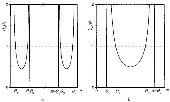
Figure 1: Effective potential $U_{eff}(\vartheta)$ as a function of $\vartheta$ for $\Lambda=-0.5,\ \mu=0.1$ (a), and $\Lambda=2,\ \mu=0$ (b).

The generalized momentum conjugated to the coordinate $\vartheta$ is the angular momentum component perpendicular to the plane passing through the $z$-axis and the Runge-Lenz vector $\bi{A}$ ($\mu=m/n$)

$$L_{\bot}(\vartheta)=n\sqrt{1+\frac{\Lambda}{1-5\sin^{2}\vartheta}-\frac{\mu^{2}}{\sin^{2}\vartheta}}=n\sqrt{1-U_{eff}(\vartheta)}.$$ (2.14)

Fig.1 shows the effective potential $U_{eff}(\vartheta)$ for two different cases: $\Lambda<0$ and $\Lambda>0$.

For negative values of $\Lambda$, the motion in intervals [$\vartheta_{1},\vartheta_{2}$] and [$\vartheta_{3},\vartheta_{4}$] is classically allowed (see Fig.1a), the value of $\Lambda$ is double degenerate and the final expression for the quantization rules has the form [12]

$$\int_{\vartheta_{1}}^{\vartheta_{2}}L_{\bot}(\vartheta)d\vartheta=\pi(s+1/2),$$

$$\int_{\vartheta_{3}}^{\vartheta_{4}}L_{\bot}(\vartheta)d\vartheta=\pi(s+1/2),\qquad s=0,1,2,...$$ (2.15)

Equations (2.15) give two degenerate states which are symmetric and antisymmetric to the $xy$ plane. In the case of $m=0$ the turning points $\vartheta_{1}$ and $\vartheta_{4}$ do not occur. Instead, the two singularities appear at $\vartheta=0,\pi$ due to the caustic at the $z$-axis which is characterized by the same Morse index as an ordinary turning point (see, e.g., [38] §49). Therefore, the quantization conditions in this case are formally obtained from the quantization conditions (2.15) by setting $\vartheta_{1}=0$ and $\vartheta_{4}=\pi$. The analysis of the roots of the function $L_{\bot}(\vartheta)$ shows that the states with $\Lambda<0$ exist only when $m<n/\sqrt{5}$.

When $\Lambda>0$, the region of a classically allowed motion is the interval [$\vartheta_{5},\vartheta_{6}$] (see Fig.1b). The $\Lambda$ values in this case are nondegenerate and are determined from the quantization condition [12]

$$\int_{\vartheta_{5}}^{\vartheta_{6}}L_{\bot}(\vartheta)d\vartheta=\pi(k+1/2),\qquad k=0,1,2,...$$ (2.16)

These states are localized outside the double cone $\Omega$ and their parity with respect to the $xy$ plane is equal to $(-1)^{k}$.

In the first (with respect to $\omega^{2}$) order of perturbation theory the quadratic Zeeman energy shifts are expressed in terms of the scaled value $\rho^{2}/n^{2}$ averaged over one period of the Kepler orbit

$$\varepsilon=\frac{<\rho^{2}>}{n^{2}}=\frac{1}{2}(1+\mu^{2}+\Lambda).$$ (2.17)

The $\Lambda$ values are determined by the quantization conditions (2.15) and (2.16). Of greatest interest are the outmost levels in a given $\{nm\}$-manifold, since they are the first to undergo overlap in the course of the approach to each other of two neighboring manifolds with increasing strength of the magnetic field. These energy levels correspond to the lowest levels in the effective potential $U_{eff}(\vartheta)$ in the quantization conditions (2.15) and (2.16). For these states the potential $U_{eff}(\vartheta)$ can be approximated by the harmonic oscillator and the scaled energy shift inside the cone $\Omega$ is ($\Lambda<0$)

$$\varepsilon_{osc.}=\sigma\sqrt{5+25\sigma^{2}}+\sqrt{5}\mu-5\sigma^{2}$$ (2.18)

and outside the cone $\Omega$ ($\Lambda>0$)

$$\varepsilon_{osc.}=\frac{5}{2}-\kappa\sqrt{5+\frac{25}{16}\kappa^{2}-\mu^{2}}+\frac{5}{4}\kappa^{2}-\frac{3}{2}\mu^{2}.$$ (2.19)

where $\sigma=(2s+1)/n$ and $\kappa=(2k+1)/n$. In Table 1 the scaled energy shifts (2.18) and (2.19) are compared with the quantum calculations. The quantum results have been obtained by diagonalisation of the energy matrix within the given {$nm$}-subspace. The agreement for the position of levels is very good for low-lying states. For higher states the agreement becomes less satisfactory since the applicability of harmonic oscillator approximation breaks down.

Table 1: Comparison of the quantum results $\varepsilon_{q}$ with the semiclassical approximation $\varepsilon_{osc.}$ (Eqs.(2.18) and (2.19)).

$n=40,\ m=0$ $s$ $\varepsilon_{q}$ $\varepsilon_{osc.}$ $k$ $\varepsilon_{q}$ $\varepsilon_{osc.}$ 0 0.055 0.053 0 2.45 2.44 1 0.159 0.142 4 2.03 2.06 2 0.255 0.212 8 1.65 1.75 3 0.342 0.267 12 1.32 1.51

$n=40,\ m=4$ $s$ $\varepsilon_{q}$ $\varepsilon_{osc.}$ $k$ $\varepsilon_{q}$ $\varepsilon_{osc.}$ 0 0.251 0.276 0 2.43 2.43 1 0.338 0.365 2 2.22 2.22 2 0.415 0.436 4 2.01 2.04 3 - - 6 1.82 1.88

With the increase of the magnetic field the first avoided crossing arises between the lowest-energy state $|1\rangle$ of the $n+1$ manifold and the highest-energy state $|2\rangle$ of the $n$ manifold. In the classical approach instead of avoided crossing we obtain the exact crossing of energy curves since the first ($\Lambda\simeq-1$) and the second ($\Lambda\simeq 4$) state are located in two nonoverlapping regions of configuration space (see Fig.1). The splitting is obtained in the quantum approach as the matrix element of diamagnetic potential between the first $|1\rangle$ and the second $|2\rangle$ state:

$$\Delta E=\langle 1|\omega\rho^{2}|2\rangle.$$ (2.20)

In the first order of quantum perturbation theory the Schrödinger equation is separable in elliptical-cylindrical coordinates on a sphere in a four-dimensional momentum space [11, 12, 13]. Using uniform semiclassical approximation for the wave functions of the states $|1\rangle$ and $|2\rangle$ in this coordinate system (see, e.g., [14]), the splitting is obtained in the form [12]

$$\Delta E\sim\exp\{-n\ln[(\sqrt{5}+2)(\sqrt{5}+1)/2]\}\simeq\exp(-1.92n),$$ (2.21)

which coincides with the probability of the under-barrier penetration in the effective potential $U_{eff}(\vartheta)$ with $\Lambda=-1$ in the interval $\vartheta\in[\vartheta_{2},\vartheta_{0}]$ (see Fig.1a), and with $\Lambda=4$ in the interval $\vartheta\in[\vartheta_{0},\vartheta_{5}]$ (see Fig.1b). Figure 2 demonstrates perfect agreement between this result and experimental data [10].

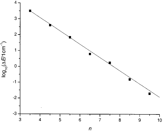
Figure 2: Energy splitting between the lowest-energy state of the $n+1$ manifold and the highest-energy state of the $n$ manifold as a function of principal quantum number $n$: solid line - the approximation (2.21), solid squared - experimental data from [10].

2.1.3 Helium atom; equivalent electrons

The first attempts to develop a semiclassical perturbation theory for a helium atom were made in the old Bohr theory (see, e.g., review [16]). According to heuristic concepts accepted at that time, only the simplest symmetric trajectories were considered, which is wrong from the modern point of view . The self-consistent perturbation theory was developed for equivalent electrons (having the same principal quantum number $n$) with total angular momentum equal to zero [17].

A distinguishing feature of the classical perturbation theory for equivalent electrons of a heliumlike system with the nuclear charge $Z$ is the presence of the accidental degeneracy in the unperturbed state. In this case, the perturbation series is the series over half-integer power of the small parameter $\lambda=1/Z$ (see [18] §108). To construct this series, first of all, the proper variables should be introduced. When the total angular momentum is equal to zero, the trajectories of the two electrons are on the same plane, regardless of the magnitude of the electron-electron interaction, and their angular momenta are equal but oppositely directed. In the zeroth order (without electron-electron interaction) both electrons move along the Kepler ellipses. The mutual orientation of the ellipses in the plane is specified by an angle $\vartheta=\vartheta_{1}-\vartheta_{2}$ with $\vartheta_{i}$ being the angle between the Runge-Lenze vector of the $i$-th electron and $z$-axis (see Fig.3). The position of the $i$-th electron on the ellipse is determined by the Kepler anomaly $\xi_{i}$ which is related to time by the relation

$$t-\tau_{i}=\frac{T_{i}}{2\pi}(\xi_{i}-\sqrt{1+2E_{i}L_{i}^{2}/Z^{2}}\sin{\xi_{i}})$$ (2.22)

where $\tau_{i}$ is the instant of passage through the perihelion, $E_{i}$ is the energy, $L_{i}$ is the angular momentum and $T_{i}$ is the period of the $i$-th electron. Since the dependence on time of the variables $\xi_{1}$ and $\xi_{2}$ is not independent, one of them (for the sake of definiteness $\xi=\xi_{1}$) and the time delay $\tau=\tau_{1}-\tau_{2}$ between the passage of the first and second electrons through the perihelion should be used.

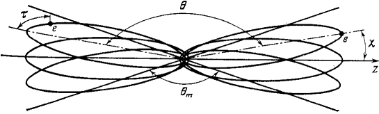
Figure 3: Trajectories of two equivalent electrons for the case $\chi_{m}=\pi/10$. From [17].

In the planar case (${\bi L}\equiv{\bi L}_{1}=-{\bi L}_{2}$), the motion of both electrons is described by eight Hamiltonian equations. It follows from four of them that the quantities ($L_{1}-L_{2}$) and ($\vartheta_{1}+\vartheta_{2}$) are exactly conserved, while ($E_{1}+E_{2}$) and ($\tau_{1}+\tau_{2}$) are conserved in the first-order. A nontrivial role is played by the equations

$$\frac{d\Delta E}{dt}=-\lambda\frac{\partial V}{\partial\tau},\ \ \frac{d\tau}{dt}=\frac{3}{E_{0}}\Delta E,$$ (2.23)

$$\frac{dL}{dt}=-\lambda\frac{\partial V}{\partial\vartheta},\ \ \frac{d\vartheta}{dt}=-\lambda\frac{\partial V}{\partial L},$$ (2.24)

where $E_{0}=-Z^{2}/2n$ is the unperturbed energy of one electron, $\Delta E=(E_{1}-E_{2})/2$ and $V(\xi,L,\vartheta,E_{1},E_{2},\tau)$ is the electron-electron Coulomb interaction. The small parameter $\lambda$ can be eliminated from equations (2.23) and (2.24) by changing from $\Delta E$ to $\varepsilon=\Delta E/\sqrt{\lambda}$ and introducing new ’times’ $s_{1}=\sqrt{\lambda}t$ and $s_{2}=\lambda t$ for the first and second pairs of the equations, respectively. It follows hence that the rate of change of $\tau$ and $\varepsilon$ is of the order of $\sqrt{\lambda}$, and that of $L$ and $\vartheta$ of the order of $\lambda$, i.e., the angular momentum $L$ and mutual angle $\vartheta$ vary infinitely slowly compared to time delay $\tau$ and scaled energy $\varepsilon$ as $\lambda\to 0$. In addition, the energy transfer $\Delta E$ is always small of the order of $\sqrt{\lambda}$, therefore the change of the parameters $E_{1}$ and $E_{2}$, as well as the periods in the electron-electron interaction should therefore be neglected, and these arguments of $V$ will hereafter be omitted. Since the characteristic frequencies are different, the motion along variables $\varepsilon,\tau$ and $L,\vartheta$ is adiabatically separated.

Most sensitive to electron-electron interaction are the variables $\varepsilon$ and $\tau$. They oscillate with period of the order of $\lambda^{-1/2}$, during which $L$ and $\vartheta$ can be regarded as constant. On the other hand, the oscillation over the Kepler anomaly $\xi$ has a high frequency compared to $\varepsilon$ and $\tau$. Replacing the interaction $V$ by its averaged value over common period ($T\equiv T_{1}=T_{2}$)

$${\cal V}(\tau;L,\vartheta)=\frac{1}{T}\int_{0}^{T}V(\xi(t),L,\vartheta,\tau)dt$$ (2.25)

we obtain one-dimensional problem in which $L$ and $\vartheta$ enter as parameters. The important feature of this one-dimensional problem is that only the ground state of the potential $\lambda{\cal V}(\tau;L,\vartheta)$ corresponds to the unperturbed state and for quantization the corresponding Schrödinger equation should be used. Since $\Delta E$ and $\tau$ are canonically conjugated variables, the Schrödinger equation reads

$$\Bigl{[}-\frac{3}{2E_{0}}\frac{d^{2}}{d\tau^{2}}+\lambda{\cal V}(\tau;L,\vartheta)\Bigr{]}\psi(\tau;L,\vartheta)={\cal E}(L,\tau)\psi(\tau;L,\vartheta)$$ (2.26)

with the periodic boundary condition: $\psi(0;L,\vartheta)=\psi(T;L,\vartheta)$. For all excited states of equation (2.26) $\Delta E$ is finite at $\lambda=0$ and they do not go over into the states of the unperturbed problem. In the first order of perturbation theory the wave function of the ground state is constant, which is $\psi_{0}=1/\sqrt{T}$. The first-order correction

$${\cal E}(L,\vartheta)=\int_{0}^{T}\psi_{0}^{2}(\tau){\cal V}(\tau;L,\vartheta)d\tau=\frac{1}{T}\int_{0}^{T}{\cal V}(\tau;L,\vartheta)d\tau$$ (2.27)

is additional integral of motion which is an effective Hamiltonian in the angle $\vartheta$. After the substitution of (2.25) into (2.27) this expression takes the form

$${\cal E}(L,\vartheta)=\frac{1}{T^{2}}\int_{0}^{T}\int_{0}^{T}\frac{dt_{1}dt_{2}}{|{\bi r}_{1}(t_{1})-{\bi r_{2}}(t_{2})|},$$ (2.28)

which coincides with classical averaging but for the nondegenerate case. This leads to the important conclusion that from the point of view of the quantization conditions there is no difference between the nondegenerate and accidental degenerate motion.

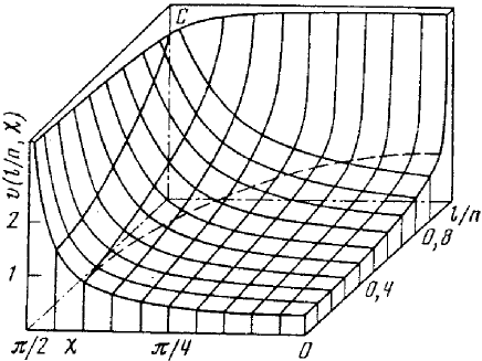
Figure 4: Effective Hamiltonian as a function of $\nu$ and $\chi$. The dashed line is the function $L(\chi)$ for $\chi_{m}=2\pi/5$ and $q=0.61$. From [17].

Using the explicit expression for the Kepler ellipses the scaling with respect to the principal quantum number $n$ is obtained

$${\cal E}(L,\vartheta)=\frac{Z}{n^{2}}v(\nu,\vartheta)$$ (2.29)

where $\nu=L/n$. The numerically calculated effective Hamiltonian $v(\chi,\nu)$ is shown in Fig.4.

The dependence of $L$ on $\vartheta$ is determined by the condition that ${\cal E}(L,\vartheta)$ is a constant on the trajectory, i.e.

$$v(\nu,\vartheta)=w$$ (2.30)

The constant $w$ is determined from the quantization condition, which (in terms of the variable $\chi=(\pi-\vartheta)/2$) is the same as considered for a hydrogen atom in a magnetic field at $m=0$ (see Sec.2.1.1). Finally, the quantization condition takes the scaled form

$$\int_{0}^{\chi_{m}}\nu(\chi)d\chi=\frac{\pi}{2}q$$ (2.31)

where $\chi_{m}$ is the turning point, $q=(2k+1)/2n$ and $k$ is a new quantum number $(k=0,1,2,...,n-1)$. In the first order, the correction $E^{(1)}$ to the unperturbed energy is equal to the average electron-electron interaction

$$E^{(1)}=\frac{Z}{n^{2}}w(q).$$ (2.32)

Figure 5 shows a plot of $w(q)$ and also the corrections, recalculated in accordance with the scaling rule (2.32), to the unperturbed energy in first-order quantum perturbation theory for helium and obtained by exact calculation for He and B³⁺ [17]. As it is seen, the agreement improves with increasing nuclear charge $Z$. The discrepancy between classical and quantum perturbation theory becomes noticeable only at $q>0.5$. It is attributable to the fact that as $q\to 1$ the turning point $\chi_{m}$ approaches the singular point $\chi=\pi/2$ (see Fig.4). In this case, the quantization condition (2.31) must be replaced by the modified quantization condition in which simultaneous account is taken of the turning point and the singular point at $\chi=\pi/2$.

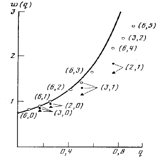
Figure 5: Scaled correction to the unperturbed energy: solid line - classical perturbation theory, open circles - quantum perturbation theory, solid triangles - exact values for He, solid circles - exact values for B³⁺. The parentheses contain the state quantum numbers ($n,k$). From [17].

2.2 Adiabatic switching method; hydrogen atom in external fields

The extension of the semiclassical quantization to the non-separable systems was proposed by Einstein in 1917 [21], who pointed out that the classical trajectory is Lagrangian manifold, so if the classical trajectory forms a torus in phase space, then in the $N$ dimensional problem only $N$ topologically independent quantization contours on this torus exist, and the actions along these contours are, according to the Liouville theorem, invariant with respect to the deformation of the contours. However, for a system with several degrees of freedom the calculation requires an excessive amount of computer time, mainly spent in rejecting unsuitable trajectories. To avoid this problem, the adiabatic switching method was proposed [20]. This method is based on the quantum Born-Fock adiabatic theorem [22] and the correspondence principle between quantum and classical mechanics. The adiabatic switching procedure is quite simple. To calculate energy spectrum of non-separable Hamiltonian $H$, first of all, we need to guess a reference Hamiltonian $H_{0}$ which is, on the one hand, solvable (separable) and, on the other hand, has the same topology of caustic as Hamiltonian $H$. Then one have to compute with the classical equations of motion the development in time of the initially quantized trajectory during a slow switching on the interaction $V=H-H_{0}$ ($H(\lambda)=H_{0}+\lambda(t)V$). When the interaction has been fully switched on ($\lambda=1$), the quantized trajectory for Hamiltonian $H$ and corresponding eigenvalue of energy are obtained, as well as, for all intermediate values of switching parameter $\lambda$. It is expected that the more slowly the interaction is switched on, the more precisely the quantization conditions are satisfied. Of course it is heuristic technics without proof but it works in many cases; it is a simple and effective tool to calculate the energy spectrum of involved multi-dimensional systems. The only thing necessary to control is that the topology of caustics does not change during the switching [20].

In the case of hydrogen atom in crossed electric $\bi F$ and magnetic $\bi B$ fields, the reference Hamiltonian $H_{0}$ is the Hamiltonian of the hydrogen atom [25]. Due to the high dynamical symmetry of the Coulomb interaction all trajectories in configuration space are closed lines - ellipses and just one quantization condition can be written which specifies principal quantum number $n$ only. When external perturbation is introduced, the trajectory fills up 3D domain in the configuration space and missed quantization conditions can be formulated. The perturbation theory for hydrogen atom in crossed electric and magnetic field is presented in Sec.2.1.1. Thus, the initial conditions for the quantized trajectory is determined by conditions (2.9). Next step is numerical calculation of classical equations for electron -

$$\frac{d^{2}{\bi r}}{dt^{2}}+\frac{\bi r}{r^{3}}=-\lambda(t)\Bigl{[}{\bi F}+\frac{1}{c}({\bi v}\times{\bi B})\Bigr{]}+\frac{1}{c}\frac{d\lambda(t)}{dt}{\bi A}$$ (2.33)

- during the switching external fields from $\lambda=0$ to the final values $\lambda=1$. In equation (2.33) $\bi A$ is the vector-potential (${\bi B}={\rm rot}{\bi A}$). The last term on right-hand side of equation (2.33) is the additional force arising as a consequence of the time dependence of the magnetic field. Although this force, being proportional to the switching rate, disappears in the adiabatic limit, it cannot be neglected. It ensures the adiabatic invariance, e.g., in the case of a pure magnetic field ($F=0$). Obviously, if it were neglected, the electron energy would be conserved exactly, that is wrong.

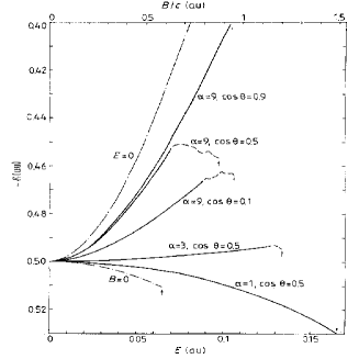
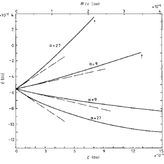
a)	b)

Figure 6: a) Ground state energy levels as functions of field strength for various combinations of parameters $\alpha=B/cE$ and $\cos\theta$. Chain curves are the quantum results for the cases of pure electric [27] and magnetic [26] fields. Broken curves demonstrate the non-adiabatic evolutions of the system. b) Energy levels of excited states, $(n,n_{1},n_{2})=(3,-1,-1)$ (the levels shifted downwards) and $(n,n_{1},n_{2})=(3,1,1)$ (the levels shifted upwards), as functions of field strength with constant parameters $\alpha=9,27$ and $\cos\theta=0.5$. Broken lines are the first-order perturbation theory results (2.10). The arrows indicate ionization in both figures. From [25].

Figure 6a shows the energy levels (full curves) of the ground state as a function of field strengths, for different combinations of parameters $\alpha=B/cF$ and the angle $\theta$ between $\bi F$ and $\bi B$. As a limit, quantum-mechanical results (chain curves) for the ground-state energies of a hydrogen atom in a magnetic field only ($E=0$) and in an electric field only ($B=0$) are shown. The curve labeled by $E=0$ is the result [26], obtained by diagonalising the energy matrix in an extensive basis of hydrogen wavefunctions. The curve labeled by $B=0$ is a quantum fourth-order perturbation theory result (see, for example, [27]). Figure 6b shows the results (full curves) for the states defined by the weak-field quantum numbers $(n,n_{1},n_{2})=(3,-1,-1)$ (the levels shifted downwards) and $(n,n_{1},n_{2})=(3,1,1)$ (the levels shifted upwards). The angle between the fields has been kept constant ($\cos\theta=0.5$) and the results are presented for two different ratios of field strengths: $\alpha=9$ and $\alpha=27$. Unlike the ground-state case, here the linear shift, given by (2.10) (broken lines), dominates in the limit of weak fields. The state (3,-1,-1) is bound stronger and the ionization limit was not reached in the range of fields shown in figure 6b. For the (3,1,1)-state the non-adiabatic behaviour was found only very close to the ionization limits. In Fig.6 electric field scale is common to all curves, while the magnetic field scale corresponds to curves labeled by $\alpha=9$ for the ground state and $\alpha=27$ for excited states. In all cases, the switching rate used in calculations was $d\lambda(t)/dt=2.5\times 10^{-5}$ au.

Again, adiabatic switching method has certain advantages with respect to the straightforward semiclassical quantization of non-integrable systems. It is free of such non-local problems as finding the caustics of the classical system and searching for the initial conditions which correspond to quantized trajectories (see, for example, [28]). In addition, this method provides all intermediate energy values at $0\leq\lambda\leq 1$.

2.3 Spontaneous decay of excited states of a hydrogen atom

A very interesting situation takes place in the problem of spontaneous decay of excited states of a hydrogen atom. From the classical point of view this process is due to the bremsstrahlung (see, e.g., [32, 33]). In the old Bohr quantum theory the bremsstrahlung was the main obstacle to the description of the stable atomic ground state within the framework of classical mechanics since the accelerating electron should emit radiation losing energy and finally should fall down onto the nucleus. However, it does not contradict the evolution of the excited states which are unstable.

According to classical electrodynamics, the rates of decrease of the energy $E(t)$ and the angular momentum $L(t)$ are described by the system of equations (see, e.g., [35] §75)

Table 2: Classical lifetime $\tau_{cl}$ (Eq.(2.35)) and quantum lifetime $\tau_{q}$ [34] for spontaneous decay of excited states of a hydrogen atom (in nanoseconds).

$nl$	2$p$	3$p$	4$p$	5$p$	6$p$	3$d$	4$d$	5$d$	6$d$	4$f$	5$f$	$6f$
$\tau_{cl}$	1.68	5.66	13.4	26.2	45.3	15.7	37.3	72.8	126	73.1	143	247
$\tau_{q}$	1.60	5.27	12.3	22.2	40.8	15.5	36.2	69.7	119	72.5	140	240

$$\frac{dE(t)}{dt}=-\frac{\{-2E(t)\}^{3/2}}{3c^{3}L(t)}\{3+2E(t)L^{2}(t)\},$$

$$\frac{dL(t)}{dt}=-\frac{2\{-2E(t)\}^{3/2}}{3c^{3}L^{2}(t)}.$$ (2.34)

The lifetime $\tau$ is defined by the expression $P=const\times\exp(-t/\tau)$, where $P$ is the population of the excited state. In classical mechanics there is no such concept, but we can estimate it as the time $\tau_{cl}$ in which the initial angular momentum decreases by unity ($\Delta L=1$), which corresponds to the emission of one photon. In the leading order of classical approach ($n,l\to\infty$) we can neglect the dependence on time in the right-hand side of equations (2.34). Then, after the substitution for the energy $E=-1/2n^{2}$ and angular momentum $L=(l+1/2)$ we obtain the following estimate of lifetime in terms of the quantum numbers $n,\ l$ [33]

$$\tau_{cl}=\frac{3}{2}c^{3}n^{3}(l+1/2)^{2}=9.32\times 10^{-11}n^{3}(l+1/2)^{2}\ \mathrm{sec}$$ (2.35)

In Table 2 these results for several states are presented in comparison with quantum calculations of total lifetimes $\tau_{q}$ of decay from the $nl$-state into all low-lying states [34]. This table demonstrates amazing agreement even for the low values of quantum numbers $n$ and $l$, though the lifetime is not well-defined in classical theory.

The system of equations (2.34) has an exact analytical solution but, according to the correspondence principle, only the leading classical order with respect to $n,l\to\infty$ has physical meaning. The next terms compete with unknown quantum corrections. Since the corrections of the same order caused by the different sources usually compensate each other, we obtain worse results taking them partly into account. It is the reason of bad agreement obtained in [32] where classical and quantum orders were mixed up.

Classical physics is deterministic, that is why the decay process has one channel providing the total lifetime only, and there is no way to analyze state-selective lifetime.

Generally, decay processes are not well-defined in quantum mechanics. Here we can not separate the quantum system from measurement. From the very beginning, it is formulated as a exponential decreasing in time of the population of state which is rather a classical treating of the problem. It is not clear how to determine the width of the energy level in the degenerated case, e.g., in the case of hydrogen atom in excited state at $n=2$. If we add weak spherical perturbation, the degeneracy is moved and correct wave functions are the spherical functions $|2s\rangle$ and $|2p\rangle$. Since the dipole matrix element between $|2s\rangle$ and ground state $|1s\rangle$ is equal to zero, $|2s\rangle$ is a meta-stable state having macroscopic lifetime - $1.4$ sec. The second state $|2p\rangle$ has typical atomic lifetime $1.6\times 10^{-9}$ sec. If we add weak electric field the correct wave functions are characterized by parabolic quantum numbers $n_{1},\ n_{2},\ m$ ($n=n_{1}+n_{2}+m+1$). At $n=2$ and $m=0$ there are two states $|nn_{1}n_{2}\rangle=|210\rangle$ and $|201\rangle$ which have the same lifetime of order $2.3\times 10^{-9}$ sec. But what is the lifetime for the hydrogen without any perturbation? There are huge difference between lifetime in spherical and parabolic coordinates. Here we have an unsolvable conflict with the superposition principle which is typical of classical processes.

2.4 Gutzwiller’s approach; broad resonances

The contribution of the unstable periodic orbit to the trace of the Green function is determined by the Gutzwiller formula [52]

$$g(E)\sim-\frac{iT(E)}{2\hbar}\sum_{n=1}^{\infty}\frac{\exp\{in[S(E)/\hbar-\lambda\pi/2]\}}{\sinh[nw(E)/2]}$$ (2.36)

where $S(E)$, $w(E)$, $T(E)$ and $\lambda$ are the action, the instability exponent, the period and the number of focal points during one period, respectively. After the expansion of the denominator, according to $[\sinh(x)]^{-1}=2e^{-x}\sum_{k=0}^{\infty}e^{-2kx}$, and summation of the geometric series over $n$ one can see that the response function (2.36) has poles at the complex energies $E_{ks}$ whenever

$$S(E_{ks})=\hbar\lambda\pi/2-i\hbar w(E_{ks})\left(k+\frac{1}{2}\right)+2s\pi\hbar,\ \ k,s=0,1,2,...$$ (2.37)

Equation (2.37) is a transcendental equation with respect to $E_{ks}$. This approach is not well-defined [1], but, in the case of the shortest period associated with unstable periodic orbit in separable system, the poles of (2.36) can be interpreted as manifestation of the resonances in the continuum. The width of these resonances is the linear function of $\hbar$ in spite of the under-barrier resonances whose width is exponentially small with respect to $\hbar\to 0$ ( $\propto e^{-2|S|/\hbar}$, where $S$ is under-barrier action). The Gutzwiller’s approach was applied to the realistic systems - the scattering of electron on Coulomb potential in the presence of magnetic [53, 54] and electric fields [55, 56], and scattering on two-Coulomb-center potential [56].

Table 3: Real parts $E_{G}$ and widths $\Gamma_{G}$ (in atomic units) for a sequence of resonances with parabolic quantum numbers $(n_{1},n_{2},m)$ at field strength $F=8$ kV/cm, as obtained from Gutzwiller’s approach (2.44). $E_{q}$ and $\Gamma_{q}$ are the results of the full quantum calculations [58].

$(n_{1},n_{2},m)$	(23,0,0)	(23,1,0)	(23,0,1)	(24,0,0)	(24,1,0)	(24,0,1)
$E_{G}\times 10^{4}$	1.899	1.774	2.597	3.360	3.251	4.021
$E_{q}\times 10^{4}$	1.949	2.039	2.698	3.382	3.433	4.090
$\Gamma_{G}\times 10^{4}$	0.499	1.480	1.145	0.632	1.887	1.355
$\Gamma_{q}\times 10^{4}$	0.524	1.681	1.188	0.638	1.955	1.369

As an example let us consider resonancees in elastic scattering of electron on the Coulomb centre in the uniform electric field $\bi F$ [56]. The Hamiltonian is separable in parabolic coordinates $u,v$ and $\varphi$ ($x^{2}+y^{2}=u^{2}v^{2}$, $2z=u^{2}-v^{2}$ and $u,v\geq 0$). After introducing a new time-like variable $\tau$ defined by the relation $d\tau=dt/(u^{2}+v^{2})$, the problem is reduced to two separated one-dimensional systems:

$$H_{1}=\frac{p_{u}^{2}}{2}+\frac{m^{2}\hbar^{2}}{2u^{2}}-Eu^{2}+\frac{1}{2}Fu^{4}=2\beta,$$ (2.38)

$$H_{2}=\frac{p_{v}^{2}}{2}+\frac{m^{2}\hbar^{2}}{2v^{2}}-Ev^{2}-\frac{1}{2}Fv^{4}=2(1-\beta),$$ (2.39)

where $\beta$ is a separation constant. At positive energy $E$ the motion in the coordinate $u$ is bounded whereas in the coordinate $v$ it is unbounded. The system (2.38),(2.39) has hyperbolic fixed point whose location in the $v-p_{v}$ space at energy $E=E_{ks}$ is given (up to first order in $\hbar$) by

$$v^{*}=\sqrt{|m|\hbar}(2E_{ks})^{-1/4}e^{i\pi/4},\ \ p_{v}^{*}=0,\ \ \beta^{*}=1+i|m|\hbar\sqrt{E_{ks}/2}$$ (2.40)

This fixed point corresponds to unstable state since in its vicinity the Hamiltonian $H_{2}$ has a form of turned oscillator ($\delta p_{v}=p_{v}-p_{v}^{*},\ \delta v=v-v^{*}$)

$$\delta^{2}H_{2}=\frac{1}{2}(\delta p_{v})^{2}-4E_{ks}(\delta v)^{2}.$$ (2.41)

In the first order with respect to $\hbar\to 0$ the corresponding action and instability exponent are

$$S(E_{ks})=2\int_{0}^{u_{0}}\sqrt{2E_{ks}u^{2}+4-Fu^{4}}du-|m|\pi\hbar-\frac{i}{2}|m|\hbar w(E_{ks}),$$ (2.42)

$$w(E_{ks})=4\sqrt{2E_{ks}}\int_{0}^{u_{0}}\frac{du}{\sqrt{2E_{ks}u^{2}+4-Fu^{4}}},$$ (2.43)

where $u_{0}$ is the external turning point. The substitution (2.42), (2.43) into (2.37) gives the transcendental equation for complex energy $E_{n_{1}n_{2}}$ ($s=n_{1}$, $k=n_{2}$, $\lambda=2$)

$$S(E_{n_{1}n_{2}})=(2n_{1}+1)\pi\hbar+i\hbar\Bigl{(}n_{2}+\frac{1}{2}\Bigr{)}w(E_{n_{1}n_{2}}).$$ (2.44)

which is, up to the first order of $\hbar$, equivalent with equations (15)-(17) in Ref.[57] obtained in quantum approach by the comparison equation method. Table 3 demonstrates a good agreement between Gutzwiller’s approach (2.44) and full quantum calculations [58] for the series of resonances which lie close to the real $E$-axis. They all correspond to large values of parabolic quantum number $n_{1}$ and small values of $n_{2}$ and $m$. The widths $\Gamma_{G}$ are comparable with the differences of the positions $E_{G}$ of the adjacent resonances. In this sense they can be referred to as ”broad resonances”. They explain, e.g., the experimentally observed resonant structure of photoionization cross section of the hydrogen atom near the ionization limit in strong electric fields [58, 59].

This problem was considered by Wintgen too [55]. His result, although qualitatively good, does not give correct values for the complex poles of expression (2.36) in the case $m=0$. The approach presented in [56] is based on the complex periodic orbits in the $m\neq 0$ case and gives the correct result for $m=0$ as $m\to 0$ limit.

The same approach with the same result was developed for broad resonances in the scattering of electron on two-Coulomb-center potential [56].

2.5 Poincaré section; resonances in helium atom

The Poincar$\acute{\mathrm{e}}$ section is a powerful tool to study the irregular motion in 2D non-separable problems because of the visualization of a dynamical system on one plot. In this case, the phase space is 4D with two coordinates $(x,y)$ and two momenta $(X,Y)$. At fixed energy $E$ one of these variables can be expressed from the equation $H(x,y,X,Y)=E$ as a function of the energy $E$ and the remained variables. Let it be, for instance, the second momentum $Y(x,y,X,E)$. Now if we plot on the plane $\{x,y\}$ the values of variables $x(t)=x_{i}$ and $X(t)=X_{i}$ each time $t_{i}$ when the coordinate $y(t)$ takes some value $y_{0}$ then, in the general case, the distribution of points ($x_{i},X_{i}$) in this plane is irregular. But if an additional integral of motion (may be approximate one) exists - $\Lambda(x,y,X,Y)$, then from the transcendental equation $\Lambda(x,y_{0},X,Y(x,y_{0},X,E))=\lambda$ we obtain the functional dependence of $x$ on $X$ and constants $y_{0}$, $E$ and $\lambda$: $x(X;y_{0},E,\lambda)$, where $\lambda$ is the value of the second integral of motion. As $t\to\infty$ ($i\to\infty$) the points ($x_{i},X_{i}$) from one trajectory fulfill this line. Calculation of many trajectories gives the Poincar$\acute{\mathrm{e}}$ section of the system, which visualizes the information about regular and irregular regions of motion. In the regular region there can exist two types of fixed points, elliptic and hyperbolic, associated with stable and unstable periodic orbits, respectively.

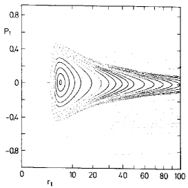
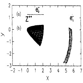
a)	b)

Figure 7: a) The Poincar$\acute{\mathrm{e}}$ section for collinear configurations of the electrons. The coordinate $r_{1}$ and the momentum $p_{1}$ of the outer electron is monitored whenever the inner electron approaches the nucleus ($r_{2}=0$). b) The periodic trajectory corresponding to the elliptic fixed point on the left panel (a) and a nonperiodic but regular trajectory in its neighbourhood (b). From [31].

Consider a collinear arrangement of a nucleus $Z$ and of two electrons, both being on the same side of the nucleus. It is a two-dimensional problem (position of inner and outer electrons on the axis), where we can use the Poincar$\acute{\mathrm{e}}$ section which is shown for helium in Figure 7a. In this section, the phase space position ($r_{1},\ p_{1}$) of the outer electron is monitored each time the inner electron approaches the nucleus ($r_{2}=0$). From Figure 7 one can see the elliptic fixed point at $p_{1}=0$ and $r_{1}\approx 7$, which corresponds to the two-electron periodic orbit (Fig.7b upper trajectory). Such a motion is a coherent oscillation of both electrons but with large difference in their positions and velocities. The outer electron appears to stay nearly frozen at large distance. This localization of outer electron is amazing since the total charge of the core (the nucleus and inner electron) is attractive. The existence of such states is explained by the resonant interchange of the energy between two electrons, i.e. it is a purely dynamical effect - at the conventional analysis we should expect that outer electron should fall down onto the nucleus since the total charge of nucleus and inner electron is equal to -1. Thus, it is very surprising that these classical configurations are extremely stable.

Semiclassical quantization near the periodic orbit is based on the Gutzwiller’s formula (2.36), but, since the orbit is stable, the instability exponent must be replaced by the stability parameter $\gamma=-iw$. The final expression of the quantized classical action of the tori surrounding the periodic orbit is given by [31]

$$S_{nkl}=s+1/2+2(k+1/2)\gamma_{1}+(l+1/2)\gamma_{2},\ \ \ \ \ s,k,l=0,1,2,...$$ (2.45)

where $\gamma_{1}=0.46164$ and $\gamma_{2}=0.06765$ the winding numbers, which describe the behaviour of nearby trajectories. The quantum numbers $s,\ k$ and $l$ reflect the approximate separability in the local coordinates parallel and perpendicular to the periodic orbit; $s$ is the quantum number along the periodic orbit, $k$ represents bending degree of freedom and $l$ corresponds to the perpendicular degree but preserving collinearity. Using the scaler property $S=S_{sc}/\sqrt{(}-2E)$, the quantized energy levels are obtained

$$E_{nkl}=-\frac{S_{sc}^{2}}{[s+1/2+2(k+1/2)\gamma_{1}+(l+1/2)\gamma_{2}]^{2}},$$ (2.46)

where $S_{sc}=1.4915$ is the (scaled) action of the periodic orbit for helium.

Table 4: Semiclassical energies $E_{scl}$ from expression (2.46), quantum energies $E_{q}$ and widths $\Gamma_{q}/2$ for the states of the series $(s,0,l))$. From [31].

$(s,k,l)$	(4,0,0)	(7,0,0)	(4,0,1)	(7,0,1)	(4,0,2)	(7,0,2)
$E_{scl}\times 10^{2}$	-8.91	-3.48	-8.68	-3.42	-8.45	-3.36
$E_{q}\times 10^{2}$	-8.96	-3.48	-8.76	-3.43	-8.61	-3.39
$\Gamma_{q}/2\times 10^{6}$	2.02	0.37	6.60	0.61	0.79	0.70

Table 4 shows the semiclassical energies (2.46) in comparison with full quantum calculation of energies $E_{q}$. In the table the width of the states $\Gamma_{q}$ with respect to the autoionization is also presented. One can see extremely small values of the widths for this series of asymmetric double excited states.

3 Ion-atom and electron-atom collisions

3.1 Electron-impact detachment of negative ion near the threshold

The ionization of a negative ion by an electron impact draws much attention because of a huge cross section. This reaction is very important, for instance, in understanding of stellar atmospheres.

First of all we need a classical description of the negative ion. The classical model for interaction of electron with neutral core of negative ion is based on the same physical assumptions as the zero-range potential model in the quantum theory [37], i.e. the potential well supporting one weakly bound $s$-state is spherical, narrow, and deep. The electron is oscillating along the diameter between the opposite turning points $d$ and $-d$. The frequency of this oscillation $\omega$ is the large parameter of the classical model. The bound $s$-state is represented by the ensemble of such trajectories uniformly distributed in all directions.

Now let us consider the detachment of the negative ion by an electron as a projectile. Near the threshold, because of the Coulomb repulsion between a negative ion and a projectile, there is another large parameter - the distance of the closest approach of the projectile to the negative ion $R_{0}$. Since $R_{0}$ is large, there is no interaction between the projectile and neutral core. Then, the equation of motion for the projectile is

$$\frac{d^{2}{\bi r}_{1}}{dt^{2}}=\frac{{\bi r}_{1}-{\bi r}_{2}}{|{\bi r}_{1}-{\bi r}_{2}|^{3}}$$ (3.1)

where ${\bi r}_{1}$ is the position vector of the projectile and ${\bi r}_{2}$ is the position vector of the bound electron. Since $r_{2}\leq d$, $r_{1}\geq R_{0}$ and $R_{0}\gg d$, we can expand the right-hand side of equation (3.1) over the multipole series. For our purposes, it is sufficient to consider the dipole approximation

$$\frac{d^{2}{\bi r}_{1}}{dt^{2}}=\frac{{\bi r}_{1}}{r_{1}^{3}}-\frac{{\bi r}_{2}}{r_{1}^{3}}+\frac{3({\bi r}_{1}\cdot{\bi r}_{2}){\bi r}_{1}}{r_{1}^{5}}$$ (3.2)

The first term on the right-hand side of equation (3.2) describes the interaction with the fixed Coulomb center, but the second and third represent the rapidly oscillating force with frequency $\omega$. Kapitsa developed an approximation method for this situation (see, e.g., [38], §30). In this method, the position vector of the projectile splits into two terms ${\bi r}_{1}=\bi{R}+\bi{r}$, where $\bi{R}$ is a smoothly-varying function and $\bi{r}$ is the rapidly oscillating part having zeroth mean value over a period $2\pi/\omega$. In the leading order with respect to $\omega\to\infty$ this method leads to the following results:

$$\frac{1}{2}\dot{R}^{2}+\frac{Eb^{2}}{R^{2}}+\frac{1}{R}=E,$$

$${\bi r}=\frac{1}{\omega^{2}}\Bigl{[}\frac{{\bi r}_{2}}{R^{3}}-3\frac{({\bi r}_{2}\cdot{\bi R}){\bi R}}{R^{3}}\Bigr{]},$$ (3.3)

where $b$ is the impact parameter and $E$ is the initial energy of the projectile. Ionization occurs when the work done by the projectile $A$ becomes equal to the binding energy of the negative ion $\epsilon$:

$$A\equiv\int\frac{({\bi r}_{1}-{{\bi r}_{2}})\cdot d{\bi r}_{2}}{|{\bi r}_{1}-{\bi r}_{2}|^{3}}=\epsilon$$ (3.4)

It is easily verified with the aid of (3.3) that the work done by a projectile is an oscillating function whose mean value is zero, and the amplitude of the oscillation increases in the course of the collision. Consequently, the energy necessary for ionization is not accumulated gradually in the collision process, but is transferred in a quarter of the period while the bound electron moves from the nucleus in the direction opposite to that of the projectile. The orientation of each trajectory in the ensemble is characterized by spherical angles $\vartheta$, $\varphi$ with respect to the vector ${\bi R}(t)$. The classical trajectories, for which escape is possible, are then restricted to a cone $\Omega(t)$ with $\vartheta\leq\vartheta_{m}(t)$. The size of the cone is obtained from (3.4):

$$\frac{d\cos\vartheta_{m}(t)}{R^{2}(t)}=\epsilon.$$ (3.5)

The detailed analysis shows that the cone corresponding to the distance of the closest approach $\Omega_{0}$ absorbs all previous cones $\Omega(t)$. Therefore, the probability of ionization at a given impact parameter $b$ is

$$W(b)=\frac{1}{2\pi}\int_{\Omega_{0}}\sin\vartheta d\vartheta d\varphi=1-\frac{E_{th}^{2}}{4E^{2}}(1+\sqrt{1+4E^{2}b^{2}})^{2}$$ (3.6)

where $E_{th}=\sqrt{\epsilon/d}$ is the classical threshold of detachment. The normalization factor in equation (3.6) is taken as $1/2\pi$ because the opposite directions represent the same trajectory. The total detachment cross section is [39]

$$\sigma=2\pi\int_{0}^{b_{m}}W(b)bdb=\frac{\pi}{2E_{th}^{2}E^{4}}(E-E_{th})^{2}\Bigl{(}E^{2}+\frac{2}{3}EE_{th}+\frac{1}{3}E_{th}^{2}\Bigr{)},$$ (3.7)

where $b_{m}=\sqrt{E(E-E_{th})}/(E_{th}E)$. The classical threshold energy $E_{th}$ differs from the quantum threshold energy $\epsilon$, because, in the classical approach, the projectile needs extra energy to overcome the Coulomb repulsion and to reach the distance where ionization occurs. For $\epsilon<E<E_{th}$ the detachment mechanism is purely quantum, it is an the underbarrier penetration.

Figure 8 shows the cross section (3.7) for electron-impact detachment of H^- (or D^-) in comparison with experimental data. The parameters for H^- were taken from [37]: $d=2.7$ and $\epsilon=0.0278$. The classical results are in good agreement with experimental data [45] and follow the shape of experimental data [46] in the threshold region. However, they are shifted approximately by 2 eV with respect to the latter. This shift is equal to the difference between classical (2.76 eV) and quantum (0.76 eV) thresholds.

It is not clear how to reproduce the classical mechanism of detachment in quantum mechanics. The detachment cross section in the threshold region depends critically on the interaction between the projectile and the rapidly oscillating bound electron. In quantum mechanics, it is difficult to take this interaction into account rigorously, whereas in classical approach this can be done simply and naturally. In [40] the authors tried to modify the classical approach. However, the proposed ”corrections” are beyond the selfconsistent asymptotic approach. For instance, it was taken into account that not all electrons, satisfying the condition $\vartheta<\vartheta_{m}$, have time to leave the negative ion during collision, and, at the same time, the under barrier penetration is considered, in fact, as an instant process.

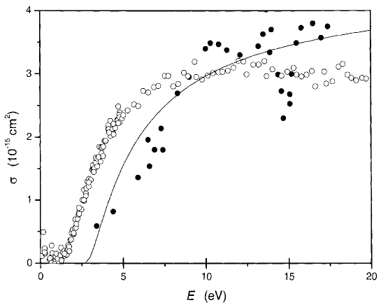
Figure 8: The detachment cross section of H^- (or D^-) as a function of electron impact energy. The full curve is the classical cross section (3.7), the open circles are experimental data from [45] and the solid circles are experimental data from [46].

3.2 Non-adiabatic transitions via hidden crossings

In slow atomic collisions the inelastic transitions between electronic adiabatic states occur at the place of the closest approach of adiabatic potential curves - avoided crossings. Initially in the application of the adiabatic approach the narrow avoided crossings due to the under-barrier resonant interaction of two electronic states located on different nuclei were used. Later [42] the new mechanism of nonadiabatic transitions via the so-called ’hidden crossings’ were discovered. Hidden crossings happen when an electronic energy level touches the top of an effective potential. In the classical description the full dimensional electronic trajectory collapses into an unstable periodic orbit at this place. The transitions via hidden crossings are dominant in atomic collisions. They provide a complete description of inelastic processes in atomic collisions. The classical/semiclassical theory of hidden crossings was developed in [43]. In detail it is discussed in the review paper [44].

3.3 Binary encounter approximation

For inelastic transitions of atomic electron in the charged projectile-neutral atom collisions, the binary encounter approximation can be applied. This approximation is based on the assumption that inelastic cross sections can be obtained from the two-body (projectile-atomic electron) elastic cross section after averaging over the momentum distribution of atomic electron in the initial atomic state. This scheme can be used in both quantum and classical approach.

Initially, the classical binary encounter approximation was developed for fast collisions (see, e.g., review paper [47] and references therein). In [49], the restriction on impact velocity $v_{p}>>v_{e}$, where ${\bi v}_{p}$ and ${\bi v}_{e}$ are the initial projectile and atomic electron velocities, was removed. The most interesting case is the case when the projectile is an electron. In this case, the electro-electron velocity transfer from the projectile to the atomic electron is given by

$$\Delta{\bi v}_{e}=\frac{2(v^{3}{\bi b}-2{\bi v})}{{v^{4}b}^{2}+4},$$ (3.8)

where ${\bi v}={\bi v}_{p}-{\bi v}_{e}$ is the electron-electron impact velocity and $\bi b$ is a vector of impact parameter (${\bi v}\bot{\bi b}$). Then the kinetic energy transfer is

$$\Delta E({\bi b})=\frac{2v_{p}v_{e}v^{2}b\sin\vartheta\cos\chi+2v^{2}+4({\bi v}\cdot{\bi v}_{e})}{v^{4}b^{2}+4},$$ (3.9)

where $\vartheta$ is the angle between ${\bi v}_{p}$ and ${\bi v}_{e}$, $\chi$ is the angle between vector of ${\bi b}$ and the plane in which vectors ${\bi v}_{p}$ and ${\bi v}_{e}$ lie. The boundary of the region of $\bi b$ values which lead to an energy transfer greater than $\varepsilon$ is specified by the condition $\Delta E({\bi b})=\varepsilon$, and the differential cross section with respect to velocities of projectile ${\bi v}_{p}$ and atomic electron ${\bi v}_{e}$ for the transfer of an energy $\Delta E({\bi b})\geq\varepsilon$ is

$$\Sigma({\bi v}_{p},{\bi v}_{e},\varepsilon)=\int\Theta(\Delta E({\bi b})-\varepsilon)d^{2}{\bi b}=\frac{\pi}{v^{4}\varepsilon^{2}}({v^{\prime}}_{p}^{2}{v^{\prime}}_{e}^{2}-v_{p}^{2}v_{e}^{2}\cos^{2}\vartheta),$$ (3.10)

where $\Theta(x)$ is the step-wise Heaviside function, and ${v^{\prime}}_{p}=\sqrt{v_{p}^{2}-2\varepsilon}$, ${v^{\prime}}_{e}=\sqrt{v_{e}^{2}+2\varepsilon}$ are the projectile and atomic electron velocities in the final state. Assuming the isotropic distribution over ${\bi v}_{e}$ in the initial atomic state the averaged cross section is obtained as

$$\Sigma(v_{p},v_{e},\varepsilon)=\frac{\pi}{8\varepsilon^{2}}\cases{\frac{v_{p}^{2}+v_{e}^{2}}{v_{p}v_{e}}\ln{\frac{(v_{p}+v_{e})^{2}}{(v_{p}-v_{e})^{2}}}-2\frac{({v^{\prime}}_{p}^{2}-{v^{\prime}}_{e}^{2})^{2}}{({v}_{p}^{2}-{v}_{e}^{2})^{2}}-2&$v_{p}\geq{v^{\prime}}_{e}$,\cr\frac{v_{p}^{2}+v_{e}^{2}}{{v^{\prime}}_{p}{v^{\prime}}_{e}}\ln{\frac{(v_{p}^{2}+v_{e}^{2}+2{v^{\prime}}_{p}{v^{\prime}}_{e})}{(v_{p}^{2}+v_{e}^{2}-2{v^{\prime}}_{p}{v^{\prime}}_{e})}}-4&$v_{p}<{v^{\prime}}_{e}$.\cr}$$ (3.11)

The final expression for the cross section $\sigma(v_{p},\varepsilon)$ is found by taking an average of (3.11) over the distribution of electron in the atom $q({\bi r})$. For the spherical symmetric atomic potential $V(r)$ the distribution in the ${nl}$-subshell has the form [48]

$$q_{nl}({\bi r})=\frac{1}{2\pi r^{2}T_{nl}p_{nl}(r)},$$ (3.12)

where $p_{nl}(r)=\sqrt{2[E_{nl}-V(r)-L^{2}/2r^{2}]}$ is the radial momentum of atomic electron in the initial state $E_{nl}$, $L=\hbar(l+1/2)$ and $T_{nl}$ is the period of oscillation over $r$. Then the cross section is expressed as an integral between the turning points $r_{1,2}$

$$\sigma_{nl}(v_{p},\varepsilon)=\frac{2}{T_{nl}}\int_{r_{1}}^{r_{2}}\Sigma(v_{p},\sqrt{2[E_{nl}-V(r)]},\varepsilon)\frac{dr}{p_{nl}(r)}.$$ (3.13)

For the fast collision ($v_{p}\to\infty$), the cross section does not depend on the mass of projectile and has a general asymptote

$$\sigma_{nl}(v_{p},\varepsilon)=\frac{2\pi Z^{2}}{3v_{p}^{2}\varepsilon^{2}}[3\varepsilon+2(E_{nl}-\tilde{V}_{nl})],$$ (3.14)

where $\tilde{V}_{nl}$ is the average potential energy (for Coulomb potential $\tilde{V}_{nl}=2E_{nl}$) and $Z$ is the charge of the projectile. At $\varepsilon=|E_{nl}|$ expressions (3.13),(3.14) give the ionization cross section $\sigma_{ion}(v_{p})$.

To calculate the cross section for excitation to a state with a principal quantum number $n^{\prime}$, $\varepsilon$ in (3.12) should be presented in the form $\varepsilon=E_{n^{\prime}}-E_{nl}$ and then after differentiation of (3.12) with respect to $n^{\prime}$ the cross section of excitation is obtained [49]

$$\sigma_{nl\to n^{\prime}}(v_{p})=\Bigl{|}\frac{\partial\sigma_{nl}(v_{p},\varepsilon)}{\partial\varepsilon}\frac{dE_{n^{\prime}}}{dn^{\prime}}\Bigr{|}_{\varepsilon=E_{n^{\prime}}-E_{nl}}=$$

$$=\frac{4\pi}{T_{n^{\prime}}T_{nl}}\Biggl{|}\int_{r_{1}}^{r_{2}}\frac{\partial\Sigma(v_{p},\sqrt{2[E_{nl}-V(r)]},\varepsilon)}{\partial\varepsilon}\frac{dr}{p_{nl}(r)}\Biggr{|}_{\varepsilon=E_{n^{\prime}}-E_{nl}},$$ (3.15)

where $T_{n^{\prime}}$ is the period of oscillation over $r$ in the final state $n^{\prime}$. In (3.15) the fact was used that in the semiclassical approximation the derivative of the energy with respect to the quantum number is equal to the classical frequency: $dE_{n^{\prime}}/dn^{\prime}=2\pi/T^{\prime}$ which follows straightforwardly from the Bohr-Sommerfeld quantization condition.

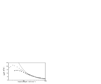
a)	b)

Figure 9: a) The ionization cross section of He(${}^{3}S$) metastable as a function of electron impact energy. The full curve is the classical cross section (3.13) and the solid circles are experimental data [50]. b) The ionization cross section of hydrogen atom by proton and He²⁺ as a function of scaled impact energy. The full curve is the asymptote (3.14), the solid and open circles are the experimental data [51] for proton and He²⁺ as a projectile.

Figure 9a shows the cross section for electron-impact ionization of helium in the meta-stable state He(2${}^{3}S$). It can be seen that classical expressions give good agreement with experimental results in the whole range of impact energy. In Fig.9b the comparison of asymptote (3.14) with experimental data for ionization of hydrogen atom by proton and He²⁺ is presented. The discrepancy at very high impact velocity in both figures is explained by logarithmic-like dependence of the cross section ($\sigma\propto\ln v_{p}/v_{p}^{2}$) due to the contribution from individual dipole transition. However, according to Ehrenfest’s theorem, the classical description deals with the wavepackets. In order to obtain a wavepacket, which imitates the motion of a classical particle, one needs to perform integration over the quantum numbers in a narrow range. As a result of this averaging, the logarithmic energy dependence disappears. It explains the absence of the logarithmic energy term in the classical cross sections.

To calculate the state selective excitation $nl\to n^{\prime}l^{\prime}$, the angular-momentum transfer is needed. The square of the angular momentum in the final state can be written

$$L^{\prime 2}=[{\bi r}\times({\bi p}+\Delta{\bi p})]^{2}=L^{2}+r^{2}(2p_{\perp}\Delta p_{\perp}\cos\alpha+\Delta p_{\perp}^{2}),$$ (3.16)

where ${\bi p}_{\perp}$ and $\Delta{\bi p}_{\perp}$ are the projections of ${\bi p}$ and $\Delta{\bi p}$ onto the plane perpendicular to $\bi r$, and $\alpha$ is the angle between ${\bi p}_{\perp}$ and $\Delta{\bi p}_{\perp}$. Since for transition from the $(nl)$-subshell the initial distribution $q_{nl}({\bi r})$ is isotropic, the distribution with respect to $L^{\prime}$ for fixed values of $\bi r$ and $\bi b$ is

$$\lambda({\bi r},{\bi b},L^{\prime})=\frac{1}{2\pi}\Bigl{|}\frac{d\alpha}{dL^{\prime}}\Bigr{|}=\frac{2L^{\prime}}{\pi r^{2}\sqrt{(\mu_{2}^{2}-\Delta p^{2}_{\perp})(\Delta p_{\perp}^{2}-\mu_{1}^{2})}},$$ (3.17)

where $\mu_{1,2}=(L^{\prime}\pm L)/r$. After averaging of (3.17) over the impact parameter $\bi b$ and the initial distribution $q_{nl}({\bi r})$ the final result is obtained as a single radial integral over the classically allowed region which is common to the initial and final states. The detailed analysis of this cross section can be found in [48, 49]. In the case $n,n^{\prime}\gg\Delta n$ and $L,L^{\prime}\gg\Delta L$ ($\Delta n=|n^{\prime}-n|,\ \Delta L=|L^{\prime}-L|$) in high-energy limit the cross section has the form

$$\sigma_{nl\to n^{\prime}l^{\prime}}(v_{p})=\frac{32n^{3}(n^{2}-L^{2})^{3/2}}{9\pi v_{p}^{2}(n\Delta n^{2}+n\Delta L^{2}-2L\Delta n\Delta L)^{2}}$$ (3.18)

This expression reveals some important features. For fixed values of $n$ and $L$, the cross section sharply decreases with increasing $\Delta n$ and $\Delta L$, as $(\Delta n)^{-4}$ and $(\Delta L)^{-4}$.

4 Classical representation in quantum mechanics

At first sight, the classical representation is impossible in quantum theory, for instance, because of tunneling phenomenon, which is, at first sight, incompatible with the classical approach. However, if we consider a particle scattered by a parabolic barrier, we find that, on the one hand, there is an effect of sub-barrier penetration and, on the other hand, the time-dependent Green function, which carries full information about the quantum system, is exactly expressed in terms of the classical action along classically allowed trajectories only. Thus, in principle, the tunneling effect could be explained in terms of classical trajectories.

4.1 Abel transform to the classical representation

For the sake of transparency we consider a symmetric potential $V(x)=V(-x)$, where $V(0)=0$ and $V(x)$ increases monotonically to infinity on the semiaxis $x>0$. To introduce the classical representation the linear equation for the quantum probability density $\rho_{n}(x)=\psi_{n}^{2}(x)$ is needed , which is obtained from the Schrödinger equation [61]

$$-\frac{\hbar^{2}}{4m}\frac{d^{3}\rho_{n}(x)}{dx^{3}}+2[V(x)-E_{n}]\frac{d\rho_{n}(x)}{dx}+\frac{dV(x)}{dx}\rho_{n}(x)=0.$$ (4.1)

This third-order differential equation has three linearly independent solutions - two of these are related to the Schrödinger equation and the third to the solution of the Milne equation having the meaning of the quantum wavelength (see Sec.5).

Now let us represent the quantum state $n$ as an ensemble of classical states in the potential $V(x)$ distributed in the energy $\epsilon$ with a certain probability density $\phi_{n}(\epsilon)$

$$\rho_{n}(x)=\int_{V(x)}^{\infty}q(\epsilon,x)\phi_{n}(\epsilon)d\epsilon,$$ (4.2)

where

$$q(\epsilon,x)=\frac{\sqrt{2m}}{T(\epsilon)\sqrt{\epsilon-V(x)}}$$ (4.3)

is the $x$-distribution for the classical state at given energy $\epsilon$ and $T(\epsilon)$ is a classical period. A remarkable property of the representation (4.2) is its reciprocity. This becomes evident if instead of $x$ the potential $V$ is taken as an independent variable. Such a change of variable is standard in classical mechanics and reduces the conversion of expression (4.2) to the well-known Abel problem, whence

$$\phi_{n}(\epsilon)=-\frac{T(\epsilon)}{\pi\sqrt{2m}}\int_{\epsilon}^{\infty}\frac{1}{\sqrt{V-\epsilon}}\frac{d\rho_{n}(x(V))}{dV}dV,$$ (4.4)

where $x(V)$ is the inverse of function $V(x)$.

The transforms (4.2), (4.4) are an analogue of the Fourier transform connecting configuration and momentum representations and it is called ’a classical representation’, since the kernel $q(\epsilon,x)$ is the classical probability density and $\phi(\epsilon)$ has the meaning of the energy distribution in the classical ensemble.

In the classical representation, the Schrödinger equation (4.1) transforms into an equation for scaled energy distribution $\tilde{\phi}_{n}(\epsilon)=\phi_{n}(\epsilon)/T(\epsilon)$:

$$(\epsilon-E_{n})\tilde{\phi}_{n}(\epsilon)=\frac{\hbar^{2}}{m}\int_{\epsilon}^{\infty}Q(\mu,\epsilon)\frac{d^{3}\tilde{\phi}_{n}(\mu)}{d\mu^{3}}d\mu,$$ (4.5)

with the kernel

$$Q(\mu,\epsilon)=\frac{1}{15\pi}\int_{x_{1}}^{x_{2}}\frac{1}{\sqrt{V(x)-\epsilon}}\frac{d^{3}(\mu-V(x))^{5/2}}{dx^{3}}dx,$$ (4.6)

where $x_{1}$ and $x_{2}$ are the turning points defined by the conditions: $V(x_{1})=\epsilon$ and $V(x_{2})=\mu$. The discrete spectrum $E_{n}$ is obtained from the boundary condition: $\tilde{\phi}_{n}(\epsilon)\to 0$ as $\epsilon\to\infty$. Equation (4.5) looks like a balance equation for ’virtual’ transitions between the classical states with the energies $\epsilon$ and $\mu$. It is very interesting to extract the probability of such transitions from equation (4.5).

The energy distribution $\phi_{n}(\epsilon)$ obeys the obvious normalization condition

$$\int_{0}^{\infty}\phi_{n}(\epsilon)d\epsilon=1$$ (4.7)

In addition to this, the general condition holds

$$\int_{0}^{\infty}\epsilon\phi_{n}(\epsilon)d\epsilon=E_{n},$$ (4.8)

which is not trivial and means that the average energy of classical ensemble is equal to the eigen-energy of quantum state $|n\rangle$.

4.2 Harmonic oscillator

Let us consider the harmonic-oscillator problem

$$V(x)=\frac{1}{2}m\omega^{2}x^{2}$$ (4.9)

as an example in which the classical representation is employed. In this case the kernel can be calculated explicitly:

$$Q(\mu,\epsilon)=\frac{1}{4}m\omega^{2}(\mu-2\epsilon).$$ (4.10)

Substituting this into (4.5) yields an equation for harmonic oscillator in classical representation

$$\frac{\hbar^{2}\omega^{2}}{4}\Bigl{[}\epsilon\frac{d^{2}\phi_{n}(\epsilon)}{d\epsilon^{2}}+\frac{d\phi_{n}(\epsilon)}{d\epsilon}\Bigr{]}+(E_{n}-\epsilon)\phi_{n}(\epsilon)=0,$$ (4.11)

which formally coincides with the radial Schrödinger equation for the Sturmian basis functions of the hydrogen atom with the negative ’angular quantum number’ $l=-1/2$. In the Sturmian approach the energy is fixed and the charge is quantized. The energy $E_{n}$ plays the role of the ’charge’ in this ’hydrogen Schrödinger equation’, its spectrum is $E_{n}=\hbar\omega(n+1/2)$, and the corresponding energy distribution reads

$$\phi_{n}(\epsilon)=\frac{2}{\hbar\omega}e^{-2\epsilon/\hbar\omega}L_{n}(4\epsilon/\hbar\omega),$$ (4.12)

where $L_{n}(x)$ is a Laguerre polynomial.

4.3 Inelastic transitions in the Feynman model

As practical application of the classical representation, the problem of description of the initial and final states in classical trajectory Monte Carlo (CTMC) method [62] in the theory of atomic collisions is the first candidate. In this method the initial state of the electron is specified as an ensemble of classical states with the energy equal to the energy $E_{n}$ of the corresponding atomic state. Then the evolution of this ensemble is calculated according to the classical equations of motion. The main difficulty in this approach is to extract the contribution of different quantum states in the final ensemble as $t\to\infty$, since the final energies of classical trajectories assume continuous values that do not coincide with the atomic spectrum. On the other hand, the classical representation (4.4) provides the exact description of quantum states in terms of an ensemble of classical trajectories. This fact can be used to modify the CTMC method in the treatment of the initial and final states. Of course, the solution of the dynamical problem remains classical, i.e. approximate. To illustrate such an approach, let us consider inelastic transitions in the Feynman model [63] with the nonstationary potential

$$V(x,t)=\frac{1}{2}m\omega^{2}x^{2}+\alpha(t)x,$$ (4.13)

where $\alpha(t)$ is the strength of a homogeneous external field that is time-dependent and tends to zero as $t\to\pm\infty$. In this case, the general solution of the classical equation of motion can be obtained explicitly

$$x(t)=\frac{1}{m\omega}\int_{-\infty}^{t}\alpha(t^{\prime})\sin\omega(t-t^{\prime})dt^{\prime}+\frac{\sqrt{2\epsilon}}{\omega}\sin{\omega(t-\tau)},$$ (4.14)

where $\epsilon$ and $\tau$ are the initial energy and phase. As $t\to+\infty$ this solution describes harmonic oscillation with an energy

$$\mu=\epsilon+\nu+2\sqrt{\epsilon\nu}\cos{\tau},$$ (4.15)

where

$$\nu=\frac{1}{2m^{2}}\Bigl{|}\int_{-\infty}^{+\infty}\alpha(t)e^{i\omega t}dt\Bigr{|}^{2}.$$ (4.16)

Since the distribution over the initial phase is uniform, the energy distribution in the final state at initial energy $\epsilon$ has the form

$$p(\mu,\epsilon)=\frac{1}{\pi}\frac{d\tau}{d\mu}=\frac{\theta(\mu-\mu_{1})\theta(\mu_{2}-\mu)}{\pi\sqrt{\theta(\mu-\mu_{1})\theta(\mu_{2}-\mu)}},$$ (4.17)

where $\mu_{1}=(\sqrt{\epsilon}-\sqrt{\nu})^{2}$, $\mu_{2}=(\sqrt{\epsilon}+\sqrt{\nu})^{2}$ and $\theta(x)$ is the unite step-function. Then the probability of an inelastic transition from the state $|n\rangle$ to the state $|k\rangle$ is [61]

$$P_{nk}(\gamma)=\int_{0}^{\infty}d\mu\phi_{k}(\mu)\int_{\epsilon_{1}}^{\epsilon_{2}}d\epsilon p(\mu,\epsilon)\phi_{n}(\epsilon)=L_{n}^{k-n}(\gamma)L_{k}^{n-k}(\gamma))e^{\gamma},$$ (4.18)

where $\phi_{k}(\mu)$ and $\phi_{n}(\epsilon)$ are the energy distributions of the initial and final states defined by (4.12), $\epsilon_{1}=(\sqrt{\mu}-\sqrt{\nu})^{2}$, $\epsilon_{2}=(\sqrt{\mu}+\sqrt{\nu})^{2}$, $\gamma=\nu/\hbar\omega$ and $L_{p}^{q}(x)$ is a generalized Laguerre polynomial. The probability (4.18) coincides with the exact quantum expression (see [63]), although the classical solution (4.14) is approximate from a quantum point of view.

4.4 Semiclassical approach

The rough classical approximation is obtained if we neglect the right-hand side in equation (4.5). Then $\phi_{n}(\epsilon)=\delta(\epsilon-E_{n})$ and from (4.2) the density of probability takes the form

$$\rho_{n}(x)=\frac{\sqrt{2m}}{T(E_{n})\sqrt{E_{n}-V(x)}}.$$ (4.19)

However, the solution $\tilde{\phi}_{n}(\epsilon)$ as well as $\rho_{n}(x)$ has essential singularity as $\hbar\to 0$:

$$\tilde{\phi}_{n}(\epsilon)\propto\sin\Bigl{(}\frac{1}{\hbar}W(\epsilon)\Bigr{)}.$$ (4.20)

To construct semiclassical approximation, the integral in the right-hand side of equation (4.5) has to be integrated by parts twice

$$(\epsilon-E_{n})\tilde{\phi}_{n}(\epsilon)=\frac{\hbar^{2}}{8m}\Bigl{[}\frac{dV(x)}{dx}\Bigl{|}_{V=\epsilon}\Bigr{]}^{2}\frac{d^{2}\tilde{\phi}_{n}(\epsilon)}{d\epsilon^{2}}+$$

$$+\frac{\hbar^{2}}{m}\frac{d^{2}V(x)}{dx^{2}}\Bigl{|}_{V=\epsilon}\frac{d\tilde{\phi}_{n}(\epsilon)}{d\epsilon}+\frac{\hbar^{2}}{m}\int_{\epsilon}^{\infty}\frac{d^{2}Q(\mu,\epsilon)}{d\mu^{2}}\frac{d\tilde{\phi}_{n}(\mu)}{d\mu}d\mu.$$ (4.21)

Here the coefficients in front of the second and first derivatives of $\tilde{\phi}_{n}(\epsilon)$ are obtained from definition of $Q(\mu,\epsilon)$ (4.6). Since $\tilde{\phi}_{n}(\epsilon)$ has essential singularity with respect to $\hbar$, in zero order only the first term in the right-hand side should be retained. Then $W(\epsilon)$ takes the form

$$W(\epsilon)=2\int^{\epsilon}\sqrt{2m(E_{n}-\epsilon^{\prime})}\Bigl{[}\frac{dV(x)}{dx}\Bigl{|}_{V=\epsilon^{\prime}}\Bigr{]}^{-1}d\epsilon^{\prime}.$$ (4.22)

After substitution (4.20) with $W(\epsilon)$ (4.22) into expression (4.2), the density of probability can be estimated by the expression

$$\rho(x)\propto\int^{\infty}_{V(x)}q(\epsilon,x)\sin\Bigl{(}\frac{2}{\hbar}\int^{\epsilon}\sqrt{2m(E_{n}-\epsilon^{\prime})}\Bigl{[}\frac{dV(x)}{dx}\Bigl{|}_{V=\epsilon^{\prime}}\Bigr{]}^{-1}d\epsilon^{\prime}\Bigr{)}d\epsilon.$$ (4.23)

Semiclassical expansion of $\rho(x)$ is generated by consecutive integration by parts in (4.23). In the leading order

$$\rho(x)\propto\cos\Bigl{(}\frac{2}{\hbar}\int^{x}\sqrt{2m(E_{n}-V(x^{\prime}))}dx^{\prime}\Bigr{)}=$$

$$=2\cos^{2}\Bigl{(}\frac{1}{\hbar}\int^{x}\sqrt{2m(E_{n}-V(x^{\prime}))}dx^{\prime}/\hbar\Bigr{)}-1.$$ (4.24)

The last term, -1, has to be omitted because it is beyond the semiclassical series, and the result coincides with the well-known semiclassical expansion of $\rho(x)$ in the leading order.

4.5 Scattering problem; tunneling phenomenon

In quantum mechanics, the scattering problem is out of Hilbert space and we have no well-defined physical stationary states because of normalization problem. It is a very serious defect of the theory. Below the boundary of the continuum, the aim of the theory is the search for stable (or stationary) states which exist at discrete energy values only. Above the boundary of the continuum the classical motion of particle is, in principle, not stable (the particle comes from infinity and then goes to infinity as $t\to\infty$), and we cannot clearly formulate a physical problem like in the case of bound states. But, nevertheless, if we accept the main idea of classical representation - the quantum state is reproduced by an ensemble of classical states - then we can interpret, for example, the tunneling phenomenon as penetration through a barrier of part of this ensemble with energy of trajectories above the top of a barrier.

5 Semiclassical series

5.1 Higher orders of semiclassical series for quantum wavelength

The semiclassical approximation for the one-dimensional Schrödinger equation

$$\Bigl{[}-\frac{\hbar^{2}}{2m}\frac{d^{2}}{dx^{2}}+V(x)\Bigr{]}\psi(x)=E\psi(x)$$ (5.1)

is the asymptotic expansion of the wave function $\psi(x)$ with respect to the small Plank constant $\hbar$. Within the standard semiclassical approach, when the logarithm of the wave function is expanded

$$\ln\psi(x)=\sum_{n=-1}^{\infty}\hbar^{n}S_{n},$$ (5.2)

the treatment of higher orders encounters difficulties because the recurrence relation, from which the $n$-th term $S_{n}$ is obtained, involves in a nonlinear manner all previous terms $S_{k}$, $k<n$ [67]. To avoid this difficulty, the Milne transformation should be used, which reduces the problem to the study of semiclassical expansion of the ’wavelength’ $\lambda(x)$, related to the wave function by

$$\psi(x)=\sqrt{\lambda(x)}\sin\Bigl{[}\int^{x}\frac{dx^{\prime}}{\lambda(x^{\prime})}\Bigr{]},$$ (5.3)

and satisfies the third order linear differential equation (see also Sec.4.1) [64]

$$-\frac{\hbar^{2}}{4m}\frac{d^{3}\lambda(x)}{dx^{3}}+2[V(x)-E]\frac{d\lambda(x)}{dx}+\frac{dV(x)}{dx}\lambda=0.$$ (5.4)

In this approach the coefficients of the expansion

$$\lambda(x)=\sum_{n=0}^{\infty}\hbar^{2n}\lambda_{n}(x)$$ (5.5)

are subject to the two-term linear recurrence relation

$$\lambda_{n}(x)=\frac{1}{\sqrt{p(x)}}\int^{x}\frac{dx^{\prime}}{\sqrt{p(x^{\prime})}}\frac{d^{3}\lambda_{n-1}(x^{\prime})}{dx^{\prime}}+\frac{C_{n}}{\sqrt{p(x)}},$$ (5.6)

where $p(x)=\sqrt{2m[E-V(x)]}$ is classical momentum and $\lambda_{0}(x)=1/p(x)$. The constant $C_{n}$ is determined by a nonlinear Milne equation; the whole effect of constants $C_{n}$ in recurrence relation (5.6), as well as in solution of equation (5.10), is that their change results only in the change of the normalization factor (in detail see [64]) and, without loss of generality, they will further be omitted.

Now let us consider the divergence of the semiclassical expansion for a particle with zero energy in a power-law potential taken in the form $V(x)=-\alpha^{2}x^{2\nu}/2m$, where $\alpha$ and $\nu$ are arbitrary constants. This is an interesting case in that it describes all types of violations of the semiclassical approximation because of power-law singularities. The value $\nu=1/2$ corresponds to an ordinary turning point. From the recurrence relation (5.6) it is easy to find the general term

$$\lambda_{n}(x)=\frac{(-1)^{n}\Gamma\bigl{(}n+\frac{\nu/2}{\nu+1}\bigr{)}\Gamma\bigl{(}n+\frac{1}{2}\bigr{)}\Gamma\bigl{(}n+\frac{\nu+2}{2(\nu+1)}\bigr{)}}{\alpha n!\Gamma\bigl{(}\frac{\nu}{2(\nu+1)}\bigr{)}\Gamma(\frac{1}{2}\bigr{)}\Gamma\bigl{(}\frac{\nu+2}{2(\nu+1)}\bigr{)}}\Bigl{(}\frac{\nu+1}{\alpha x^{\nu+1}}\Bigr{)}^{2n}x^{-\nu},$$ (5.7)

From this expression follows that for $\nu<-1$ the semiclassical expansion breaks down as $x\to\infty$, while for $\nu>-1$ it breaks down as $x\to 0$; correspondingly, it becomes exact in the limit $x\to 0$ in the first case and in the limit $x\to\infty$ in the second. When $\nu=-1\pm 1/(2q+1)$ ($q=0,1,2,...$), the expansion is cut off at $n=q$, and summation of the first $q$ terms gives the exact solution of the Schrödinger equation in the form (5.3).

Expansion (5.7) diverges as $(n!)^{2}$, so that the corrections $\lambda_{n}$ can be taken into account only until they begin to grow. The index $N$ of the order at which the expansion should be truncated is determined by setting the derivative of $\lambda_{n}$ with respect to $n$ equal to zero. At large $n$ the following result is obtained $N=\alpha x^{\nu+1}/\hbar(\nu+1)$, which can be rewritten as

$$N=\frac{1}{\hbar}\int_{x_{0}}^{x}p(x^{\prime})dx^{\prime},$$ (5.8)

where $x_{0}$ is the point where the semiclassical approximation breaks down ($x_{0}=0$ if $\nu>-1$ or $x_{0}=\infty$ if $\nu<-1$). Thus, the critical index $N$ is equal (in terms of $\hbar$) to the classical action from the point $x$ to the singularity $x_{0}$; it is invariant in form and is found for arbitrary power-law singularities.

5.2 Renormgroup symmetry

The semiclassical expansion can be written, as well, in the form [65, 66]

$$\psi^{\pm}(x)=\frac{1}{\sqrt{p(x)}}e^{\pm iS(x)/\hbar}\sum_{n=0}^{\infty}\Bigl{[}\pm\frac{i\hbar}{2}\Bigr{]}^{n}\phi_{n}(x),$$ (5.9)

where $S(x)$ is the classical action calculated from the singular point $x_{0}$. Further, it is convenient to take the action $S(x)$ as a new independent variable instead of the coordinate $x$. Then, the substitution of (5.9) into the Schrödinger equation leads to the recurrence relation

$$\frac{d\phi_{n}(S)}{dS}=\frac{d^{2}\phi_{n-1}(S)}{dS^{2}}+Q(S)\phi_{n-1}(S),$$ (5.10)

where

$$Q(S)=-\frac{1}{\sqrt{p}}\frac{d^{2}\sqrt{p}}{dS^{2}}.$$ (5.11)

and the leading term is $\phi_{0}(x)=1$. Since $Q(x)$ has a pole of second order at the singular point $x_{0}$ with residual $\nu(\nu+2)/[2(\nu+1)]^{2}$, the solution of the recurrence relation (5.10) has a pole of $n$-th order with factorial growing residual:

$$\phi_{n}(S)\approx(-1)^{n}\frac{(n-1)!}{S^{n}}.$$ (5.12)

To analyze higher-order terms, let us introduce asymptotic expansion of $\phi_{n}(S)$ in inverse powers of $n$ in the following special form:

$$\phi_{n}(S)=(-1)^{n}\Bigl{[}\frac{\Gamma(n)}{S^{n}}\phi^{(1)}_{0}(S)+\frac{\Gamma(n-1)}{S^{n-1}}\phi^{(1)}_{1}(S)...$$

$$...+\frac{\Gamma(n-k)}{S^{n-k}}\phi^{(1)}_{k}(S)+...\Bigr{]}$$ (5.13)

with the initial condition $\phi_{0}^{(1)}(x)=1$. Then, from equation $(\ref{5.3.2})$, for $\phi^{(1)}_{k}(S)$ the recurrence relation is obtained

$$\frac{d\phi^{(1)}_{k}(S)}{dS}=\frac{d^{2}\phi^{(1)}_{k-1}(S)}{dS^{2}}+Q(S)\phi^{(1)}_{k-1}(S),$$ (5.14)

which is exactly the same as $(\ref{5.3.2})$. Moreover, if one expands the function $\phi^{(1)}_{k}(S)$ for large $k$ in the same manner

$$\phi_{k}^{(1)}(S)=(-1)^{k}\Bigl{[}\frac{\Gamma(k)}{S^{k}}\phi^{(2)}_{0}(S)+\frac{\Gamma(k-1)}{S^{k-1}}\phi^{(2)}_{1}(S)...$$

$$...+\frac{\Gamma(k-s)}{S^{k-s}}\phi^{(2)}_{s}(S)+...\Bigr{]},$$ (5.15)

then the new function $\phi^{(2)}_{s}(S)$ will again be subject to the recurrence relation (5.10). We can repeat this procedure $m$ times and obtain the same recurrence relation, i.e., the same sequence $\{\phi^{(m)}_{n}(S)\}$ as $\{\phi_{n}(S)\}$. This amazing property reminds a self-similarity structure appearing in the theory of dynamical systems where the picture of irregular (chaotic) motion repeats itself as one goes to finer scales of phase space - so called renormgroup symmetry [60]. This property was discovered by Dingle (see [65], Chapter XIII) and independently in [66].

5.3 Criterion of accuracy

With increasing $n$ the terms of the asymptotic expansion (5.9) at first decrease until for some number $N$ they reach the minimal value, after which they increase. The accuracy of the finite sum is determined by the last retained term. Therefore, it is correct to sum up only first $N$ terms; the addition of the higher terms would make the result worse. As in Sec.5.4.1, the critical index $N$ is determined by setting the derivative of $\hbar^{n}\phi_{n}(x)$ with respect to $n$ equal to zero. At large values of $n$, using (5.12) and Stirling approximation for the $n!$, it follows

$$N=\frac{2S}{\hbar}.$$ (5.16)

i.e., the classical action up to nearest (in terms of $S$) singularity determines the number of terms of expansion (5.9) for best accuracy. Taking into account that the expansion in Sec.5.4.1 is over even powers of $\hbar$, one can see that (5.8) and (5.16) coincide, but the result (5.16) is obtained in the general case. The relative error is estimated by

$$\Bigl{(}\frac{\hbar}{2}\Bigr{)}^{N}\frac{\phi_{N}(x)}{\phi_{0}(x)}\sim\frac{\hbar}{S}e^{-2S/\hbar},$$ (5.17)

It is also interesting to see how many terms it is allowed to keep in asymptotic sub-expansion (5.13). For large $k$ we can replace $\phi_{k}^{(1)}(x)$ by the leading term of expansion (5.15). Then, it can be verified in the same manner as for derivation (5.16) that the minimal term in sub-expansion (5.13) is at $k=n/2$. The same result is obtained for all next sub-expansions $\phi_{s}^{(m)}(x)$ ($m=2,3,4,...$).

6 Concluding remarks; classical physics and measurement

We obtain any data from measurement which, in principle, gives the result in terms of classical physics. Intuitively, it is clear what the concept ’measurement’ means; however, it cannot be formalized, i.e. to be written in mathematical form. What is the relation between quantum theory and measurement? In classical mechanics and classical electro-dynamics the concepts ’material points’ and ’electro-magnetic waves’ were introduced. In this sense we can consider quantum theory as a theory of ’information field’ which is described by wave function $\Psi({\bi r})$ [68]; it is additional to ’material points’ and ’electro-magnetic waves’ substances but without mass and energy. The problem of the existence of ’information field’ is similar to the situation with electro-magnetic field - nobody suspected its existence before classical electro-dynamics. Experimentum crucis, which proves the existence of information field, is based on the Einstein-Rozen-Podolsky phenomenon. One of the realizations of this experiment is the following. After a radiative decay of a hydrogen atom from a metastable $2S$-state two photons are emitted having spins with opposite directions

$${\bi s}_{1}=-{\bi s}_{2},$$ (6.1)

since the initial ($2S$) and final ($1S$) states of hydrogen atom have angular momentum equal to zero. However, the orientation of each spin is uncertain in the same manner as a position of a particle in a potential well. If the measurement of the direction of the spin of the first photon is performed the second photon takes the opposite direction of spin, according to (6.1), independently of the distance between photons. The actual fixation of the spin orientation of the second photon happens immediately and it is an actual changing of its state (Bell’s inequality [69]). It does not contradict the relativistic restriction $v\leq c$ because the carrier of information is not material, i.e. it has no relation to the transfer of mass or energy. Recent experiment [70] demonstrates that the speed of quantum information is at least $10^{4}$ greater than the speed of light $c$. This experiment confirms that an information field does exist. Notice that this interpretation is in contradiction with wave-particle duality: the wave-type Schrödinger equation describes just ’information field’ $\Psi({\bi r})$. Thus, there is no duality because of two different physical substances - particles and information field. The interaction between particles and information fields is measurement which cannot be formalized, i.e. to be written in mathematical form.

References

References

- [1] Solov’ev, E.A.: http://arxiv.org/abs/1001.2683v1
- [2] Born, M.: Vorlesungen über Atommechanik, Springer, Berlin (1925)
- [3] Richards, D.: J. Phys. B 16, 749 (1983)
- [4] Gor’kov, L.P., Dzyaloshinsky, I.E.: Sov. Phys. - JETP 26, 449 (1968)
- [5] Epstein, P.S.: Phys. Rev. 22, 202 (1923)
- [6] Pauli, W.: Quantentheorie In: Handbuch der Physik, Bd.23, Springer, Berlin (1926)
- [7] Pauli, W.: Z. Phys. 36, 336 (1926)
- [8] Demkov, Yu.N., Monozon, B.S., Ostrovsky, V.N.: Sov. Phys. - JETP 30, 775 (1969)
- [9] Solov’ev, E.A.: Sov. Phys. - JETP Lett. 58, 63 (1983)
- [10] Zimmerman, M.L., Kash, M.M., Kleppner, D.: Phys. Rev. Lett. 45, 1092 (1980)
- [11] Solov’ev, E.A.: Sov. Phys. - JETP Lett. 34, 265 (1981)
- [12] Solov’ev, E.A.: Sov. Phys. - JETP 56, 1017 (1982)
- [13] Herrick, D.R.: Phys. Rev. A 26, 323 (1982)
- [14] Grozdanov, T.P., Solov’ev, E.A.: J. Phys. B 17, 555 (1984)
- [15] Braun, P.A., Solov’ev, E.A.: J. Phys. B 17, L211 (1984)
- [16] Tanner, G., Richter, K., Rost, J.M.: Rev. Mod. Phys. 72, 497 (2000)
- [17] Solov’ev, E.A.: Sov. Phys. - JETP 62, 1148 (1985)
- [18] Poincar, H.: New Methods of Celestial Mechanics 1, AIP (1992)
- [19] Lipsky, L., Anania, R., Connelly, J.M.: Atomic and Nuclear Data Tables 20, 127 (1977)
- [20] Solov’ev, E.A.: Sov. Phys. - JETP 48, 635 (1978)
- [21] Einstein, A.: Verhandl. Dtsch. Phys. Ges. 19, 82 (1917)
- [22] Born, M., Fock, V.: Z. Phys. 51, 165 (1928)
- [23] Ehrenfest, P.: Proc. K. Ned. Akad. Wet. 16, 591 (1913)
- [24] Fermi, E.: Nuovo Cim. 25, 171 (1923)
- [25] Grozdanov, T.P., Solov’ev, E.A.: J. Phys. B 15, 1195 (1982)
- [26] Cabib, D., Fabri, E., Fiorio, G.: Nuovo Cim. 10B, 185 (1972)
- [27] Silverstone, H.J.: Phys. Rev. A 18, 1853 (1978)
- [28] Noid, D.W., Marcus, R.A.: J. Chem. Phys. 67, 559 (1977)
- [29] Richter, K., Wintgen, D.: Phys. Rev. Lett. 65, 1965 (1990)
- [30] Richter, K., Rost, J.M., Thurwachter, R., Briggs, J.S., Wintgen, D., Solov’ev, E.A.: Phys. Rev. Lett. 66, 149 (1991)
- [31] Richter, K., Briggs, J.S., Wintgen, D., Solov’ev, E.A.: J. Phys. B 25, 3929 (1992)
- [32] Afanas’eva, N.I., Gruzdev, P.F.: Sov. Phys - Opt. Spectrosc. 55, 245 (1983)
- [33] Marxer, H., Spruch, L.: Phys. Rev. A 43, 1268 (1991)
- [34] Wiese, W.L., Smith, M.W., Glennon, B.M.: Atomic Transition Probabilities 1, NBS (1966)
- [35] Landau, L.D., Lifshitz, E.M.: Field Theory, Pergamon Press, Oxford (1969)
- [36] Komarov, I.V., Solov’ev, E.A.: Theory of atomic collisions 2, Leningrad State University Publishing House, Leningrad (1980)
- [37] Demkov, Yu.N., Ostrovskii, V.N.: Zero Range Potentials and Their Application in Atomic Physics, Plenum Press, New York (1988)
- [38] Landau, L.D., Lifshitz, E.M.: Mechanics, Pergamon Press, Oxford (1969)
- [39] Solov’ev, E.A.: Sov. Phys. - JETP 45, 1089 (1977)
- [40] Ostrovsky, V.N., Taulbjerg, K.: J. Phys. B 29, 2573 (1996)
- [41] Neumann, J., Wigner, E.: Phys. Z. 30, 467 (1929)
- [42] Solov’ev, E.A.: Sov. Phys. - JETP 54, 893 (1981)
- [43] Solov’ev, E.A.: Sov. Phys. - JETP 63, 678 (1986)
- [44] Solov’ev, E.A.: J. Phys. B 38, R153 (2005)
- [45] Walton, D.S., Peart, B., Dolder, K.T.: J. Phys. B 4, 1343 (1971)
- [46] Andersen, L.H., Mathur, D., Schmidt, H.T., Vejby-Christensen: Phys. Rev. Lett. 74, 892 (1995)
- [47] Percival, I.C., Richards, D.: Adv. At. Mol. Phys. 11, 2 (1975)
- [48] Ivanovski, G., Solov’ev, E.A.: Sov. Phys. - JETP 77, 887 (1993)
- [49] Ivanovski, G., Janev, R.K., Solov’ev, E.A.: J. Phys. B 28, 4799 (1995)
- [50] Dixon, A.J., Harrison, M.F.A., Smith, A.C.H.: J. Phys. B 9, 2617 (1976)
- [51] Shah, M.B., Gilbody, H.B.: J. Phys. B 14, 2361 (1981)
- [52] Gutzwiller, M.C.: J. Math. Phys. 12, 343 (1971)
- [53] Wintgen, D.: Phys. Rev. Lett 58, 1589 (1987)
- [54] Du, M.L., Delos, J.B.: Phys. Rev. Lett 58 1731 (1987)
- [55] Wintgen, D.: J. Phys. B 22, L5 (1989)
- [56] Grozdanov, T.P., Raković, M.J., Solov’ev, E.A.: Phys. Lett. A 157, 376 (1991)
- [57] Grozdanov, T.P., Kristić, P.S., Raković, M.J., Solov’ev, E.A.: Phys. Lett. A 132, 262 (1988)
- [58] Kolosov, V.V.: Sov. Phys. - JETP Lett 44, 588 (1986)
- [59] Glab, W., Nayfeh, M.H.: Phys. Rev. A 31, 530 (1985)
- [60] Ott, E.: Chaos in Dynamical Systems, Cambridge University Press (1993)
- [61] Solov’ev, E.A.: Sov. Phys. - JETP 76, 934 (1993)
- [62] Abrines, R., Percival, I.C.: Proc. Phys. Soc. A 88, 861 (1966)
- [63] Feynman, R.P.: Phys. Rev. 84, 108 (1951)
- [64] Solov’ev, E.A.: Sov. Phys. - JETP Lett. 39, 100 (1984)
- [65] Dingle, R.B.: Asymptotic Expansions: Their Derivation and Interpretation, Academic Press, London (1973)
- [66] Raković, M.J., Solov’ev, E.A.: Phys. Rev. A 40, 6692 (1989)
- [67] Landau, L.D., Lifshitz, E.M.: Quantum Mechanics, Pergamon Press, Oxford (1965)
- [68] Solov’ev, E.A.: Phys. At. Nuc. 72, 853 (2009) doi: 10.1134/S1063778809050159
- [69] Bell, J. S.: Physics 1, 195 (1964)
- [70] Salart, D., Baas, A., Branciard, C., Gisin, N., Zbinden, H.: Nature 454, 861 (2008) doi: 10.1038/nature07121